| Issue |
A&A
Volume 559, November 2013
|
|
|---|---|---|
| Article Number | A105 | |
| Number of page(s) | 22 | |
| Section | Cosmology (including clusters of galaxies) | |
| DOI | https://doi.org/10.1051/0004-6361/201321112 | |
| Published online | 22 November 2013 | |
SARCS strong-lensing galaxy groups
I. Optical, weak lensing, and scaling laws ⋆,⋆⋆
1 Departamento de Física y Astronomía, Universidad de Valparaíso, 1111 Avda. Gran Bretaña, Valparaíso, Chile
e-mail: This email address is being protected from spambots. You need JavaScript enabled to view it.
2 Aix Marseille Universit, CNRS, LAM (Laboratoire d’Astrophysique de Marseille) UMR 7326, 13388 Marseille, France
3 Dark Cosmology Centre, Niels Bohr Institute, University of Copenhagen, Juliane Maries Vej 30, 2100 Copenhagen, Denmark
4 Centro de Investigaciones de Astronomía, AP 264, 5101-A Mérida, Venezuela
5 Kavli Institute for Cosmological Physics, U. of Chicago, 5640 S. Ellis Ave., IL-60637 Chicago, USA
6 Kavli IPMU, University of Tokyo, 5-1-5 Kashiwanoha, 277-8583 Kashiwa, Japan
7 CNRS, Institut de Recherche en Astrophysique et Planétologie, 57 avenue d’Azereix, 65000 Tarbes, France
8 Institut d’Astrophysique de Paris, UMR 7095 CNRS & Université Pierre et Marie Curie, 98bis Bd Arago, 75014 Paris, France
9 Departamento de Astronomía y Astrofísica, Pontificia Universidad Católica de Chile, V. Mackenna 4860, 782-0436 Macul, Santiago, Chile
Received: 15 January 2013
Accepted: 21 August 2013
Abstract
We present the weak-lensing and optical analysis of the SL2S-ARCS (SARCS) sample of strong-lensing candidates. The sample is based on the Strong Lensing Legacy Survey (SL2S), a systematic search of strong-lensing systems in the photometric Canada-France-Hawaii Telescope Legacy Survey (CFHTLS). The SARCS sample focusses on arc-like features and is designed to contain mostly galaxy groups. We briefly present the weak-lensing methodology that we used to estimate the mass of the SARCS objects. Among 126 candidates, we obtained a weak-lensing detection (at the 1σ level) for 89 objects with velocity dispersions of the singular isothermal sphere mass model (SIS) ranging from σSIS ~ 350 km s-1 to ~1000 km s-1 with an average value of σSIS ~ 600 km s-1, corresponding to a rich galaxy group (or poor cluster). From the galaxies belonging to the bright end of the group’s red sequence (Mi < −21), we derived the optical properties of the SARCS candidates. We obtained typical richnesses of N ~ 5−15 galaxies and optical luminosities of L ~ 0.5−1.5 × 10¹² L⊙ (within a radius of 0.5 Mpc). We used these galaxies to compute luminosity density maps, from which a morphological classification reveals that a large fraction of the sample (~45%) are groups with a complex light distribution, either elliptical or multi-modal, suggesting that these objects are dynamically young structures. We finally combined the lensing and optical analyses to define a sample of the 80 most secure group candidates, i.e. weak-lensing detection and over-density at the lens position in the luminosity map, to remove false detections and galaxy-scale systems from the initial sample. We use this reduced sample to probe the optical scaling relations in combination with a sample of massive galaxy clusters. We detect the expected correlations over the probed range in mass with a typical scatter of ~25% in σSIS at a given richness or luminosity, making these scaling laws interesting mass proxies.
Key words: gravitational lensing: weak / cosmology: observations / dark matter / galaxies: groups: general
Strong Lensing Legacy Survey SL2S-ARCS.
Table 2 and Appendix A are available in electronic form at http://www.aanda.org
© ESO, 2013
1. Introduction
From a nearly homogenous and uniform matter-density field, the Universe has evolved through cosmic time to a complex distribution of filamentary and clumpy structures. The Universe’s main matter (dark matter) follows a hierarchical model of structure formation and evolution (Kaiser 1986; White & Frenk 1991) depicted in great detail with numerical simulations, which trace the gravitational growth of dark matter haloes (Evrard et al. 2002; Springel et al. 2005; Dolag et al. 2006). The so-called cosmic web filling the present Universe has been observationally confirmed by several large spectroscopic surveys (Colless et al. 2001; Pimbblet et al. 2004; Pandey & Bharadwaj 2006), revealing the presence of large-scale filaments that feed nodes of massive and rich galaxy clusters (e.g. Jauzac et al. 2012). In the picture of this evolving matter density field, the intermediate-mass range of the galaxy groups play a key role in structure formation as they contain the majority of all galaxies (at least at low redshifts, Eke et al. 2004) and bridge the gap between large massive galaxy clusters and single galaxies.
A precise characterization of the total mass contained in groups and clusters of galaxies and its connection to the visible baryonic tracers is one of the most important and yet challenging goals for cosmological and astrophysical purposes. For instance, the group and cluster mass function (number density of object as function of total mass), and its redshift evolution is one of the most powerful cosmological constraints since it is sensitive to both the Universe’s expansion and the growth rate of structures (e.g. White et al. 1993; Haiman et al. 2001; Wang et al. 2004; Rozo et al. 2009). To be fully effective, this cosmological probe requires large samples of groups and clusters with precise mass estimates. Several methodologies can provide direct measurements of their mass, such as the analysis of the X-ray emission of the hot intra-cluster medium (ICM), the galaxies’ velocity dispersion, or the gravitational lensing signal produced on background galaxies. However, all these techniques require high-quality data sets and non-trivial analyses. It is therefore more convenient to make use of baryonic tracers as mass proxies to quickly derive masses for large numbers of groups and clusters. In the simplest model of structure formation involving a purely gravitational collapse of dark matter haloes, groups and clusters form a population of self-similar objects with simple relations between their total mass and other physical quantities (Kaiser 1986). Numerous works have explored and tried to fully characterize these links between mass and baryonic observables such as the ICM X-ray luminosity, temperature, pressure, or entropy from X-ray observations (Finoguenov et al. 2001; Vikhlinin et al. 2002; Ettori et al. 2004; Arnaud 2005; Kotov & Vikhlinin 2005; Vikhlinin et al. 2006; Hoekstra 2007; Rykoff et al. 2008; Pratt et al. 2009; Leauthaud et al. 2010; Okabe et al. 2010; Mahdavi et al. 2013), the Compton parameters derived from Sunyaev-Zel’dovich (SZ) observations (McCarthy et al. 2003; Morandi et al. 2007; Bonamente et al. 2008; Marrone et al. 2009; Lancaster et al. 2011; Planck Collaboration et al. 2011c,b), or the galaxy velocity dispersions, richness and optical luminosity from optical observations (Lin et al. 2003, 2004; Popesso et al. 2005, 2007; Becker et al. 2007; Johnston et al. 2007; Reyes et al. 2008; Mandelbaum et al. 2008; Rozo et al. 2009; Andreon & Hurn 2010; Foëx et al. 2012). However, many observational results have found discrepancies between the theoretical predictions derived from the gravitationally driven model of structure formation (different slope and normalization, break of self-similarity at low mass, large intrinsic scatter, non-standard redshift evolution), thus revealing the combined influence of various non-gravitational physical processes that affect the properties of groups and clusters (e.g. Voit 2005 for a review). A precise calibration of these scaling relations over the full range in mass and redshift is mandatory for high-precision cosmology through the group and cluster mass function. The use of large numbers of objects wouldindeed lose its interest in the presence of any remaining and uncorrected bias in the final relations. On the cluster scale, numerous works have converged towards well defined scaling laws up to relatively high redshifts. On the group scale, such precise calibrations are more difficult to achieve because groups present a much wider range of properties at any given mass, i.e. large intrinsic scatters (e.g. Osmond & Ponman 2004; Giodini et al. 2009; Rykoff et al. 2008; Balogh et al. 2011a). Moreover, precise mass measurements on this scale are much more difficult to perform regardless of the methodology employed, thus increasing the uncertainties on the scaling relation fits.
From the astronomical point of view, these scaling laws are also of great interest since they can be used to put constraints on the underlying physical processes. Observational results can indeed be compared to hydrodynamical simulations of cluster formation to study the relative influence of several mechanisms that modify the ICM properties, such as radiative cooling, supernovae and active galactic nucleus feedback, or pre-heating of the gas (e.g. Voit 2005). On the other hand, a precise characterization of group and cluster masses provides a unique way to probe relevant mechanisms, such as galaxy harassment, ram pressure stripping, or galaxy starvation/strangulation, which drive the evolution of the galaxy properties (stellar mass, size, star formation rate, spectral/morphological type, etc.) as a function of their local environment, from field galaxies to the core of massive clusters (Smail et al. 1998; Balogh et al. 1999; Tran et al. 2003; Treu et al. 2003; Dressler et al. 2004; Poggianti 2004; Boselli & Gavazzi 2006; Poggianti et al. 2006; Balogh et al. 2007; De Lucia et al. 2007; Jeltema et al. 2007; Popesso et al. 2007; Huertas-Company et al. 2009; Lubin et al. 2009; Stott et al. 2009; Wilman et al. 2009; Balogh et al. 2011b; Carollo et al. 2013). It is, therefore, very important to use representative group and cluster samples that cover a wide range in mass and redshift to study and constrain the galaxy and ICM properties along with robust and direct mass estimates of the parent halo. The main goal of our study is to analyse a sample of galaxy groups in order to constrain different optical scaling relations, which can be used for cosmological purposes. This study also provides a secure sample of intermediate-mass-range objects to investigate the galaxy properties in more detail and to compare them to field and cluster galaxies.
To construct large samples of groups and clusters of galaxies, one can use several methods: spectroscopic identification of galaxy over-densities (e.g. Miller et al. 2005; Knobel et al. 2009; Cucciati et al. 2010), optical detection based on the red-sequence galaxies (e.g. Gladders & Yee 2005; Koester et al. 2007a), detection of variations in the cosmic microwave radiation due to the SZ effect (e.g. Carlstrom et al. 2002; Staniszewski et al. 2009; Planck Collaboration et al. 2011a), detection of the ICM diffuse X-ray emission (e.g. Mulchaey & Zabludoff 1998; Böhringer et al. 2000; Finoguenov et al. 2007a; Vikhlinin et al. 2009), observation of weak-lensing distortions of background galaxies (e.g. Marian & Bernstein 2006; Gavazzi & Soucail 2007; Massey et al. 2007; Bergé et al. 2008).
Each of these techniques has its own advantages and limitations. For instance, SZ detections are less redshift dependent than X-ray observations that are limited to the high-mass end of the mass function when going to high redshifts. Weak lensing loses its efficiency to low-mass objects and high-redshift ones, but it is also insensitive to the dynamical state of the target. Optical detections can probe a wide range in mass and redshift but suffers from contamination from projection effects. Spectroscopic redshifts are potentially powerful for constructing large samples of groups and clusters, but this method requires large quantities of observing time. For anyone who wants to target low-mass objects up to high redshift, the strong-lensing signal produced in the core of some dark matter halo is an interesting alternative. Although such strong-lensing events remain rare, their theoretical distribution in terms of angular separation (e.g. Oguri 2006) has been probed over a wide range of halo mass, from galaxy-scale (e.g. Muñoz et al. 1998; Myers et al. 2003; Bolton et al. 2006; More et al. 2011) to cluster-scale objects (e.g. Luppino et al. 1999; Ebeling et al. 2001; Zaritsky & Gonzalez 2003; Gladders et al. 2003; Wen et al. 2011). With an automatic search of a large sky area, the observed number of such strong-lensing systems will increase, making this detection method interesting (e.g. with the Large Synoptic Survey Telescope, Ivezic et al. 2008).
On intermediate scales in mass, galaxy groups have been largely investigated with optical (including strong lensing) and X-ray tracers (e.g. Mulchaey & Zabludoff 1998; Helsdon & Ponman 2000; Zabludoff & Mulchaey 2000; Helsdon & Ponman 2003a,b; Osmond & Ponman 2004; Willis et al. 2005; Jeltema et al. 2006; Finoguenov et al. 2007b; Rasmussen & Ponman 2007; Mamon 2007; Faltenbacher et al. 2007; Gastaldello et al. 2007; Fassnacht et al. 2008; Yang et al. 2008; Giodini et al. 2009; Sun et al. 2009; Cucciati et al. 2010; Leauthaud et al. 2010; Balogh et al. 2011b; Connelly et al. 2012). More et al. (2012) present the most up-to-date sample of objects detected by their strong-lensing signal. Its main specificity resides in a selection designed to focus on strong lenses on the galaxy group scale. The study we present here is, therefore, the first analysis of a large sample of strong-lensing galaxy groups up to high redshift, in combination with the previous work of Limousin et al. (2009).
This Paper is organized as follows. In Sect. 2 we present the SARCS sample of lens candidates. We briefly recall our weak-lensing methodology in Sect. 3, along with the results of the shear profile fitting. Section 4 is dedicated to the optical analysis of the sample: selection of the bright red galaxies, estimates of richnesses and optical luminosities, luminosity maps, and the morphological classification. In Sect. 5, we combine results from the weak-lensing and optical analyses to draw up a sample of 80 most secure candidates and study the optical scaling relations. We finally draw some conclusions in Sect. 6. Paper II (Foex et al., in prep.) will focus more on the properties of the galaxy population and correlations with their environment.
Throughout this paper, we use a standard Λ-CDM cosmology defined by ΩM = 0.3,ΩΛ = 0.7 and a Hubble constant H0 = 70 km s-1/Mpc.
2. The SARCS sample
2.1. The CFHTLS survey
The Canada-France-Hawaii Telescope Legacy Survey (CFHTLS1) is a photometric survey made in five bands u′, g′, r′, i′, z′ close to the bands of the Sloan Digital Sky Survey (Fukugita et al. 1996). Observations were taken with the CFHT prime focus instrument MEGAPRIME covering a field-of-view of 1 deg2 on the sky with a pixel size of 0.186′′. The survey includes two components; the WIDE component made of four regions of the sky at high galactic latitudes and low extinction, covering in total 170 deg2, and the DEEP component, made up of four pencil-beam fields of 1 deg2. One of the DEEP fields (D1) is located within its WIDE counterpart (W1). After masking unusable areas (bright stars and other defects), the CFHTLS survey covers an effective area of 150.4 deg2.
The raw images were pre-reduced at CFHT with the elixir pipeline2 and then astrometrically calibrated, photometrically inter-calibrated, resampled, stacked, and released by the Terapix group at the Institut d’Astrophysique de Paris (IAP). We used the CHFTLS T0006 release, in which the DEEP fields are offered in two stacks, D-25, which combines the 25% best-seeing individual pointings, and D-85 using the 85%. Both the detection of the lens candidates and the weak-lensing analysis were done on the D-25 images as they provide a smaller seeing. i′-band images that we used for the weak-lensing analysis have a seeing ≤0.65′′ for the DEEP fields, going up to 0.9′′ for the WIDE fields. Typical completeness magnitudes are mi′ = 25 mag (D) and mi′ = 24 mag (W). More details on the T0006 release can be found on the Terapix website3.
2.2. The SL2S-ARCS sample
The Strong Lensing Legacy Survey (SL2S, Cabanac et al. 2007) is an semi-automated search of strong-lensing systems on CFHTLS DEEP and WIDE fields. The SL2S lens sample was compiled using two detection algorithms optimized for different classes of strong-lensing systems. The ringfinder is an object-oriented colour-based algorithm searching for galaxy-scale lenses around ellipticals. The ringfinder produced the SL2S RING sample (Gavazzi et al., in prep.). The arcfinder (Alard 2006; More et al. 2012) is a generic algorithm aimed at detecting elongated and curved features anywhere in the CFHTLS images, thus more efficient at finding group and cluster-scale lenses. The scan of the complete CFHTLS survey resulted in the SL2S-ARCS sample (SARCS) fully described in More et al. (2012).
Basically, arcfinder search FITS images for elongated and contiguous features of pixels above a given intensity threshold and tag the most promising features as arc candidates according to their width, length, area, and curvature (see Table 1 of More et al. 2012). In the CFHTLS fields, arcfinder thresholds were kept low to favour completeness over purity. This led to roughly 1000 candidates/deg2. Then, the candidates were inspected visually, reducing the sample to 413 candidates (~2.75 candidates/deg2). These potential lenses were then ranked separately by three people, from 1 to 4, where 4 is most likely a strong-lensing system. The final SARCS sample was extracted from this ranked sample by selecting candidates reaching rank 2 or higher with an arc radius RA ≳ 2′′ in order to filter out galaxy-scale systems (the arc radius, defined as the distance between the candidate lensed image and the centre of the respective lens galaxy, is a reasonable proxy for the mass of strong-lensing systems). In total, 127 systems were selected, and their general properties are given in Table 2 of More et al. (2012). The redshift distribution of the sample, derived from the photometric redshifts of Coupon et al. 2009, spans a range z ∈ [0.2–1.2] and peaks at z ~ 0.5 (Fig. 7 of More et al. 2012). As seen in Fig. 10 of More et al. (2012), the distribution of the image separation of the SARCS systems is located between the galaxy-scale SLACS sample (Bolton et al. 2006) and the massive cluster MACS sample (Ebeling et al. 2001), thus corresponding mostly to groups and poor clusters of galaxies.
To the SARCS sample, we added an extra group-scale lens discovered in a different MegaCam observation from the CFHTLS fields. This group was part of the previous sample analysed in Limousin et al. (2009; SL2S J09413-1100) and is referred to in the following as SA0. We also removed two candidates from the initial SARCS sample, SA21 and SA56, because of the presence of a large foreground galaxy close enough to the central galaxy to make its colour determination unreliable, which is problematic for optical analyses (richness, luminosity, and morphology). In total, we then have a sample of 126 lens candidates. We use both the weak-lensing and optical analyses of this initial sample to provide a subsample of the most secure SARCS group candidates (see Sect. 5.1).
3. Individual weak-lensing measurements
3.1. Methodology
The weak-lensing pipeline we used is fully described in Foëx et al. (2012). A similar methodology has been already employed by Limousin et al. (2009) on the first SL2S sample of groups and by Bardeau et al. (2007) and Soucail (2012) on several galaxy clusters. We outline in the following the main steps in extracting weak-lensing masses from the CFHT observations.
3.1.1. Galaxy selection
First, we detect the objects on the images with SExtractor4 (Bertin & Arnouts 1996). We then use the i-band photometric properties to construct a catalogue of stars and a catalogue of galaxies. The distinction is made through a combination of the size of the objects with respect to the point spread function (PSF), their position in the magnitude/central-flux diagram (i.e. with respect to the star branch) and their stellarity given by SExtractor. After this first step, we obtain typical number densities of 3 arcmin-2 for stars and 65/25 arcmin-2 for galaxies in the DEEP/WIDE fields.
From the galaxy catalogs, we select the lensing sources as follows. We remove all galaxies within the red sequence (see Sect. 4.1 for its definition) down to mi′ < 23 mag, a limit that is low enough to reject most of the faint galaxies of the groups without rejecting too many faint field galaxies with similar colours as the group members. Then, we keep only the remaining galaxies with 21 < mi′ < mcomp + 0.5, where mcomp is the 50% completeness limit of the galaxy catalogues in the i′-band. The lower limit close to the completness magnitude ensures that a control is kept on the redshift distribution of the selected galaxies (required to estimate the lensing strength, see below), while the upper limit mi′ > 21 offers a good compromise between removing the foreground galaxies without rejecting too many lensed galaxies. In doing so, we get final densities of roughly 40/15 arcmin-2 galaxies in the DEEP/WIDE fields.
3.1.2. Shape measurements
Next, we estimate the shape of the galaxies using the software IM2SHAPE5 (Bridle et al. 2002) as done in many other studies (Cypriano et al. 2004; Bardeau et al. 2005, 2007; Limousin et al. 2007a,b). Our implementation of IM2SHAPE follows exactly the one presented in Foëx et al. (2012). We use one elliptical Gaussian to model the light distribution of the stars and galaxies to derive their shape parameters. The estimation of the PSF field is made by taking the average shape of the five nearest stars at each galaxy position. The MCMC sampler returns the most likely ellipticity components for each galaxy, along with robust statistical errors. With the STEP1 simulations reproducing ground-based observations (Heymans et al. 2006), this implementation of IM2SHAPE was found to present a lensing bias of ~− 10% (Foëx et al. 2012), a value that is balanced out in this work by having increased the measured shear by 10%.
3.1.3. Shear profiles
Once the shape parameters of the galaxies had been estimated with the above method, we used them to construct shear profiles. After we assumed circular symmetry of the lens mass distribution and a random orientation of field galaxies, the average shape of background galaxies in a region of constant potential gives an estimate of the reduced shear ⟨ e ⟩ = g. Thus, the average tangential ellipticity of galaxies in concentric annuli around the lens provides a shear profile g(r) that can be fitted by analytical models to estimate the mass. To reduce the impact of galaxies with a noisy shape estimation, we weighted the ellipticity of each galaxy by the inverse of its variance added in quadrature to the intrinsic shape noise, i.e. the width of the galaxies intrinsic ellipticity distribution (σint = 0.25, e.g. Brainerd et al. 1996). The lensed galaxies were binned in logarithmic annuli, starting at 50 kpc from the centre (see below for its definition) and with a ratio of 1.25 between the outer and inner limits of the bin. These logarithmic profiles ensure a roughly constant signal-to-noise ratio of the shear in each bin, along with a good spatial resolution in the central parts. All the profiles were fitted within r ∈ [100 kpc − 2 Mpc]. We chose to use a fixed range for all the SARCS groups, to avoid over-estimations of the mass by only selecting the region where the signal is significantly positive. We could have used a fixed range of angular radius, but given the large coverage in redshift of the SARCS sample, it would have led to very different regions according to the redshift of the object. As we are mainly studying galaxy groups, the outer limit of 2 Mpc was high enough to probe the shear signal beyond the virial radius.
As described in Foëx et al. (2012), we constructed several shifted shear profiles to reduce sampling effects in the central bins where there were few galaxies. In practice, we moved the inner part of the first bin by a fraction of its width (e.g. 1/50, so 50 shifted profiles), giving a new estimation of the shear at the corresponding position. Each of these shifted profiles are correlated, but not fitted together, so a classical χ2 minimization still holds. For each of these profiles, we drew 1000 new Monte Carlo profiles (assuming a Gaussian distribution for the shear estimates in each bin). This led to a large number of estimates for the best fit parameters of the model (50 times 1000). We used the final distribution to derive the best model, i.e. the mode of the distribution, along with robust statistical errors. An example of the measured shear profile is given in Fig. 1.
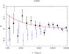 |
Fig. 1 Shear profile for the candidate SA66 (σSIS = 644 km s-1, z_spec = 0.35). The black filled squares shows the tangential component of the shear, the blue open circles the B-mode of one of the shifted profiles (for clarity). The red curve is the SIS best fit to the tangential shear. |
3.1.4. Normalization of the profiles
Before we ran the fitting procedure of the shear profiles, we had to adjust their normalization. Here we had to deal with two effects. The first one was the contamination of the sources catalogues by unlensed galaxies. Despite our selection criteria, we expected to have a significant fraction of foreground galaxies in our catalogs, thus implying a dilution of the shear signal. We also had some contamination by group members. However, because of their small number in galaxy groups and thanks to the removal of the red sequence, they did not have a significant effect on the shear measurements. We checked that, in most cases, the number density profile of the lensing sources was roughly flat in the central parts, meaning that the number of remaining group members (compared to field galaxies) in the lens catalogues was negligible. In our case, this possible contamination did not require any correction as, for instance, for rich galaxy clusters (e.g. Hoekstra 2007; Foëx et al. 2012).
The second effect was to determine the strength of the shear signal to turn the observed distortions into physical quantities. Both were treated simultaneously via the determination of the geometrical factor Dls/Ds, ratio of the angular diameter distances between the lens and the source Dls to the distance of the source Ds. We followed the same methodology as used in Limousin et al. (2009) and Foëx et al. (2012), which is based on the photometric redshifts catalogue from the T0004 release of the CFHTLS-DEEP survey. The main advantage of this catalogue is that the data were taken with the same instrument in the same photometric system as our observations. The photometric redshifts we used are in the publicly available catalogue provided by Roser Pello6, which are redshifts derived with HyperZ (Bolzonella et al. 2000) and carefully calibrated with spectroscopic samples (Ienna & Pelló 2006). Following previous works (e.g. Cypriano et al. 2004; Hoekstra 2007; Limousin et al. 2009; Oguri et al. 2009; Foëx et al. 2012), we therefore applied directly the same colour and magnitude criteria to this catalogue as were used to select the lensed galaxies in order to get a similar redshift distribution. This point required neglecting the cosmic variance, which is not always valid on the scale of 1 deg2 fields of view. We indeed checked that the redshift distribution of the D2 field (part of the COSMOS field, known to be overly dense) gives slightly different results on the average Dls/Ds than the D1, D3, and D4 distributions. In the following, we have only used the distribution of photometric redshifts from the D1 field.
Setting Dls/Ds = 0 for the galaxies with zphot < zlens, we then computed the geometrical factor (i.e. the shear strength) averaged over the full redshift distribution. In doing so, we account at the same time for the contamination by foreground galaxies in the source catalogs. We therefore simply translated the dilution of the observed shear signal by unlensed galaxies into the estimate of its strength through the distances ratio. This average geometrical factor can be inverted into an effective redshift zeff such as ⟨ Dls/Ds ⟩ = Dl,zeff/Dzeff. These effective redshifts are given in Table 2, and because of the contamination by field galaxies, they are much lower than the typical values used elsewhere to derive the strength of the shear signal of low-z clusters, i.e. zs ~ 1 (e.g. Okabe & Umetsu 2008; Radovich et al. 2008). As verified in Limousin et al. (2009), the photometric redshifts from R. Pello give consistent results compared to those obtained with the catalogue of Coupon et al. (2009).
Instead of assuming a typical source redshift, using a geometrical factor averaged over the whole redshift distribution is a better way to convert the observed shear into physical quantities. But it remains an approximation since the reduced shear is not linear in Dls/Ds (e.g. Seitz & Schneider 1997; Hoekstra et al. 2000). However, we start to fit the shear profiles at 100 kpc from the centre, which is a distance where the convergence κ is subcritical and low enough for group-scale haloes to reduce the influence of this approximation.
A last point that needed to be verified was the accuracy of the redshifts we used to estimate Dls, along with the impact on the derived lensing masses. Although we have a spectroscopic redshift for some of the SARCS objects (see Table 2), we used the photometric redshift of the central galaxy derived by Coupon et al. (2009) in most cases. First, we simply compared the spectroscopic and photometric redshifts of the 14 SARCS candidates having both values. As seen in Fig. 2, we obtained overall good agreement, with only two objects presenting a difference larger than 0.2. The first one, SA33, has its central galaxy falling in a masked region. However, the distribution of photometric redshifts (estimated with HyperZ) in the central part of the lens and corrected for the field distribution peaks at z ~ 0.65, which is a value in perfect with the spectroscopic redshift zspec = 0.64. For the second catastrophic error, SA48, a large and bright foreground galaxy ~15′′ away from the lens galaxy might contaminate its photometric redshift estimation. Given how few galaxy members there are for this lens, we could not apply the same procedure as for SA33 with a field-subtracted photometric redshift distribution. In such cases, be they a lens in a masked region, a nearby contaminating galaxy, or a close arc, estimating the redshift of the lens with only the central galaxy can be problematic.
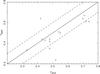 |
Fig. 2 Spectroscopic redshifts versus photometric redshifts for the SARCS objects (see Table 2). The solid line shows the equality, the two dashed lines are at ± 0.1, i.e. a typical uncertainty on photometric redshifts. |
The shear signal is fitted by γ = ⟨ Dls/Ds ⟩ × f(M), where f(M) is a function of the lens mass M. Therefore, an (over-) underestimation of the lens redshift will increase (decrease) Dls and translate into an (over-) underestimation of its mass. According to our methodology for deriving ⟨ Dls/Ds ⟩, two effects are added here when changing the redshift of the lens: the variation in the distance Dls, and the value of the contamination level, i.e. the number of galaxies in the D1 catalogue matching the selection criteria of lensed galaxies and having zphot < zlens. Since both effects have a strength that depends on the lens redshift, we tested the procedure described above in three different cases, for a low-redshift group (SA48, zspec = 0.24), one at the peak of the SARCS sample n(z) (SA50, zspec = 0.51), and one at high redshift (SA123, zphot = 1.00). For each group, we derived the average geometrical factor corresponding to different shifts in the lens redshift around its original value, and the results are presented in Fig. 3. As we can see in this plot, for a given variation Δzs, the change in ⟨ Dls/Ds ⟩ is greater for a lens with a higher redshift. However, the main variation occurs from low to medium redshifts, because the variations observed for SA50 (z = 0.51) and SA123 (z = 1.00) are very similar. For a typical zphot uncertainty of Δzs = ± 0.1, we would get an error of 20% − 30% on the geometrical factor, hence a mass over-/under-estimation of the same amount. Assuming that the zphot for most of the SARCS lenses is accurate up to this 0.1 precision, the precise knowledge of zs introduces a lower error than the statistical one (quoted in Table 2) owing to the dispersion of the galaxy intrinsic ellipticities. As detailed below, we used for the weak-lensing analysis the singular isothermal sphere mass model, which has a shear function  . In that case, a variation less than 30% in Dls/Ds induces a change less than 20% in the velocity dispersion σv. Therefore, the intrinsic ellipticity dispersion remains the principal limitation in our weak-lensing analysis. However, in specific cases with larger Δzs, we obtain a significant bias. For instance, SA48 has zphot = 0.52, and zspec = 0.24, so a geometrical factor underestimated by ~40%. Using the photometric value to fit the shear profile would have led in that case to a velocity dispersion
  , i.e. ~30% more than the value derived with the spectroscopic redshift.
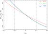 |
Fig. 3 Variation in the average geometrical factor ⟨ Dls/Ds ⟩ as a function of the shift around the true lens redshift for three groups, SA48 (red curve), SA50 (green curve), and SA123 (blue curve). The two vertical dashed lines mark the typical ± 0.1uncertainty of photometric redshifts. |
3.2. Choice of the centre
To construct a shear profile, one needs to specify its centre, which should correspond to the centre of the mass distribution. With enough constraints, its position can be considered as a free parameter of the mass model that is fitted during the weak-lensing analysis. It is also possible to use 2D pixelized mass reconstructions and to associate the highest projected density peak to the mass centre. However, since we are dealing mainly with group-scale dark matter haloes here, the shear signal is not strong enough to do that. A few attempts to fit both the mass profile and the centre (using the LENSTOOL code, Kneib et al. 1996; Jullo et al. 2007) have shown in some cases that no robust constraint can be obtained from the weak-lensing signal we have. We also tried to reconstruct 2D mass maps, but in most cases they were too noisy to derive the location of the mass centre. Moreover, Dietrich et al. (2012) have shown from a set of ground-based simulated data that, on 2D mass distributions derived from weak lensing, shifts between the real centre and the reconstructed one have a median value of 1′, therefore seriously limiting the use of this method to derive a reliable position of the mass centre.
By its definition, the SARCS sample has the advantage of giving an idea where the highest density regions are located. The SARCS lens candidates are indeed detected by a strong-lensing feature with an arc radius that corresponds to a strong-lensing event by a group-scale halo. The selection threshold of RA ≳ 2′′ limits the presence in the sample of strong-lensing events by a galaxy-scale halo enhanced by a group-scale halo, see e.g. Limousin et al. (2009). Thus we can assume that the strong-lensing system is a good indicator of the position of the actual mass centre as a high enough mass density is required, i.e. κ ≳ 1. However, we expect that this assumption might be wrong in some cases where the lens is not a regular and isolated dark matter halo but rather presents a complex morphology. For instance, Limousin et al. (2010b) showed that the SARCS lens SA66 (SL2S J08544-0121 in their paper) is a clear bimodal object spectroscopically confirmed by Muñoz et al. (2013), for which the mass centre is not associated to the centre of the strong-lensing system. As shown in Sect. 4.2, there is a non-negligible number (~15%) of such complex and multi-modal systems in the SARCS sample.
The other option usually taken when no gravitational arcs unambiguously identify the centre of the halo consists of assuming that the brightest galaxy in the dark matter halo lies in the centre of its mass distribution. The models of formation of large cD galaxies, such as infall and merging of galaxies on the central one (Ostriker & Tremaine 1975; Hausman & Ostriker 1978) or accretion of the intra cluster gas due to the cooling flow in the centre of the gravitational potential well (Cowie & Binney 1977), predict that such objects are indeed found in the centre of their host halo. This hypothesis is also supported by observational results where the cD galaxy is found in the kinematical centre (e.g. Quintana & Lawrie 1982). However, the brightest galaxy is not always a cD at rest in the gravitational potential well, but rather a large elliptical galaxy that is not necessarily located at the centre of the mass distribution. For instance, Jeltema et al. 2007 have studied a sample of seven X-ray-loud galaxy groups at intermediate redshifts (0.2 < z < 0.6), and for two of them, the brightest galaxy presents an offset ~ with the X-ray emission peak. They also found two groups where no dominant elliptical galaxy is present, but rather several ones with comparable luminosities (see also the more recent work by George et al. 2012, of the COSMOS X-ray-selected groups). In such cases, the assumption of tracing the mass centre by the position of the most luminous galaxy might be wrong as well. This problem, sometimes referred to the central galaxy paradigm (e.g. Skibba et al. 2011, for a review), is clearly a limitation to building an accurate shear profile from the position of the brightest member in a halo. In our case, it seems wiser to use the strong-lensing system to trace the position of the mass centre, and we use it for all objects in the sample, even if the lens galaxy is not the brightest one in the halo. In some cases, the strong lensing-system is indeed associated to a satellite galaxy; we discuss the impact of using the strong lensing-system as centre instead of the brightest galaxy for such groups in the Appendix.
Finally, it is worth mentioning that the mass underestimation due to small miscenterings can be limited simply by not using the central parts of the shear profiles in the fitting process (Mandelbaum et al. 2010). Because we start to fit the profiles at 100 kpc, we therefore avoid any possible underestimations in most cases.
3.3. Results
Observed shear profiles are fitted using the singular isothermal sphere model (SIS hereafter), which describes the mass density of a relaxed massive sphere characterized by a constant velocity dispersion σv. The lensing functions are written as γ(r) = κ(r) = RE/2r, where γ(r) is the shear, κ(r) the dimensionless projected mass density, and r the projected distance to the lens centre. The Einstein radius scales as  . The (one-dimensional) velocity dispersion σv is used as the free parameter to fit the SIS model and not the Einstein radius, since it requires an estimate of the source redshift. As mentioned previously, the signal-to-noise ratios that we measure are in most cases too low to get reliable information on the properties of the mass distribution, so we did not try to fit, for instance, the widely used NFW model (Navarro et al. 1997, 2004), thus avoiding poorly constrained results. We emphasize that the SIS model is only employed to derive a raw mass estimate and not to probe the shape of the mass profiles. As shown by Oguri (2006) (see also More et al. 2012), the range of image separations probed by the SARCS sample corresponds to lensing events produced by a mix of SIS (low-mass end) and NFW (high-mass end) haloes. Most of the SARCS candidates are supposed to be galaxy groups, and they present an arc radius compatible with a SIS lens. We therefore introduce a bias due to the SIS modelling in our weak-lensing analysis only for the few massive galaxy clusters in the sample. But even in these cases, given the large statistical noise we have on the lensing measurements, the SIS approximation does not result in significant variations in the total mass. An alternative would have been to stack the objects and increase the quality of the signal, as done for instance in Mandelbaum et al. (2006), Johnston et al. (2007), Leauthaud et al. (2010), Okabe et al. (2010), and Oguri et al. (2012). However, we are more interested here in the weak-lensing detection of each SARCS objects rather than a precise analysis of the mass distribution on the group scale, which could also be achieved with a combination of the weak-lensing signal on a large scale with a strong-lensing modelling of the central mass distribution and a dynamical analysis of the group members (e.g. Verdugo et al. 2011). The stacking analysis of this sample and the characterization of the mass profile will be presented in Paper II.
On the other hand, the SIS model gives results that can easily be compared to other methods to estimate the mass such as dynamical analysis (e.g. Muñoz et al. 2013). Moreover, in the case of the SARCS sample, it is straightforward to compare the weak lensing Einstein radius to the observed arc radius RA, which is equivalent to the actual Einstein radius for axisymmetric lenses. Values are given in Table 2, where the weak lensing σSIS are converted in RE(zs,σSIS) with a source redshift zs derived from the redshift distribution of More et al. (2011) with the CFHTLS T0006 release i-band limiting magnitude mlim = 24.48. For some objects, the difference between RA and RE is significant, suggesting either an inaccurate weak lensing estimation or a complicated mass distribution of the lens that affects the RA − RE relation (strong lensing associated to a satellite galaxy, large ellipticity/asymmetry of the lens, substructures, etc). A deeper study of some of these cases using strong-lensing modelling will be presented in Verdugo et al. (in prep.).
From this systematic analysis of the whole SARCS sample, we obtained constraints at the 1σ level on the SIS velocity dispersion for 89 candidates (~71% of the sample). In the rest of the paper, we call these objects weak-lensing detections. For the remaining objects, the fit of the shear profile only returns an upper limit on σv, and we will not use them in the rest of the analysis (objects labelled further as non-detected). Using a 3σ level cut to select the weak-lensing detections leads to a sample of 75 objects. However, the goal here is not to select the most secure lenses but rather to remove the most likely false detections. We checked, for instance, that some of the objects having a detection level between 1σ and 3σ present an obvious optical luminosity over-density on the luminosity map (Sect. 4.2), along with a clear strong-lensing system. That is why we chose here a rather loose selection criterion to be combined in Sect. 5.1 with the optical selection criterion. To calibrate the scaling relations in Sect. 5.3 we do, however, use only objects with a 3σ weak-lensing detection level.
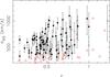 |
Fig. 4 Velocity dispersion derived from the fit of the shear profile using the SIS model. Red open triangles show the upper limit on σv for those objects not having a 1σ weak-lensing detection. Open circles are candidates with a weak-lensing detection less than 3σ, filled circles are those having a reliable detection (above 3σ). |
The distribution of the SARCS candidates in the z − σv plane is shown in Fig. 4. The average velocity dispersion of the 89 weak-lensing detections is ⟨ σv ⟩ = 618 ± 197 km s-1, corresponding to a rich group or a poor cluster, depending on where the boundary between the two regimes is drawn. From Fig. 4, we see that the distribution σv(z) is fairly homogeneous over the redshift range. We detect, however, more massive objects above z = 0.5. From a weak-lensing analysis it is expected because for a source at a given redshift, the lensing strength decreases for lenses at higher redshifts. Therefore it is normal to observe a higher fraction of more massive systems at higher redshifts. We also see in Fig. 4 that these high-redshift objects present larger error bars on the velocity dispersion, owing to the lower density of available background galaxies to measure the shear signal. It is interesting to notice that we do not observe a strong trend between the non-detected objects and their redshift. This lack of correlation suggests that the intrinsic quality of the ground-based optical images (seeing, pixel size) that we used is the main limitation to detecting low-mass objects, rather than the noise induced by lower densities of background galaxies.
Finally, it is worth mentioning that at the low-mass end of the sample, the shear signal is weak enough to be close to the noise level. As a result, our weak-lensing measurements for such objects have to be taken with caution. We emphasize here that we are more interested in detecting of the objects rather than in getting accurate mass estimates. On the group scale, we probably lose some real lenses and also have some false detections or galaxy-scale systems among our 89 objects. The cross-checking with the optical properties (Sect. 5.1) shows, for instance, that some of the weak-lensing detections have no optical counterpart, corresponding to those cases where our lensing procedure fits noise.
Looking in more detail at the properties of these non-detections, it appears first of all that they mainly correspond to SARCS candidates with a small arc radius. We indeed have 29 objects with RA < 4′′, i.e. ~78% of the non-detections. The whole SARC sample contains 88 objects with RA < 4′′ (~70% of the sample), a slightly lower value that simply reflects that less massive objects (i.e. with smaller arc radius) are more difficult to detect via weak lensing. We only have two candidates not detected in weak lensing with RA > 5′′, one of them having a large arc radius, SA104 with RA = 11.7′′ (zphot = 0.15). This object (rank 2 in More et al. 2012) shows a single very large elliptical galaxy without any obvious companion around. Given the arc radius of ~12′′, this object should have much more members because it would correspond to a poor cluster. We then can safely consider this object as a false detection in the SARCS sample. The other object is SA41 (RA = 6.1′′, zphot = 0.52). This object presents a bimodal light distribution. A wrong choice of the centre to compute the shear profile could be the reason for the weak-lensing non-detection. However, using a different centre does not improve the constraints (see Appendix).
Among the 37 non-detections, we have 25 candidates with a rank less than 3, i.e. ~68%. This value is slightly higher than the ratio obtained for the entire sample, which contains ~57% of such low-ranked candidates. It suggests that the threshold rank ≥ 2 used to build the initial SARCS sample is not strong enough to prevent keeping false detections. In Sect. 5.1, we discuss the properties of the most secure candidates in terms of the initial selection parameters (rank and arc radius).
Besides those systems falsely identified as strong lenses, one can think of several hypotheses to explain why objects with a small arc radius are not detected with the weak lensing method. First, these strong lensing features are most likely produced by less massive systems (or even galaxy-scale haloes), which do not produce a weak-lensing signal strong enough to be detected with ground-based data. Second, a star field that is too sparse to properly sample the PSF across the field-of-view can reduce the quality of the galaxy shape estimation, hence introducing more noise into the signal. On the other hand, a field with too many large diffracted stars has a smaller effective area to measure the shear signal, which can bias the weak-lensing analysis. Third, the intrinsic mass distribution of the lens might as well be a strong factor of noise in the measured shear signal. We indeed use the simplest weak-lensing analysis that assumes circular symmetry. In the case of highly elliptical mass distributions, such an approximation can result in a significant underestimation of the shear. It can also generate apparent small arc radius, which are not representative of the total mass of the halo, thus explaining why we have weak-lensing detections for some candidates with small RA. For multi-modal systems, the question of the centre and the fit to a single halo might also bias the mass determination. In the Appendix, we present some results for such complex systems, along with some cases where the strong-lensing system is not associated to the brightest galaxy in the halo but to a satellite galaxy. We emphasize here all these possible reasons just to recall that a weak-lensing detection is sufficient but not necessary to conclude that we are observing a massive halo.
3.4. Comparison with previous mass measurements
Several SARCS groups have been already analysed using different data sets and methodologies:
-
Weak lensing: with the CFHTLS T0004 release, Limousinet al. (2009) derived weak lensingconstraints on σSIS only for five groups of their sample of 12 ob-jects. With these five objects, we find an average ratio ⟨ σWL/σSIS ⟩ = 0.93 ± 0.10 (where σSISare the velocity dispersions derived in this work and σWL thosefrom Limousin et al. 2009).There is only one group in the sample of Limousinet al. (2009) for whichwe did not get a weak-lensing detection, SA122 (zphot = 0.69, RA = 2.8,rank = 3.0) and for which Limousinet al. (2009) only obtained an upperlimit on σSIS.
-
Strong lensing: eight objects were analysed by Limousin et al. (2009) using the CFHTLS ground-based images, and four new groups have been studied with HST data (Verdugo et al., in prep.). To compare the results of Limousin et al. (2009) to ours, we have converted their Einstein radius into σSL assuming the source redshift given in Table 2. With these 8 + 4 groups, we obtain an average ratio ⟨ σSL/σSIS ⟩ = 0.92 ± 0.25.
-
Dynamical analysis: seven objects have been studied by Muñoz et al. (2013) using VLT/FORS2 spectra. Here we obtain an average ratio of ⟨ σdyn./σSIS ⟩ = 0.61 ± 0.25.
Even though our weak lensing methodology follows that of Limousin et al. (2009) closely (same procedure for selecting the lensed galaxies and estimating their shape parameters, same normalization of the shear profiles), we managed to measure σSIS for 11 of their sample of 12 groups, while they obtained constraints only for five of them. We attribute this increased number of detection to our statistical analysis of the shear signal. On the other hand, the results we have are very similar with a ratio of ~0.9 and a small scatter of 10%. Our velocity dispersions are also compatible on average with the values derived from the strong-lensing analysis of Limousin et al. (2009) and Verdugo et al. (in prep.), again with a ratio of ~0.9, but with a larger scatter of ~25%. This seems to indicate that these groups do not present very high ellipticity with a major axis aligned along the line-of-sight or, equivalently, a high concentration that could artificially enhance the measured mass when extrapolating the strong-lensing constraints to the larger scales probed with weak-lensing signal.
The comparison of our measurement with the dynamical velocity dispersions derived by Muñoz et al. (2013) is more puzzling. We obtain indeed a ratio of ~0.6 with a scatter of ~25%. Among the seven groups, six have a dynamical velocity dispersion that is smaller than the weak lensing one. Only one group, SA72, has σdyn > σWL, with compatible values at the 1σ level given the high uncertainty on σdyn. Muñoz et al. (2013) argue that one reason of such a discrepancy could arise from the choice of the SIS model to characterize the actual mass distribution of the groups. With numerical simulations, they also show that mass estimates derived from the velocity dispersion of galaxies in a halo can be underestimated up to 20%. This is, however, not enough to explain the discrepancies observed here. Another possibility to account for the differences between the lensing and dynamical results would be the presence of massive structures along the line of sight. Because the weak-lensing signal is produced by all the projected matter between the lensed galaxies and the observer, groups and clusters of galaxies or even large-scale structures can affect the shear signal and induce and overestimation of the mass. Using the Millennium simulation, Hoekstra et al. (2011) find that randomly positioned massive structures do not statistically bias the weak-lensing mass estimate of a galaxy cluster but instead increase its uncertainty, with values comparable to those owing to the intrinsic dispersion of the galaxies ellipticity. Most of the overestimated masses they obtained have an excess less than 20%, but going up to a factor ~2 for some objects. Such projection effects could therefore explain the higher weak-lensing masses we have. We can also invoke a poor lensing signal-to-noise ratio from which the weak-lensing analysis can return biased masses. Because the objects analysed by Muñoz et al. (2013) are mostly low-mass groups with σdyn < 500 km s-1, they indeed do not produce a strong shear signal, possibly leading to wrong estimates. However, we observe a similar discrepancy for all objects, which suggests that this systematic difference in the velocity dispersions is due to the methodologies employed, rather than to the groups properties or poor constraints. In fact, the estimation of galaxy groups and clusters’ velocity dispersion is known to be biased low by several effects (see e.g. Biviano et al. 2006, and references therein), such as the inclusion of interlopers (i.e. infalling galaxies along filaments), the rejection of high-velocity galaxy members, presence of substructures, or the so-called velocity-bias (i.e. different velocity dispersions between galaxies and the dark matter). We are currently increasing the number of groups analysed via the dynamical methodology, and we will explore the discrepancy between the lensing and dynamical estimate of the groups velocity dispersion in more detail (Motta et al., in prep.).
4. Optical properties
Although the weak-lensing results suggest that some of the SARCS candidates are galaxy-scale lenses or false detections, we did the optical analysis for all objects in the sample. We therefore intend to make a cross-correlation of the two analyses to derive a sample of the most bona fide SARCS groups candidates used to constrain the optical scaling relations.
4.1. Richness and optical luminosity
We derived the optical properties of the SARCS lens candidates from the bright galaxies that belong to the red sequence. Because most of the SARCS objects are groups with few galaxies, we did not attempt to fit this red sequence as usually done when dealing with rich galaxy clusters. We used the same criteria for all the candidates and defined the red sequence as the region in the colour-magnitude diagram where galaxies have a r′ − i′ colour close to that of the lens galaxy, i.e. the one at the centre of the strong-lensing system. In the cases where this lens galaxy is not the brightest one but rather a satellite galaxy, we used the colour of the former to define the red sequence. To account for the expected slope of the red sequence (e.g. Stott et al. 2009), we chose asymmetric limits and selected galaxies with (r′ − i′)lens − 0.2 < r′ − i′ < (r′ − i′)lens + 0.15. As said previously, the galaxy at the centre of the strong-lensing system is not necessarily the brightest one, so its colour (r′ − i′)lens can be slightly different from that of the brightest member, which is usually taken as reference; however, it gives a robust estimator of the group members colour, since by definition, it belongs to the group. Because the colours are derived from magnitudes estimated in a fixed aperture of 3′′, this (r′ − i′)lens colour tends to be underestimated for systems presenting an arc radius RA ≤ 3′′ where the lens galaxy is close to the strong lensing feature (a blue arc in most cases). For these objects, we used the average colour of the surrounding bright galaxies that are most likely part of the system.
We restricted the red sequence to an absolute magnitude Mi′ = −21. In doing so, we roughly probed a constant fraction of the luminosity function, which allows direct comparison from group to group regardless of their redshift. Focussing on the brightest galaxies also avoids the fall out of the completeness magnitude of the CFHTLS observations for groups at high redshifts.
In Limousin et al. (2009), the group members were visually selected and no background correction was applied. Here, since we adopt an automated approach for all objects, we also have to account for the contamination by field galaxies. We determined the density of galaxies falling in the definition of the red sequence of each group in a reference field. To keep it simple, we used the 1 deg2 image of the field where the group was found (for systems in the WIDE part of the CFHTLS survey, we only used the central pointing as reference). To get a rough estimate of the fluctuations due to local over-/under-densities in the distribution of field galaxies, we computed the background density in 1000 circular patches randomly positioned in the reference field. The size of these patches is chosen to match the area where group members are counted, i.e. within a projected radius of 0.5 and 1 Mpc from the central galaxy. We chose to compute the optical properties within two different radius in order to test its influence on the calibration of the scaling relations.
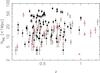 |
Fig. 5 Richnesses estimated within 1 Mpc using the bright red galaxies of the 126 SARCS candidates. Open red triangles are objects without a 1σ weak-lensing detection, open circles have a detection between 1 and 3σ, filled circles are those with a detection above 3σ. |
To reduce the impact of overestimating the local density of field galaxies, which can lead to a negative number of galaxies for poor groups (as well as for systems falsely identified as a group), we divided the area where galaxies are counted into concentric annuli. The background subtraction was done in each of these annuli, and we finally took the sum of only the positive counts excesses. The richnesses we derived (i.e. the number of galaxies within our selection criteria) are the average of these sums over the 1000 values of the background densities. The scatter around this average gives a rough estimate of the corresponding statistical error. We did the same to compute the optical luminosities accounting for both the k-correction and the passive evolution of an elliptical galaxy (values derived from the synthetic SED model of Bruzual & Charlot 2003). For consistency, we applied this method to all the SARCS candidates, regardless of whether they are false detections, poor groups, or poor clusters for which a usual background subtraction works fine. The distribution of richnesses and optical luminosities for the SARCS objects are given in Figs. 5 and 6. Within an aperture of 1 Mpc around the centre of the strong-lensing system and cutting the luminosity function at Mi′ = −21, the sample covers richnesses up to 70 galaxies and luminosities up to ~6 × 10¹² L⊙. Both distributions are roughly homogeneous in redshift, and are dominated by group-scale objects with N ~ 5−20 and L ~ 0.5−1.5 × 10¹² L⊙.
We chose to derive the optical properties of the SARCS candidates from the galaxies within their red sequence. These galaxies are indeed easier to detect and select (stronger contrast with the population of field galaxies), and most of studies about the optical scaling relations make use of this specific population of early-type galaxies. However, we would like to emphasize here that such a selection can introduce some systematics into the analysis. It has indeed been observed that at higher redshifts, groups and clusters contain a greater portion of blue star-forming late-type galaxies (Butcher & Oemler 1984; Ellingson et al. 2001; Lubin et al. 2002), with, on the other hand, a smaller fraction of red passive early-type galaxies (Smail et al. 1998; Kodama et al. 2004; De Lucia et al. 2007). This evolution of the red sequence, where the blue spirals evolve into red elliptical galaxies with a transient state of green galaxies (Balogh et al. 2011b), naturally introduces a bias into our galaxy selection as a function redshift since we used a fixed broad red sequence for all objects. Another possible source of systematics in the estimation of richnesses and optical luminosities is the actual fraction of the galaxy population that inhabit the red sequence. For instance, Zabludoff & Mulchaey (1998) have studied a sample of 12 nearby poor galaxy groups and found significant variations (up to a factor 2) in the fraction of early-type galaxies. Similar variations in the galaxy population from group to group have been obtained by Jeltema et al. (2007) at intermediate redshifts. Therefore, we do not probe the same fraction of group members for each object in our sample. However, given the relatively large size of the SARCS sample and its broad redshift range, we expect to average such effects (intrinsic variations and redshift evolution), so we did not attempt to correct them or to include the green and blue galaxies in the analysis.
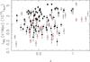 |
Fig. 6 Same as Fig. 5 for the optical i′-band luminosities estimated within 1 Mpc using the bright red galaxies of the 126 SARCS candidates. |
4.2. Morphological classification
From the catalogues of galaxies falling in the red sequence (to get more galaxies and less statistical noise when drawing the luminosity contours, we pushed the limiting magnitude to Mi′ = −20 instead of −21), we computed luminosity maps following Limousin et al. (2009). The 15′ × 15′ field-of-view around the lens is divided into cells of 20 × 20 pixels. From the centre of each of these cells (the pixels of the luminosity maps), we looked for the five nearest galaxies belonging to the red sequence, a low enough value to avoid oversampling. The luminosity density of the corresponding pixel is simply the sum of the luminosity of these five galaxies divided by the circular surface covered by the farthest one. The maps of the luminosity density are then smoothed by a Gaussian kernel with an FWHM of seven pixels (~25′′). We checked that the shape of the resulting maps are weakly dependent on the pixel size or the smoothing width.
As stated previously, we did not clean the catalogues of the red galaxy members from field galaxies. The maps therefore suffer from the background contamination, but we can assume it to be roughly homogenous across the field, thus not leading to strong shape distortions of the group/cluster itself. However, this can be wrong for groups with low numbers of galaxies in the red sequence. Despite our adaptive smoothing, the classification between a regular or elongated object can indeed be affected by statistical noise due to local variations in the density of field galaxies. On the other hand, because of the large width of the red sequence we used, we expect to pick up over-densities of galaxies that are not necessarily linked to the initial target (i.e. not a multi-modal object). In fact, this can be used as a tool to trace the cosmic web and reveal large-scale structures around galaxy groups (Cabanac et al., in prep.).
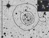 |
Fig. 7 Luminosity density contours (in black) for SA15 equal to 106, 4 × 10⁶, 7 × 10⁶, 107, and 1.3 × 10⁷ L⊙ kpc-2. The white cross marks the galaxy at the centre of the strong-lensing system. The black vertical line on the left is 1 Mpc long. SA15 is at z = 0.44. The stamp in the top-right corner shows a 30′′ × 30′′ colour image of the system. |
Once the maps were built, we visually inspected them to assess the luminous morphology of the SARCS objects according to the shape of the luminosity contours, whose levels were adapted for each object. However, we checked that the value chosen for the innermost luminosity contour does not influence the occurrence of high-luminosity peaks, i.e. the multi-modal groups definition. We sorted the groups according to their morphology in four classes:
-
false detection or galaxy-scale strong lensing feature (i.e. no clearover-density in the map) → 30 objects;
-
regular (i.e. roughly circular isophotes around the strong-lensing system) → 39 objects;
-
elongated (i.e. elliptical isophotes with a roughly constant position angle form inner to outer parts) → 40 objects;
-
multi-modal (i.e. 2 or more peaks in the central part of the map) → 17 objects.
Figures 7–9 present the luminosity map for a regular group (SA15), an elongated group (SA2), and a bimodal group (SA90). Multimodal class refers here only to two or more peaks in the luminosity map found within a 0.5 Mpc radius of the strong-lensing system. Extending this limit to a larger radius would increase the number of objects in this class, e.g. 23 members if we look up to 1 Mpc from the centre. However, in these cases we are most likely observing two distinct objects (or an ongoing merging event) rather than a single halo since, given the mass range of these groups, the virial radius is expected to be ≲1 Mpc (see e.g. Muñoz et al. 2013). We look for a trend between the morphological class and the redshift or mass of the objects in Sect. 5.1, after defining the final sample of the best candidates.
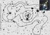 |
Fig. 8 Luminosity density contours (in black) for SA2 equal to 2 × 10⁶, 4 × 10⁶, 7 × 10⁶, 1.5 × 10⁷, and 2 × 10⁷ L⊙ kpc-2. The white cross marks the galaxy at the centre of the strong-lensing system. The black vertical line on the left is 1 Mpc long. SA2 is at z = 0.48. The stamp in the top-right corner shows a 30′′ × 30′′ colour image of the system. |
From this qualitative morphological classification, it appears that the main part of the SARCS candidates are groups or poor clusters with irregular shapes, either elongated or more complex, i.e. (40 + 17)/96 ~ 60% of the optically detected lenses. This suggests that groups of galaxies are mostly in a young dynamical state. In the context of the large-scale structure formation and evolution, this is somehow expected since groups are continuously forming and merging into more massive clusters (e.g. Evrard 1990; Bekki 1999). Paper II will present a more quantitative analysis of the groups morphology, along with studying correlations to the groups’ environment.
5. Combining the weak lensing and optical analyses
5.1. Selection of the most secure candidates
As mentioned in Sect. 2.2, the thresholds applied to the arcfinder algorithm were chosen to favour completeness over purity. Despite the visual ranking performed by three different persons, the final SARCS sample still contains galaxy-scale lenses and even some false detections. Both the weak-lensing and the optical analyses have indeed shown that some objects do not reach our criteria for selection as a group-scale lens.
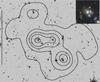 |
Fig. 9 Luminosity density contours (in black) for SA90 equal to 1.5 × 10⁶, 4 × 10⁶, 7 × 10⁶, 107, and 1.5 × 10⁷ L⊙ kpc-2. The white cross marks the galaxy at the centre of the strong-lensing system. The black vertical line on the left is 1 Mpc long. SA90 is at z = 0.53. The stamp in the top-right corner shows a 30′′ × 30′′ colour image of the system. |
From the weak-lensing analysis, we end up with a reduced sample of 89 objects with a weak-lensing detection. The rejected objects are either false detections, not massive enough haloes (very poor groups or galaxy-scale lenses) or objects with shear signal that is too noisy to derive a secure SIS velocity dispersion (sparse data, morphology too complex for a simple spherical mass model, etc.). As said in Sect. 3.3, they present more low-ranked objects with smaller arc radius RA than in the total sample.
From visual inspection of the colour images and the luminosity maps, the initial SARCS sample got reduced to 96 objects among which 39 present regular isophotes, 40 elongated ones, and 17 have a multi-modal configuration. Here, we rejected all the candidates for which we do not observe a clear over-density of light associated to the strong-lensing system, i.e. objects where the lensing feature is in a poor environment without evidence of a population of galaxies with similar colours. As for the weak lensing selection, this optical selection mainly rejects SARCS candidates with a small arc radius, i.e. probably galaxy-scale objects or very poor group lenses. Only four rejections are associated to arc radius RA > 3′′ and most likely correspond to false detections, e.g. edge-on spiral galaxies.
While the optical selection removes 30 objects, the weak lensing selection rejects 37 candidates, so a similar number of possible lenses. Interestingly, the two methods have 21 rejected candidates in common, which are most certainly not group-scale lenses and can be securely removed from the final sample. On the other hand, we have 16 candidates not detected in weak lensing but flagged as probable groups from their luminosity maps. Among them, only four objects have regular isophotes, which suggests that we do not measure a good enough shear signal because of the complex morphology of the mass distribution (multi-modal or highly elliptical). We also have nine objects for which we managed to put constraints on σSIS, but which do not have an obvious optical counterpart (our richness estimator gives for all of them a null or negative value). We visually inspected these dark lenses, and for four of them we found a significant galaxy concentration less than 5’ away from the supposed strong-lensing system. In these cases, the shear signal that we measured is most likely due to a close (in projection) massive structure not associated to the SARCS candidate. In two other cases, the PSF map derived from the field of stars shown an irnegular pattern that might generate a false shear signal. For the three remaining objects, we could not find any obvious explanation for the measured shear signal given that the optical images clearly show the absence of a galaxy concentrations around the SARCS candidate.
Finally, the combination of our selection criteria leads to a sample of 80 lenses ranging from group- to cluster-scale haloes. Their weak-lensing and optical properties are given in Table 2. In terms of the morphological distribution of this sample of most secure lenses, we have 34 objects with regular isophotes (~42%), 33 with elongated/elliptical ones (~42%), and 13 multi-modal groups (~16%) with a second luminosity peak closer than 0.5 Mpc to the strong-lensing system. The different ratios are roughly similar to those obtained for the 96 candidates having a clear optical detection, and our final sample still contains a large proportion of objects with an irregular light distribution (~57%). The average velocity dispersions in each morphological class are all compatible within their 1σ statistical scatter since we obtain 592 ± 175 km s-1 for the regular groups, 589 ± 201 km s-1 for the elongated ones, and 716 ± 147 km s-1 for the multi-modal, i.e. a slightly higher value. We also looked for any redshift trend, but the three classes have a very similar average redshift.
The initial sample has ~70% of objects with RA < 4′′ (observed RA, not derived from σSIS) and ~57% objects ranked less than 3, which is the threshold used in More et al. (2012) to define the most promising candidates. In our final sample we obtain percentages of ~63% and ~49%: our optical and lensing criteria result in a sample with a higher proportion of promising candidates (based only on the visual inspection of the strong lensing features) and with larger arc radius. If we assume that the best group- and cluster-scale lens candidates can be defined a priori as those having both a rank ≥3 and RA ≥ 4′′, then our final sample contains 18/20 of the best candidates in the initial SARCS sample, which suggests that these two criteria are fairly robust to be able selecting such real lenses on the group scale.
To reduce the impact of unreliable measurements, we only keep the objects with a 3σ weak-lensing detection to fit the scaling relation. This subsample of the most secure candidates according to our combined weak-lensing and optical analysis contains 67 objects. In doing so, we lose some objects at high redshifts, without improving the dispersion in richness or optical luminosity (see Figs. 4–6). Because we have 14 objects (13 with an optical confirmation, among which 2 have a spectroscopic confirmation and a strong lensing model) with a weak-lensing detection level between 1 and 3σ, we lose ~16% of the 80 lenses’ subsample defined here. Therefore, this sample with a larger statistic, especially at high redshift, will be used in other works to study the population of galaxy groups (e.g. Verdugo et al., in prep.).
 |
Fig. 10 Velocity dispersion derived from weak lensing as a function of optical richness (first row) and luminosity (second row) estimated with the bright red galaxies in 2 apertures, 0.5 Mpc (left column) and 1 Mpc (right column). We used only the sample of the 80 candidates defined in Sect. 5.1 (error bars on each individual measurement are omitted for clarity, see Table 2). Green points with error bars highlight the increase in σv with richness and luminosity after binning the SARCS lenses according to their observed richness or luminosity. |
5.2. Scaling relations on the group scale
We used the sample of the 80 most secure candidates as defined previously to look for correlations between the mass derived from weak lensing and the optical properties. Such scaling relations, characterized by power laws, have been observed on different mass scales and redshifts (e.g. Lin et al. 2003, 2004; Popesso et al. 2005; Brough et al. 2006; Becker et al. 2007; Johnston et al. 2007; Popesso et al. 2007; Reyes et al. 2008; Mandelbaum et al. 2008; Rozo et al. 2009; Andreon & Hurn 2010; Foëx et al. 2012). Usually, scaling relations are investigated using spherical NFW mass at a given density contrast, e.g. M200, since they are related to the total virial mass. Because the SARCS sample is mainly made up of galaxy groups, we kept our weak-lensing analysis to its simplest version with only estimates of the SIS velocity dispersion. As the SIS model is already a significant approximation of the actual mass distribution, we did not use SIS masses in a given aperture because it would increase the scatter of the correlations, but simply used the SIS velocity dispersions. Moreover, the lack of information on the actual mass profile of the lenses means we do not have estimates of their virial radius, although Muñoz et al. (2013) give a raw estimation for some of the groups. Therefore, we used richnesses and luminosities derived in fixed physical apertures (0.5 and 1 Mpc) regardless of the mass and the redshift of the objects.
Our results are presented in Fig. 10. In all cases, we observe quite a large dispersion in σSIS with scatters ranging from 15% to 35%, without any obvious trend as a function of richness or luminosity. However, when the objects are binned according to their richness or luminosity, we detect the expected correlations, where the more massive objects are more luminous and have more galaxies populating their red sequence.
It is interesting to note in both right-hand panels of Fig. 10 the presence of a clear outlier in the bottom right-hand corner. This object is embedded in a large-scale structure that extends over several Mpc. It is located close to the node of this filamentary structure, so when counting galaxies up to 1 Mpc, we face contamination by the surrounding clumps of galaxies. We also observe three outliers for the N − σv relations with an apparently over-estimated velocity dispersion given the richness (σv > 800 km s-1, N0.5 Mpc < 10). However, these objects do not appear as outliers in the L − σv relations. In two cases, the presence of two bright galaxies of similar magnitude in the centre can explain this behaviour (for the third one, another bright galaxy with similar colours falls into the 0.5 Mpc region from the lens). However, owing to the large size of the red sequence, we cannot securely distinguish between group members and field galaxies from which projections effects could explain the observed high luminosity given the richness of these three objects. Projection effects could also be responsible here for over-estimated lensing masses.
A more accurate calibration of these relations will be presented in Paper II, where groups will be stacked and outliers removed, such as objects in large-scale structures or with a very disturbed light morphology.
5.3. From poor groups to rich clusters
To get a wider range in mass, we combined this sample of the best SARCS candidates with the sample of rich and massive galaxy clusters presented in Foëx et al. (2012). These 11 clusters are part of the EXCPRES sample (Evolution of X-ray galaxy Cluster Properties in a REpresentative Sample, Arnaud et al. in prep.), which was designed as the REXCESS sample (Böhringer et al. 2007) in order to study the evolution of the X-ray properties of clusters. The full EXCPRES sample contains 20 clusters in the redshift range 0.4 < z < 0.6, observed with XMM-Newton. Only clusters with an X-ray luminosity LX > 5 × 1044 erg/s in the [0.5–2.0] keV band within the detection radius were selected for an optical follow-up at the CFHT. The X-ray properties and the results of the weak-lensing analysis of this subsample of 11 clusters are presented in Foëx et al. (2012).
To be consistent with the work on the SARCS sample, we analysed the optical images (Megacam data) of the EXCPRES clusters with the exact same procedure as used here to get the richnesses and luminosities. In total, we have 67+11 objects to adjust four scaling relations, σSIS − N0.5 Mpc, σSIS − N1 Mpc, σSIS − L0.5 Mpc, and σSIS − L1 Mpc. We used single measurements to fit the correlations, not binned values as in other works, such as Reyes et al. (2008) and Leauthaud et al. (2010). Some of the SARCS candidates are located close to the edge of the MegaCam field-of-view, at a projected distance smaller than the size of the aperture used to derive the optical properties. We removed these objects from the fit of the scaling laws, one for the correlation at 0.5 Mpc and four for those at 1 Mpc (objects notified by an asterisk in Table 2).
To get more quantitative results, we fitted the correlations using the bootstrapping orthogonal BCES estimator (Bivariate Correlated Errors and intrinsic Scatter, Akritas & Bershady 1996) as done in some previous works, e.g. Morandi et al. (2007), Pratt et al. (2009), Foëx et al. (2012). The main advantage of this approach over simple linear regression is that it accounts for the intrinsic dispersion of the objects around the best fit. This dispersion needs to be included and evaluated in the fit. It indeed gives a crude idea of the impact of some physical processes that cause a departure from the theoretical predictions. For instance, the large intrinsic dispersion observed in the mass-X-ray luminosity scaling relation is a good tracer of the physics that take place in clusters of galaxies such as radiative cooling, pre-heating, or feedback from supernovae (e.g. Voit 2005 for a review).
To optimize the fit of the scaling relation and reduce the correlation between its logarithmic slope and normalization, we normalized both variables by a pivot representative of the sample: 10 and 20 for richnesses in 0.5 Mpc and 1 Mpc, 1012 L⊙ and 2 × 10¹² L⊙ for luminosities. The velocity dispersions are normalized by 600 km s-1. The results of the BCES estimator are given in Table 1 and Fig. 11 shows the best BCES fit for the σSIS − N1 Mpc scaling law. As in Lin et al. (2004) and Foëx et al. (2012), we also give the value of the Spearman correlation coefficient ρ, which shows the degree of monotony of a given correlation.
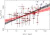 |
Fig. 11 Richness-velocity dispersion scaling relation. The black solid line shows the best BCES orthogonal fit of the N1 Mpc − σSIS relation using the SARCS most secure candidates (red points) and adding the EXCPRES galaxy clusters of Foëx et al. (2012) (blue open triangles). The grey shaded area gives the statistical 1σ uncertainty given by the best fit parameters (statistical dispersion σstat). The red line (and corresponding shaded area) is the best fit using only the SARCS most secure candidates. |
Summary of the fitting results for the scaling relations (σ/σ0) = A × (Obs./PObs.)α.
First of all, the correlations appear to be roughly the same when working at 0.5 or 1 Mpc from the centre. This basically means that the choice of the aperture in which richnesses and luminosities are estimated is not a dominant parameter. This has already been observed in similar studies (e.g. Andreon & Hurn 2010; Foëx et al. 2012) with consistent results using either a fixed aperture or scaling it with mass. Thanks to the large number of objects, we obtain small statistical dispersions, the intrinsic scatter around the best fit being the main source of noise (see Fig. 11) and 12, with σint ~ 0.11 (dex). The correlations are fairly strong with Spearman coefficients of ρ ~ 0.6−0.7: both the richness and the optical luminosity of the bright red galaxies in a halo are good tracers of mass. We can assess the quality of our best fits as mass proxies simply by converting richnesses and luminosities into σv,proxy and looking at that average relative error over the sample R = ⟨ | (σv,WL − σv,proxy)/σv,WL | ⟩ (see Table 1). According to this criterion, our scaling relations are efficient for recovering velocity dispersions with an accuracy of better than ~25%.
While the hierarchical model of structure formation predicts a number of subhaloes proportional to the mass of the parent halo, i.e. N ∝ M (e.g. De Lucia et al. 2004; Gao et al. 2004), including baryons in numerical simulations results in a decrease in the number of galaxies for a halo of higher masses, i.e. N ∝ Mα with α < 1 (see e.g. White et al. 2001; Berlind et al. 2003). Several mechanisms can be responsible of this reduced slope, such as a decrease in gas cooling and star formation efficiency (Springel & Hernquist 2003; Borgani et al. 2004; Kravtsov et al. 2004) or an increased merger/destruction rate of galaxies in higher mass objects (White et al. 2001; Lin et al. 2003). Our results for the σv − N relations are in good agreement with theoretical predictions from numerical simulations with a slope of 0.33 (e.g. Evrard et al. 2008; Lau et al. 2010), as well as similar work (Andreon & Hurn 2010). However, we do not observe any significant evidence of the influence of physical processes that might affect the galaxy population. For the σSIS − L relations, we obtain slightly steeper slopes than the σSIS − N correlation with values that are not consistent with a constant mass-to-light ratio. This result suggests that the physical mechanisms inside a dark matter halo are more efficient to affect the luminosity rather than the number of red-sequence galaxies, including for instance ram pressure stripping or galaxy harassment (see e.g. Treu et al. 2003; Poggianti 2004; Boselli & Gavazzi 2006). The presence of a higher fraction of galaxies with evolved stellar populations in higher mass objects has also been invoked to explain the increase in the mass-to-light ratio with mass (e.g. Bahcall & Comerford 2002). However, this assumption has been ruled out by Popesso et al. (2007) and their study of the fundamental plane of the cluster ellipticals, showing that they have a constant mass-to-light ratio that cannot explain the variations in the total mass-to-light ratio of clusters. We intend to use our spectroscopic surveys of the SARCS groups to investigate this hypothesis in more detail and down to lower-mass objects in Paper II.
We also fit these scaling relations using only the sample of galaxy groups. We obtained slopes that are slightly lower but consistent within 2σ uncertainties with the groups+clusters combined fits (see Table 1; also see Figs. 11 and 12). This result is not surprising since we use bootstrapping to derive the best fit parameters, which gives more weight to the SARCS groups as they are more numerous than the EXCPRES clusters. With the relations calibrated with the SARCS objects alone, we derived the associated R value. The σSIS − L1 Mpc scaling gives R = 24% (22% when applied on the SARCS sample only, 37% for the EXCPRES clusters alone), and the σSIS − N1 Mpc relation gives R = 25% (23% and 34%). These relations give similar accuracies despite lower slopes. This is mainly the result of the different sizes of the two samples, the SARCS one dominating the statistic. We find higher R values for only the EXCPRES sample, suggesting a break in the scalings between the low- and high-mass ends of the combined sample. However, since we do not obtain statistically significant differences in the slopes of the scaling relations between groups and groups+clusters (discrepancies lower than 3σ), we cannot reliably distinguish between a single population of similar objects over the whole mass range and the presence of two distinct subpopulations.
5.4. Comparison with previous works
Although this work is the first one based on such a large sample of strong lensing groups, we are not the first to investigate the group properties through some scaling relations. As stated previously, groups have already been extensively studied with different baryonic tracers, from X-ray or optical observations. Despite some difficulty making proper comparisons (e.g. different ways of defining the optical richness, measure the X-ray luminosity, etc), we review here some of these works.
From the X-ray point of view, Jeltema et al. (2006, 2007) present the analysis of a sample of nine X-ray emitting galaxy groups at intermediate redshifts (Mulchaey et al. 2006). In particular they find that these intermediate-redshift groups present similar properties as local groups, thus excluding strong non-standard redshift evolution. The X-ray properties of these objects (temperature, luminosity, entropy) follow the scaling relations obtained with galaxy clusters and/or nearby galaxy groups (see also Mulchaey & Zabludoff 1998). In Sect. 5.1, we showed that we obtained large scatters in the velocity dispersion at a given richness or optical luminosity, which was also observed by Jeltema et al. (2006) for a given temperature or X-ray luminosity of the gas.
More recently, a large sample of 200 X-ray galaxy groups up to a redshift of 1 has been drawn from the COSMOS field (Scoville et al. 2007) and studied with a weak-lensing analysis to put constraints on the mass-X-ray luminosity scaling relation by Leauthaud et al. (2010). They find very good agreement with other studies, i.e. that this correlation can be characterized by a single power law over a very wide range in mass (see also Foëx et al. 2012). Despite some hints of a possible break of similarity on the cluster scale, we have shown in the previous section that a single power law also gives an acceptable fit of the scaling with richness and luminosity from poor groups to rich clusters. They claim to observe little evidence for a non-standard redshift evolution of the relation, but without a strong statistical significance. Their work therefore also confirms that galaxy groups are following the same scalings as galaxy clusters rather than presenting special properties. Giodini et al. (2009) studied some galaxy groups and poor clusters observed in the COSMOS field. Their analysis of the stellar mass fraction associated to the galaxy members again showed no evidence of a non-standard redshift evolution since their scaling relation agrees with the one obtained for local clusters (see also the work by Connelly et al. 2012). Their results on galaxy groups are also in good agreement with those for only galaxy clusters, again supporting the idea that galaxy groups are not a particular population of haloes but just a scaled-down version of clusters, as expected in the simple model of hierarchical structure formation and evolution.
As stated in Sect. 3.2, using the same COSMOS data, George et al. (2012) confirmed the findings of Jeltema et al. (2007) about the BGG/BCG in groups and clusters: an early-type galaxy, but not necessarily a dominant one, and with observed shifts up to 100 kpc with respect to the X-ray peak (see also Hoekstra et al. 2012, and their sample of 50 massive galaxy clusters). In our study of the SARCS sample, we observed the same behaviour in some specific cases such as the multi-modal groups where there is not a single early-type galaxy dominating the light distribution, and/or where the strong-lensing system is not associated to the brightest member. A more quantitative analysis of this problematic will be presented in Paper II.
Numerous works have explored galaxy groups based on optical observations, both from the side of the properties of individual galaxies and as a global population correlated to the host dark matter halo. In this paper, we focussed on the second point of view through some optical scaling relations. Our results obtained in Sect. 5.3 on the calibration of the σv − N and σv − L scaling relations do not give strong evidence of departing from the purely gravitationally driven model of structure formation, although the mass-to-light ratio we observed is not constant across the range in mass. As mentioned previously, galaxy-galaxy and galaxy-halo interactions are taking place in groups and clusters, and they can modify the global properties of the galaxies populating the halo (see e.g. Lin et al. 2004). Several studies have been looking for observational evidence of these mechanisms associated to the baryonic content of dark matter haloes. For instance, the maxBCG sample of optically selected groups and clusters observed in the SDSS survey (Koester et al. 2007a,b) has been widely analysed to derive the optical M − N and M − L scaling laws. Reyes et al. (2008) used ~13 000 objects in the maxBCG catalog, cutting towards low richnesses at N200 ≥ 10 (according to their definition of the red sequence), and covering a range in redshift from 0.1 to 0.3. They binned the objects in several ways, according either to richness, luminosity, or luminosity of the BCG. They derived the corresponding stacked weak lensing mass and fitted the optical scaling laws. They obtained consistent behaviours over the entire mass range, with a little evidence of non-gravitational processes (they derived slopes larger than 1 at the 2σ level). Similar results were obtained by Johnston et al. (2007) using a slightly different sample, i.e. one that includes objects at lower richnesses (see also Mandelbaum et al. 2008; Rozo et al. 2009). However, as noticed in Andreon & Hurn (2010), the sample used by Johnston et al. (2007) suffers from the Malmquist bias, resulting in smaller slopes. We expect here to face the same problem because of our weak-lensing selection criterion at the low-mass end of the SARCS sample, where the shear signal gets too low and noisy. In Sect. 3.3 we indeed showed that 76% of the weak-lensing non-detections are associated to strong-lensing systems with an observed arc radius smaller than 4′′. Therefore, we most likely miss a significant number of the low-mass objects in the sample, translating in smaller fitted slopes, hence higher discrepancy with the theoretical predictions.
Despite a large number of works with different methodologies, the precise characterization of the optical scaling relations (slopes and scatters) remains an open problem. There is a trend in the different studies with evidence of the role of the baryonic physics through slopes steeper than 1, such as the works on the maxBCG catalog or Muzzin et al. (2007) with M ∝ N1.4 ± 0.2 from 15 clusters, Lin et al. (2004) with N ∝ M0.82 ± 0.04 and L ∝ M0.72 ± 0.04 from 93 groups and clusters, and Bardeau et al. (2007) with M ∝ L1.8 ± 0.24 with ten galaxy clusters (see also Marinoni & Hudson 2002; Popesso et al. 2005; Parker et al. 2005; Popesso et al. 2007). However some authors still obtain slopes consistent with one, hence no evidence of the processes affecting the galaxy properties (see e.g. Andreon & Hurn 2010; Foëx et al. 2012). With the present work, we did not rule out the simplest model of structure formation, although our mass-to-light ratio seems to indicate some differences between the population of the most massive haloes and that of small galaxy groups. A more extensive analysis of the galaxy properties in the SARCS groups will be presented in Paper II. We will make use of this sample to investigate where and when are galaxies the most affected, such as interaction with the parent halo during the infall, galaxy-galaxy interactions, environment effects (see e.g. Cibinel et al. 2013 and references therein).
6. Conclusions
In this first paper we presented the weak-lensing analysis of the SARCS sample of lens candidates, a work that follows the previous one by Limousin et al. (2009) on a first sample of group candidates. These potential groups and clusters of galaxies were detected on the CFHTLS survey by the presence of a possible strong-lensing feature. Taking advantage of the high quality of the CFHT images, in particular deep observations and good seeing, we studied each object one by one, which was done for the first time on the group scale (previous weak lensing studies of galaxy groups were stacking objects). We were able to measure a shear signal for a large part of the sample since we derived a SIS velocity dispersion greater than 0 at least at the 1σ level for 89 candidates. As most of the SARCS objects are galaxy groups up to high redshifts (z = 1.2) with a faint and noisy shear signal, we only focussed on estimates of the total mass via the SIS mass distribution instead of trying to assess the radial or 2D mass distribution. The SIS velocity dispersion we obtained for the SARCS sample is dominated by galaxy-group objects with an average value of σv ~ 600 km s-1. We also found some galaxy clusters in the sample with velocity dispersions up to 1000 km s-1. We did not find strong evidence of a correlation between the measured SIS velocity dispersion and redshift, indicating that the SARCS sample is fairly homogenous up to z ~ 0.8.
We also performed the optical analysis of SARCS objects. Using the galaxies belonging to the red sequence down to an absolute magnitude of Mi′ = −21, we estimated for each object its optical richness and luminosity in different fixed apertures, i.e. not scaled with mass or redshift. We obtained typical values of N(R < 1 Mpc) ~ 5−20 (up to ~70) and L(R < 1 Mpc) ~ 0.5−1.5 × 10¹² L⊙ (up to ~6 × 10¹² L⊙). We also uses the catalogues of red galaxies to construct 2D luminosity maps and explore the morphology of the SARCS candidates. Our classification resulted in two main conclusions:
-
(i)
A significant number of the confirmed groups and poor clusterspresent complex morphologies, such as very disturbedluminosity contours or several luminosity peaks in the centralparts. This suggests that groups of galaxies are mostlydynamically young structures.
-
(ii)
As for the weak-lensing analysis, some of the objects were not clearly detected, possibly corresponding to galaxy-scale lenses or false detections. The combination of the optical and weak-lensing results led us to a final sample of 80 galaxy groups, removing some clearly false detections, such as SA104, thus improving the purity of the sample. Compared to the initial SARCS sample, we obtained a similar morphological distribution. On the other hand, we obtained a larger fraction of highly ranked objects with larger arc radius. The selection criteria used in More et al. (2012) were indeed selected to favour completeness over purity, which is most likely much higher in our final sample.
Finally, we quickly explored the relation between mass and the main optical properties. Despite significant scatters up to 35% in σv at a given richness or luminosity, we found good correlations since more massive systems are richer and more luminous. We combined the SARCS sample with a sample of rich clusters of galaxies and obtained consistent results over the entire range in mass with obvious scaling relations between the SIS velocity dispersion and the overall properties of the galaxies population. With this work, we confirm the possibility of using the optical scaling relations as reasonable mass proxies to analyse large samples of groups and clusters of galaxies and derive cosmological constraints via their mass function. However, our results have to be considered with caution as we performed a lensing analysis on single objects, which can lead to biased results for the low-mass objects and, in most cases, to large uncertainties in the mass measurement, which are the current limitation of the statistical significance of the results presented here. In Paper II (Foex et al., in prep.), we will stack the objects to get a more robust weak-lensing signal, and thus put tighter constraints on these scaling relations. In doing so, we hope to significantly reduce the systematic uncertainties until the point where the lack of a good understanding of the SARCS selection function will have to be accounted for. We are attempting to assess the problem of the SARCS selection function by conducting a lens search of the complete CFHTLS imaging via a citizen science project (More et al., in prep).
This Paper is only one step in the study of the SARCS sample. Ongoing and complementary observations will provide new results to be compared to this preliminary weak-lensing and optical analyses. In particular, multi-object spectroscopy will increase the number of groups presented in Muñoz et al. (2013) for which the mass inferred by a dynamical methodology can be used to test the reliability of the weak-lensing results presented here. With a combination of these dynamical results with our weak-lensing study and some strong lensing modelling (Verdugo et al., in prep, see also Verdugo et al. 2011), we intend to investigate the mass profile from the central parts of the group up to large radius in more detail, thus testing some predictions from numerical simulations. We will also explore the properties of the galaxies more closely inside the groups such as the evolution of the red sequence with redshift, the size of galactic dark matter haloes inside groups with a galaxy-galaxy weak-lensing analysis, or the halo occupation distribution and the central galaxy paradigm (Foex et al., in prep., Paper II). Thanks to the large field of view of Megacam and the large area covered by the CFHTLS survey, a search for large-scale structures linked to the SARCS objects is being explored (Cabanac et al., in prep.). We also intend to correlate all these observational results with large N-body dark matter numerical simulations to put constraints on the formation and the evolution of galaxy groups and their link with the large-scale structures of the Universe.
Online material
Results of the weak-lensing and optical analysis of the best SARCS candidates.
Appendix A
In Sect. 3.2 we briefly discuss the question of choosing the most likely centre of the halo mass distribution. From the optical luminosity maps, we have shown that several SARCS objects present complex morphology. Assuming that light traces mass on the group and cluster scale (e.g. Bahcall 2000), these substructures in the distribution of galaxies might be associated to massive subhaloes. As the weak-lensing estimator is sensitive to all the mass components where the signal is measured, a fit using a single halo will be affected by all the present substructures. However, the question of the centre remains as a source of uncertainties: substantial miscentering can lead to weak-lensing masses underestimated up to 30% (e.g. George et al. 2012).
Here we explore the effect of changing the position of the centre used to construct the shear profile. We limit the analysis to the SARCS groups with a multi-modal structure in their luminosity maps within a 0.5 Mpc radius from the centre of the strong-lensing system. For group-scale haloes, typical values of the virial radius are ~1 Mpc, so within a 0.5 Mpc radius we expect to instead observe substructures than two distinct haloes. Fitting shear profiles with a single component thus remains valid, so we changed the position of the centre of the shear profile for these groups by simply positioning it either between the two optical over-densities or on the second observed peak, i.e. not associated to the strong-lensing system.
The results we obtained are presented Fig. A.1. For two groups, SA35 and SA83, we managed to obtain better constraints than in the initial configuration. It suggests that the strong-lensing system is not exactly at the mass centre but rather associated to a satellite galaxy. For SA90, we observe a strong change according to the centre’s position, with a σSIS much higher when using the strong-lensing system as the centre of the shear profile. For this group, the brightest galaxy is also at the centre of the strong-lensing system, which seems to indicate that the mass associated to the second luminosity peak is negligible compared to the main halo. SA91 presents the opposite behaviour, with a velocity dispersion higher when the centre of the shear profile is moved towards the second luminosity peak. As for SA35 and SA83, we suppose that the strong-lensing system is associated with a satellite galaxy.
In the remaining cases, we only observe slight variations with compatible velocity dispersions within their 1σ error bar, which makes interpretating the results speculative. For groups that have the highest σSIS when the centre of the shear profile is taken between the two luminosity over-densities as SA89, one can explain such a variation by the presence of two clumps of galaxies evolving in a single dark matter halo whose mass centre is located in the middle of the galaxy distribution. For instance, SA66 was studied in more detail by Limousin et al. (2010a) with a strong-lensing modelling that requires a substantial external shear, and by Muñoz et al. (2013), with a dynamical analysis that revealed two distinct populations of galaxies. In that case, the results suggest a merging event of two subhaloes. Such a configuration is consistent with the weak-lensing results since moving the centre of the shear profile in both directions from the total mass centre induces a lower SIS velocity dispersion, with a larger decrease when going towards the second luminosity peak (not associated with the strong-lensing system). It is therefore tempting to infer the same for the groups showing the same variation in σSIS. One can also think of two distinct dark matter haloes with similar masses that generate their own shear signal, and thus we observe the opposite variation with lower values of σSIS when taking the centre of the profiles between the two luminosity over-densities (SA26, SA55). Another possible configuration would be a mass distribution dominated by a halo located on the strong-lensing system, and in that case, the measured velocity dispersion decreases when moving away, such as for SA61.
Even though we observe statistically significant changes for some groups, given the weakness of the signal we measure on single objects, it remains difficult to probe the position of the actual mass centre via weak lensing and draw reliable conclusions from the small observed variations in the shear profile. Our first assumption of positioning the mass centre on the strong-lensing system then remains on average a valid approximation. In specific cases, a deeper analysis combining a strong-lensing modelling (external shear) and dynamical information (two distinct populations of galaxies) might, however, help to increase the precision of the mass determination for such complex configurations.
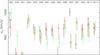 |
Fig. A.1 SIS model on the multi-modal SARCS candidates. The centre chosen for the shear profile is located either on the strong-lensing system (black open squares), at the middle of the 2 luminosity over-densities (red open circles) or on the luminosity peak not associated to the strong lensing features (green open triangles). The measured dispersion at the three different positionings can be used as an indicator of the dominance of the strong lens within its group. |
Acknowledgments
G.F. acknowledges support from FONDECYT through grant 3120160. V.M. acknowledges support from FONDECYT through grant 112074. M.L. acknowledges the Centre National de la Recherche Scientifique (CNRS) for its support. The Dark Cosmology Centre is funded by the Danish National Research Foundation. T.V. acknowledges support from CONACYT grant 165365 through the programme ÒEstancias posdoctorales y sabáticas al extranjero para la consolidación de grupos de investigación. R.G. acknowledges support from the Centre National des Estudes Spatiales. R.M. acknowledges support from CONICYT CATA-BASAL and FONDECYT through grant 3130750. G.F., V.M., M.L, and R.C. acknowledge support from ECOS-CONICYT C12U02. We acknowledge support from Programme National de Cosmologie (PNCG). Based on observations obtained with MEGAPRIME/MegaCam, a joint project of CFHT and CEA/DAPNIA, at the Canada-France-Hawaii Telescope (CFHT), which is operated by the National Research Council (NRC) of Canada, the Institut National des Science de l’Univers of the Centre National de la Recherche Scientifique (CNRS) of France, and the University of Hawaii. This work is based in part on data products produced at TERAPIX and the Canadian Astronomy Data Centre as part of the Canada-France-Hawaii Telescope Legacy Survey, a collaborative project of the NRC and CNRS.
References
- Akritas, M. G., & Bershady, M. A. 1996, ApJ, 470, 706 [NASA ADS] [CrossRef] [Google Scholar]
- Alard, C. 2006 [arXiv:astro-ph/0606757] [Google Scholar]
- Andreon, S., & Hurn, M. A. 2010, MNRAS, 404, 1922 [NASA ADS] [Google Scholar]
- Arnaud, M. 2005, in Background Microwave Radiation and Intracluster Cosmology, eds. F. Melchiorri, & Y. Rephaeli, 77 (The Netherlands: JOBS press and Bologna: Società Italiana di Fisica) [Google Scholar]
- Bahcall, N. A. 2000, Phys. Rep., 333, 233 [NASA ADS] [CrossRef] [Google Scholar]
- Bahcall, N. A., & Comerford, J. M. 2002, ApJ, 565, L5 [NASA ADS] [CrossRef] [Google Scholar]
- Balogh, M. L., Morris, S. L., Yee, H. K. C., Carlberg, R. G., & Ellingson, E. 1999, ApJ, 527, 54 [NASA ADS] [CrossRef] [Google Scholar]
- Balogh, M. L., Wilman, D., Henderson, R. D. E., et al. 2007, MNRAS, 374, 1169 [NASA ADS] [CrossRef] [Google Scholar]
- Balogh, M. L., Mazzotta, P., Bower, R. G., et al. 2011a, MNRAS, 412, 947 [NASA ADS] [CrossRef] [Google Scholar]
- Balogh, M. L., McGee, S. L., Wilman, D. J., et al. 2011b, MNRAS, 412, 2303 [Google Scholar]
- Bardeau, S., Kneib, J.-P., Czoske, O., et al. 2005, A&A, 434, 433 [NASA ADS] [CrossRef] [EDP Sciences] [Google Scholar]
- Bardeau, S., Soucail, G., Kneib, J.-P., et al. 2007, A&A, 470, 449 [NASA ADS] [CrossRef] [EDP Sciences] [Google Scholar]
- Becker, M. R., McKay, T. A., Koester, B., et al. 2007, ApJ, 669, 905 [NASA ADS] [CrossRef] [Google Scholar]
- Bekki, K. 1999, ApJ, 510, L15 [NASA ADS] [CrossRef] [Google Scholar]
- Bergé, J., Pacaud, F., Réfrégier, A., et al. 2008, MNRAS, 385, 695 [NASA ADS] [CrossRef] [Google Scholar]
- Berlind, A. A., Weinberg, D. H., Benson, A. J., et al. 2003, ApJ, 593, 1 [NASA ADS] [CrossRef] [Google Scholar]
- Bertin, E., & Arnouts, S. 1996, A&A, 117, 393 [Google Scholar]
- Biviano, A., Murante, G., Borgani, S., et al. 2006, A&A, 456, 23 [NASA ADS] [CrossRef] [EDP Sciences] [Google Scholar]
- Böhringer, H., Voges, W., Huchra, J. P., et al. 2000, ApJS, 129, 435 [NASA ADS] [CrossRef] [Google Scholar]
- Böhringer, H., Schuecker, P., Pratt, G. W., et al. 2007, A&A, 469, 363 [NASA ADS] [CrossRef] [EDP Sciences] [Google Scholar]
- Bolton, A. S., Burles, S., Koopmans, L. V. E., Treu, T., & Moustakas, L. A. 2006, ApJ, 638, 703 [NASA ADS] [CrossRef] [Google Scholar]
- Bolzonella, M., Miralles, J.-M., & Pelló, R. 2000, A&A, 363, 476 [NASA ADS] [Google Scholar]
- Bonamente, M., Joy, M., LaRoque, S. J., et al. 2008, ApJ, 675, 106 [NASA ADS] [CrossRef] [Google Scholar]
- Borgani, S., Murante, G., Springel, V., et al. 2004, MNRAS, 348, 1078 [NASA ADS] [CrossRef] [Google Scholar]
- Boselli, A., & Gavazzi, G. 2006, PASP, 118, 517 [NASA ADS] [CrossRef] [Google Scholar]
- Brainerd, T. G., Blandford, R. D., & Smail, I. 1996, ApJ, 466, 623 [NASA ADS] [CrossRef] [Google Scholar]
- Bridle, S., Gull, S., Bardeau, S., & Kneib, J.-P. 2002, in Proc. of the Yale Cosmology Workshop: The Shapes of Galaxies and their Dark Halos, 38 (World Scientific) [Google Scholar]
- Brough, S., Forbes, D. A., Kilborn, V. A., & Couch, W. 2006, MNRAS, 370, 1223 [NASA ADS] [CrossRef] [Google Scholar]
- Bruzual, G., & Charlot, S. 2003, MNRAS, 344, 1000 [NASA ADS] [CrossRef] [Google Scholar]
- Butcher, H., & Oemler, Jr., A. 1984, ApJ, 285, 426 [NASA ADS] [CrossRef] [Google Scholar]
- Cabanac, R. A., Alard, C., Dantel-Fort, M., et al. 2007, A&A, 461, 813 [NASA ADS] [CrossRef] [EDP Sciences] [Google Scholar]
- Carlstrom, J. E., Holder, G. P., & Reese, E. D. 2002, ARA&A, 40, 643 [NASA ADS] [CrossRef] [Google Scholar]
- Carollo, C. M., Cibinel, A., Lilly, S. J., et al. 2013, ApJ, 776, 71 [NASA ADS] [CrossRef] [Google Scholar]
- Cibinel, A., Carollo, C. M., Lilly, S. J., et al. 2013, ApJ, 777, 116 [NASA ADS] [CrossRef] [Google Scholar]
- Colless, M., Dalton, G., Maddox, S., et al. 2001, MNRAS, 328, 1039 [NASA ADS] [CrossRef] [Google Scholar]
- Connelly, J. L., Wilman, D. J., Finoguenov, A., et al. 2012, ApJ, 756, 139 [NASA ADS] [CrossRef] [Google Scholar]
- Coupon, J., Ilbert, O., Kilbinger, M., et al. 2009, A&A, 500, 981 [NASA ADS] [CrossRef] [EDP Sciences] [Google Scholar]
- Cowie, L. L., & Binney, J. 1977, ApJ, 215, 723 [NASA ADS] [CrossRef] [Google Scholar]
- Cucciati, O., Marinoni, C., Iovino, A., et al. 2010, A&A, 520, A42 [NASA ADS] [CrossRef] [EDP Sciences] [Google Scholar]
- Cypriano, E. S., Sodré, Jr., L., Kneib, J., & Campusano, L. E. 2004, ApJ, 613, 95 [NASA ADS] [CrossRef] [Google Scholar]
- De Lucia, G., Kauffmann, G., Springel, V., et al. 2004, MNRAS, 348, 333 [NASA ADS] [CrossRef] [Google Scholar]
- De Lucia, G., Poggianti, B. M., Aragón-Salamanca, A., et al. 2007, MNRAS, 374, 809 [NASA ADS] [CrossRef] [Google Scholar]
- Dietrich, J. P., Böhnert, A., Lombardi, M., Hilbert, S., & Hartlap, J. 2012, MNRAS, 419, 3547 [NASA ADS] [CrossRef] [Google Scholar]
- Dolag, K., Meneghetti, M., Moscardini, L., Rasia, E., & Bonaldi, A. 2006, MNRAS, 370, 656 [NASA ADS] [Google Scholar]
- Dressler, A., Oemler, Jr., A., Poggianti, B. M., et al. 2004, ApJ, 617, 867 [NASA ADS] [CrossRef] [Google Scholar]
- Ebeling, H., Edge, A. C., & Henry, J. P. 2001, ApJ, 553, 668 [Google Scholar]
- Eke, V. R., Baugh, C. M., Cole, S., et al. 2004, MNRAS, 348, 866 [NASA ADS] [CrossRef] [Google Scholar]
- Ellingson, E., Lin, H., Yee, H. K. C., & Carlberg, R. G. 2001, ApJ, 547, 609 [NASA ADS] [CrossRef] [Google Scholar]
- Ettori, S., Borgani, S., Moscardini, L., et al. 2004, MNRAS, 354, 111 [NASA ADS] [CrossRef] [Google Scholar]
- Evrard, A. E. 1990, ApJ, 363, 349 [NASA ADS] [CrossRef] [Google Scholar]
- Evrard, A. E., MacFarland, T. J., Couchman, H. M. P., et al. 2002, ApJ, 573, 7 [NASA ADS] [CrossRef] [Google Scholar]
- Evrard, A. E., Bialek, J., Busha, M., et al. 2008, ApJ, 672, 122 [NASA ADS] [CrossRef] [Google Scholar]
- Faltenbacher, A., Hoffman, Y., Gottlöber, S., & Yepes, G. 2007, MNRAS, 376, 1327 [NASA ADS] [CrossRef] [Google Scholar]
- Fassnacht, C. D., Kocevski, D. D., Auger, M. W., et al. 2008, ApJ, 681, 1017 [NASA ADS] [CrossRef] [Google Scholar]
- Finoguenov, A., Reiprich, T. H., & Böhringer, H. 2001, A&A, 368, 749 [NASA ADS] [CrossRef] [EDP Sciences] [Google Scholar]
- Finoguenov, A., Guzzo, L., Hasinger, G., et al. 2007a, ApJ, 172, 182 [Google Scholar]
- Finoguenov, A., Ponman, T. J., Osmond, J. P. F., & Zimer, M. 2007b, MNRAS, 374, 737 [NASA ADS] [CrossRef] [Google Scholar]
- Foëx, G., Soucail, G., Pointecouteau, E., et al. 2012, A&A, 546, A106 [NASA ADS] [CrossRef] [EDP Sciences] [Google Scholar]
- Fukugita, M., Ichikawa, T., Gunn, J. E., et al. 1996, AJ, 111, 1748 [NASA ADS] [CrossRef] [Google Scholar]
- Gao, L., White, S. D. M., Jenkins, A., Stoehr, F., & Springel, V. 2004, MNRAS, 355, 819 [NASA ADS] [CrossRef] [Google Scholar]
- Gastaldello, F., Buote, D. A., Humphrey, P. J., et al. 2007, ApJ, 669, 158 [NASA ADS] [CrossRef] [Google Scholar]
- Gavazzi, R., & Soucail, G. 2007, A&A, 462, 459 [NASA ADS] [CrossRef] [EDP Sciences] [Google Scholar]
- George, M. R., Leauthaud, A., Bundy, K., et al. 2012, ApJ, 757, 2 [NASA ADS] [CrossRef] [Google Scholar]
- Giodini, S., Pierini, D., Finoguenov, A., et al. 2009, ApJ, 703, 982 [NASA ADS] [CrossRef] [Google Scholar]
- Gladders, M. D., Hoekstra, H., Yee, H. K. C., Hall, P. B., & Barrientos, L. F. 2003, ApJ, 593, 48 [NASA ADS] [CrossRef] [Google Scholar]
- Gladders, M. D., & Yee, H. K. C. 2005, ApJS, 157, 1 [NASA ADS] [CrossRef] [Google Scholar]
- Haiman, Z., Mohr, J. J., & Holder, G. P. 2001, ApJ, 553, 545 [NASA ADS] [CrossRef] [Google Scholar]
- Hausman, M. A., & Ostriker, J. P. 1978, ApJ, 224, 320 [NASA ADS] [CrossRef] [Google Scholar]
- Helsdon, S. F., & Ponman, T. J. 2000, MNRAS, 315, 356 [NASA ADS] [CrossRef] [Google Scholar]
- Helsdon, S. F., & Ponman, T. J. 2003a, MNRAS, 339, L29 [NASA ADS] [CrossRef] [Google Scholar]
- Helsdon, S. F., & Ponman, T. J. 2003b, MNRAS, 340, 485 [NASA ADS] [CrossRef] [Google Scholar]
- Heymans, C., Van Waerbeke, L., Bacon, D., et al. 2006, MNRAS, 368, 1323 [NASA ADS] [CrossRef] [Google Scholar]
- Hoekstra, H. 2007, MNRAS, 379, 317 [NASA ADS] [CrossRef] [Google Scholar]
- Hoekstra, H., Franx, M., & Kuijken, K. 2000, ApJ, 532, 88 [NASA ADS] [CrossRef] [Google Scholar]
- Hoekstra, H., Hartlap, J., Hilbert, S., & van Uitert, E. 2011, MNRAS, 412, 2095 [NASA ADS] [CrossRef] [Google Scholar]
- Hoekstra, H., Mahdavi, A., Babul, A., & Bildfell, C. 2012, MNRAS, 427, 1298 [NASA ADS] [CrossRef] [Google Scholar]
- Huertas-Company, M., Foex, G., Soucail, G., & Pelló, R. 2009, A&A, 505, 83 [NASA ADS] [CrossRef] [EDP Sciences] [Google Scholar]
- Ienna, F. & Pelló, R. 2006, in SF2A-2006: Semaine de l’Astrophysique Francaise, eds. D. Barret, F. Casoli, G. Lagache, A. Lecavelier, & L. Pagani, 347 [Google Scholar]
- Ivezic, Z., Tyson, J. A., Acosta, E., et al. 2008 [arXiv:0805.2366] [Google Scholar]
- Jauzac, M., Jullo, E., Kneib, J.-P., et al. 2012, MNRAS, 426, 3369 [Google Scholar]
- Jeltema, T. E., Mulchaey, J. S., Lubin, L. M., Rosati, P., & Böhringer, H. 2006, ApJ, 649, 649 [NASA ADS] [CrossRef] [Google Scholar]
- Jeltema, T. E., Mulchaey, J. S., Lubin, L. M., & Fassnacht, C. D. 2007, ApJ, 658, 865 [NASA ADS] [CrossRef] [Google Scholar]
- Johnston, D. E., Sheldon, E. S., Wechsler, R. H., et al. 2007 [arXiv:0709.1159] [Google Scholar]
- Jullo, E., Kneib, J., Limousin, M., et al. 2007, New J. Phys., 9, 447 [Google Scholar]
- Kaiser, N. 1986, MNRAS, 222, 323 [NASA ADS] [CrossRef] [Google Scholar]
- Kneib, J., Ellis, R. S., Smail, I., Couch, W. J., & Sharples, R. M. 1996, ApJ, 471, 643 [NASA ADS] [CrossRef] [Google Scholar]
- Knobel, C., Lilly, S. J., Iovino, A., et al. 2009, ApJ, 697, 1842 [NASA ADS] [CrossRef] [Google Scholar]
- Kodama, T., Yamada, T., Akiyama, M., et al. 2004, MNRAS, 350, 1005 [NASA ADS] [CrossRef] [Google Scholar]
- Koester, B. P., McKay, T. A., Annis, J., et al. 2007a, ApJ, 660, 239 [NASA ADS] [CrossRef] [Google Scholar]
- Koester, B. P., McKay, T. A., Annis, J., et al. 2007b, ApJ, 660, 221 [NASA ADS] [CrossRef] [Google Scholar]
- Kotov, O., & Vikhlinin, A. 2005, ApJ, 633, 781 [NASA ADS] [CrossRef] [Google Scholar]
- Kravtsov, A. V., Berlind, A. A., Wechsler, R. H., et al. 2004, ApJ, 609, 35 [NASA ADS] [CrossRef] [Google Scholar]
- Lancaster, K., Birkinshaw, M., Gawroński, M. P., et al. 2011, MNRAS, 418, 1441 [NASA ADS] [CrossRef] [Google Scholar]
- Lau, E. T., Nagai, D., & Kravtsov, A. V. 2010, ApJ, 708, 1419 [NASA ADS] [CrossRef] [Google Scholar]
- Leauthaud, A., Finoguenov, A., Kneib, J., et al. 2010, ApJ, 709, 97 [NASA ADS] [CrossRef] [Google Scholar]
- Limousin, M., Kneib, J. P., Bardeau, S., et al. 2007a, A&A, 461, 881 [NASA ADS] [CrossRef] [EDP Sciences] [Google Scholar]
- Limousin, M., Richard, J., Jullo, E., et al. 2007b, ApJ, 668, 643 [NASA ADS] [CrossRef] [Google Scholar]
- Limousin, M., Cabanac, R., Gavazzi, R., et al. 2009, A&A, 502, 445 [NASA ADS] [CrossRef] [EDP Sciences] [Google Scholar]
- Limousin, M., Ebeling, H., Ma, C., et al. 2010a, MNRAS, 405, 777 [NASA ADS] [Google Scholar]
- Limousin, M., Jullo, E., Richard, J., et al. 2010b, A&A, 524, A95 [NASA ADS] [CrossRef] [EDP Sciences] [Google Scholar]
- Lin, Y., Mohr, J. J., & Stanford, S. A. 2003, ApJ, 591, 749 [NASA ADS] [CrossRef] [Google Scholar]
- Lin, Y., Mohr, J. J., & Stanford, S. A. 2004, ApJ, 610, 745 [NASA ADS] [CrossRef] [Google Scholar]
- Lubin, L. M., Oke, J. B., & Postman, M. 2002, AJ, 124, 1905 [NASA ADS] [CrossRef] [Google Scholar]
- Lubin, L. M., Gal, R. R., Lemaux, B. C., Kocevski, D. D., & Squires, G. K. 2009, AJ, 137, 4867 [NASA ADS] [CrossRef] [Google Scholar]
- Luppino, G. A., Gioia, I. M., Hammer, F., Le Fèvre, O., & Annis, J. A. 1999, A&AS, 136, 117 [NASA ADS] [CrossRef] [EDP Sciences] [Google Scholar]
- Mahdavi, A., Hoekstra, H., Babul, A., et al. 2013, ApJ, 767, 116 [NASA ADS] [CrossRef] [Google Scholar]
- Mamon, G. A. 2007, in Groups of Galaxies in the Nearby Universe, eds. I. Saviane, V. D. Ivanov, & J. Borissova, 203 (Springer Verlag) [Google Scholar]
- Mandelbaum, R., Seljak, U., Cool, R. J., et al. 2006, MNRAS, 372, 758 [NASA ADS] [CrossRef] [Google Scholar]
- Mandelbaum, R., Seljak, U., Hirata, C. M., et al. 2008, MNRAS, 386, 781 [NASA ADS] [CrossRef] [Google Scholar]
- Mandelbaum, R., Seljak, U., Baldauf, T., & Smith, R. E. 2010, MNRAS, 405, 2078 [NASA ADS] [Google Scholar]
- Marian, L., & Bernstein, G. M. 2006, Phys. Rev. D, 73, 123525 [NASA ADS] [CrossRef] [Google Scholar]
- Marinoni, C., & Hudson, M. J. 2002, ApJ, 569, 101 [NASA ADS] [CrossRef] [Google Scholar]
- Marrone, D. P., Smith, G. P., Richard, J., et al. 2009, ApJ, 701, L114 [NASA ADS] [CrossRef] [Google Scholar]
- Massey, R., Rhodes, J., Ellis, R., et al. 2007, Nature, 445, 286 [NASA ADS] [CrossRef] [PubMed] [Google Scholar]
- McCarthy, I. G., Babul, A., Holder, G. P., & Balogh, M. L. 2003, ApJ, 591, 515 [NASA ADS] [CrossRef] [Google Scholar]
- Miller, C. J., Nichol, R. C., Reichart, D., et al. 2005, AJ, 130, 968 [Google Scholar]
- Morandi, A., Ettori, S., & Moscardini, L. 2007, MNRAS, 379, 518 [NASA ADS] [CrossRef] [Google Scholar]
- More, A., Jahnke, K., More, S., et al. 2011, ApJ, 734, 69 [NASA ADS] [CrossRef] [Google Scholar]
- More, A., Cabanac, R., More, S., et al. 2012, ApJ, 749, 38 [Google Scholar]
- Muñoz, J. A., Falco, E. E., Kochanek, C. S., et al. 1998, Ap&SS, 263, 51 [NASA ADS] [CrossRef] [Google Scholar]
- Muñoz, R. P., Motta, V., Verdugo, T., et al. 2013, A&A, 552, A80 [NASA ADS] [CrossRef] [EDP Sciences] [Google Scholar]
- Mulchaey, J. S., & Zabludoff, A. I. 1998, ApJ, 496, 73 [NASA ADS] [CrossRef] [Google Scholar]
- Mulchaey, J. S., Lubin, L. M., Fassnacht, C., Rosati, P., & Jeltema, T. E. 2006, ApJ, 646, 133 [NASA ADS] [CrossRef] [Google Scholar]
- Muzzin, A., Yee, H. K. C., Hall, P. B., & Lin, H. 2007, ApJ, 663, 150 [NASA ADS] [CrossRef] [Google Scholar]
- Myers, S. T., Jackson, N. J., Browne, I. W. A., et al. 2003, MNRAS, 341, 1 [NASA ADS] [CrossRef] [Google Scholar]
- Navarro, J. F., Frenk, C. S., & White, S. D. M. 1997, ApJ, 490, 493 [NASA ADS] [CrossRef] [Google Scholar]
- Navarro, J. F., Hayashi, E., Power, C., et al. 2004, MNRAS, 349, 1039 [NASA ADS] [CrossRef] [Google Scholar]
- Oguri, M. 2006, MNRAS, 367, 1241 [NASA ADS] [CrossRef] [Google Scholar]
- Oguri, M., Hennawi, J. F., Gladders, M. D., et al. 2009, ApJ, 699, 1038 [NASA ADS] [CrossRef] [Google Scholar]
- Oguri, M., Bayliss, M. B., Dahle, H., et al. 2012, MNRAS, 420, 3213 [NASA ADS] [CrossRef] [Google Scholar]
- Okabe, N., & Umetsu, K. 2008, PASJ, 60, 345 [NASA ADS] [Google Scholar]
- Okabe, N., Takada, M., Umetsu, K., Futamase, T., & Smith, G. P. 2010, PASJ, 62, 811 [NASA ADS] [Google Scholar]
- Osmond, J. P. F., & Ponman, T. J. 2004, MNRAS, 350, 1511 [NASA ADS] [CrossRef] [Google Scholar]
- Ostriker, J. P., & Tremaine, S. D. 1975, ApJ, 202, L113 [NASA ADS] [CrossRef] [Google Scholar]
- Pandey, B., & Bharadwaj, S. 2006, MNRAS, 372, 827 [NASA ADS] [CrossRef] [Google Scholar]
- Parker, L. C., Hudson, M. J., Carlberg, R. G., & Hoekstra, H. 2005, ApJ, 634, 806 [NASA ADS] [CrossRef] [Google Scholar]
- Pimbblet, K. A., Drinkwater, M. J., & Hawkrigg, M. C. 2004, MNRAS, 354, L61 [NASA ADS] [CrossRef] [Google Scholar]
- Planck Collaboration 2011a, A&A, 536, A8 [NASA ADS] [CrossRef] [EDP Sciences] [Google Scholar]
- Planck Collaboration 2011b, A&A, 536, A11 [NASA ADS] [CrossRef] [EDP Sciences] [Google Scholar]
- Planck Collaboration 2011c, A&A, 536, A10 [NASA ADS] [CrossRef] [EDP Sciences] [Google Scholar]
- Poggianti, B. 2004, in Baryons in Dark Matter Halos, eds. R. Dettmar, U. Klein, & P. Salucci, Proc. Sci., 104 [Google Scholar]
- Poggianti, B. M., von der Linden, A., De Lucia, G., et al. 2006, ApJ, 642, 188 [NASA ADS] [CrossRef] [Google Scholar]
- Popesso, P., Biviano, A., Böhringer, H., Romaniello, M., & Voges, W. 2005, A&A, 433, 431 [NASA ADS] [CrossRef] [EDP Sciences] [Google Scholar]
- Popesso, P., Biviano, A., Böhringer, H., & Romaniello, M. 2007, A&A, 464, 451 [NASA ADS] [CrossRef] [EDP Sciences] [Google Scholar]
- Pratt, G. W., Croston, J. H., Arnaud, M., & Böhringer, H. 2009, A&A, 498, 361 [NASA ADS] [CrossRef] [EDP Sciences] [Google Scholar]
- Quintana, H., & Lawrie, D. G. 1982, AJ, 87, 1 [NASA ADS] [CrossRef] [Google Scholar]
- Radovich, M., Puddu, E., Romano, A., Grado, A., & Getman, F. 2008, A&A, 487, 55 [NASA ADS] [CrossRef] [EDP Sciences] [Google Scholar]
- Rasmussen, J., & Ponman, T. J. 2007, MNRAS, 380, 1554 [NASA ADS] [CrossRef] [Google Scholar]
- Reyes, R., Mandelbaum, R., Hirata, C., Bahcall, N., & Seljak, U. 2008, MNRAS, 390, 1157 [NASA ADS] [CrossRef] [Google Scholar]
- Rozo, E., Rykoff, E. S., Evrard, A., et al. 2009, ApJ, 699, 768 [NASA ADS] [CrossRef] [Google Scholar]
- Ruff, A. J., Gavazzi, R., Marshall, P. J., et al. 2011, ApJ, 727, 96 [NASA ADS] [CrossRef] [Google Scholar]
- Rykoff, E. S., Evrard, A. E., McKay, T. A., et al. 2008, MNRAS, 387, L28 [NASA ADS] [Google Scholar]
- Scoville, N., Aussel, H., Brusa, M., et al. 2007, ApJS, 172, 1 [NASA ADS] [CrossRef] [Google Scholar]
- Seitz, C., & Schneider, P. 1997, A&A, 318, 687 [NASA ADS] [Google Scholar]
- Skibba, R. A., van den Bosch, F. C., Yang, X., et al. 2011, MNRAS, 410, 417 [NASA ADS] [CrossRef] [Google Scholar]
- Smail, I., Edge, A. C., Ellis, R. S., & Blandford, R. D. 1998, MNRAS, 293, 124 [NASA ADS] [CrossRef] [Google Scholar]
- Soucail, G. 2012, A&A, 540, A61 [NASA ADS] [CrossRef] [EDP Sciences] [Google Scholar]
- Springel, V., & Hernquist, L. 2003, MNRAS, 339, 312 [NASA ADS] [CrossRef] [Google Scholar]
- Springel, V., White, S. D. M., Jenkins, A., et al. 2005, Nature, 435, 629 [NASA ADS] [CrossRef] [PubMed] [Google Scholar]
- Staniszewski, Z., Ade, P. A. R., Aird, K. A., et al. 2009, ApJ, 701, 32 [CrossRef] [Google Scholar]
- Stott, J. P., Pimbblet, K. A., Edge, A. C., Smith, G. P., & Wardlow, J. L. 2009, MNRAS, 394, 2098 [NASA ADS] [CrossRef] [Google Scholar]
- Sun, M., Voit, G. M., Donahue, M., et al. 2009, ApJ, 693, 1142 [NASA ADS] [CrossRef] [Google Scholar]
- Thanjavur, K., Crampton, D., & Willis, J. 2010, ApJ, 714, 1355 [NASA ADS] [CrossRef] [Google Scholar]
- Tran, K.-V. H., Franx, M., Illingworth, G., Kelson, D. D., & van Dokkum, P. 2003, ApJ, 599, 865 [NASA ADS] [CrossRef] [Google Scholar]
- Treu, T., Ellis, R. S., Kneib, J., et al. 2003, ApJ, 591, 53 [NASA ADS] [CrossRef] [Google Scholar]
- Verdugo, T., Motta, V., Muñoz, R. P., et al. 2011, A&A, 527, A124 [NASA ADS] [CrossRef] [EDP Sciences] [Google Scholar]
- Vikhlinin, A., van Speybroeck, L., Markevitch, M., Forman, W. R., & Grego, L. 2002, ApJ, 578, L107 [NASA ADS] [CrossRef] [Google Scholar]
- Vikhlinin, A., Kravtsov, A., Forman, W., et al. 2006, ApJ, 640, 691 [NASA ADS] [CrossRef] [Google Scholar]
- Vikhlinin, A., Kravtsov, A. V., Burenin, R. A., et al. 2009, ApJ, 692, 1060 [NASA ADS] [CrossRef] [Google Scholar]
- Voit, G. M. 2005, Rev. Mod. Phys., 77, 207 [NASA ADS] [CrossRef] [Google Scholar]
- Wang, S., Khoury, J., Haiman, Z., & May, M. 2004, Phys. Rev. D, 70, 123008 [NASA ADS] [CrossRef] [Google Scholar]
- Wen, Z.-L., Han, J.-L., & Jiang, Y.-Y. 2011, Res. Astron. Astrophys., 11, 1185 [NASA ADS] [CrossRef] [Google Scholar]
- White, S. D. M., & Frenk, C. S. 1991, ApJ, 379, 52 [NASA ADS] [CrossRef] [Google Scholar]
- White, S. D. M., Navarro, J. F., Evrard, A. E., & Frenk, C. S. 1993, Nature, 366, 429 [NASA ADS] [CrossRef] [Google Scholar]
- White, M., Hernquist, L., & Springel, V. 2001, ApJ, 550, L129 [NASA ADS] [CrossRef] [Google Scholar]
- Willis, J. P., Pacaud, F., Valtchanov, I., et al. 2005, MNRAS, 363, 675 [NASA ADS] [CrossRef] [Google Scholar]
- Wilman, D. J., Oemler, Jr., A., Mulchaey, J. S., et al. 2009, ApJ, 692, 298 [NASA ADS] [CrossRef] [Google Scholar]
- Yang, X., Mo, H. J., & van den Bosch, F. C. 2008, ApJ, 676, 248 [Google Scholar]
- Zabludoff, A. I., & Mulchaey, J. S. 1998, ApJ, 496, 39 [NASA ADS] [CrossRef] [Google Scholar]
- Zabludoff, A. I., & Mulchaey, J. S. 2000, ApJ, 539, 136 [NASA ADS] [CrossRef] [Google Scholar]
- Zaritsky, D., & Gonzalez, A. H. 2003, ApJ, 584, 691 [NASA ADS] [CrossRef] [Google Scholar]
All Tables
Summary of the fitting results for the scaling relations (σ/σ0) = A × (Obs./PObs.)α.
All Figures
|
Fig. 1 Shear profile for the candidate SA66 (σSIS = 644 km s-1, z_spec = 0.35). The black filled squares shows the tangential component of the shear, the blue open circles the B-mode of one of the shifted profiles (for clarity). The red curve is the SIS best fit to the tangential shear. |
| In the text | |
|
Fig. 2 Spectroscopic redshifts versus photometric redshifts for the SARCS objects (see Table 2). The solid line shows the equality, the two dashed lines are at ± 0.1, i.e. a typical uncertainty on photometric redshifts. |
| In the text | |
|
Fig. 3 Variation in the average geometrical factor ⟨ Dls/Ds ⟩ as a function of the shift around the true lens redshift for three groups, SA48 (red curve), SA50 (green curve), and SA123 (blue curve). The two vertical dashed lines mark the typical ± 0.1uncertainty of photometric redshifts. |
| In the text | |
|
Fig. 4 Velocity dispersion derived from the fit of the shear profile using the SIS model. Red open triangles show the upper limit on σv for those objects not having a 1σ weak-lensing detection. Open circles are candidates with a weak-lensing detection less than 3σ, filled circles are those having a reliable detection (above 3σ). |
| In the text | |
|
Fig. 5 Richnesses estimated within 1 Mpc using the bright red galaxies of the 126 SARCS candidates. Open red triangles are objects without a 1σ weak-lensing detection, open circles have a detection between 1 and 3σ, filled circles are those with a detection above 3σ. |
| In the text | |
|
Fig. 6 Same as Fig. 5 for the optical i′-band luminosities estimated within 1 Mpc using the bright red galaxies of the 126 SARCS candidates. |
| In the text | |
|
Fig. 7 Luminosity density contours (in black) for SA15 equal to 106, 4 × 10⁶, 7 × 10⁶, 107, and 1.3 × 10⁷ L⊙ kpc-2. The white cross marks the galaxy at the centre of the strong-lensing system. The black vertical line on the left is 1 Mpc long. SA15 is at z = 0.44. The stamp in the top-right corner shows a 30′′ × 30′′ colour image of the system. |
| In the text | |
|
Fig. 8 Luminosity density contours (in black) for SA2 equal to 2 × 10⁶, 4 × 10⁶, 7 × 10⁶, 1.5 × 10⁷, and 2 × 10⁷ L⊙ kpc-2. The white cross marks the galaxy at the centre of the strong-lensing system. The black vertical line on the left is 1 Mpc long. SA2 is at z = 0.48. The stamp in the top-right corner shows a 30′′ × 30′′ colour image of the system. |
| In the text | |
|
Fig. 9 Luminosity density contours (in black) for SA90 equal to 1.5 × 10⁶, 4 × 10⁶, 7 × 10⁶, 107, and 1.5 × 10⁷ L⊙ kpc-2. The white cross marks the galaxy at the centre of the strong-lensing system. The black vertical line on the left is 1 Mpc long. SA90 is at z = 0.53. The stamp in the top-right corner shows a 30′′ × 30′′ colour image of the system. |
| In the text | |
|
Fig. 10 Velocity dispersion derived from weak lensing as a function of optical richness (first row) and luminosity (second row) estimated with the bright red galaxies in 2 apertures, 0.5 Mpc (left column) and 1 Mpc (right column). We used only the sample of the 80 candidates defined in Sect. 5.1 (error bars on each individual measurement are omitted for clarity, see Table 2). Green points with error bars highlight the increase in σv with richness and luminosity after binning the SARCS lenses according to their observed richness or luminosity. |
| In the text | |
|
Fig. 11 Richness-velocity dispersion scaling relation. The black solid line shows the best BCES orthogonal fit of the N1 Mpc − σSIS relation using the SARCS most secure candidates (red points) and adding the EXCPRES galaxy clusters of Foëx et al. (2012) (blue open triangles). The grey shaded area gives the statistical 1σ uncertainty given by the best fit parameters (statistical dispersion σstat). The red line (and corresponding shaded area) is the best fit using only the SARCS most secure candidates. |
| In the text | |
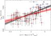 |
Fig. 12 Same as Fig. 11 but for the luminosity-velocity dispersion scaling relation. |
| In the text | |
|
Fig. A.1 SIS model on the multi-modal SARCS candidates. The centre chosen for the shear profile is located either on the strong-lensing system (black open squares), at the middle of the 2 luminosity over-densities (red open circles) or on the luminosity peak not associated to the strong lensing features (green open triangles). The measured dispersion at the three different positionings can be used as an indicator of the dominance of the strong lens within its group. |
| In the text | |
Current usage metrics show cumulative count of Article Views (full-text article views including HTML views, PDF and ePub downloads, according to the available data) and Abstracts Views on Vision4Press platform.
Data correspond to usage on the plateform after 2015. The current usage metrics is available 48-96 hours after online publication and is updated daily on week days.
Initial download of the metrics may take a while.