| Issue |
A&A
Volume 558, October 2013
|
|
|---|---|---|
| Article Number | A69 | |
| Number of page(s) | 16 | |
| Section | Interstellar and circumstellar matter | |
| DOI | https://doi.org/10.1051/0004-6361/201322087 | |
| Published online | 04 October 2013 | |
Dense molecular cocoons in the massive protocluster W3 IRS5: a test case for models of massive star formation
1 Leiden Observatory, Leiden University, PO Box 9513, 2300 RA Leiden, The Netherlands
e-mail: This email address is being protected from spambots. You need JavaScript enabled to view it.
2 Harvard-Smithsonian Center for Astrophysics, 60 Garden Street, Cambridge, MA 02138, USA
3 SRON Netherlands Institute for Space Research, Landleven 12, 9747 AD, 9712 Groningen, The Netherlands
4 Kapteyn Astronomical Institute, University of Groningen, 9712 Groningen, The Netherlands
5 Institute of Astronomy, ETH Zürich, 8093 Zürich, Switzerland
6 Ritter Observatory, MS-113, University of Toledo, 2801 W. Bancroft St., Toledo, OH 43606, USA
7 Naval Research Laboratory, Code 7210, Washington, DC 20375, USA
Received: 14 June 2013
Accepted: 21 August 2013
Abstract
Context. Two competing models describe the formation of massive stars in objects like the Orion Trapezium. In the turbulent core accretion model, the resulting stellar masses are directly related to the mass distribution of the cloud condensations. In the competitive accretion model, the gravitational potential of the protocluster captures gas from the surrounding cloud for which the individual cluster members compete.
Aims. With high resolution submillimeter observations of the structure, kinematics, and chemistry of the proto-Trapezium cluster W3 IRS5, we aim to determine which mode of star formation dominates.
Methods. We present 354 GHz Submillimeter Array observations at resolutions of 1″–3″ (1800–5400 AU) of W3 IRS5. The dust continuum traces the compact source structure and masses of the individual cores, while molecular lines of CS, SO, SO2, HCN, H2CS, HNCO, and CH3OH (and isotopologues) reveal the gas kinematics, density, and temperature.
Results. The observations show five emission peaks (SMM1–5). SMM1 and SMM2 contain massive embedded stars (~20 M⊙); SMM3–5 are starless or contain low-mass stars (<8 M⊙). The inferred densities are high, ≥107 cm-3, but the core masses are small, 0.2−0.6 M⊙. The detected molecular emission reveals four different chemical zones. Abundant (X ~ few 10-7 to 10-6) SO and SO2 are associated with SMM1 and SMM2, indicating active sulfur chemistry. A low abundance (5 × 10⁻⁸) of CH3OH concentrated on SMM3/4 suggest the presence of a hot core that is only just turning on, possibly by external feedback from SMM1/2. The gas kinematics are complex with contributions from a near pole-on outflow traced by CS, SO, and HCN; rotation in SO2, and a jet in vibrationally excited HCN.
Conclusions. The proto-Trapezium cluster W3 IRS5 is an ideal test case to discriminate between models of massive star formation. Either the massive stars accrete locally from their local cores; in this case the small core masses imply that W3 IRS5 is at the very end stages (1000 yr) of infall and accretion, or the stars are accreting from the global collapse of a massive, cluster forming core. We find that the observed masses, densities and line widths observed toward W3 IRS 5 and the surrounding cluster forming core are consistent with the competitive accretion of gas at rates of Ṁ ~ 10-4M⊙ yr-1 by the massive young forming stars. Future mapping of the gas kinematics from large to small scales will determine whether large-scale gas inflow occurs and how the cluster members compete to accrete this material.
Key words: stars: massive / stars: formation / ISM: kinematics and dynamics / ISM: individual objects: W3 IRS5
© ESO, 2013
1. Introduction
In contrast to low-mass star formation, there is no single agreed upon scenario for the formation of massive stars (Zinnecker & Yorke 2007). Current models either predict that a turbulent core collapses into a cluster of stars of different mass (e.g. McKee & Tan 2003), or that multiple low-mass stars compete for the same mass reservoir, with a few winning and growing to become massive stars while most others remain low-mass stars (e.g. Bonnell et al. 2001; Bonnell & Bate 2006). Both theories are supported by observations (e.g. Cesaroni et al. 1997; Pillai et al. 2011), suggesting that there may be two different modes of massive star formation (Krumholz & Bonnell 2009). However, it is challenging to observe massive star-forming regions since they are at large distances (a few kpc), requiring high-angular resolution to resolve the highly embedded complex structures in which gravitational fragmentation, powerful outflows and stellar winds, and ionizing radiation fields play influence the star-formation processes (Beuther et al. 2007).
Although observationally challenging, progress in testing the models of massive star formation has been made recently with at centimeter, and (sub)millimeter wavelengths. Based on observations of the protocluster NGC 2264 with the IRAM 30 m telescope, Peretto et al. (2006) proposed a mixed type of star formation as proposed by Bonnell et al. (2001) and Bonnell & Bate (2006), and McKee & Tan (2003), where the turbulent, massive star-forming core is formed by the gravitational merger of lower mass cores at the center of a collapsing protocluster. Observations of G8.68–0.37 with the Submillimeter Array (SMA) and the Australia Telescope Compact Array (ATCA) imply that to form an O star, the star-forming core must continuously gain mass by accretion from a larger mass reservoir since protostellar heating from the low-mass stars is not sufficient to halt fragmentation (Longmore et al. 2011). Multi-wavelength observations of G29.96–0.02 and G35.20–1.74 suggest that the mass of massive star-forming cores is not limited to the natal cores formed by fragmentation and turbulence is not strong enough to prevent collapse, which favors the competitive accretion model (Pillai et al. 2011). On the other hand, Very Large Array (VLA) observations of IRAS 05345+3157 (Fontani et al. 2012) suggest that turbulence is an important factor in the initial fragmentation of the parental clump and is strong enough to provide support against further fragmentation down to thermal Jeans masses.
W3 IRS5 is a massive star-forming region located in the Perseus arm at a distance of 1.83 ± 0.14 kpc (Imai et al. 2000) with a total luminosity of 2 × 10⁵ L⊙ (Campbell et al. 1995). A cluster of hypercompact (<240 AU) H II regions are found from high-resolution cm-wavelength observations (Claussen et al. 1994; Wilson et al. 2003; van der Tak et al. 2005). Based on observations at near-IR wavelengths, Megeath et al. (1996, 2005, 2008) found a high stellar surface density of ~10 000 pc-2 and proposed that W3 IRS5 is a Trapezium cluster (Abt & Corbally 2000) in the making. A high protostellar number density exceeding 106 protostars pc-3 is also concluded by Rodón et al. (2008) from their 1.4 mm observations with the Plateau de Bure Interferometer (PdBI). The proximity and the dense protostellar environment make W3 IRS5 an excellent target to study massive star formation in a highly clustered mode.
(Sub)millimeter observations show that the molecular structure of W3 IRS5 is physically and chemically complex. Multiple bipolar outflows with various orientations are reported via different tracers (e.g. Mitchell et al. 1992; Ridge & Moore 2001; Gibb et al. 2007; Rodón et al. 2008; Wang et al. 2012). Although the outflow driving sources are not determined unambiguously, the infrared pair NIR1 and NIR2 (Megeath et al. 2005) are likely candidates. The detection of near-IR and X-ray emission toward W3 IRS5 (Megeath et al. 2005; Hofner et al. 2002) likely benefits from an outflow oriented near the line of sight. A velocity gradient in the NW–SE direction on scales of a few arcseconds is seen in SO2, which may indicate rotation of the common envelope of NIR1 and NIR2 (Rodón et al. 2008; Wang et al. 2012). At 14″ resolution, many molecular species are detected toward W3 IRS5, especially sulfur-bearing molecules (Helmich et al. 1994; Helmich & van Dishoeck 1997), implying active hot-core chemistry (e.g. Charnley 1997) or shocks (e.g. Pineau des Forets et al. 1993). The sulfur-bearing species SO and SO2 peak near NIR1/NIR2, while complex organic molecules such as CH3CN and CH3OH peak at offset positions (Rodón et al. 2008; Wang et al. 2012).
This paper presents SMA observations of W3 IRS5 at 354 GHz with an angular resolution of 1″–3″, revealing the complex molecular environment of the proto-Trapezium cluster and tracing the star formation processes in the dense cluster-forming core. The observations and data calibration are summarized in Sect. 2. We present the observational results in Sect. 3, followed by data analysis in Sect. 4. We discuss our findings in Sect. 5, and conclude this paper in Sect. 6.
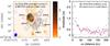 |
Fig. 1 a) Continuum emission of W3 IRS5 region at 353.6 GHz (black contours) overplotted with the NICMOS 2.22 μm emission (color scale). The synthesized beam size is |
Characteristics of the continuum emission in W3 IRS5 at 353.6 GHz.
2. Observations and data reduction
W3 IRS5 was observed with the SMA1 (Ho et al. 2004) on 2008 January 7 in the compact configuration and on 2006 January 15 in the extended configuration. Both observations were conducted with 7 antennas and were centered on  , δ(2000) = 62°05′52
 50. The weather conditions were good with τ225 GHz ~ 0.1. The reference VLSR was set to − 39.0 km s-1. The receiver was tuned to 353.741 GHz in the upper sideband, covering frequencies from 342.6 to 344.6 GHz and from 352.6 to 354.6 GHz. The correlator was configured to sample each spectral window by 256 channels, resulting a velocity resolution of ~0.35 km s-1 per channel. For the compact configuration dataset, 3C 454.3 was observed as bandpass calibrator. Gain calibration was performed by frequent observations of two quasars, 0136+478 (~ 16° away from the source) and 3C 84 (~22° away from the source). Uranus was adopted as absolute flux calibrator. For the extended configuration dataset, 3C 273, 3C 84 and 3C 273 were observed, respectively, as bandpass, gain and flux calibrators. The adopted total flux density of 3C 273 is 9.6 Jy, which is the mean value reported for five observations2 during 2006 January 13–30. We estimate that the uncertainty in absolute flux density is about 20%. The uv-range sampled by the combined dataset is 10 kλ (21″) to 210 kλ (1″).
Data reduction was conducted by using the MIR package (Scoville et al. 1993) adapted for the SMA, while imaging and analysis were performed in MIRIAD (Sault et al. 1995). To avoid line contamination, line-free channels were selected to separate the continuum and line emission in the visibility domain. The continuum visibilities for each dataset were self-calibrated using the brightest clean components to enhance the signal-to-noise ratio (S/N). Self-calibrated datasets were combined to image the continuum. To optimize sensitivity and angular resolution, a robust weighting3 parameter of 0.25 was adopted for the continuum imaging, resulting in a 1σ rms noise of 10 mJy per 1″ beam. Line identification was conducted by using the compact configuration dataset only with the aid of spectroscopy databases of JPL4 (Pickett et al. 1998) and CDMS5 (Müller et al. 2005). For those lines that were also clearly detected in the extended-configuration dataset, we imaged the combined compact+extended dataset.
3. Observational results
3.1. Continuum emission
Detected molecular transitions in W3 IRS5.
Figure 1 shows the continuum image and visibilities at 353.6 GHz. At a resolution of  and PA−14°, five major emission peaks, SMM1 to SMM5, were identified based on their relative intensities and a cutoff of 9σ. We note that irregular, extended emission is also observed around the identified peaks. More emission peaks may be present in the diffuse surroundings, which requires better sensitivity, angular resolution, and image fidelity for confirmation. The total flux density recorded by the SMA is about 2.5 Jy which is about 6% of the flux contained in the SCUBA image at 850 μm (Wang et al. 2012). To derive the positions and flux densities of the emission peaks, we fitted the data with five point sources in the visibility domain (Fig. 1b). The properties of the five sources are summarized in Table 1. With this simplified model, about half of the observed flux originates from the unresolved sources, while the extended emission detected in baselines of 10–25 kλ contributes the other half. The fit deviates significantly from the data at long baselines (>150 kλ) and on short baselines (<20 kλ). The former corresponds to fine image detail that we could fit by adding more point sources, but we find that the S/N does not warrant additional “sources”. The latter indicates that on scales >8″ there is significant emission that our 5-point model does not represent properly. An extended, Gaussian envelope could match these observations. However, on even larger spatial scales our uv sampling misses even larger amounts of emission. Therefore, we do not aim to model this extended emission, but instead refer to the SCUBA 850 μm emission to trace this component.
Table 1 lists the cm-wave, (sub)mm and IR sources associated with SMM1–5 (Claussen et al. 1994; Wilson et al. 2003; van der Tak et al. 2005; Megeath et al. 2005; Rodón et al. 2008; Wang et al. 2012). In Fig. 1a, we see that the emission decreases between SMM1/SMM2 and SMM3/SMM4/SMM5, dividing the cloud into two regions with the eastern part containing clusters of IR and cm-wave emission as well as X-ray emission (Hofner et al. 2002), while the western part shows no IR and cm-wave sources. This dichotomy implies that the eastern part of the source is more evolved and less embedded than the western part. We note that the projected positions of SMM1, SMM2 and SMM3 are aligned nearly in a straight line which could be the result of fragmentation at the scale of 1′′–2′′ (~1800–3600 AU), although this may be a projection effect.
Because SMM1 and SMM2 contain cm-wave sources, the observed submillimeter flux may contain non-thermal contributions. We estimate the free-free contribution from VLA observations at 5, 15 and 22.5 GHz (Tieftrunk et al. 1997). For SMM1 and SMM2, the extrapolated free-free contributions at 353.6 GHz are 8 mJy and 0.4 mJy, respectively, much smaller than the observed fluxes (SMM1: 0.43 Jy, SMM2: 0.39 Jy). We therefore conclude that the 353.6 GHz emission is dominated by thermal emission from dust and ignore any contribution of free-free emission toward SMM1 and SMM2.
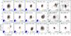 |
Fig. 2 Moment 0 maps of molecular emission toward W3 IRS5. The 353.6-GHz continuum emission is also presented for comparison. In panels a) to l), the compact dataset is imaged using natural weighting, resulting in a resolution of |
3.2. Line emission
3.2.1. Molecular distribution
Within the passbands (342.6–344.6 GHz and 352.6–354.6 GHz), we identify 17 spectral features from 11 molecules (Table 2). Most emission features come from sulfur-bearing molecules such as CS, SO, 33SO, SO2, 33SO2, 34SO2 and H2CS. Others come from HCN, HC15N, HNCO and CH3OH. This set of lines covers upper level energies from 43 K to 1067 K and high critical densities (107–108 cm-3). Figure 2 shows a sample of molecular emission images toward W3 IRS5 using the compact-configuration data and natural weighting (panels (a) to (l), with a resolution of  , PA − 12°) and with uniform weighting (panels (m) to (r), with a resolution of
  , PA − 17°).
Most of the emission from SO and SO2 and their isotopologues peaks toward the continuum peaks SMM1 and SMM2, while weaker emission is seen toward SMM3 and SMM4. However, other sulfur-bearing molecules such as CS and H2CS show a very different spatial distribution, and mainly peak to the north-west of SMM1–5 (Figs. 2i and m). Most of the emission from HCN and its isotopologues comes from SMM1 and SMM2 (Figs. 2g, h and n). Additional emission can be seen toward SMM3 and SMM4, as well as east and north-west of the SMM sources. The typical hot-core molecule CH3OH exclusively peaks toward SMM3 and SMM4 (Fig. 2k). HNCO is detected toward SMM1 and SMM2 only (Fig. 2j). Combining all these observational facts, the overall molecular emission toward W3 IRS5 can be classified into four zones (A: SMM1/SMM2; B: SMM3/SMM4; C :north-west region; may be associated with SMM5; and D: east of SMM1–5), and summarized in Fig. 3.
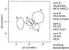 |
Fig. 3 Main molecular zones identified toward W3 IRS5. The representative molecular species including their isotopologues are listed. The crosses, filled circles and open squares represent the same sources as in Fig. 2. |
3.2.2. Velocity channel maps
Among the detected spectral features, most of the emission is compact (in zones A and B). Only CS J = 7–6, SO NJ = 88–77 and HCN J = 4–3 are extended and trace the large scale gas kinematics. Figure 4 shows the channel maps of these molecules from − 49 km s-1 to − 30 km s-1 and from − 41 km s-1 to − 35 km s-1, using robust weighting (robust = 0). These three molecules show emission over a broad velocity range. The emission at extreme velocities is mainly concentrated toward zone A. Weaker emission is seen toward zone B. Zone C is best traced by CS with some emission from SO, HCN, and H2CS as well. At velocities ranging from − 49 to − 42 km s-1, the emission from all three molecules can be seen toward zone D.
Of these three molecules, the image quality near the systemic velocity (~− 39.0 km s-1) is poor due to the missing flux of extended emission. However, some additional emission features can be seen near the systemic velocity. Figure 4 shows the channel maps of CS, SO and HCN at velocities ranging from − 41 km s-1 to − 35 km s-1. The emission of HCN is much weaker than the other species near − 39 km s-1 suggesting that HCN is much more extended, and therefore more heavily filtered out by the interferometer, or that the emission is self-absorbed. Additional extended emission in the N–S and NW–SE directions can be seen in the CS channel maps from − 41 km s-1 to − 38 km s-1, which might delineate two collimated outflows or a single wide-angle outflow in the NW–SE direction. The small velocity range suggests that the outflow may be in the plane of sky. In the SO channel maps, a bar-like structure can be seen from − 41 km s-1 to − 37 km s-1. Our data suggest that CS, SO and HCN trace different parts of the molecular condensation in W3 IRS5 and show a complex morphology in velocity space.
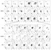 |
Fig. 4 Velocity channel maps of CS J = 7–6, SO NJ = 88–77 and HCN J = 4–3 toward W3 IRS5. Robust weighting (robust = 0) is used for the imaging, resulting resolutions of |


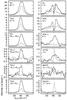 |
Fig. 5 Hanning-smoothed molecular spectra toward molecular zone A (thick line; offset position (− 0.42″, − 0.43″)) and B (thin line; offset position (− 1.89″, − 1.78″)). The compact-configuration dataset and natural weighting is used for all molecules except CS 7–6, SO NJ = 88–77 and HCN 4–3 which are taken from the combined dataset using natural weighting but convolved to the beam size of the compact dataset ( |
3.2.3. Line profiles
Figure 5 presents the hanning-smoothed spectra toward zone A (thick line; offset position − 0.42″, − 0.43″) and B (thin line; offset position − 1.89″, − 1.78″) where most of the detected molecules peak. The compact-configuration dataset and natural weighting is used for all molecules except CS, SO and HCN, which are imaged with the combined dataset in natural weighting and convolved to the same resolution as the other images.
SO shows a flat-top line profile at both positions, implying the line may be optically thick or is a blend of multiple velocity components. If SO is fully thermalized, optically thick, and fills the beam, the peak brightness temperatures indicate kinetic temperatures of ~70 K and ~45 K for zone A and B, respectively. These values are lower limits to the kinetic temperature if the beam filling factor is not unity. In addition, a blue-shifted spectral feature is seen at zone B.
CS and HCN show broad line profiles with a dip near the systemic velocity due to missing flux of extended emission. Single-dish JCMT observations of the same transitions (Helmich & van Dishoeck 1997) show single-peaked profiles and rule out self absorption. The line profiles at zone A are comparable with more emission in the blue-shifted line wing, suggesting both species trace similar cloud components. At zone B, both lines also show broad line wings. Near systemic velocity, HCN shows a wider dip than CS, suggesting that the spatial distributions of both lines are different. Vibrationally excited HCN peaks mainly toward zone A and shows an asymmetric line profile. HC15N is present toward both zones; its smaller line width toward zone B implying that this zone is more quiescent than zone A.
The line profiles of all the other molecules presented in Fig. 5 are Gaussian toward both zones. There is no significant velocity shift between the two zones. We note that the apparent velocity shift seen in 33SO and 33SO2 is due to the blending of multiple hyperfine transitions; we have defined the velocity axis with respect to the hyperfine component with the lowest frequency (Table 2).
We derive the line center LSR velocity (VLSR), FWHM line width (dV) and integrated line intensity (W) of the line profiles in zones A and B using Gaussian decomposition (Table 3). Since the CS and HCN line profiles are highly non-Gaussian, we do not attempt to derive the line parameters. For molecules with hyperfine transitions such as 33SO, 33SO2 and HNCO, we assume that each component has the same FWHM line width and LSR velocity. The relative intensity of hyperfine components are calculated assuming LTE and we fit the combined profile to the data. The results are summarized in Table 3. From the Gaussian fit, we do not find significant differences in LSR velocity between zones A and B. Different line widths are derived in both zones depending on the molecular transitions but the general trend is that the lines are broader in zone A, suggesting a more turbulent environment.
We estimate the amount of missing flux of CS 7–6, SO 88–77, HCN 4–3, and 32SO2 343,31–342,32 by comparing our SMA observations with the JCMT observations (Helmich & van Dishoeck 1997). Our SMA observations miss ~70%, ~40%, and ~80% flux for CS, SO, and HCN, respectively. Given the excitation of these lines, the derived missing flux is consistent with the large amount missing flux at 850 μm (~94%; Sect. 3.1). The SMA observation of 32SO2 343,31–342,32 likely recovers all emission, because this transition has a high upper level energy (corresponding to 582 K), and the emission therefore preferentially traces the dense, warm, and compact part of W3 IRS5.
4. Analysis
4.1. Mass and density of the submillimeter sources
We estimate the H2 column density and mass of each point source based on the continuum at 353.6 GHz. The H2 column density at the emission peak can be estimated as 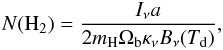 (1)where Iν is the peak flux density, a is the gas-to-dust ratio (100), Ωb is the beam solid angle, mH is the mass of atomic hydrogen, κν is the dust opacity per unit mass and Bν(Td) is the Planck function at dust temperature Td. We apply the interpolated value of κν(845μm) ≈ 2.2 cm2 g-1 as suggested by Ossenkopf & Henning (1994) for gas densities of 106–108 cm-3 and coagulated dust particles with thin ice mantles. The dust temperature of all five submillimeter sources is assumed to be 150 K (see excitation analysis, Sect. 4.2). The gas mass for each continuum peak is estimated from the total flux derived from the visibility fit (Table 1) via
 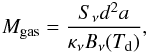 (2)where Sν is the total flux density of dust emission and d (1.83 kpc) is the distance to the source. Assuming a spherical source with 1″ in size, the H2 number density is also derived. We summarized the results in Table 1.
Gaussian decomposition of the line profiles in W3 IRS5.
From the density and mass estimates, we find beam-averaged H2 column densities, masses and volume densities toward SMM1, and SMM2 of about 3–4 × 1023 cm-2, 0.5 M⊙ and 3 × 107 cm-3, respectively. Toward SMM3, SMM4, and SMM5 values lower by factors 2–3 are found. The derived H2 column densities and masses are sensitive to the adopted dust opacity and temperature. If a bare grain model is adopted (Ossenkopf & Henning 1994), the derived values are reduced by a factor of <3. For dust temperatures between 100 and 200 K, the derived values change by a few ten% only. If the dust temperature is 30 K, the reported H2 column densities and masses increase by factors of ~5. The excitation analysis of Sects. 4.2.1 and 4.2.2 suggest such low temperatures are unlikely. The estimated H2 volume density is sensitive to the assumed source size as size-3. For example, the densities toward SMM1 and SMM2 increase to 2.4 × 108 cm-3 if the source size decreases to  . Since the submillimeter continuum peaks are unresolved, we treat the H2 volume densities of Table 1 as lower limit. We note that the core masses are all small (<1 M⊙).
4.2. Excitation analysis: temperatures
The detected molecular transitions, covering Eu from 43 K to 1067 K and critical densities of ~107–108 cm-3 (Table 2), form an useful dataset for the diagnostics of the physical conditions toward W3 IRS5. Among these molecular lines, multiple detections of the transitions from SO2 and 34SO2 toward zones A and B allow us to perform excitation analysis. Multiple detections of CH3CN J = 12–11 transitions reported by Wang et al. (2012) form another useful dataset for additional constraints of the excitation conditions toward zone B. We describe the details in the following two sections.
4.2.1. Rotational diagram
The molecular excitation conditions can be estimated via rotation diagram analysis assuming all the transitions are optically thin and the emission fills the beam. In a rotation diagram, the column density of the upper state Nu is given by  (3)where gu is the total degeneracy of the upper state, Ntot is the total molecular column density, Q is the partition function, Eu is the upper level energy, k is the Boltzmann constant and Trot is the rotational temperature. The left-hand side of Eq. (3) can be derived from the observations via
  (4)where θa and θb are the major and minor axes of the clean beam in arcsec, respectively, W is the integrated intensity in Jy beam-1 km s-1, gI and gK are the spin and projected rotational degeneracies, respectively, ν0 is the rest frequency in GHz, S is the line strength and μ0 is the dipole moment of the transition in Debye. Figure 6 plots the logarithm of the column densities from our data (Eq. (4)) versus Eu/k (Eq. (3)) and a fitted straight line with Trot and Ntot as free parameters. We adopt a 20% uncertainty of the integrated intensity in the analysis.
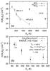 |
Fig. 6 a) Rotation diagram of SO2 (filled squares) and 34SO2 (filled triangles) toward zone A. The straight lines are the model fit. The derived rotational temperatures are indicated. b) Rotation diagram of CH3CN J = 12–11 toward zone B (open circles) taken from Wang et al. (2012). The best-fit model from the RADEX LVG analysis is overplotted for comparison (filled symbols). |
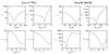 |
Fig. 7 RADEX excitation analysis toward zone A traced by 34SO2 (left four panels) and zone B traced by CH3CN (right four panels). The χ2 surfaces near the best-fit solution on each parameter axis are displayed. |
Figure 6a shows the rotation diagrams of SO2 and 34SO2 toward zone A, which sample level energies from 88 K to 1038 K (Table 2). 34SO2 is detected in five transitions with Eu ranging from 88 to 580 K, and indicates a Trot of 141 ± 25 K. However, the curvature in the distribution of the points implies that there might be a cooler and a warmer component along the line of sight. A two-component fit to the data gives Trot = 89 ± 10 K and Trot = 197 ± 55 K. The gas component traced by SO2 (Eu = 582 and 1038 K) implies a rotational temperature of 233 K, compatible with the temperature of the warm component derived from 34SO2 but obviously less well constrained because only two data points are available.
Molecular excitations in W3 IRS5.
The curvature in the 34SO2 rotation diagram (Fig. 6a) may also be due to line opacity (unlikely for the 34SO2 isotopologue) or subthermal excitation (see next section). The relatively abundant main-isotope SO2 may have optically thick lines, leading to an overestimate for Trot. However, we detected the 343,31 − 342,32 transition of both SO2 and 34SO2. Equation (4) yields a Nu(SO2)/Nu(34SO2) ratio of ~20 at 50 − 300 K, consistent with the 32S/34S ratio of 22 in the interstellar medium (Wilson & Rood 1994), suggesting that the 343,31 − 342,32 transition of SO2 (and its isotopologues) is optically thin. The 242,22 − 233,21v2 = 1 transition of SO2 is also likely optically thin since its Einstein-A coefficient is only about a factor of 2 greater than that of the 343,31 − 342,32 transition. These considerations suggest the a temperature gradient in zone A explains the rotation diagrams, with a cooler region at ~100 K and a warmer region of ≥200 K (Table 4).
We do not have enough data to obtain a reliable temperature estimate toward zone B (Table 3). Only the lowest two transitions of 34SO2 in level energy are detected here, and imply a rotational temperature of about 133 K. To have a better constraint of the excitation conditions toward zone B, we took the CH3CN J = 12 − 11 lines obtained by Wang et al. (2012) with the SMA at a resolution of 4.0″ × 2.6″. This molecule peaks toward zone B exclusively and shows a much narrower FWHM line width (~1.6 km s-1) compared to 34SO2 (~4 km s-1), suggesting a different molecular condensation in zone B. Figure 6b shows the CH3CN J = 12 − 11 K = 0 − 4 rotation diagram. The scatter in the data indicates that the lines are not optically thin. Therefore, we cannot carry out rotation diagram analysis on the CH3CN lines, and instead perform an LVG analysis in Sect. 4.2.2.
4.2.2. RADEX LVG model
To further investigate the physical conditions such as kinetic temperature (Tkin), column density (Ntot) and H2 volume density (nH2) toward zone A and B, we performed statistical equilibrium calculations to solve the level populations inferred from the observations. The purpose here is to have a crude estimate. Detailed analysis of temperature and density profiles in W3 IRS5 is beyond the scope of this work. We used the code RADEX (van der Tak et al. 2007) which solves the level populations with an escape probability method in the large-velocity-gradient (LVG) regime. Limited by the available observed data and collisional rate coefficients (Schöier et al. 2005), we perform calculations only for the 34SO2 lines and CH3CN J = 12 − 11 lines (Wang et al. 2012). For 34SO2, we adopted the collisional rate coefficients from SO2 (Green 1995)6 as an approximation since both species have similar molecular properties. The collisional rate coefficients of CH3CN are taken from Green (1986). To find the best-fit solution, we applied χ2 minimization to the 4-dimensional parameter space (Tkin, Ntot, nH2 and f, the beam filling factor).
Figure 7 shows the χ2 surfaces near the best-fit solution on each parameter axis, and Table 4 summarizes the results. Toward zone A, we use four 34SO2 lines (excluding the transition with Eu = 580 K) in the calculations due to the limited table of collisional rate coefficients. The RADEX calculations suggest that the kinetic temperature traced by the 34SO2 lines is about 90 K, consistent with the temperature derived from rotation diagram analysis and suggesting the excitation is thermalized. This requires a high H2 volume density (>109 − 10 cm-3) toward zone A. Apparently, the cool component toward zone A is very dense. Toward zone B, our RADEX calculations indicate a kinetic temperature of 160 K. Interestingly, the H2 volume density traced by CH3CN is only about 105 cm-3, lower than the critical density of a few 106 cm-3, implying subthermal excitation. The beam filling factor is about 0.8. The best-fit model for CH3CN is plotted as filled squares in Fig. 6b.
Alternatively, the excitation conditions toward zone A and B can be estimated via the line ratio of the 191,19 − 180,18 over the 104,6 − 103,7 transition of 34SO2 of 1.8. We assume that both transitions have the same filling factor. Using a FWHM line width of 5.0 km s-1 (the average FWHM line widths in zones A and B are 6.0 km s-1 and 4.0 km s-1, respectively) in the RADEX calculations, we calculate the intensity ratio as function of Tkin and Ntot for four different values of nH2 (Fig. 8). We again assume that the two transitions in the RADEX calculations have the same filling factor. These calculations suggest a high density of >109 cm-3 traced by 34SO2 toward zone A and B. The kinetic temperatures are ≥150 K, depending on the H2 volume density.
Combining the results from the rotation diagram analysis and the RADEX LVG calculations, we conclude that the gas traced by 34SO2 is dense (nH2 ≥ 109 cm-3) in zones A and B. There is a temperature gradient along the line of sight in zone A, characterized by a cool region of ~100 K and a warm region of ≥200 K. Toward zone B, the temperature gradient is less prominent. However, a quiescent (FWHM line width 1.6 km s-1) and less dense region (nH2 ~ 105 cm-3) traced by CH3CN is also present in zone B.
4.2.3. Molecular column density
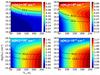 |
Fig. 8 RADEX analysis of the 34SO2 line ratios toward zone A and B assuming a FWHM line width 5.0 km s-1. The intensity ratios 191,19 − 180,18/104,6 − 103,7 are plotted in color scale. The observed integrated intensities of the 191,19 − 180,18 transition are plotted in curves (zone A: ~63 Jy beam-1 km s-1, zone B: ~15 Jy beam-1 km s-1). Toward both zones, the line ratio is about 1.8 (Table 3). Our results suggest that a high H2 volume density (> 109 cm-3) is needed to reproduce the observed line ratios. |
We estimate the beam averaged () molecular column density of each detected molecule toward zone A and B via Eq. (5) by assuming optically thin emission and a single rotational temperature of 150 K which is a representative value in W3 IRS5 (see previous two sections).  (5)We only use the ground vibrational state for the estimates. If multiple transitions of a given molecule are detected, we adopt the averaged value. The uncertainty of the exact rotational temperature results in an error in the column density of a few 10% (for Trot from 100 K to 200 K). As a consistency check, we estimate the line center opacity of each transition via
  (6)where c is the speed of light, Aul the Einstein-A coefficient, and ΔV the FWHM line width. All lines are consistent with the optically thin assumption (τ ≪ 1); only SO has line center opacities as large as τ ~ 0.3–0.5). Therefore, a lower limit of SO column density is derived.
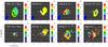 |
Fig. 9 First moment maps of different molecules observed toward W3 IRS5. The upper four maps are derived from the compact-configuration dataset with natural weighting, while the bottom four maps are made from the combined dataset using uniform weighting. The markers are identical to the ones in Fig. 1. The zero position is the phase center. We note that the velocity ranges are the same for all maps except HCN 4–3. |
A more representative value for SO can be derived from 33SO by assuming the isotopic ratio 32S/33S of ~132 (Wilson & Rood 1994; Chin et al. 1996). To convert the molecular column densities into fractional abundances with respect to H2, we adopt H2 column densities of 1.5 × 1023 cm-2 and 8.9 × 1022 cm-2 toward zone A and B, respectively (derived from the continuum image in Fig. 2l with the same assumptions described in Sect. 4.1). We summarize the results in Table 4. Toward zone A and zone B, SO and SO2 are very abundant with fractional abundances up to few 10-6, several orders of magnitude higher than found in dark clouds (few 10-9, Ohishi et al. 1992). This is indicative of active sulfur chemistry. Among the detected molecules, we do not see significant differences in fractional abundance between zones A and B, except for CH3OH which is a factor of 10 more abundant in zone B.
4.3. Kinematics
Complex velocity fields in W3 IRS5 are observed in various molecules. Figure 9 shows several first moment maps derived from different molecules. The upper four maps are made from the compact-configuration dataset using natural weighting, while the bottom ones are derived from the combined dataset with uniform weighting. Different velocity gradients are observed in 34SO2 (NW–SE), HC15N (E–W) and HCN v2 = 1 (NE–SW). CH3OH shows an interesting velocity distribution with a slightly blue-shifted emission peak (SMM3 and SMM4). Comparing the velocities near SMM3 and SMM4 derived from 34SO2 and CH3OH, we suggest that there are two distinct regions along the line of sight. Indeed, the line widths of these two molecules are very different (Table 3). At one-arcsecond resolution (combined dataset with uniform weighting), 34SO2 peaks toward SMM1 and SMM2, and shows a velocity gradient consistent with the NW–SE gradient found from lower angular resolution observations. For the three strongest lines, CS, SO and HCN, we adopted uniform weighting to form the images in order to minimize the strong sidelobes which otherwise corrupt the images. CS and HC15N show similar velocity patterns with some patchy velocity shifts. The velocity field traced by SO is very different from the ones seen from other molecules in Fig. 9, which is likely due to opacity effects. Near SMM1 and SMM2, HCN and its vibrationally excited transition show similar velocity patterns. The velocity components traced by CS and HCN toward zone C are red-shifted with respect to the systemic velocity (~− 39 km s-1). However, a clear velocity jump is seen near SMM5 if we compare the maps of 34SO2 to CS and HCN, implying that the gas component in zone C is not closely related to the ones in zones A and B. Another velocity jump is seen in the HCN map if we compare the velocities in zones A and D, suggesting that the gas component in zone D is also not closely related to zones A and B.
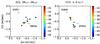 |
Fig. 10 Channel-by-channel locations of the emission peaks of the SO2 343,31 − 342,32 and HCN 4–3 v2 = 1. The emission peaks are color-coded with respect to their VLSR in km s-1 shown in the color wedge. Two distinct, orthogonal velocity gradients are seen. |
In Fig. 9, we see that the velocity gradients seen in 34SO2 and HCN v2 = 1 are roughly perpendicular to each other. To confirm this, we fit the emission of HCN 4–3 v2 = 1 (Eu = 1067 K) and SO2 343,31 − 342,32 (Eu = 582 K) (compact configuration with natural weighting) channel-by-channel with a Gaussians to determine the movement of the peak positions. In Fig. 10, the velocity gradient seen in SO2 is roughly perpendicular to the line joining SMM1 and SMM2, while the velocity gradient observed in the vibrationally excited HCN is parallel to this line. The vibrationally excited HCN may trace outflow or jet emission since the observed velocity gradient is parallel to the free-free emission knots observed by Wilson et al. (2003). We suggest that SO2 traces a rotating structure orthogonal to this outflow axis.
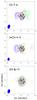 |
Fig. 11 Integrated intensity maps at different velocity ranges (blue: −50 to −43 km s-1; green: −43 to −35 km s-1; red: −35 to −28 km s-1). We adopted the combined-configuration dataset in natural weighting in order to show the additional weak emission features. The contour levels of each Doppler-shifted component for CS, HCN and SO are 15, 20, 30, 40,...%, 10, 20, 30,...% and 5, 10, 20, 30,...% of the emission peak, respectively. We note that the first contours are all ≥3σ noise level. The markers are identical to the ones in Fig. 1. |
In our data, only the CS 7–6, HCN 4 − 3 and SO NJ = 88 − 77 emission show a wide velocity range (about 30–40 km s-1; Fig. 5), presumably due to outflow activity in W3 IRS5. To study the distribution of the high velocity components (Fig. 11), we integrate the emission over three different velocity ranges (blue: −50 to −43 km s-1, green: −43 to −35 km s-1 and red: −35 to −28 km s-1). We took the combined-configuration dataset and used natural weighting for the analysis. The images are plotted with contours starting well above 3σ to minimize the impact of sidelobes, especially for the green component. As seen in Fig. 11, the high-velocity components of all three molecules peak near zone A and close to SMM2, suggesting a bipolar outflow with an inclination close to the line of sight. The existence of a line-of-sight outflow also implies a rotating structure in the plane of the sky, in which SMM1 and SMM2 form a binary system. Therefore, the small scale velocity gradients (Fig. 10) seen in HCN 4–3 v2 = 1 and SO2 may highlight the kinematics of the envelope. Additional blue-shifted components are seen toward zone D. The green component of CS highlights the gas in zone C. In the HCN map, the emission in zone D together with the emission peaking near the offset position (− 8″, 0″) may form another bipolar outflow in the E–W direction since the line connecting these peaks passes through zone A which contains star-forming cores. In this case, the one-arcsecond scale velocity gradients seen in Fig. 10 imply a complex motion (rotation plus expansion or contraction) in the common envelope of SMM1 and SMM2. To summarize, the kinematics in W3 IRS5 is very complex and requires additional observations at high resolution with good image fidelity for further analysis.
5. Discussion
5.1. Star formation in W3 IRS5
5.1.1. Different evolutionary stages within W3 IRS5
Based on the continuum image at 353.6 GHz, we identified five compact sources (SMM1 to SMM5) toward W3 IRS5 (Fig. 1 and Table 1). SMM1 and SMM2 also show compact cm-wave emission (Wilson et al. 2003; van der Tak et al. 2005) indicating that stars sufficiently massive to ionize their surroundings have formed (>8 M⊙). The non-detection of compact cm-wave emission toward SMM3, SMM4 and SMM5 implies that currently those cores have not (yet) formed massive stars. By comparing the 353.6-GHz continuum with the NICMOS 2.22 μm emission and cm-wave emission (Fig. 1a, Megeath et al. 2005; Wilson et al. 2003; van der Tak et al. 2005), we suggest that the eastern part (SMM1 and SMM2) of the source is more evolved than the western part (SMM3, SMM4 and SMM5). The small core mass (~0.3 M⊙) suggests that SMM3–5 may be forming low-mass stars or are starless cores.
For a virialized star-forming core (Mcore + Mstar ≈ Mvir), the 1D virial velocity dispersion (σvir; cf. McKee & Ostriker 2007) is  (7)where r is the radius of the source, G is the gravitational constant, and Mvir is the virial mass. Assuming a core radius of 0.5″, core gas masses of ~0.3 M⊙, and stellar masses of SMM3–5 less than 8 M⊙, the 1D virial velocity dispersions should be no more than 1.3 km s-1. From our observations of CH3OH line toward SMM3/4 and CS line toward SMM5, the inferred 1D velocity dispersions (σ = ΔV/
 ) are 1.0 km s-1 and 1.4 km s-1. The large observed line widths suggest that either these cores contain stars just under 8 solar masses, or the clumps may have smaller mass stars, and the large velocities may be the influence of outflows from SMM1/2. In the latter, case, it is not clear if the gas in the cores is gravitationally bound. Subarcsecond observations of dust continuum and outflow tracers should tell if SMM3–5 are low-mass starless leftover cores after the formation of SMM1–2 or harbor low-mass protostars under the influence of outflows from SMM1–2.
5.1.2. Fragmentation and Jeans analysis
From the continuum analysis, we found the core masses of the identified SMM sources are small (0.2–0.6 M⊙) and the projected distance between the SMM sources are about 1″ − 2″ (1800–3600 AU). This observed structure, in the meantime, is still embedded in a large massive core with size about 1′ and mass of several hundred M⊙ (W3-SMS1 in the SCUBA 850 μm image, Di Francesco et al. 2008; Wang et al. 2012). At 1′ scale, Megeath et al. (1996) found that there are ~300 low-mass stars in the core surrounding W3 IRS5 with a stellar density of few 1000 pc-3. Therefore, it is interesting to investigate the cloud structure from 1′ scale to 1″ to see what determines the overall core/stellar mass distribution and their spatial distribution. To study this question, we perform Jeans analysis in W3 IRS5 based on our SMA continuum image and the JCMT SCUBA 850 μm image (Di Francesco et al. 2008; Wang et al. 2012). The Jeans length and Jeans mass are expressed as (cf. Stahler & Palla 2005, Eqs. (9.23) and (9.24)): 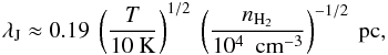 (8)and
 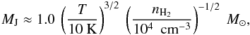 (9)where T is the kinetic temperature and nH2 is the H2 volume density. These two quantities are more sensitive to the adopted H2 volume density. To estimate the 1′ scale H2 density, we measured the total flux density in a 1′ by 1′ box centered toward W3 IRS5 using the SCUBA 850 μm image. Using the same prescription outlined in Sect. 4.1, a total flux density of 160 Jy corresponds to a mass of 950 M⊙ assuming a dust temperature of 40 K. The mean H2 volume density is 2.4 × 105 cm-3. Therefore, at 1′ we derived the Jeans length and Jeans mass to be 16 000 AU (~9′′) and 2 M⊙, respectively. Interestingly, these two characteristic quantities seem to match the observed spatial separations of low-mass stars (18 000–12 000 AU, Megeath et al. 1996), implying that the spacing of the young low mass stars are consistent with gravitational fragmentation. The Jeans masses are greater than the mean stellar mass for a standard initial mass function (0.5 M⊙), which is expected given a typical efficiency of low-mass star formation ~30% (Alves et al. 2007). Toward the central regions of W3 IRS5, the temperature (~140 K) and density (few 107 cm-3) are higher than the values on the scale of the entire core. The corresponding Jeans length and Jeans mass are 2700–3800 AU (1.5″–2.1″) and ~1 M⊙, respectively. The Jeans length is consistent with the observed spacing of the SMM cores, implying that gravitational fragmentation may be occurring in the dense, warm center of the cluster. On the other hands, the implied Jeans masses are much smaller. This immediately leads to the question how the massive stars in SMM1/2 accreted their current masses.
5.1.3. Accretion rates
The largest accretion rate that an object can sustain is essentially given by its mass divided by its free-fall time, 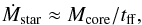 (10)where
  and
and  is the mean density. The masses of the SMM1–5 cores come from Table 1. We use the observed size for the SMM1–5 cores, which are set to 1″ in diameter based on Fig. 1a. We adopt stellar masses of 20 M⊙ for SMM1 and SMM2 based on the total luminosity of 2 × 10⁵L⊙. We use the combined stellar and core masses and the core radii to determine the average baryonic density; the corresponding free-fall times are ~1000 yr for SMM1/2, and >1700 yr for SMM3–5. These imply mass accretion rates of 5 × 10⁻⁴M⊙ yr-1 for SMM1/2, and < 2 × 10⁻⁴M⊙ yr-1 for SMM3–5. The upper limits for the latter follow from the upper limit on the embedded stellar masses of 8 M⊙. The accretion rates are consistent with those expected for the formation of massive stars (Keto 2003). The combination of small core masses and high accretion rates imply very short time scales of a few thousand years. If the massive stars in SMM1/2 form from accretion of the local cores (1″ scales), the low core masses imply that they are now in a stage that most of core mass has been accrete onto the stellar components. On the other hand, the SMM cores may be accreting material that have been resolved out by the interferometers on scales >1″. In this case, the reservoir of material from which the cores are accreting is larger than the observed projected spacing of the protostars, implying that the accretion is coming from a global collapse of the molecular core in which the proto-Trapezium is embedded.
To determine whether it is possible that the massive stars in W3 IRS5 are being fed from the collapse of the surrounding core, we estimate the potential accretion rates from this accretion. The free-fall time for the central 1′ W3–SMS1 condensation, with a total mass of 950 M⊙ and an embedded stellar mass of ≲50 M⊙, is 72 000 yr and the free-fall mass accretion rate is 1 × 10⁻²M⊙ yr-1. We note that the derived accretion rate is the maximum rate of infall assuming free-fall collapse. In the central region, the amount of gas accreted by each star is given by 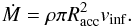 (11)(Bonnell et al. 2001), where vinf is the infall gas velocity, ρ is the density of the gas surrounding the proto-Trapezium, and Racc is the radius within which the infalling gas is accreted onto a specific star. We assume nH2 = 106 cm-3 to compute ρ, which is intermediate between the density of the surrounding 1′ diameter core (105 cm-3) and the core of the inner 1″ (107 cm-3). Given FWHM line widths of 2–5 km s-1, we adopt a vinf equal to the 3D gas velocity dispersion implied by the FWHM line width (
 ), which is 1.5–3.7 km s-1 with a mean value of 2.6 km s-1. The uncertainty of vinf gives a factor of <3 in error of accretion rate. The possible values for Racc are the radius set by the motions of the stars through the gas (Bondi-Hoyle radius) and the radius set by tidal interaction of the stars with the gravitational potential of the cluster core (tidal radius). The actual accretion rate is given by the minimum of these two radii (Bonnell et al. 2001). To estimate Racc due to tidal interactions, we use the equation from Bonnell et al. (2001) and rewrite in terms of the gas density around the star,
  (12)In this case,
  are 4700 AU and 3500 AU for a 20 M⊙ and 8 M⊙ central star embedded in a core with gas density 106 cm-3, respectively. The accretion rates are then 2 × 10⁻⁴M⊙ yr-1 and 1 × 10⁻⁴M⊙ yr-1 for the 20 M⊙ and 8 M⊙ stars, respectively. Alternatively, the motions of the stars through the cloud can limit the gas accretion; only the gas within a radius where the escape velocity is less than the velocity of the star relative to the gas can be accreted. The Racc in this case can be approximated by the Bondi-Hoyle radius:
  (13)The resulting
  are 5200 AU and 2100 AU for the 20 and 8 M⊙ stars, and the mass infall rates are 3 × 10⁻⁴ M⊙ yr-1 for a stellar mass of 20 M⊙ and 4 × 10⁻⁵M⊙ yr-1 for a stellar mass of 8 M⊙.
As a result, from our basic analysis, global collapse of the core and subsequent accrete of the material from the collapse onto the stars can sustain infall rates in excess of 10-4 M⊙ yr-1 for SMM1/2 and are sufficient to sustain high mass star formation. For SMM3–5, the rates are 10 times lower. However, the local density around SMM3–5 is closer to 107 cm-3, the actual densities and the accretion rates may be higher. The fact that the stellar accretion rates is two orders of magnitude less than the free-fall accretion rate for the large cores suggests that there is sufficient infall of material to feed the accretion of the individual stars, even if the actual collapse times is ten free fall times.
In summary, we find two alternatives. Either the massive stars accrete locally from their local cores; in this case the small core masses imply W3 IRS5 is at the very end stages (1000 yr) of infall and accretion. Alternatively, the stars are accreting from the global collapse of a massive, cluster forming core. This later scenario is similar to the competitive accretion models of massive star formation (e.g., Bonnell & Bate 2006). For the two massive objects SMM1/2, the observed densities and velocity widths are consistent with those needed for the global collapse to feed accretion onto the massive stars at rates of ~ 10-4 M⊙ yr-1. For the remaining objects, SMM 3–5, a lower infall rate is estimated; perhaps these are forming intermediate mass stars, although the rate of accretion may rise as they increase in mass as precede by the models of competitive accretion. However, a clear detection of the infall of gas has not yet been observed. This makes the W3 IRS5 cluster a perfect region to further test the competitive accretion model, if the kinematics of the gas motions can be traced on scales from 1′ down to <1″. Future single-dish and interferometric observations of this region, e.g., combining SMA or PdBI observations with IRAM 30 m measurements, are required to fully map the gas flow across these scales.
5.2. The molecular environment of W3 IRS5
5.2.1. Distinct molecular zones
A JCMT spectral line survey characterized W3 IRS5 as a remarkable massive star-forming region with rich spectral features from sulfur-bearing molecules (Helmich et al. 1994; Helmich & van Dishoeck 1997). Helmich et al. (1994) also reported that the CH3OH abundance is remarkably low, even compared to typical dark clouds. From our SMA data, and the results from Wang et al. (2012), we find that sulfur-bearing molecules such as SO, SO2 and their isotopologues, strongly peak toward the submillimeter sources SMM1 and SMM2 (zone A) with extended emission toward SMM3, SMM4 and SMM5 (Fig. 2). This suggests that SMM1 and SMM2 are the driving center of the sulfur chemistry. Interestingly, typical hot-core molecules such as CH3OH (Fig. 2k) and CH3CN (Wang et al. 2012) peak toward SMM3/4 (zone B) exclusively, underlining the chemical differences between zones A and B. Moreover, toward zone B, there are two distinct regions along the line of sight with different physical characteristics. The narrow FWHM line widths seen in CH3OH (2.3 km s-1; Table 3) and CH3CN (1.6 km s-1; Wang et al. 2012) suggest that this “hot core” source is less turbulent compared to the gas component traced by SO and SO2, which have larger line widths (~4–7 km s-1; Table 3). As implied by the excitation analysis (Sect. 4.2.2), this “hot core” is less dense (~105 cm-3) than the gas traced by 34SO2 (≥109 cm-3). We suggest that this “hot core” may created by feedback from the star-forming activity associated with SMM1 and SMM2. It is, however, hard to tell if this core is heated internally or externally since we do not find significant temperature differences between 34SO2 and CH3CN (Sect. 4.2.2). In addition, there is another interesting chemical signature in W3 IRS5, where SO and SO2 are peaked toward zone A, while CS and H2CS are peaked toward zone C (Fig. 2). Although these species are chemically related (e.g. Charnley 1997), this spatial de-correlation implies that different chemical processes are involved, such as hot core versus shock chemistry (Hatchell & Viti 2002).
5.2.2. Abundances of SO, SO2 and CH3OH
It has been proposed that the abundance ratios of sulfur-bearing species can be used to measure the time elapsed since the start of ice-mantle evaporation in star-forming cores if proper physical conditions are applied (e.g. Charnley 1997; van der Tak et al. 2003; Wakelam et al. 2004). Unfortunately, the rough estimates of the SO and SO2 abundances provided by our data limit us to a qualitative comparison only. SO and SO2 are abundant toward W3 IRS5. The fractional abundance of SO and SO2 (Table 4) are, respectively, 8.6 × 10⁻⁶ and 9.4 × 10⁻⁷ toward zone A, and 5.4 × 10⁻⁶ and 2.8 × 10⁻⁷ toward zone B. This corresponds to SO2/SO ratios of 0.1 and 0.05 for zones A and B, respectively. The uncertainty of these ratios are factors of few, and SO2 is clearly less abundant than SO toward W3 IRS5.
Charnley (1997), Hatchell et al. (1998) and Wakelam et al. (2004) present chemical models that relate the SO2/SO ratio to the time since the onset of grain-mantle evaporation. Although these models are very sensitive to the initial mantle composition, cosmic ray ionization rate, density and temperature, these models show that the evolution of the fractional abundances of SO and SO2 peak after roughly 104–105 yr after grain-mantle evaporation. Such time scales are consistent with the free-fall time for the entire cluster calculated in Sect. 5.1.3 of (0.8–1.4) × 105 yr.
Toward the emission peak in zone B, we derive a CH3OH abundance of 5.1 × 10⁻⁸, lower by a factor of 10–100 compared to the abundance found toward the Orion Compact Ridge (Menten et al. 1988). This low CH3OH abundance implies that the “hot core” toward zone B is chemically young since large amounts of CH3OH are still observed in the solid state (Allamandola et al. 1992). Since zone B does show emission from SO and SO2, which is indicative of outflow activity (Fig. 11), it is possible that the “hot core” has just been turned on by external heating from zone A.
5.3. Non-detection of CO+: an indication of FUV origin
Just as much as detected emission can provide information, so can the non-detection of emission tell us something. Molecular ions and radicals like CN, NO, CO+, SO+ and SH+, are thought to trace high energy (far-ultraviolet, FUV, and X-ray) radiation toward star-forming regions (Sternberg & Dalgarno 1995; Maloney et al. 1996). Toward W3 IRS5, Stäuber et al. (2007) reported detection of two hyperfine transitions of CO+N = 3–2, F = 5/2–3/2 (353.7413 GHz) and F = 7/2–5/2 (354.0142 GHz) with the James Clerk Maxwell Telescope (JCMT) at 14″ resolution. They concluded that CO+ is present in FUV-irradiated cavity walls which may be part of the outflows along the line of sight, similar to AFGL 2591 (Stäuber et al. 2007; Benz et al. 2007; Bruderer et al. 2009). However, the detection of X-ray emission toward W3 IRS5 (Hofner et al. 2002) with a luminosity of ~ 5 × 1030 erg s-1 implies that CO+ may have an X-ray origin as well. The geometrical dilution of this X-ray flux down to the cosmic ray ionization level suggests that the source size of CO+ should be about 0.7″ if X-rays are the dominant source of CO+. Therefore interferometric observations would be helpful to determine if CO+ can have an X-ray origin.
The same set of CO+N = 3–2 hyperfine transitions are also covered in our SMA data. Emission at 353.7413 GHz is clearly detected toward zone A and shows a compact structure (cf. Fig. 2d). However, we do not detect the transition at 354.0142 GHz (Fig. 12). In LTE the intensity ratio of the CO+N = 3–2 hyperfine transitions (including F = 3/2–1/2 at 353.0589 MHz) is 1:14:20. A similarly compact source at 354.0142 GHz should therefore have been detected. Also, the CO+ abundance we derive from the 353.7413 GHz intensity (~1.3 × 10⁻⁹) is much larger than the prediction from Stäuber et al. (2007) and Stäuber & Bruderer (2009) (~ 10-12 − 10-10). We therefore rule out CO+ as the origin of the emission at 353.7413 GHz.
Instead, we assign the line near 353.741 GHz to 33SO2 194,16 − 193,17 transition, as was suggested by Stäuber et al. (2007). The anomalous CO+ line ratio reported by (Stäuber et al. 2007) is explained by blending of the CO+ line with 33SO2 at 353.741 GHz. If this assignment is correct, our SMA data should contain three other lines from 33SO2 (with hyperfine transitions), near 344.031 GHz (Eu = 397 K), 344.504 GHz (Eu = 232 K) and 354.246 GHz (Eu = 297 K). These lines are not detected, but they have either smaller line strengths (344.504 GHz) or decreased intensity due to hyperfine splitting (344.031, 354.246 GHz). In fact, the detected transitions near 353.741 GHz is expected to be the strongest in the passband. The assignment of this line to 33SO2 is further supported by the detection of its 111,11 − 100,10 line by Wang et al. (2012). From our data, we find a column density ratio of 32SO2/33SO2 of ~147 assuming optically thin lines and LTE conditions (Table 4). This ratio is consistent with the ISM 32S/33S ratio of ~132 (Wilson & Rood 1994; Chin et al. 1996).
The fact that CO+, detected in the JCMT beam, and undetected in our SMA data, suggests an extended (>21″) distribution of the emission consistent with an origin of the emission in the FUV-irradiated cavity walls, and rules out an X-ray origin. Alternatively, the non-detection of CO+ in our ~2.5″ beam may be explained if CO+ is destroyed rapidly with H2 or electrons (Stäuber & Bruderer 2009, and the references therein) in the high density (≥109 cm-3) material near SMM1 and SMM2 identified by our data.
 |
Fig. 12 Hanning-smoothed spectrum taken from the compact-configuration dataset toward zone A (offset position: − 0.42″, − 0.43″). The black lines are the observed data, while the red lines are the model spectrum of CO+N = 3–2, F = 3/2–1/2 (353.0589 GHz), 5/2–3/2 (353.7413 GMHz) and 7/2–5/2 (354.0142 GHz) under LTE assumption. The LTE intensity ratio of the hyperfine transitions is ~1:14:20 (increasing in frequency). The F = 7/2–5/2 transition at 354.0142 GHz is not detected in our SMA data. |
6. Conclusions
Our conclusions can be summarized as follows.
-
1.
The 1″ resolution continuum image at 353.6 GHz shows 5 compact submillimeter sources SMM1–5 (Fig. 1). SMM1 and SMM2 have embedded massive stars (~20 M⊙), judging from the detection of compact cm-wave emission. The other sources do not contain massive stars currently, and may be forming low-mass stars or simply be starless.
-
1.
The gas densities of SMM1–5 are high as 107 cm-3, but their core masses are surprizingly low, 0.2 − 0.6 M⊙.
-
2.
If the massive stars in W3 IRS5 accrete locally from the surrounding core, the derived small core masses of the SMM sources imply that the main accretion phase is almost concluded.
-
3.
From Jeans analysis, the cloud structures from 1′ scales down to 1″ scales are likely determined by gravitational fragmentation in turbulent environment.
-
4.
The free-fall accretion rates toward SMM1 and SMM2 are about 5 × 10⁻⁴ M⊙ yr-1, while SMM3–5 have accretion rates of less than 1–2 × 10⁻⁴M⊙ yr-1 if their stellar masses are 8 M⊙ or 2–4 × 10⁻⁵ M⊙ yr-1 if they are starless.
-
5.
If star formation in W3 IRS5 follows the competitive accretion model, global collapse of the core and subsequent accretion of the material from the collapse onto the stars can sustain infall rates in excess of 10-4M⊙ yr-1 for SMM1/2 and are sufficient to sustain high-mass star formation.
-
6.
From the molecular line images, we identified four molecular zones (Fig. 3). Zone A and B are the major places where sulfur chemistry and hot core chemistry are taking place. Zone C and D, however, seem kinematically unrelated to zone A and B. There is a “hot core” traced by CH3OH and CH3CN toward the line of sight of zone B.
-
7.
The large abundances of SO and SO2 with respect to H2 (few 10-7 to 10-6) derived in zone A and B are indicative of active sulfur chemistry.
-
8.
The low abundance of CH3OH (5 × 10⁻⁸) in the hot core toward zone B implies that it may be recently heated either internally or externally by feedback from zone A. Zone B seems chemically younger than zone A.
-
9.
The non-detection of CO+J = 3–2 on small scales supports the idea that CO+ is formed in the FUV-irradiated outflow cavity walls, and implies that X-rays either do not contribute significantly to the CO+ production or that this molecule is rapidly destroyed again in the dense material around SMM1 and SMM2.
The Submillimeter Array is a joint project between the Smithsonian Astrophysical Observatory and the Academia Sinica Institute of Astronomy and Astrophysics and is funded by the Smithsonian Institution and the Academia Sinica.
Recent calculations by Spielfiedel et al. (2009) and Cernicharo et al. (2011) show that the collisional rate coefficients calculated by Green (1995) are lower by a factor 3–5. The listed critical densities in Table 2 may be 3–5 times smaller.
Acknowledgments
We thank the anonymous referee and the editor Malcolm Walmsley for reviewing our paper. We also thank the SMA staff for conducting our observations. The research of K.-S.W. at Leiden Observatory is supported through a Ph.D. grant from the Nederlandse Onderzoekschool voor Astronomie (NOVA). This research has made use of NASA’s Astrophysics Data System Bibliographic Services.
References
- Abt, H. A., & Corbally, C. J. 2000, ApJ, 541, 841 [NASA ADS] [CrossRef] [Google Scholar]
- Allamandola, L. J., Sandford, S. A., Tielens, A. G. G. M., & Herbst, T. M. 1992, ApJ, 399, 134 [NASA ADS] [CrossRef] [PubMed] [Google Scholar]
- Alves, J., Lombardi, M., & Lada, C. J. 2007, A&A, 462, L17 [NASA ADS] [CrossRef] [EDP Sciences] [Google Scholar]
- Benz, A. O., Stäuber, P., Bourke, T. L., et al. 2007, A&A, 475, 549 [NASA ADS] [CrossRef] [EDP Sciences] [Google Scholar]
- Beuther, H., Churchwell, E. B., McKee, C. F., & Tan, J. C. 2007, Protostars and Planets V, 165 [Google Scholar]
- Bonnell, I. A., & Bate, M. R. 2006, MNRAS, 370, 488 [NASA ADS] [CrossRef] [Google Scholar]
- Bonnell, I. A., Bate, M. R., Clarke, C. J., & Pringle, J. E. 2001, MNRAS, 323, 785 [NASA ADS] [CrossRef] [Google Scholar]
- Bruderer, S., Benz, A. O., Doty, S. D., van Dishoeck, E. F., & Bourke, T. L. 2009, ApJ, 700, 872 [NASA ADS] [CrossRef] [Google Scholar]
- Campbell, M. F., Butner, H. M., Harvey, P. M., et al. 1995, ApJ, 454, 831 [NASA ADS] [CrossRef] [Google Scholar]
- Cernicharo, J., Spielfiedel, A., Balança, C., et al. 2011, A&A, 531, A103 [NASA ADS] [CrossRef] [EDP Sciences] [Google Scholar]
- Cesaroni, R., Felli, M., Testi, L., Walmsley, C. M., & Olmi, L. 1997, A&A, 325, 725 [NASA ADS] [Google Scholar]
- Charnley, S. B. 1997, ApJ, 481, 396 [NASA ADS] [CrossRef] [Google Scholar]
- Chin, Y.-N., Henkel, C., Whiteoak, J. B., Langer, N., & Churchwell, E. B. 1996, A&A, 305, 960 [NASA ADS] [Google Scholar]
- Claussen, M. J., Gaume, R. A., Johnston, K. J., & Wilson, T. L. 1994, ApJ, 424, L41 [NASA ADS] [CrossRef] [Google Scholar]
- Di Francesco, J., Johnstone, D., Kirk, H., MacKenzie, T., & Ledwosinska, E. 2008, ApJS, 175, 277 [NASA ADS] [CrossRef] [Google Scholar]
- Fontani, F., Caselli, P., Zhang, Q., et al. 2012, A&A, 541, A32 [NASA ADS] [CrossRef] [EDP Sciences] [Google Scholar]
- Gibb, A. G., Davis, C. J., & Moore, T. J. T. 2007, MNRAS, 382, 1213 [NASA ADS] [CrossRef] [Google Scholar]
- Green, S. 1986, ApJ, 309, 331 [NASA ADS] [CrossRef] [Google Scholar]
- Green, S. 1995, ApJS, 100, 213 [NASA ADS] [CrossRef] [Google Scholar]
- Hatchell, J., & Viti, S. 2002, A&A, 381, L33 [NASA ADS] [CrossRef] [EDP Sciences] [Google Scholar]
- Hatchell, J., Thompson, M. A., Millar, T. J., & MacDonald, G. H. 1998, A&A, 338, 713 [NASA ADS] [Google Scholar]
- Helmich, F. P., Jansen, D. J., de Graauw, T., Groesbeck, T. D., & van Dishoeck, E. F. 1994, A&A, 283, 626 [NASA ADS] [Google Scholar]
- Helmich, F. P., & van Dishoeck, E. F. 1997, A&AS, 124, 205 [NASA ADS] [CrossRef] [EDP Sciences] [Google Scholar]
- Ho, P. T. P., Moran, J. M., & Lo, K. Y. 2004, ApJ, 616, L1 [NASA ADS] [CrossRef] [Google Scholar]
- Hofner, P., Delgado, H., Whitney, B., Churchwell, E., & Linz, H. 2002, ApJ, 579, L95 [NASA ADS] [CrossRef] [Google Scholar]
- Imai, H., Kameya, O., Sasao, T., et al. 2000, ApJ, 538, 751 [NASA ADS] [CrossRef] [Google Scholar]
- Keto, E. 2003, ApJ, 599, 1196 [NASA ADS] [CrossRef] [Google Scholar]
- Krumholz, M. R., & Bonnell, I. A. 2009, Models for the formation of massive stars, ed. G. Chabrier (Cambridge University Press), 288 [Google Scholar]
- Longmore, S. N., Pillai, T., Keto, E., Zhang, Q., & Qiu, K. 2011, ApJ, 726, 97 [NASA ADS] [CrossRef] [Google Scholar]
- Maloney, P. R., Hollenbach, D. J., & Tielens, A. G. G. M. 1996, ApJ, 466, 561 [NASA ADS] [CrossRef] [Google Scholar]
- McKee, C. F., & Ostriker, E. C. 2007, ARA&A, 45, 565 [NASA ADS] [CrossRef] [Google Scholar]
- McKee, C. F., & Tan, J. C. 2003, ApJ, 585, 850 [NASA ADS] [CrossRef] [MathSciNet] [Google Scholar]
- Megeath, S. T., Herter, T., Beichman, C., et al. 1996, A&A, 307, 775 [NASA ADS] [Google Scholar]
- Megeath, S. T., Wilson, T. L., & Corbin, M. R. 2005, ApJ, 622, L141 [NASA ADS] [CrossRef] [Google Scholar]
- Megeath, S. T., Townsley, L. K., Oey, M. S., & Tieftrunk, A. R. 2008, Low and High Mass Star Formation in the W3, W4, and W5 Regions, ed. B. Reipurth, 264 [Google Scholar]
- Menten, K. M., Walmsley, C. M., Henkel, C., & Wilson, T. L. 1988, A&A, 198, 253 [NASA ADS] [Google Scholar]
- Mitchell, G. F., Hasegawa, T. I., & Schella, J. 1992, ApJ, 386, 604 [NASA ADS] [CrossRef] [Google Scholar]
- Müller, H. S. P., Schlöder, F., Stutzki, J., & Winnewisser, G. 2005, J. Mol. Struct., 742, 215 [NASA ADS] [CrossRef] [Google Scholar]
- Ohishi, M., Irvine, W. M., & Kaifu, N. 1992, in Astrochemistry of Cosmic Phenomena, ed. P. D. Singh (Dordrecht: Springer-Verlag) IAU Symp., 150, 171 [Google Scholar]
- Ossenkopf, V., & Henning, T. 1994, A&A, 291, 943 [NASA ADS] [Google Scholar]
- Peretto, N., André, P., & Belloche, A. 2006, A&A, 445, 979 [NASA ADS] [CrossRef] [EDP Sciences] [Google Scholar]
- Pickett, H. M., Poynter, R. L., Cohen, E. A., et al. 1998, J. Quant. Spec. Radiat. Transf., 60, 883 [Google Scholar]
- Pillai, T., Kauffmann, J., Wyrowski, F., et al. 2011, A&A, 530, A118 [NASA ADS] [CrossRef] [EDP Sciences] [Google Scholar]
- Pineau des Forets, G., Roueff, E., Schilke, P., & Flower, D. R. 1993, MNRAS, 262, 915 [NASA ADS] [CrossRef] [Google Scholar]
- Ridge, N. A., & Moore, T. J. T. 2001, A&A, 378, 495 [NASA ADS] [CrossRef] [EDP Sciences] [Google Scholar]
- Rodón, J. A., Beuther, H., Megeath, S. T., & van der Tak, F. F. S. 2008, A&A, 490, 213 [NASA ADS] [CrossRef] [EDP Sciences] [Google Scholar]
- Sault, R. J., Teuben, P. J., & Wright, M. C. H. 1995, in Astronomical Data Analysis Software and Systems IV, eds. R. A. Shaw, H. E. Payne, & J. J. E. Hayes, ASP Conf. Ser., 77, 433 [Google Scholar]
- Schöier, F. L., van der Tak, F. F. S., van Dishoeck, E. F., & Black, J. H. 2005, A&A, 432, 369 [NASA ADS] [CrossRef] [EDP Sciences] [Google Scholar]
- Scoville, N. Z., Carlstrom, J. E., Chandler, C. J., et al. 1993, PASP, 105, 1482 [NASA ADS] [CrossRef] [Google Scholar]
- Spielfiedel, A., Senent, M.-L., Dayou, F., et al. 2009, J. Chem. Phys., 131, 014305 [NASA ADS] [CrossRef] [PubMed] [Google Scholar]
- Stahler, S. W., & Palla, F. 2005, The Formation of Stars (Weinheim: Wiley-VCH) [Google Scholar]
- Stäuber, P., & Bruderer, S. 2009, A&A, 505, 195 [NASA ADS] [CrossRef] [EDP Sciences] [Google Scholar]
- Stäuber, P., Benz, A. O., Jørgensen, J. K., et al. 2007, A&A, 466, 977 [NASA ADS] [CrossRef] [EDP Sciences] [Google Scholar]
- Sternberg, A., & Dalgarno, A. 1995, ApJS, 99, 565 [NASA ADS] [CrossRef] [Google Scholar]
- Tieftrunk, A. R., Gaume, R. A., Claussen, M. J., Wilson, T. L., & Johnston, K. J. 1997, A&A, 318, 931 [NASA ADS] [Google Scholar]
- van der Tak, F. F. S., Boonman, A. M. S., Braakman, R., & van Dishoeck, E. F. 2003, A&A, 412, 133 [NASA ADS] [CrossRef] [EDP Sciences] [Google Scholar]
- van der Tak, F. F. S., Tuthill, P. G., & Danchi, W. C. 2005, A&A, 431, 993 [NASA ADS] [CrossRef] [EDP Sciences] [Google Scholar]
- van der Tak, F. F. S., Black, J. H., Schöier, F. L., Jansen, D. J., & van Dishoeck, E. F. 2007, A&A, 468, 627 [NASA ADS] [CrossRef] [EDP Sciences] [Google Scholar]
- Wakelam, V., Caselli, P., Ceccarelli, C., Herbst, E., & Castets, A. 2004, A&A, 422, 159 [NASA ADS] [CrossRef] [EDP Sciences] [Google Scholar]
- Wang, Y., Beuther, H., Zhang, Q., et al. 2012, ApJ, 754, 87 [NASA ADS] [CrossRef] [Google Scholar]
- Wilson, T. L., Boboltz, D. A., Gaume, R. A., & Megeath, S. T. 2003, ApJ, 597, 434 [NASA ADS] [CrossRef] [Google Scholar]
- Wilson, T. L., & Rood, R. 1994, ARA&A, 32, 191 [NASA ADS] [CrossRef] [Google Scholar]
- Zinnecker, H., & Yorke, H. W. 2007, ARA&A, 45, 481 [NASA ADS] [CrossRef] [Google Scholar]
All Tables
All Figures
|
Fig. 1 a) Continuum emission of W3 IRS5 region at 353.6 GHz (black contours) overplotted with the NICMOS 2.22 μm emission (color scale). The synthesized beam size is |
| In the text | |
|
Fig. 2 Moment 0 maps of molecular emission toward W3 IRS5. The 353.6-GHz continuum emission is also presented for comparison. In panels a) to l), the compact dataset is imaged using natural weighting, resulting in a resolution of |
| In the text | |
|
Fig. 3 Main molecular zones identified toward W3 IRS5. The representative molecular species including their isotopologues are listed. The crosses, filled circles and open squares represent the same sources as in Fig. 2. |
| In the text | |
|
Fig. 4 Velocity channel maps of CS J = 7–6, SO NJ = 88–77 and HCN J = 4–3 toward W3 IRS5. Robust weighting (robust = 0) is used for the imaging, resulting resolutions of |
| In the text | |
|
Fig. 5 Hanning-smoothed molecular spectra toward molecular zone A (thick line; offset position (− 0.42″, − 0.43″)) and B (thin line; offset position (− 1.89″, − 1.78″)). The compact-configuration dataset and natural weighting is used for all molecules except CS 7–6, SO NJ = 88–77 and HCN 4–3 which are taken from the combined dataset using natural weighting but convolved to the beam size of the compact dataset ( |
| In the text | |
|
Fig. 6 a) Rotation diagram of SO2 (filled squares) and 34SO2 (filled triangles) toward zone A. The straight lines are the model fit. The derived rotational temperatures are indicated. b) Rotation diagram of CH3CN J = 12–11 toward zone B (open circles) taken from Wang et al. (2012). The best-fit model from the RADEX LVG analysis is overplotted for comparison (filled symbols). |
| In the text | |
|
Fig. 7 RADEX excitation analysis toward zone A traced by 34SO2 (left four panels) and zone B traced by CH3CN (right four panels). The χ2 surfaces near the best-fit solution on each parameter axis are displayed. |
| In the text | |
|
Fig. 8 RADEX analysis of the 34SO2 line ratios toward zone A and B assuming a FWHM line width 5.0 km s-1. The intensity ratios 191,19 − 180,18/104,6 − 103,7 are plotted in color scale. The observed integrated intensities of the 191,19 − 180,18 transition are plotted in curves (zone A: ~63 Jy beam-1 km s-1, zone B: ~15 Jy beam-1 km s-1). Toward both zones, the line ratio is about 1.8 (Table 3). Our results suggest that a high H2 volume density (> 109 cm-3) is needed to reproduce the observed line ratios. |
| In the text | |
|
Fig. 9 First moment maps of different molecules observed toward W3 IRS5. The upper four maps are derived from the compact-configuration dataset with natural weighting, while the bottom four maps are made from the combined dataset using uniform weighting. The markers are identical to the ones in Fig. 1. The zero position is the phase center. We note that the velocity ranges are the same for all maps except HCN 4–3. |
| In the text | |
|
Fig. 10 Channel-by-channel locations of the emission peaks of the SO2 343,31 − 342,32 and HCN 4–3 v2 = 1. The emission peaks are color-coded with respect to their VLSR in km s-1 shown in the color wedge. Two distinct, orthogonal velocity gradients are seen. |
| In the text | |
|
Fig. 11 Integrated intensity maps at different velocity ranges (blue: −50 to −43 km s-1; green: −43 to −35 km s-1; red: −35 to −28 km s-1). We adopted the combined-configuration dataset in natural weighting in order to show the additional weak emission features. The contour levels of each Doppler-shifted component for CS, HCN and SO are 15, 20, 30, 40,...%, 10, 20, 30,...% and 5, 10, 20, 30,...% of the emission peak, respectively. We note that the first contours are all ≥3σ noise level. The markers are identical to the ones in Fig. 1. |
| In the text | |
|
Fig. 12 Hanning-smoothed spectrum taken from the compact-configuration dataset toward zone A (offset position: − 0.42″, − 0.43″). The black lines are the observed data, while the red lines are the model spectrum of CO+N = 3–2, F = 3/2–1/2 (353.0589 GHz), 5/2–3/2 (353.7413 GMHz) and 7/2–5/2 (354.0142 GHz) under LTE assumption. The LTE intensity ratio of the hyperfine transitions is ~1:14:20 (increasing in frequency). The F = 7/2–5/2 transition at 354.0142 GHz is not detected in our SMA data. |
| In the text | |
Current usage metrics show cumulative count of Article Views (full-text article views including HTML views, PDF and ePub downloads, according to the available data) and Abstracts Views on Vision4Press platform.
Data correspond to usage on the plateform after 2015. The current usage metrics is available 48-96 hours after online publication and is updated daily on week days.
Initial download of the metrics may take a while.