| Issue |
A&A
Volume 558, October 2013
|
|
|---|---|---|
| Article Number | A11 | |
| Number of page(s) | 13 | |
| Section | Stellar structure and evolution | |
| DOI | https://doi.org/10.1051/0004-6361/201321934 | |
| Published online | 26 September 2013 | |
Diagnoses to unravel secular hydrodynamical processes in rotating main sequence stars
II. The actions of internal gravity waves
1
Laboratoire AIM Paris-Saclay, CEA/DSM-CNRS-Université Paris
Diderot,
IRFU/SAp Centre de Saclay,
91191
Gif-sur-Yvette,
France
e-mail:
stephane.mathis@cea.fr
2
Geneva Observatory, University of Geneva,
chemin des Maillettes
51, 1290
Sauverny,
Switzerland
e-mail:
thibaut.decressin@unige.ch; patrick.eggenberger@unige.ch; corinne.charbonnel@unige.ch
3
LATT, CNRS UMR 5572, Université de Toulouse,
14 avenue Edouard
Belin, 31400
Toulouse Cedex 04,
France
Received:
21
May
2013
Accepted:
3
July
2013
Context. With the progress of observational constraints on stellar rotation and on the angular velocity profile in stars, it is necessary to understand how angular momentum is transported in stellar interiors during their whole evolution. In this context, more highly refined dynamical stellar evolution models have been built that take into account transport mechanisms.
Aims. Internal gravity waves (IGWs) excited by convective regions constitute an efficient transport mechanism over long distances in stellar radiation zones. They are one of the mechanisms that are suspected of being responsible for the quasi-flat rotation profile of the solar radiative region up to 0.2 R⊙. Therefore, we include them in our detailed analysis started in Paper I of the main physical processes responsible for the transport of angular momentum and chemical species in stellar radiation zones. Here, we focus on the complete interaction between differential rotation, meridional circulation, shear-induced turbulence, and IGWs during the main sequence.
Methods. We improved the diagnosis tools designed in Paper I to unravel angular momentum transport and chemical mixing in rotating stars by taking into account IGWs. The star’s secular hydrodynamics is treated using projection on axisymmetric spherical harmonics and appropriate horizontal averages that allow the problem to be reduced to one dimension while preserving the non-diffusive character of angular momentum transport by the meridional circulation and IGWs. Wave excitation by convective zones is computed at each time-step of the evolution track. We choose here to analyse the evolution of a 1.1 M⊙, Z⊙ star in which IGWs are known to be efficient.
Results. We quantify the relative importance of the physical mechanisms that sustain meridional currents and that drive the transport of angular momentum, heat, and chemicals when IGWs are taken into account. First, angular momentum extraction, Reynolds stresses caused by IGWs, and viscous stresses sustain a large-scale multi-cellular meridional circulation. This circulation in turn advects entropy, which generates temperature fluctuations and a new rotation profile because of thermal wind.
Conclusions. We have refined our diagnosis of secular transport processes in stellar interiors. We confirm that meridional circulation is sustained by applied torques, internal stresses, and structural readjustments, rather than by thermal imbalance, and we detail the impact of IGWs. These large-scale flows then modify the thermal structure of stars, their internal rotation profile, and their chemical stratification. The tools we developed in Paper I and generalised for the present analysis will be used in the near future to study secular hydrodynamics of rotating stars taking into account IGWs in the whole Hertzsprung-Russell diagram.
Key words: hydrodynamics / waves / turbulence / stars: evolution / stars: rotation
© ESO, 2013
1. Introduction
Understanding the history of the angular momentum of the stars and the way differential rotation develops in their interior during their evolution is one of the key questions of modern stellar physics. In this context, increasing numbers of refined constraints are obtained from observations. First, surface rotation rates have been determined for large stellar samples that give clues on rotational evolution with time along the life of the stars of various types (e.g. Bouvier 2008; Irwin & Bouvier 2009; Meibom et al. 2009; James et al. 2010; Meibom et al. 2011). Next, abundance anomalies observed at stellar surfaces give indirect but powerful constraints on secular mechanisms that transport angular momentum and induce mild mixing of chemicals in stellar radiative zones (e.g. Pinsonneault 1997; Talon & Charbonnel 1998; Maeder 2009, and references therein). Finally, direct constraints are obtained on the rotation profile in solar and stellar interiors, respectively through helioseismology (e.g. García et al. 2007; Mathur et al. 2008b; Eff-Darwich & Korzennik 2012) and asteroseismology (e.g. Aerts et al. 2003; Beck et al. 2012; Deheuvels et al. 2012; Mosser et al. 2012).
Those indirect and direct constraints on the dynamics of stellar interiors in the whole Hertzsprung-Russell diagram strongly motivate the development of new generations of stellar models that consistently take into account transport processes of angular momentum and of chemicals and evaluate their impact on stellar evolution (e.g. Talon et al. 1997; Maeder & Meynet 2000; Palacios et al. 2003; Talon & Charbonnel 2005, 2007; Eggenberger et al. 2008; Maeder 2009). The relevant hydrodydamical (and magneto-hydrodynamical) mechanisms that are believed to act on secular time-scales are i) large-scale meridional circulation driven by external torques and stellar structure adjustments (Zahn 1992; Maeder & Zahn 1998; Mathis & Zahn 2004; Espinosa Lara & Rieutord 2007); ii) turbulence induced by differential rotation instabilities (Zahn 1983; Talon & Zahn 1997; Maeder 1997, 2003; Mathis et al. 2004; Maeder et al. 2013); iii) internal gravity waves (IGWs), excited by convective regions (Schatzman 1993; Zahn et al. 1997; Kumar et al. 1999; Talon et al. 2002; Talon & Charbonnel 2003, 2004, 2005, 2008; Mathis et al. 2008a; Mathis 2009; Mathis & de Brye 2012); and iv) fossil magnetic fields (e.g. Mestel & Weiss 1987; Rudiger & Kitchatinov 1997; Gough & McIntyre 1998; MacGregor & Charbonneau 1999; Mathis & Zahn 2005; Garaud & Garaud 2008; Spada et al. 2010; Strugarek et al. 2011) and their possible instabilities (Spruit 1999; Eggenberger et al. 2005; Zahn et al. 2007).
It has long been known that Type I rotational transport, i.e. meridional circulation and shear turbulence alone, cannot explain the uniform rotation observed down to 0.2 R⊙ in the solar radiative region (Pinsonneault et al. 1989; Talon & Charbonnel 2005; Turck-Chièze et al. 2010), the new asteroseismic data on internal rotation of subgiant and giant stars (Eggenberger et al. 2012; Ceillier et al. 2012; Marques et al. 2013), or the observed rotation rate of white dwarf stars (Kawaler 1988, 2004; Suijs et al. 2008; Decressin et al. 2009a). These difficulties lead to the conclusion that at least one other process is at work in low-mass stars to transport angular momentum (Talon & Charbonnel 1998). In this context, Charbonnel & Talon (2005) have demonstrated that IGWs, coupled with large-scale meridional circulation and shear-induced turbulence, are able to reproduce the light element abundances at the surface of low-mass stars and to efficiently extract angular momentum from the centre of these stars (see also Talon & Charbonnel 2005, 2004). Additionally, Talon & Charbonnel (2008) showed that IGWs are efficiently excited at various phases of the evolution of both low- and intermediate-mass stars, and may therefore play a key role on the internal dynamics (in particular on the meridional currents and the rotation profile) from the pre-main sequence (Charbonnel et al. 2013) up to the most advanced phases.
InDecressin et al. (2009b,Paper I), we developed a set of diagnoses to unravel the interaction between secular hydrodynamical processes during the main sequence and applied it to models taking into account only meridional circulation and shear turbulence. In the present work, we have chosen to investigate the additional impact of IGWs, while a forthcoming study will be devoted to magnetic field. For this purpose, we present here a generalisation of the relevant diagnoses that will help to visualize the interaction between large-scale meridional flows, turbulence, and IGWs in stellar radiation zones. In Sect. 2, we recall the transport equations for angular momentum, heat, and chemicals taking into account IGWs; we identify processes that sustain meridional circulation and we introduce the diagnosis that will help unravel the highly non-linear interaction between differential rotation, meridional circulation, shear-induced turbulence, and IGWs. In Sect. 3, we describe prescriptions for the studied 1.1 M⊙, Z⊙ stellar model computations. In Sect. 4, we apply our tools to analyse the secular dynamics of the radiation zone of this star during its main-sequence evolution. In Sect. 5, we finally present our conclusions and the perspectives of this work.
2. Formalism
2.1. Main assumptions
As emphasised in Paper I, simulating dynamical processes in stellar interiors in full detail requires including length scales and time scales spanning several orders of magnitude. One can choose either to describe processes such as convection, instabilities, and turbulence that occur on dynamical time scales, or to focus on the long-term evolution, as we do here, where the typical time scale is either the Kelvin-Helmholtz time or that characterizing the dominant nuclear reactions. In this case, considering length scales in the vertical direction, we have chosen the resolution that adequately represents the steepest gradients that develop during the evolution. Concerning the latitudinal direction, one should remember that stellar radiation regions are stably stratified; this leads to an anisotropic turbulent transport, which is stronger in the horizontal direction than in the vertical because of the buoyancy that inhibits turbulent motion in the vertical direction. Therefore, horizontal gradients of all scalar quantities such as temperature and mean molecular weight fluctuations are weak, which allows the projection of secular transport equations in a few spherical harmonics.
Consequently, following Zahn (1992) we assume the
rotation to be shellular, 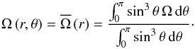 (1)Then, we
introduce the macroscopic velocity field, which is split into four components,
(1)Then, we
introduce the macroscopic velocity field, which is split into four components,
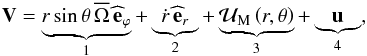 (2)with
 , where
k = {r,θ,ϕ} are the unit vectors in the radial,
latitudinal, and azimuthal directions. Term 1 represents the azimuthal velocity field
associated with shellular differential rotation. Term 2 corresponds to the Lagrangian
velocity due to the structural readjustments of the star during its evolution. Term 3 is
the meridional circulation velocity field that expands only on the ℓ = 2
spherical function for a shellular rotation
, where
k = {r,θ,ϕ} are the unit vectors in the radial,
latitudinal, and azimuthal directions. Term 1 represents the azimuthal velocity field
associated with shellular differential rotation. Term 2 corresponds to the Lagrangian
velocity due to the structural readjustments of the star during its evolution. Term 3 is
the meridional circulation velocity field that expands only on the ℓ = 2
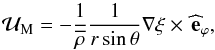
spherical function for a shellular rotation ![\begin{equation} {\vec {\mathcal U}}_{\rm M}=U_2\left(r\right)P_2\left(\cos\theta\right){\widehat {\vec e}}_r+\frac{1}{6{\overline\rho}r}\frac{{\rm d}}{{\rm d}r}\left[{\overline\rho} r^2 U_2\right]\frac{{\rm d}P_2\left(\cos\theta\right)}{{\rm d}\theta}\,{\widehat {\vec e}}_{\theta}. \label{MCexp} \end{equation}](/articles/aa/full_html/2013/10/aa21934-13/aa21934-13-eq11.png) (3)The latitudinal
component is obtained using the anelastic approximation, i.e.
(3)The latitudinal
component is obtained using the anelastic approximation, i.e.
 (
( is the mean
density on an isobar, cf. Eq. (7)), where
acoustic waves have been filtered out. Moreover, this approximation also allows
is the mean
density on an isobar, cf. Eq. (7)), where
acoustic waves have been filtered out. Moreover, this approximation also allows
 to be expressed as a function of a stream function
(ξM(r,θ))
as in Paper I,
to be expressed as a function of a stream function
(ξM(r,θ))
as in Paper I,
 (4)with
 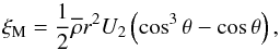 (5)where
is tangent to the iso-ξ line since
(5)where
is tangent to the iso-ξ line since
 .
This large-scale meridional circulation is driven by external torques such as those
associated to stellar winds or tides if there is a companion close to the considered star,
and by internal stresses (Zahn 1992; Maeder & Meynet 2000; Rieutord 2006; Decressin et al.
2009b).
.
This large-scale meridional circulation is driven by external torques such as those
associated to stellar winds or tides if there is a companion close to the considered star,
and by internal stresses (Zahn 1992; Maeder & Meynet 2000; Rieutord 2006; Decressin et al.
2009b).
We introduce through Term 4 the IGWs velocity field (Zahn et al. 1997) ![\begin{eqnarray} {\vec u}\left(r,\theta,\varphi,t\right)&=&\sum_{\sigma,\ell,m}\Big\{\left[u_{r;\ell}\left(r\right)Y_{\ell}^{m}\left(\theta,\varphi\right)+u_{H;\ell}\left(r\right){\vec\nabla}_{H}Y_{\ell}^{m}\left(\theta,\varphi\right)\right] \nonumber\\ &&\times \exp[-{\rm i}\sigma\,t]\Big\} \end{eqnarray}](/articles/aa/full_html/2013/10/aa21934-13/aa21934-13-eq20.png) (6)that
is expanded in spherical harmonics where ℓ and m are,
respectively, the classical orbital and azimuthal numbers. Here,
m > 0 and
m < 0 correspond to prograde and retrograde
IGWs, respectively and σ is the wave frequency. Finally, we introduce the
horizontal gradient
(6)that
is expanded in spherical harmonics where ℓ and m are,
respectively, the classical orbital and azimuthal numbers. Here,
m > 0 and
m < 0 correspond to prograde and retrograde
IGWs, respectively and σ is the wave frequency. Finally, we introduce the
horizontal gradient  .
.
Moreover, each scalar field (X) is written as  (7)with
its horizontal average on an isobar (
(7)with
its horizontal average on an isobar ( ) and its
associated fluctuation δX that is expanded in the ℓ = 2
spherical function because of the choice of a shellular rotation. In particular, we expand
the temperature
) and its
associated fluctuation δX that is expanded in the ℓ = 2
spherical function because of the choice of a shellular rotation. In particular, we expand
the temperature ![\begin{equation} T\left(r,\theta\right)={\overline T}\left(r\right)+\delta T\left(r,\theta\right)\,\,\,\hbox{with}\,\,\, \delta T=\left[\Psi_{2}\left(r\right){\overline T}\right]P_{2}\left(\cos\theta\right) \end{equation}](/articles/aa/full_html/2013/10/aa21934-13/aa21934-13-eq31.png) (8)and
the mean molecular weight
(8)and
the mean molecular weight ![\begin{equation} \mu\left(r,\theta\right)={\overline \mu}\left(r\right)+\delta \mu\left(r,\theta\right)\quad\hbox{with}\quad \delta \mu=\left[\Lambda_{2}\left(r\right){\overline \mu}\right]P_{2}\left(\cos\theta\right) \end{equation}](/articles/aa/full_html/2013/10/aa21934-13/aa21934-13-eq32.png) (9)with
Ψ2 and Λ2 their relative fluctuations on the isobar.
(9)with
Ψ2 and Λ2 their relative fluctuations on the isobar.
Finally, the unresolved scales that mostly correspond to the turbulent transport, are described by prescriptions coming from laboratory experiments or numerical simulations and if not from phenomenological considerations (see Sect. 2.6).
2.2. Internal gravity waves
2.2.1. Transport of angular momentum by internal gravity waves
Internal gravity waves are excited both by convective penetration in stable regions (Garcia Lopez & Spruit 1991; Kiraga et al. 2003, 2005; Browning et al. 2004; Dintrans et al. 2005; Rogers & Glatzmaier 2005, 2006; Brun et al. 2011) and in the bulk of convective regions by Reynolds stresses and buoyancy (Goldreich & Kumar 1990; Kumar & Quataert 1997; Belkacem et al. 2009; Samadi et al. 2010,see Sect. 2.2.2). They transport angular momentum and deposit it in the radiative layers at the depth where they are damped in a corotation resonance (Goldreich & Nicholson 1989; Zahn et al. 1997). This modifies the angular velocity of the stars, their internal differential rotation, and their evolution because of the induced modification of internal mixing (Talon et al. 2002; Talon & Charbonnel 2003, 2004, 2005).
Here, we summarize the formalism based on Zahn et al.
(1997) that was initially implemented in the stellar evolution code STAREVOL by
Talon & Charbonnel (2005). First, we
recall that the local momentum luminosity is related to the flux of angular momentum
transported by Reynolds stresses caused by IGWs (FJ)
 (10)with
 .
Assuming both the Jeffreys-Wentzel-Kramers-Brillouin and the quasi-linear assumptions
for IGWs (see the detailed discussion in Rogers et al.
2008; Mathis 2009), we write
.
Assuming both the Jeffreys-Wentzel-Kramers-Brillouin and the quasi-linear assumptions
for IGWs (see the detailed discussion in Rogers et al.
2008; Mathis 2009), we write
![\begin{equation} {\mathcal L}_{\rm J}\left(r\right)=\sum_{\sigma,\ell,m}{\mathcal L}_{{\rm J};\ell,m}\left(r_{\rm c},\sigma\right)\exp\left[-\tau_{l}\left(r,{\widehat\sigma}\right)\right], \label{LJ} \end{equation}](/articles/aa/full_html/2013/10/aa21934-13/aa21934-13-eq38.png) (11)where
rc is the radial position of the border of the convective
zone that excites IGWs and τℓ is the local
damping rate that takes into account the mean molecular weight stratification
(11)where
rc is the radial position of the border of the convective
zone that excites IGWs and τℓ is the local
damping rate that takes into account the mean molecular weight stratification
![\begin{equation} \tau_{\ell}=\left[\ell\left(\ell+1\right)\right]^{\frac{3}{2}}\int_{r}^{r_{\rm c}}K\frac{N\,N_{T}^{2}}{{\widehat\sigma}^4}\left(\frac{N^2}{N^2-{\widehat\sigma}^2}\right)^{\frac{1}{2}}\frac{{\rm d}r'}{r'^3}\,;\label{tau} \end{equation}](/articles/aa/full_html/2013/10/aa21934-13/aa21934-13-eq41.png) (12)K is
the thermal diffusivity, while
(12)K is
the thermal diffusivity, while  is the
total Brunt-Väisälä frequency; NT is the
buoyancy frequency linked to the entropy stratification given by
is the
total Brunt-Väisälä frequency; NT is the
buoyancy frequency linked to the entropy stratification given by
 with the usual notations for the temperature gradient
 and
pressure height scale
and
pressure height scale  ;
;
 is the
horizontal average of the effective gravity
is the
horizontal average of the effective gravity 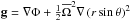 (Φ is the
gravitational potential); and
(Φ is the
gravitational potential); and 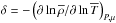 is
introduced by the used generalised equation of state (see Kippenhahn & Weigert 1990, for more details). Similarly,
Nμ is the buoyancy frequency related to
the chemical stratification given by
is
introduced by the used generalised equation of state (see Kippenhahn & Weigert 1990, for more details). Similarly,
Nμ is the buoyancy frequency related to
the chemical stratification given by  , where
 and
and
 . Finally,
 is the local Doppler-shifted frequency
 (13)where
σ is the excitation frequency in the reference frame of the
convection zone generating IGWs and ΩCZ corresponds to uniform rotation in
the convection zone.
(13)where
σ is the excitation frequency in the reference frame of the
convection zone generating IGWs and ΩCZ corresponds to uniform rotation in
the convection zone.
2.2.2. Volumetric generation of internal gravity waves by convective Reynolds stresses and buoyancy
In the present work, we follow Talon &
Charbonnel (2005) for the prescription for IGW excitation and adopt the
formalism of Goldreich et al. (1994) for acoustic
waves adapted by Kumar & Quataert (1997)
to describe volumetric stochastic excitation by turbulent convection (we do not consider
the possible effects of penetration by plumes, see Sect. 3.3). The momentum luminosity at the convective border is
 (14)where
FE;ℓ is the energy flux per unity
frequency
(14)where
FE;ℓ is the energy flux per unity
frequency ![\begin{eqnarray} {F}_{{\rm E};\ell}\left({r}_{\rm c},\sigma\right)&=&\frac{1}{4\pi}\int_{r_{\rm c}}^{R}\left\{\frac{\overline\rho^2}{r^2}\left[\left(\frac{{\rm d}\,u_{r;\ell}}{{\rm d}r}\right)^2+\ell\left(\ell+1\right)\left(\frac{{\rm d}\,u_{H;\ell}}{{\rm d}r}\right)^2\right]\right.\nonumber\\ &&{\left.\times\frac{V^3 L^4}{1+\left({\omega {\tau}_{L}}\right)^{15/2}}\exp\left[-\ell\left(\ell+1\right)\frac{h_{\sigma^2}}{2 r^2}\right]{\rm d}r\right\}}\, \label{RSE} \end{eqnarray}](/articles/aa/full_html/2013/10/aa21934-13/aa21934-13-eq61.png) (15)and
V is the convective velocity, L the radial size of
an energy bearing turbulent eddy,
τL ≈ L/V
the characteristic convective time, and
hσ = L min[1,(2 σ τL)−3/2]
the radial size of the largest eddy at depth r with characteristic
frequency σ or greater deduced from the mixing-length theory. The
excitation is computed at each evolution time-step and is therefore always fully
consistent with the stellar structure.
(15)and
V is the convective velocity, L the radial size of
an energy bearing turbulent eddy,
τL ≈ L/V
the characteristic convective time, and
hσ = L min[1,(2 σ τL)−3/2]
the radial size of the largest eddy at depth r with characteristic
frequency σ or greater deduced from the mixing-length theory. The
excitation is computed at each evolution time-step and is therefore always fully
consistent with the stellar structure.
The damping of each wave in the radiative zone is computed and then summed-up to obtain the total local momentum luminosity as in Eq. (11).
2.3. Transport of angular momentum and meridional circulation
We recall the equation for the evolution of the mean angular momentum when averaging the
azimuthal projection of the momentum equation over an isobar and including IGWs (see e.g.
Talon & Charbonnel 2005), 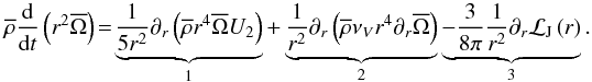 (16)\pagebreak
Term 1 represents the transport of angular momentum by meridional circulation, which
advective character is conserved. Term 2 is associated with the action of shear-induced
turbulence that is modelled as a diffusive process (see Sect. 2.6), where νV is the corresponding
turbulent viscosity in the vertical direction given in Eq. (37). Term 3 corresponds to the deposit/extraction of angular momentum
by IGWs described by Eq. (11). Finally,
the Lagrangian operator
d/dt = ∂t + ṙ∂r
accounts for contraction and dilatation of the star during its evolution (with the radial
velocity  ).
).
Equation (16) relates meridional circulation to the overall transport of angular momentum. In the asymptotic regime, the left-hand side term is zero and the transport of angular momentum by meridional circulation is exactly balanced by that through shear turbulence and IGWs. In the limit of vanishing turbulent viscosity and transport by IGWs, the rotation profile would adjust so that no meridional currents appear (Busse 1982). In reality, because of the extraction of angular momentum by magnetised wind (see below), and/or its redistribution by structural changes, the left-hand side term is non zero.
Then, following the method given in Paper I, and
integrating Eq. (16) over an isobar, we
get an equation for the fluxes of angular momentum as carried by the various involved
processes,  (17)where
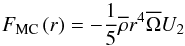 (18)is
the flux advected by the meridional circulation,
(18)is
the flux advected by the meridional circulation,
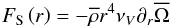 (19)is
that associated to the shear-induced turbulence, and
(19)is
that associated to the shear-induced turbulence, and
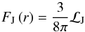 (20)is the
one deposited/extracted by IGWs. The term
(20)is the
one deposited/extracted by IGWs. The term  represents the loss or gain of angular momentum inside the isobar enclosing the mass
 (see Appendix A)
 ![\begin{equation} \Gamma \left(m\right) =\frac{1}{4\pi}\frac{\rm d}{{\rm d}t}\left[\int_{0}^{M\left(r\right)}{r'}^2{\overline\Omega}\,{\rm d}m'\right]. \end{equation}](/articles/aa/full_html/2013/10/aa21934-13/aa21934-13-eq77.png) (21)Then, using Eq.
(17), we can extract the radial function
of the vertical component of the meridional circulation velocity
(21)Then, using Eq.
(17), we can extract the radial function
of the vertical component of the meridional circulation velocity ![\begin{eqnarray} U_2&=&\frac{5}{{\overline\rho}r^4{\overline\Omega}}\left[\Gamma_M\left(r\right)-{\overline\rho}\nu_{\rm V} r^4 \partial_{r}\overline\Omega+\frac{3}{8\pi}{\mathcal L}_{\rm J}\right] \nonumber\\ &=&U_{\Gamma}+U_{V}+U_{{\mathcal L}_{\rm J}}. \label{U2} \end{eqnarray}](/articles/aa/full_html/2013/10/aa21934-13/aa21934-13-eq78.png) (22)Finally,
we note that we have the following boundary conditions at the top of radiative cores (RC)
of low-mass stars (
(22)Finally,
we note that we have the following boundary conditions at the top of radiative cores (RC)
of low-mass stars ( ),
),
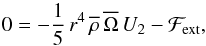
![\begin{equation} {{\rm d} \over {\rm d}t} \left[\int_{\,r_{t}^{\rm RC}}^{\,R}r'^{4}\,\overline\rho\,\overline\Omega\,{\rm d}r'\right]=-{1 \over 5}\,r^{4}\,{\overline\rho}\,\overline{\Omega}\,U_{2}-{\mathcal F}_{\rm ext}+\frac{3}{8\pi}{\mathcal L}_{\rm J}\left(r_{t}^{\rm RC}\right), \end{equation}](/articles/aa/full_html/2013/10/aa21934-13/aa21934-13-eq80.png) (23)where
ℱext is the flux of angular momentum carried by magnetic pressure-driven
stellar winds (Kawaler 1988; Pinto et al. 2011; Matt et al.
2012) and by tides if there is a close companion (Zahn 1977; Ogilvie & Lin
2007; Remus et al. 2012; Lai 2012) 1.
(23)where
ℱext is the flux of angular momentum carried by magnetic pressure-driven
stellar winds (Kawaler 1988; Pinto et al. 2011; Matt et al.
2012) and by tides if there is a close companion (Zahn 1977; Ogilvie & Lin
2007; Remus et al. 2012; Lai 2012) 1.
2.4. Thermal relaxation
Meridional circulation advects the mean entropy ( ) and the
temperature field relaxes on the new thermal state. The induced temperature fluctuation
) and the
temperature field relaxes on the new thermal state. The induced temperature fluctuation
 evolution
is ruled by the relaxation equation (Mathis & Zahn
2004)
evolution
is ruled by the relaxation equation (Mathis & Zahn
2004) ![\begin{eqnarray} \lefteqn{\underbrace{{\overline \rho}C_{p}\frac{\rm d}{{\rm d}t}{\widehat T}_2}_{{\overline\rho}{\overline T}\partial_{t}{\widetilde S}}-\left[\underbrace{{\overline \rho}\frac{L}{M}\left({\mathcal T}_{2,{\rm Th}}+{\mathcal T}_{2,{\mathcal B}}\right)}_{\vec\nabla\cdot\left(\chi\vec\nabla T\right)-\vec\nabla\cdot\vec F_{H}}\right]=}\nonumber\\ & &\underbrace{-{\overline \rho}{\overline T}C_{p}\frac{N_{T}^{2}}{{\overline g}}U_{2}}_{{\overline\rho}{\overline T}U_{r}\partial_{r}{\overline S}}+\underbrace{{\overline \rho}\frac{L}{M}{\mathcal T}_{2,{\rm N-G}}}_{\rho\varepsilon}. \label{eqMer} \end{eqnarray}](/articles/aa/full_html/2013/10/aa21934-13/aa21934-13-eq86.png) (26)This
is an advection/diffusion equation, where the advective term associated with meridional
circulation caused by the transport of angular momentum plays the role of a source or sink
of heat. The terms
(26)This
is an advection/diffusion equation, where the advective term associated with meridional
circulation caused by the transport of angular momentum plays the role of a source or sink
of heat. The terms  and
and  describe the usual spherical diffusion of heat and the component of the divergence of the
radiative flux due to the flattening of the isobar by the centrifugal acceleration;
∇·FH is the entropy flux carried by the
horizontal turbulence. Finally,
describe the usual spherical diffusion of heat and the component of the divergence of the
radiative flux due to the flattening of the isobar by the centrifugal acceleration;
∇·FH is the entropy flux carried by the
horizontal turbulence. Finally,  corresponds to the coupling with the nuclear energy generation. Their derivation may be
found in Paper I and are recalled in Appendix A.
corresponds to the coupling with the nuclear energy generation. Their derivation may be
found in Paper I and are recalled in Appendix A.
Equation (26) is finally written in the
following form, which will be used in Sect. 3.5.  (27)where
 (28)
(28) (29)
(29) (30)
(30) (31)
(31) (32)
(32)
2.4.1. The thermal wind equation
Next, once the temperature has relaxed, the new differential rotation profile is
obtained through the thermal wind equation 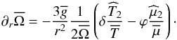 (33)A new eddy-viscosity
(νV) is thus obtained because of the modification of the
vertical gradient of angular velocity. To close the loop, the meridional circulation is
substained if there are some external torques, structural adjustments, and internal
stresses. If this is not the case, the circulation vanishes after an Eddington-Sweet
time
(33)A new eddy-viscosity
(νV) is thus obtained because of the modification of the
vertical gradient of angular velocity. To close the loop, the meridional circulation is
substained if there are some external torques, structural adjustments, and internal
stresses. If this is not the case, the circulation vanishes after an Eddington-Sweet
time ![\hbox{$t_{\rm ES}=\left[\frac{L R}{G M^2}\left(\frac{\Omega_{s}^{2}R^3}{GM}\right)\right]^{-1}$}](/articles/aa/full_html/2013/10/aa21934-13/aa21934-13-eq98.png) (Busse 1982; Rieutord 2006; Decressin et al. 2009b).
(Busse 1982; Rieutord 2006; Decressin et al. 2009b).
2.5. Transport of nuclides
We recall that the expansion of the transport equation for the nuclides on an isobar
leads to an equation for the evolution of the mass fraction of each considered chemical
(see also e.g. Meynet & Maeder 2000)
![\begin{eqnarray} \left(\frac{{\rm d} X_i}{{\rm d}t}\right)_{M_r}= \frac{\partial}{\partial M_r}\left[(4\pi r^2\rho)^2\left(D_{\rm V}+D_{\rm eff}\right) \frac{\partial X_i}{\partial M_r}\right] + \left(\frac{{\rm d}X_i}{{\rm d}t}\right)_{\rm nucl}, \label{Cmoy} \end{eqnarray}](/articles/aa/full_html/2013/10/aa21934-13/aa21934-13-eq99.png) (34)where
d
(34)where
d and
DV is the vertical component of the turbulent diffusivity
(see Eq. (37) below). The strong
horizontal turbulence leads to the erosion of the advective transport that can then be
described as a diffusive process (Chaboyer & Zahn
1992) with the effective diffusion coefficient
and
DV is the vertical component of the turbulent diffusivity
(see Eq. (37) below). The strong
horizontal turbulence leads to the erosion of the advective transport that can then be
described as a diffusive process (Chaboyer & Zahn
1992) with the effective diffusion coefficient 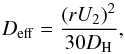 (35)where
DH is the horizontal component of the turbulent diffusivity
(see Eq. (38)). The second term on the
right-hand side of Eq. (34) corresponds to
the temporal mass fraction evolution of the ith nuclide due to nuclear
burning. In the present study we do not account for atomic diffusion.
(35)where
DH is the horizontal component of the turbulent diffusivity
(see Eq. (38)). The second term on the
right-hand side of Eq. (34) corresponds to
the temporal mass fraction evolution of the ith nuclide due to nuclear
burning. In the present study we do not account for atomic diffusion.
Equation (34) is complemented by an
equation for the time evolution of the relative fluctuation of the mean molecular weight,
expressed here in terms of Λ2: 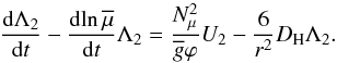 (36)We stress that
the advective character of the transport of angular momentum by the meridional circulation
and its deposit/extraction by IGWs makes the interpretation of the whole hydrodynamics
more complex than when the diffusive approximation is used (e.g. Pinsonneault et al. 1989; Heger et al.
2000). This is one of the reasons that pushed us to develop the tools that we
describe in Paper I and that we generalise in Sect.
3 to depict the action of IGWs.
(36)We stress that
the advective character of the transport of angular momentum by the meridional circulation
and its deposit/extraction by IGWs makes the interpretation of the whole hydrodynamics
more complex than when the diffusive approximation is used (e.g. Pinsonneault et al. 1989; Heger et al.
2000). This is one of the reasons that pushed us to develop the tools that we
describe in Paper I and that we generalise in Sect.
3 to depict the action of IGWs.
2.6. Turbulence and diffusion
The details of turbulence modelling have already been extensively discussed in previous papers, and we recall here the expressions we have chosen following again Talon & Charbonnel (2005).
First, for the vertical turbulent diffusion coefficients
(DV ≃ νV) we use the expression
by Talon & Zahn (1997), 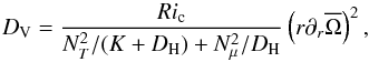 (37)where
Ric = 1/6 is the adopted
value for the critical Richardson number. This prescription is now supported by direct
numerical simulations of shear-induced turbulence (Prat
& Lignières 2013).
(37)where
Ric = 1/6 is the adopted
value for the critical Richardson number. This prescription is now supported by direct
numerical simulations of shear-induced turbulence (Prat
& Lignières 2013).
Next, for the horizontal turbulent viscosity we use the prescription derived by Zahn (1992),  (38)where
CH is a parameter of order unity, and
V2 is given by Eq. (3). For the vertical turbulent diffusion coefficient, we assume that
DH ≃ νH.
(38)where
CH is a parameter of order unity, and
V2 is given by Eq. (3). For the vertical turbulent diffusion coefficient, we assume that
DH ≃ νH.
3. Prescriptions for the 1.1 M⊙ Z⊙ stellar model computations
3.1. Basic input physics
In the following, we apply the formalism described in Sect. 2 to the main-sequence evolution of a rotating star with an initial mass of 1.1 M⊙ at solar metallicity. The model was computed with the implicit Lagrangian stellar evolution code STAREVOL V3.10, with the same basic input physics as Paper I and Lagarde et al. (2012,see these papers for details).
3.2. Rotation
We follow the evolution of the internal rotation profile from the zero age main sequence on, assuming initial solid body rotation, and an initial surface velocity of 75 km s-1 corresponding to 36% of the critical velocity (similar to Lagarde et al. 2012). We account for surface spin-down due to magnetic braking following the Kawaler (1988) formalism as described in Palacios et al. (2003) with a constant K = 2 × 1030.
Mass loss is included from the zero age main sequence following Reimers (1975) prescription with a parameter ηR = 0.5 (see also Palacios et al. 2006). Rotation effects on mass loss are accounted for following Maeder & Meynet (2001). Angular momentum losses associated with mass loss are also accounted for, but anisotropy effects (see Maeder 2002) are neglected. However, because of the low-mass loss rate during the main sequence, these effects are negligible.
3.3. Wave excitation and spectrum along the main sequence evolution
As the only convective zone in the 1.1 M⊙ main-sequence model is the envelope, we consider only waves generated by Reynolds stresses in this convective envelope. In the computations, we choose to multiply the kinetic energy flux obtained from the volumetric convective excitation by a factor of 5 in agreement with the results of Lecoanet & Quataert (2013) who show that the excitation by turbulent convection with a smooth transition at the radiative-convective transition leads to a flux about a factor of 5 higher than the one obtained by Eq. (15).
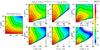 |
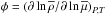
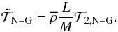
Fig. 1 Left: spectrum of the IGW luminosity generated by the convective Reynolds stresses of the envelope for various frequencies σ and degrees ℓ. Middle: spectrum of the IGW luminosity at 0.05 R⊙ below the convective envelope for retrograde (left) and prograde (right) waves with various frequencies and degrees ℓ. Only the cases with m = ℓ (top) and m = 1 (bottom) are shown. Right: spectrum of the net luminosity at 0.05 R⊙ below the convective envelope for various frequencies and degrees ℓ (and m). |
Figure 1 shows the luminosity spectrum of the IGWs generated by the convective envelope for the model at the age of 180 millions years. As already emphasized by Talon & Charbonnel (2005), the structure of the spectrum shows almost no variation along the main sequence. The left panel of Fig. 1 shows the spectrum of luminosity generated at the edge of the convective envelope. As already found by Talon & Charbonnel (2005), the waves which have the highest luminosity are those with small local frequency.
Moreover, as already pointed out by Talon & Charbonnel (2005) (see also Zahn et al. 1997), most of the waves are efficiently damped in the radiative region very close to the convective border. The central panels of Fig. 1 illustrate this point by showing the spectrum of wave luminosity at 0.05 R⊙ below the convective border. At that depth, retrograde and prograde waves with high degree ℓ and small frequency are already damped, and this effect is more pronounced for the prograde waves with azimuthal degree m = ℓ. For each frequency, and given degrees ℓ and m, the net luminosity is dominated by the retrograde waves where their maximum luminosity is limited to the area with small frequency and degree ℓ (see right panel of Fig. 1 and Eq. (12)).
4. Dynamical evolution of a 1.1 M⊙ Z⊙ star
In the following sections, we generalise the tools developed in Paper I to improve our understanding of the quantitative IGW effects on the transport of angular momentum and chemicals during the evolution of the 1.1 M⊙ model along the main sequence.
4.1. Rotation
4.1.1. Internal rotation profiles
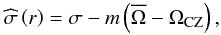
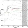 |
Fig. 2 Profiles of angular velocity in a 1.1 M⊙ star (Z = Z⊙) at different ages between 130 and 382 million years. The black, red, and green profiles at 180, 197, and 213 million years, respectively, indicate the time where we perform our analysis. Hatched area indicates the convective envelope. |
Figure 2 shows the evolution of the angular velocity profile between the zero age main sequence up to 382 million years where six extraction fronts have propagated to the surface. Talon & Charbonnel (2005) and Charbonnel & Talon (2005) explain that IGWs extract angular momentum at the depth they are damped. This depth moves toward the surface with time and then IGWs penetrate deeply into the star and a new extraction front starts. In our 1.1 M⊙, we obtain a similar behaviour. In the following we will concentrate our analysis on the third extraction front to study the changes in rotation and chemical transport as it propagates toward the surface. The three curves in black, red, and green, correspond to the rotation profile at the three times located in Fig. 3 where the extraction front moves outward at r = 0.15, 0.3 and 0.5 R⊙, respectively. Contrary to the general result obtained in the absence of IGWs (where only rotation, meridional circulation, and shear turbulence are taken into account) for a 1.1 M⊙ star (Z = Z⊙) and other solar-type star models, where we had a core spinning faster than the envelope (see e.g. Paper I), we obtain here a weak differential rotation because of its damping by IGWs and the related angular momentum extraction fronts (as in Talon & Charbonnel 2005).
4.1.2. Surface velocity
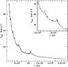 |
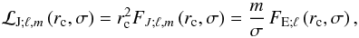
Fig. 3 Surface velocity of a 1.1 M⊙ star (Z = Z⊙), with an initial velocity of 75 km s-1 at the ZAMS. The bue squares at 180, 197, and 213 million years indicate the time at which the structures are detailed. |
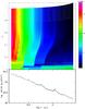 |
Fig. 4 Top: variation of the angular velocity
( |

Figure 3 shows the evolution of the surface velocity for the first 2.5 Gyr on the main sequence (the central hydrogen abundance decreases from 0.71 to 0.44). The surface velocity starts on the Zero-Age-Main-Sequence at 75 km s-1 and then it decreases because of magnetic braking to about 12−15 km s-1 at the Hyades ages, which is close to the velocity obtained by Gaige (1993) for star with a Teff around 5980 K: VHyades = 8 ± 10 km s-1. Thus the surface velocity reaches 5 km s-1 after 2.5 Gyr of evolution when most of the magnetic braking has occurred.
Along with this general decreasing trend, the surface velocity also shows a series of
small peaks, which are due to the arrival at the surface of extraction fronts induced by
the transport of angular momentum by IGWs (see Talon
& Charbonnel 2005). In Fig. 4, we
show the evolution of the rotation profile during the whole computed evolution, i.e.
 , along
with the loss of angular momentum due to magnetic braking. Then, we can clearly identify
the propagation of the different fronts of angular momentum extraction and their speed
of propagation which becomes slower and slower as the star evolves. This is due to the
strength of the magnetic wind and braking, which decreases with time. Therefore, less
differential rotation between the convective envelope and the internal core is
sustained. Then, the net bias between retrograde and prograde waves, which is fed by the
differential rotation reservoir, becomes less and less pronounced and the efficiency of
the extraction becomes less and less efficient and operates on longer time-scales.
, along
with the loss of angular momentum due to magnetic braking. Then, we can clearly identify
the propagation of the different fronts of angular momentum extraction and their speed
of propagation which becomes slower and slower as the star evolves. This is due to the
strength of the magnetic wind and braking, which decreases with time. Therefore, less
differential rotation between the convective envelope and the internal core is
sustained. Then, the net bias between retrograde and prograde waves, which is fed by the
differential rotation reservoir, becomes less and less pronounced and the efficiency of
the extraction becomes less and less efficient and operates on longer time-scales.
In the following, we follow in detail the propagation of the third extraction front at three different times (180, 197, and 213 million years) indicated by the blue squares in Fig. 3.
4.2. Sustaining the meridional circulation
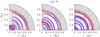 |
Fig. 5 Meridional circulation currents in a 1.1 M⊙ star (Z = Z⊙) model at 180 (left), 197 (middle), and 213 million years (right). Red and blue lines indicate counterclockwise and clockwise circulation, respectively. Hatched areas indicate the convective envelope. |
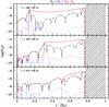 |
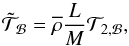
Fig. 6 Decomposition of the vertical component of the meridional circulation radial function U2 for a 1.1 M⊙ star (Z = Z⊙) at three different epochs indicated in each panel. Black long dashed lines show the value of U2, while red dashed-dotted, blue dotted, and magenta dashed lines indicate its different components ULJ, UV and UΓ, respectively (see Eq. (22)). Hatched areas indicate the convective envelope. |
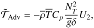
Figure 5 shows the two-dimensional reconstruction of the meridional circulation flows in the radiative interior. As in Paper I, they are represented in terms of the stream function ξ defined in Eq. (5). The striking difference with the models of 1.5 M⊙ presented in Paper I computed without IGWs is the presence of numerous small loops of meridional circulation instead of having only two loops with a large one connecting the surface to the deep interior. As shown by Talon & Charbonnel (2003), the efficiency of IGWs is ruled by the size of the convective envelope, which becomes negligible for stars above ~1.4 M⊙. For lower mass stars IGWs need to be taken into account. Models of a 1.1 M⊙ star without IGWs will show a similar pattern for the meridional circulation to the 1.5 M⊙ star shown in Paper I. In the 1.1 M⊙ star, where IGWs are taken into account, numerous loops of circulation are present with alternating clockwise and counterclockwise loops. As already noted by Talon & Charbonnel (2005), this meridional multi-loop pattern has a strong effect on the transport of angular momentum and chemicals that must be understood.
Figure 6 shows the reconstruction of the radial function of the vertical component of the meridional circulation (U2) based on Eq. (22) obtained from the conservation of angular momentum, where UΓ, UV, and the UℒJ represent the angular momentum extraction, the contribution of the shear, and of the one of Reynolds stresses caused by IGWs, respectively. We note that the contribution of IGWs is always positive (because of the net extraction of angular momentum) while the loops of meridional circulation have alternating positive and negative values. The propagation of the IGWs in the radiative interior and their damping create two main zones shown in Fig. 6. They are separated by the extraction front position at rextract = 0.12,0.3, and 0.5 R⊙ in the three panels. Above (between the convective envelope and the region where they are damped r ≥ rextract), the meridional circulation is sustained by the local variation of angular momentum given by UΓ and by the Reynolds stresses caused by IGWs given by UℒJ, i.e. U2 ≈ UΓ + UℒJ. Since UΓ is negative while UℒJ is positive with the same order of magnitude, we are thus able to understand the meridional circulation radial function (U2) amplitude, which can be alternatively positive and negative along the radius.
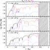 |
Fig. 7 Total flux of angular momentum (Ftot, black solid line) decomposed into the contributions due to the meridional circulation (FMC, red dashed line), the shear-induced turbulence (FS, blue dotted line), and the Reynolds stresses caused by IGWs (FJ, magenta dashed line) for a 1.1 M⊙ star (Z = Z⊙) at three different epochs indicated in each panel. Hatched areas indicate the convective envelope. |
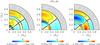 |
Fig. 8 Temperature fluctuation in the 1.1 M⊙ star (Z = Z⊙) model at 180 (left), 197 (middle) and 213 million years (right). Hatched areas indicate the convective envelope. |
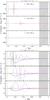 |
Fig. 9 Upper panels: heat transport for a 1.1
M⊙ star
(Z = Z⊙) at three different epochs
indicated in each panel with the terms non-stationary
( |

In the inner central part (r < rextract) where no IGWs are present because they have been damped near the extraction front, the meridional circulation is sustained mainly by the local variation of angular momentum given by UΓ as in Paper I, i.e. U2 ≈ UΓ.
The contribution of the shear (UV) is always negligible owing to the nearly-flat profile of rotation. The only place where the shear increases sharply is around the extraction front. However, as the other components of the meridional circulation are also highly excited in this place, the shear never becomes important although the rotation profile displays a stronger differential profile there. However, at the end of the main sequence evolution, once the wind becomes weak, the transport of angular momentum by IGWs is less efficient with extraction fronts of angular momentum that propagate more and more slowly (cf. Fig. 4). Then, once most of the angular momentum has been lost, a very weak meridional circulation is driven by the viscous stresses induced by the residual shear.
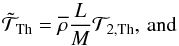
4.3. Flux of angular momentum
Here, we continue to examine the respective contribution of meridional circulation (FMC), shear (FS), and IGWs (FJ) to the total flux of angular momentum by looking at the fluxes carried by these three processes. Our analysis is presented in Fig. 7 for the three chosen structures of the propagation of the extraction front. We retrieve the similar pattern as in Fig. 6 where the radiative region can be decomposed into two regimes. In the inner one, below the extraction front (r < rextract), the transport of angular momentum is dominated by its advection by the meridional circulation, while above (r ≥ rextract), IGWs are the main conveyor. In the whole radiation zone, the diffusion of angular momentum by the shear-induced turbulence remains a secondary process.
Near the extraction front, the meridional circulation presents two important characteristics: a high value of its velocity and a double inversion peak (see Fig. 5) as a pattern with three fixed loops are present between 0.09–0.22, 0.18–0.42, and 0.5−0.68 R⊙ in the right, middle, and left panel, respectively. The two inner loops bring angular momentum from the outside to the extraction front while the outer one transports angular momentum outward. This typical pattern is responsible for the peak seen in the profile of angular momentum near the extraction front.
Moreover, as shown in Fig. 2, the profile of
 is frozen in
the region below the extraction front. This behaviour can be understood as follows. First,
the amplitude of the angular momentum flux stays almost constant where IGWs are the main
conveyor. Thus, angular momentum is efficiently extracted from the front to the convective
envelope and hence this process moves the front to higher radius. Second, in the inner
part, the total flux drops by several orders of magnitude compared to the region above and
the succession of clockwise and counterclockwise loops of meridional circulation halts the
transport of angular momentum. The net effect of these two mechanisms freezes the
evolution of angular momentum in the inner part compared to the time needed by the front
to move toward the surface.
is frozen in
the region below the extraction front. This behaviour can be understood as follows. First,
the amplitude of the angular momentum flux stays almost constant where IGWs are the main
conveyor. Thus, angular momentum is efficiently extracted from the front to the convective
envelope and hence this process moves the front to higher radius. Second, in the inner
part, the total flux drops by several orders of magnitude compared to the region above and
the succession of clockwise and counterclockwise loops of meridional circulation halts the
transport of angular momentum. The net effect of these two mechanisms freezes the
evolution of angular momentum in the inner part compared to the time needed by the front
to move toward the surface.
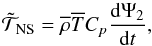
4.4. Entropy transport
Figure 8 displays the two-dimensional reconstruction
of the temperature perturbation (δT) in the meridional plane at different
ages along the evolution. Its behaviour is closely related to the gradients of angular
momentum; near the extraction front where steep gradients occur, δT
presents its maximum values. Furthermore, the value of the perturbations always remains
small as  is lower than
0.1%. This result validates our perturbation analysis.
is lower than
0.1%. This result validates our perturbation analysis.
Figure 9 (both panels) depicts how the thermal
relaxation in the heat transport equation is achieved. In Paper I, we showed that in the absence of IGWs the advection of entropy by the
meridional circulation ( ) is
compensated both by the thermal (
) is
compensated both by the thermal ( ) and
barotropic (
) and
barotropic ( ) components of
the radiative flux. The situation is quite different with the presence of IGWs because the
main peak of entropy advection by the meridional circulation (see Fig. 6) near the extraction front is solely balanced by the
thermal component. In the last panel of Fig. 9 (top),
the heat transport is weak and all the components have small values because the front we
are following arrives at the surface and a new one will be created. The bottom panel of
Fig. 9 shows the different components of the heat
transport equation with a zoom in the region outside the extraction front. There, the
advection of heat by the meridional circulation is still balanced by the thermal
component. However, the barotropic component induces some modulation. The nuclear and
gravitational energy generation term (
) components of
the radiative flux. The situation is quite different with the presence of IGWs because the
main peak of entropy advection by the meridional circulation (see Fig. 6) near the extraction front is solely balanced by the
thermal component. In the last panel of Fig. 9 (top),
the heat transport is weak and all the components have small values because the front we
are following arrives at the surface and a new one will be created. The bottom panel of
Fig. 9 shows the different components of the heat
transport equation with a zoom in the region outside the extraction front. There, the
advection of heat by the meridional circulation is still balanced by the thermal
component. However, the barotropic component induces some modulation. The nuclear and
gravitational energy generation term ( ) plays a
role only in the central region below 0.1−0.2 R⊙. Finally, the
non-stationary term (
) plays a
role only in the central region below 0.1−0.2 R⊙. Finally, the
non-stationary term ( ) is
negligible as it is mainly sensitive to the structural changes of the star, which remain
small during the main sequence.
) is
negligible as it is mainly sensitive to the structural changes of the star, which remain
small during the main sequence.
4.5. Effects on chemicals
4.5.1. Horizontal chemical unbalance
Figure 10 displays the two-dimensional reconstruction of horizontal fluctuations of mean molecular weight (μ). Nuclear burning increases the mean molecular weight in the centre and creates a negative vertical gradient. Then, the meridional circulation creates horizontal gradients when clockwise loops bring matter with low μ from the outside near the equatorial plane and push high μ matter along the pole from the centre to the outer regions. The reverse happens with counterclockwise loops. These μ perturbations tend to be erased by the horizontal turbulence.
Because of the numerous loops of meridional circulation we would expect the behaviour of the μ perturbations to be erratic. While Fig. 10 mainly confirms it, we can still identify some long-lived patterns. We see that the inner μ perturbations located at r = 0.10 R⊙ remain at the three times. This comes from the initial μ perturbations that are protected by clockwise loops that stay at this radius at all three times (see Fig. 5). Furthermore, as the horizontal diffusion is also weaker near the stellar centre (see Fig. 11), the initial μ perturbation is eroded on a longer timescale while the pattern above 0.10 R⊙ changed more rapidly.
4.5.2. Transport of chemicals
Figure 11 compares the diffusion coefficients of the various processes that act on the transport of chemicals. First, the horizontal turbulent transport is stronger than the vertical (i.e. DH ≫ DV) as expected from the shellular rotation hypothesis. Then, because of the very little vertical gradient of angular velocity, the vertical shear is weak except near the extraction front. The effective diffusion by meridional circulation and horizontal turbulence (Deff) follows the loops of the circulation. Therefore, the net effect is a strong reduction of the vertical mixing compared to the model presented in Paper I. Similar results have been obtained by Talon & Charbonnel (2005). These differences in the diffusion coefficient lead to a lower efficiency of the transport of light elements like Li near the convective envelope. As shown by Talon & Charbonnel (2003), gravity waves can inhibit the Li depletion on the cool side of the Li dip observed in open clusters (see e.g. Burkhart & Coupry 2000).
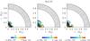 |
Fig. 10 Two-dimensional reconstruction of the μ fluctuations in the 1.1 M⊙ star (Z = Z⊙) model at 180 (left), 197 (middle), and 213 million years (right). Hatched areas indicate the convective envelope. |
5. Conclusions and perspectives
In this article, we generalised the work in Paper I aimed at unravelling secular transport and mixing processes in stellar radiation zones during the main sequence taking IGW actions into account. Using the STAREVOL code where the formalisms by Mathis & Zahn (2004) and Talon & Charbonnel (2005) are implemented, we simulated the evolution of a 1.1 M⊙, Z⊙ star focussing on the highly non-linear interaction between differential rotation, large-scale meridional circulation, shear-induced turbulence and IGWs. In our work, the non-diffusive character of angular momentum transport by the meridional circulation and IGWs is preserved. Then, using our generalised diagnoses, we identify that the meridional flows are driven by the external torque applied on the stellar surface by stellar winds and by IGWs and viscous stresses rather than by thermal imbalance (see also Busse 1982; Rieutord 2006) (stellar structure adjustments are also important, but not on the evolution phases we have studied in this work). This precise analysis now allows us to explain the highly multi-cellular meridional circulation already identified by Talon & Charbonnel (2005) and shows that the usual Eddington-Sweet vision of this flow must be abandoned. We note that this forcing of mean meridional and zonal flows by IGWs also occurs in the atmosphere of the Earth and the other planets (e.g. Holton 1982; Fritts & Alexander 2003). We then clarified the precise way IGWs act on the large-scale dynamics for angular momentum, heat, and chemical transports.
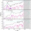 |
Fig. 11 Profiles of the thermal diffusivity (K; cyan dashed-dotted lines), and the diffusion coefficient associated with the meridional circulation (Deff; red dashed lines), and with the horizontal (DH; black long dashed lines) and vertical turbulence (DV; blue dotted lines) for a 1.1 M⊙ star (Z = Z⊙) at three different epochs indicated in each panel. The total diffusion coefficient used for the mixing of chemicals is indicated with magenta full lines. Hatched areas indicate the convective envelope. |
 |
Fig. 12 Secular hydrodynamics of stellar radiation zones taking into account IGWs actions (here, in the green box). The action of differential rotation through the Doppler shift is represented in blue. |
First, as in Talon & Charbonnel (2005), we unraveled the dynamics of angular momentum extraction fronts that propagate from the centre to the surface of the star. We note that the velocity of their propagation decreases along the evolution of the star during which surface braking by stellar winds becomes less efficient. Indeed, the corresponding applied torque sustains the differential rotation between the convective envelope of the star and its radiative core. This feeds the IGW action because of the different Doppler-shift of pro- and retrograde waves from which a net transport of angular momentum results. Then, once most of the differential rotation has been damped, a very weak meridional circulation is driven by the viscous stresses induced by the residual shear as described in Paper I. Next, heat and chemical transports are strongly affected by IGW action because of the related modification of the meridional circulation behaviour. Then, the meridional circulation advects entropy (and chemicals) and the star relaxes into a new thermal state. This in turn generates a new differential rotation profile because of the induced baroclinic torque (see Eq. (33)) and the related thermal wind (see Fig. 12).
The main improvments that should be added to this work in the near future mainly consist of improvments in the treatment of the excitation, propagation, and damping of IGWs.
First, for IGW amplitude, we here assume the prescription given by Kumar & Quataert (1997) for their volumetric stochastic excitation. However, progress has been achieved both analytically (Belkacem et al. 2009; Samadi et al. 2010) and using non-linear numerical simulations (Kiraga et al. 2005; Browning et al. 2004; Dintrans et al. 2005; Rogers & Glatzmaier 2005, 2006; Brun et al. 2011; Alvan et al. 2012) for the volumetric excitation and the surface excitation due to turbulent plumes. In the near future, it will thus be particularly important to extract usable prescriptions for excited IGW spectra from these works and to implement it in STAREVOL. Furthermore, as in the present implementation, it will be important to have appropriate prescriptions for each evolution phase where convective region properties evolve (see Talon & Charbonnel 2008; Charbonnel et al. 2013).
Next, we have ignored the action of the Coriolis acceleration and the Lorentz force (due to the dynamo field at the level of the excitation region at convection/radiation borders and/or to a fossil field in the bulk of stellar radiation zones) on IGWs. Both rotation and magnetic fields modify their propagation and damping, as well as the related transport of angular momentum and mixing, particularly for IGWs that are excited with frequencies close to the inertial frequency (2Ω) and to the Alfvén frequency (see Pantillon et al. 2007; Mathis et al. 2008a; Mathis 2009) for the action of the Coriolis acceleration and Mathis & de Brye (2011, 2012) for the combined action of rotation and magnetic fields); for example, equatorial trappings occur for these low-frequency IGWs. However, as has been demonstrated by Mathis & de Brye (2012), the net bias between pro- and retrograde waves that leads to the efficient extraction of angular momentum in solar-type stars by IGWs is conserved even when both the Coriolis acceleration and the Lorentz force are taken into account. It will be thus important to implement, step by step, their action on IGWs to get the complete interaction between IGWs and the large-scale dynamical processes in stellar radiation regions.
Finally, the torques applied at the surface of the star have an important impact on the internal transport processes. If the prescription by Kawaler (1988) is adopted here, it will be important to improve the prescriptions used for this torque, for example using the prescriptions obtained from three-dimensional simulations of stellar winds where the dependence of the wind on the rotation rate of the star is taken into account (Matt et al. 2012).
All of these theoretical improvments of our vision of the dynamical evolution of stars will benefit from constraints coming from seismology and surface abundance observations of the whole Hertzsprung-Russell diagram.
Appendix A: Meridional circulation and angular momentum transport
We consider Eq. (16) for the mean angular
momentum transport  (39)that
takes IGW action into account. We integrate it over a spherical shell
(39)that
takes IGW action into account. We integrate it over a spherical shell
 (40)where
r1 and r2 are, respectively, its
inner and outer radius. Introducing the elementary mass element
(40)where
r1 and r2 are, respectively, its
inner and outer radius. Introducing the elementary mass element
 , we obtain
![\begin{eqnarray} \lefteqn{\frac{1}{4\pi}\int_{m=m\left(r_1\right)}^{m=m\left(r_2\right)}\frac{\rm d}{{\rm d}t}\left({r'}^{2}\overline{\Omega}\right){\rm d}m=\frac{1}{5}\left[\left({\overline\rho} r^4 \overline{\Omega} U_{2}\right)_{r\,=\,r_2}-\left({\overline\rho} r^4 \overline{\Omega} U_{2}\right)_{r\,=\,r_1}\right]}\nonumber\\ &+&\left[\left({\overline\rho}\nu_{V}r^4\partial_{r}\overline{\Omega}\right)_{r\,=\,r_2}-\left({\overline\rho}\nu_{V}r^4\partial{r}\overline{\Omega}\right)_{r\,=\,r_1}\right]\nonumber\\ &-&\frac{3}{8\pi}\left[{\mathcal L}_{J}\left(r\,=\,r_2\right)-{\mathcal L}_{J}\left(r\,=\,r_1\right)\right]. \end{eqnarray}](/articles/aa/full_html/2013/10/aa21934-13/aa21934-13-eq165.png) (41)We
apply the following identity
(41)We
apply the following identity ![\begin{eqnarray*} \lefteqn{\frac{\rm d}{{\rm d}t}\left[\int_{m_1\left(t\right)}^{m_2\left(t\right)}f(m,t){\rm d}m\right]=\int_{m_1\left(t\right)}^{m_2\left(t\right)}\frac{\rm d}{{\rm d}t}\left[f(m,t)\right]{\rm d}m}\nonumber\\ &+&\left\{\frac{{\rm d}m_2\left(t\right)}{{\rm d}t} f\left(m_2,t\right)-\frac{{\rm d}m_1\left(t\right)}{{\rm d}t} f\left(m_1,t\right)\right\}.\nonumber\\ \end{eqnarray*}](/articles/aa/full_html/2013/10/aa21934-13/aa21934-13-eq166.png) In
our Lagrangian description, the mass is conserved, i.e.
In
our Lagrangian description, the mass is conserved, i.e.
 , so
, so ![\begin{eqnarray} \lefteqn{\frac{1}{4\pi}\frac{{\rm d}}{{\rm d}t}\left[\int_{m=m\left(r_1\right)}^{m=m\left(r_2\right)}r'^{2}\overline{\Omega}{\rm d}m\right]=\frac{1}{5}\left[\left({\overline\rho} r^4 \overline{\Omega} U_{2}\right)_{r\,=\,r_2}-\left({\overline\rho} r^4 \overline{\Omega} U_{2}\right)_{r\,=\,r_1}\right]}\nonumber\\ &+&\left[\left({\overline\rho}\nu_{V}r^4\partial_{r}\overline{\Omega}\right)_{r\,=\,r_2}-\left({\overline\rho}\nu_{V}r^4 \partial_{r}\overline{\Omega}\right)_{r\,=\,r_1}\right]\nonumber\\ &-&\frac{3}{8\pi}\left[{\mathcal L}_{J}\left(r\,=\,r_2\right)-{\mathcal L}_{J}\left(r\,=\,r_1\right)\right]. \label{Bilan} \end{eqnarray}](/articles/aa/full_html/2013/10/aa21934-13/aa21934-13-eq168.png) (42)Finally,
to obtain the value of the radial function of the vertical component of the meridional
circulation at ,
we set r1 = 0 and
r2 = r that leads to
(42)Finally,
to obtain the value of the radial function of the vertical component of the meridional
circulation at ,
we set r1 = 0 and
r2 = r that leads to
![\begin{equation} U_{2}=\frac{5}{{\overline\rho} r^4 \overline{\Omega}}\left[\Gamma\left(m\right)-{\overline\rho}\nu_{V}r^4\partial_{r}\overline{\Omega}+\frac{3}{8\pi}{\mathcal L}_{J}\left(r\right)\right], \end{equation}](/articles/aa/full_html/2013/10/aa21934-13/aa21934-13-eq171.png) (43)where
(43)where
![\begin{equation} \Gamma\left(m\right)=\frac{1}{4\pi}\frac{\rm d}{{\rm d}t}\left[\int_{0}^{m\left(r\right)}{r'}^2\overline{\Omega}{\rm d}m'\right]. \end{equation}](/articles/aa/full_html/2013/10/aa21934-13/aa21934-13-eq172.png) (44)
(44)
Appendix
B:
 components of the heat transport
equation
components of the heat transport
equation
This is an advection/diffusion equation, where the advective term associated with the
meridional circulation caused by the transport of angular momentum plays the role of a
source or sink of heat. The terms
and
describe the usual spherical diffusion of heat and the component of the divergence of the
radiative flux due to the flattening of the isobar by the centrifugal acceleration;
∇·FH is the entropy flux carried by the horizontal turbulence.
Finally,
corresponds to the coupling with the nuclear energy generation. Their derivation may be
found in Decressin et al. (2009) and we obtain the thermic term ![\begin{eqnarray} {\mathcal T}_{2,{\rm Th}}=\frac{\rho_{m}}{\overline{\rho}}\left[\frac{r}{3}\partial_{r}{\cal{A}}_{2}\left(r\right) -\frac{2 H_{T}}{3 r}\left(1 + \frac{D_{\rm H}}{K}\right)\frac{{\widehat T}_2}{\overline T}\right]\nonumber, \label{Tth} \end{eqnarray}](/articles/aa/full_html/2013/10/aa21934-13/aa21934-13-eq175.png) the
barotropic term
the
barotropic term ![\begin{eqnarray} \lefteqn{{\mathcal T}_{2,{\mathcal B}}=}\nonumber\\ &&\frac{2}{3}\left[1-\frac{\overline\Omega^2}{2\pi G\overline{\rho}}-\frac{2}{3}\frac{\rho_m}{\rho}\left(\phi\frac{{\widehat\mu}_2}{\overline\mu}-\delta\frac{{\widehat T}_2}{\overline T}\right)-\frac{\left(\overline{\epsilon}+\overline{\epsilon}_{\rm grav}\right)}{\epsilon_{m}}\right]\overline\Omega^{2}\partial_{r}\left(\frac{r^2}{\overline g}\right)\nonumber\\ &&-\frac{2}{3}\frac{\rho_m}{\overline\rho}\left(\phi\frac{{\widehat\mu}_2}{\overline\mu}-\delta\frac{{\widehat T}_2}{\overline T}\right)\nonumber, \label{TB} \end{eqnarray}](/articles/aa/full_html/2013/10/aa21934-13/aa21934-13-eq176.png) and
the term associated with local energy sources
and
the term associated with local energy sources ![\begin{eqnarray} {\mathcal T}_{2,{\rm N-G}}&=&\frac{\left(\overline{\epsilon}+\overline{\epsilon}_{\rm grav}\right)}{\epsilon_{m}}\left[{\cal{A}}_{2}\left(r\right)+\left(f_{\epsilon}\epsilon_{T} - f_{\epsilon}\delta + \delta\right)\frac{{\widehat T}_2}{\overline T}\right.\nonumber\\ &&{\left.+\left(f_{\epsilon}\epsilon_{\mu}+f_{\epsilon}\phi - \phi\right)\frac{{\widehat\mu}_2}{\overline\mu}\right]}\nonumber, \end{eqnarray}](/articles/aa/full_html/2013/10/aa21934-13/aa21934-13-eq177.png) where
where
 (45)and
L and M have their usual meanings. We have introduced
the temperature scale-height
(45)and
L and M have their usual meanings. We have introduced
the temperature scale-height  ,
the horizontal eddy-diffusivity DH and
,
the horizontal eddy-diffusivity DH and
 ,
with
,
with  and
and
 being the
mean nuclear and gravitational energy release rates, respectively;
being the
mean nuclear and gravitational energy release rates, respectively;
 and
and  are the logarithmic derivatives of
  and of the
radiative conductivity χ with respect to
and of the
radiative conductivity χ with respect to
 , and
, and
 and
and  are the derivatives of these same quantities with respect to
 ;
ϵm = L/M
and
;
ϵm = L/M
and  are the horizontal
average of the energy production rate and the mean density inside the considered isobar.
Finally, the signature of mixing induced by transport processes, i.e. the fluctuation of the
mean molecular weight
are the horizontal
average of the energy production rate and the mean density inside the considered isobar.
Finally, the signature of mixing induced by transport processes, i.e. the fluctuation of the
mean molecular weight 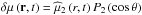 , has
been introduced.
, has
been introduced.
We also note that for massive stars, we will have at the top of radiative envelopes (RE)
( )
)
where ℱext is the flux of angular momentum carried by radiative
stellar winds (Ud-Doula et al. 2009; Meynet et al. 2011) and tides and at the top of a
convective core (CC) ( )
)
![\begin{equation} {{\rm d} \over {\rm d}t} \left[\int_{\,0}^{\,r_{\rm t}^{\rm CC}}r'^{4}\,\overline\rho\,\overline\Omega\,{\rm d}r'\right]=\frac{1}{5}\,r^{4}\,{\overline\rho}\,\overline{\Omega}\,U_{2}-\frac{3}{8\pi}\mathcal{L}_{\rm J}\left(r_{\rm t}^{\rm CC}\right). \end{equation}](/articles/aa/full_html/2013/10/aa21934-13/aa21934-13-eq83.png)
Acknowledgments
T.D. and C.C. acknowledge financial support from the Swiss National Science Foundation (FNS) and from ESF-Eurogenesis. This work was also supported by the French Programme National de Physique Stellaire (PNPS) of CNRS/INSU, by the CNES-SOHO/GOLF grant and asteroseismology support in CEA-Saclay, and by the TOUPIES project funded by the French National Agency for Research (ANR). S.M. is grateful to Geneva Observatory where part of this work has been realized.
References
- Aerts, C., Thoul, A., Daszyńska, J., et al. 2003, Science, 300, 1926 [NASA ADS] [CrossRef] [PubMed] [Google Scholar]
- Alvan, L., Brun, A. S., & Mathis, S. 2012, in SF2A-2012: Proceedings of the Annual meeting of the French Society of Astronomy and Astrophysics, eds. S. Boissier, P. de Laverny, N. Nardetto, et al., 289 [Google Scholar]
- Beck, P. G., Montalban, J., Kallinger, T., et al. 2012, Nature, 481, 55 [NASA ADS] [CrossRef] [Google Scholar]
- Belkacem, K., Samadi, R., Goupil, M. J., et al. 2009, A&A, 494, 191 [NASA ADS] [CrossRef] [EDP Sciences] [Google Scholar]
- Bouvier, J. 2008, A&A, 489, L53 [NASA ADS] [CrossRef] [EDP Sciences] [Google Scholar]
- Browning, M. K., Brun, A. S., & Toomre, J. 2004, ApJ, 601, 512 [NASA ADS] [CrossRef] [Google Scholar]
- Brun, A. S., Miesch, M. S., & Toomre, J. 2011, ApJ, 742, 79 [NASA ADS] [CrossRef] [Google Scholar]
- Burkhart, C., & Coupry, M. F. 2000, A&A, 354, 216 [NASA ADS] [Google Scholar]
- Busse, F. H. 1982, ApJ, 259, 759 [NASA ADS] [CrossRef] [Google Scholar]
- Ceillier, T., Eggenberger, P., García, R. A., & Mathis, S. 2012, Astron. Nachr., 333, 971 [NASA ADS] [CrossRef] [Google Scholar]
- Chaboyer, B., & Zahn, J.-P. 1992, A&A, 253, 173 [NASA ADS] [Google Scholar]
- Decressin, T., Baumgardt, H., Kroupa, P., Meynet, G., & Charbonnel, C. 2009a, in The ages of stars, ed. D. Soderblom, IAU Symp., 258 [Google Scholar]
- Charbonnel, C., & Talon, S. 2005, Science, 309, 2189 [NASA ADS] [CrossRef] [PubMed] [Google Scholar]
- Charbonnel, C., Decressin, T., Amard, L., Palacios, A., & Talon, S. 2013, A&A, 554, A40 [NASA ADS] [CrossRef] [EDP Sciences] [Google Scholar]
- Decressin, T., Mathis, S., Palacios, A., et al. 2009b, A&A, 495, 271 [NASA ADS] [CrossRef] [EDP Sciences] [Google Scholar]
- Deheuvels, S., García, R. A., Chaplin, W. J., et al. 2012, ApJ, 756, 19 [NASA ADS] [CrossRef] [Google Scholar]
- Dintrans, B., Brandenburg, A., Nordlund, Å., & Stein, R. F. 2005, A&A, 438, 365 [NASA ADS] [CrossRef] [EDP Sciences] [Google Scholar]
- Eff-Darwich, A., & Korzennik, S. G. 2012, Sol. Phys., 149 [Google Scholar]
- Eggenberger, P., Maeder, A., & Meynet, G. 2005, A&A, 440, L9 [NASA ADS] [CrossRef] [EDP Sciences] [Google Scholar]
- Eggenberger, P., Meynet, G., Maeder, A., et al. 2008, Ap&SS, 316, 43 [NASA ADS] [CrossRef] [Google Scholar]
- Eggenberger, P., Montalbán, J., & Miglio, A. 2012, A&A, 544, L4 [NASA ADS] [CrossRef] [EDP Sciences] [Google Scholar]
- Espinosa Lara, F., & Rieutord, M. 2007, A&A, 470, 1013 [NASA ADS] [CrossRef] [EDP Sciences] [Google Scholar]
- Fritts, D. C., & Alexander, M. J. 2003, Rev. Geophys., 41, 1003 [Google Scholar]
- Gaige, Y. 1993, A&A, 269, 267 [NASA ADS] [Google Scholar]
- Garaud, P., & Garaud, J.-D. 2008, MNRAS, 391, 1239 [NASA ADS] [CrossRef] [Google Scholar]
- García, R. A., Turck-Chièze, S., Jiménez-Reyes, S. J., et al. 2007, Science, 316, 1591 [NASA ADS] [CrossRef] [PubMed] [Google Scholar]
- Garcia Lopez, R. J., & Spruit, H. C. 1991, ApJ, 377, 268 [NASA ADS] [CrossRef] [Google Scholar]
- Goldreich, P., & Kumar, P. 1990, ApJ, 363, 694 [NASA ADS] [CrossRef] [Google Scholar]
- Goldreich, P., & Nicholson, P. D. 1989, ApJ, 342, 1075 [NASA ADS] [CrossRef] [Google Scholar]
- Goldreich, P., Murray, N., & Kumar, P. 1994, ApJ, 424, 466 [NASA ADS] [CrossRef] [Google Scholar]
- Gough, D. O., & McIntyre, M. E. 1998, Nature, 394, 755 [NASA ADS] [CrossRef] [Google Scholar]
- Heger, A., Langer, N., & Woosley, S. E. 2000, ApJ, 528, 368 [NASA ADS] [CrossRef] [Google Scholar]
- Holton, J. R. 1982, J. Atmos. Sci., 39, 791 [NASA ADS] [CrossRef] [Google Scholar]
- Irwin, J., & Bouvier, J. 2009, in IAU Symp. 258, eds. E. E. Mamajek, D. R. Soderblom, & R. F. G. Wyse, 363 [Google Scholar]
- James, D. J., Barnes, S. A., Meibom, S., et al. 2010, A&A, 515, A100 [NASA ADS] [CrossRef] [EDP Sciences] [Google Scholar]
- Kawaler, S. D. 1988, ApJ, 333, 236 [NASA ADS] [CrossRef] [Google Scholar]
- Kawaler, S. D. 2004, in IAU Symp., 215, Stellar Rotation, eds. A. Maeder, & P. Eenens, 561 [Google Scholar]
- Kippenhahn, R., & Weigert, A. 1990, Stellar Structure and Evolution, Astronomy and Astrophysics Library (Berlin, Heidelberg, New York: Springer-Verlag) [Google Scholar]
- Kiraga, M., Jahn, K., Stȩpień, K., & Zahn, J.-P. 2003, Acta Astron., 53, 321 [NASA ADS] [Google Scholar]
- Kiraga, M., Stepien, K., & Jahn, K. 2005, Acta Astron., 55, 205 [NASA ADS] [Google Scholar]
- Kumar, P., & Quataert, E. J. 1997, ApJ, 475, L143 [NASA ADS] [CrossRef] [Google Scholar]
- Kumar, P., Talon, S., & Zahn, J.-P. 1999, ApJ, 520, 859 [NASA ADS] [CrossRef] [Google Scholar]
- Lagarde, N., Decressin, T., Charbonnel, C., et al. 2012, A&A, 543, A108 [NASA ADS] [CrossRef] [EDP Sciences] [Google Scholar]
- Lai, D. 2012, MNRAS, 423, 486 [NASA ADS] [CrossRef] [Google Scholar]
- Lecoanet, D., & Quataert, E. 2013, MNRAS, 430, 2363 [NASA ADS] [CrossRef] [Google Scholar]
- MacGregor, K. B., & Charbonneau, P. 1999, ApJ, 519, 911 [NASA ADS] [CrossRef] [Google Scholar]
- Maeder, A. 1997, A&A, 321, 134 [NASA ADS] [Google Scholar]
- Maeder, A. 2002, A&A, 392, 575 [NASA ADS] [CrossRef] [EDP Sciences] [Google Scholar]
- Maeder, A. 2003, A&A, 399, 263 [NASA ADS] [CrossRef] [EDP Sciences] [Google Scholar]
- Maeder, A. 2009, Physics, Formation and Evolution of Rotating Stars [Google Scholar]
- Maeder, A., & Meynet, G. 2000, A&A, 361, 159 [NASA ADS] [Google Scholar]
- Maeder, A., & Meynet, G. 2001, A&A, 373, 555 [NASA ADS] [CrossRef] [EDP Sciences] [Google Scholar]
- Maeder, A., & Zahn, J.-P. 1998, A&A, 334, 1000 [NASA ADS] [Google Scholar]
- Maeder, A., Meynet, G., Lagarde, N., & Charbonnel, C. 2013, A&A, 553, A1 [NASA ADS] [CrossRef] [EDP Sciences] [Google Scholar]
- Marques, J. P., Goupil, M. J., Lebreton, Y., et al. 2013, A&A, 549, A74 [NASA ADS] [CrossRef] [EDP Sciences] [Google Scholar]
- Mathis, S. 2009, A&A, 506, 811 [NASA ADS] [CrossRef] [EDP Sciences] [Google Scholar]
- Mathis, S., & de Brye, N. 2011, A&A, 526, A65 [NASA ADS] [CrossRef] [EDP Sciences] [Google Scholar]
- Mathis, S., & de Brye, N. 2012, A&A, 540, A37 [NASA ADS] [CrossRef] [EDP Sciences] [Google Scholar]
- Mathis, S., & Zahn, J.-P. 2004, A&A, 425, 229 [NASA ADS] [CrossRef] [EDP Sciences] [Google Scholar]
- Mathis, S., & Zahn, J.-P. 2005, A&A, 440, 653 [NASA ADS] [CrossRef] [EDP Sciences] [Google Scholar]
- Mathis, S., Palacios, A., & Zahn, J.-P. 2004, A&A, 425, 243 [NASA ADS] [CrossRef] [EDP Sciences] [Google Scholar]
- Mathis, S., Talon, S., Pantillon, F.-P., & Zahn, J.-P. 2008a, Sol. Phys., 251, 101 [NASA ADS] [CrossRef] [Google Scholar]
- Mathur, S., Eff-Darwich, A., García, R. A., & Turck-Chièze, S. 2008, A&A, 484, 517 [NASA ADS] [CrossRef] [EDP Sciences] [Google Scholar]
- Matt, S. P., MacGregor, K. B., Pinsonneault, M. H., & Greene, T. P. 2012, ApJ, 754, L26 [NASA ADS] [CrossRef] [Google Scholar]
- Meibom, S., Mathieu, R. D., & Stassun, K. G. 2009, ApJ, 695, 679 [NASA ADS] [CrossRef] [Google Scholar]
- Meibom, S., Mathieu, R. D., Stassun, K. G., Liebesny, P., & Saar, S. H. 2011, ApJ, 733, 115 [NASA ADS] [CrossRef] [Google Scholar]
- Mestel, L., & Weiss, N. O. 1987, MNRAS, 226, 123 [NASA ADS] [CrossRef] [Google Scholar]
- Meynet, G., & Maeder, A. 2000, A&A, 361, 101 [NASA ADS] [Google Scholar]
- Meynet, G., Eggenberger, P., & Maeder, A. 2011, A&A, 525, L11 [NASA ADS] [CrossRef] [EDP Sciences] [Google Scholar]
- Mosser, B., Goupil, M. J., Belkacem, K., et al. 2012, A&A, 548, A10 [NASA ADS] [CrossRef] [EDP Sciences] [Google Scholar]
- Ogilvie, G. I., & Lin, D. N. C. 2007, ApJ, 661, 1180 [NASA ADS] [CrossRef] [Google Scholar]
- Palacios, A., Talon, S., Charbonnel, C., & Forestini, M. 2003, A&A, 399, 603 [NASA ADS] [CrossRef] [EDP Sciences] [Google Scholar]
- Palacios, A., Charbonnel, C., Talon, S., & Siess, L. 2006, A&A, 453, 261 [NASA ADS] [CrossRef] [EDP Sciences] [Google Scholar]
- Pantillon, F. P., Talon, S., & Charbonnel, C. 2007, A&A, 474, 155 [NASA ADS] [CrossRef] [EDP Sciences] [Google Scholar]
- Pinsonneault, M. 1997, ARA&A, 35, 557 [NASA ADS] [CrossRef] [Google Scholar]
- Pinsonneault, M. H., Kawaler, S. D., Sofia, S., & Demarque, P. 1989, ApJ, 338, 424 [NASA ADS] [CrossRef] [Google Scholar]
- Pinto, R. F., Brun, A. S., Jouve, L., & Grappin, R. 2011, ApJ, 737, 72 [Google Scholar]
- Prat, V., & Lignières, F. 2013, A&A, 551, L3 [NASA ADS] [CrossRef] [EDP Sciences] [Google Scholar]
- Reimers, D. 1975, Circumstellar envelopes and mass loss of red giant stars (Problems in stellar atmospheres and envelopes.), 229 [Google Scholar]
- Remus, F., Mathis, S., & Zahn, J.-P. 2012, A&A, 544, A132 [NASA ADS] [CrossRef] [EDP Sciences] [Google Scholar]
- Rieutord, M. 2006, A&A, 451, 1025 [NASA ADS] [CrossRef] [EDP Sciences] [Google Scholar]
- Rogers, T. M., & Glatzmaier, G. A. 2005, MNRAS, 364, 1135 [NASA ADS] [CrossRef] [Google Scholar]
- Rogers, T. M., & Glatzmaier, G. A. 2006, ApJ, 653, 756 [NASA ADS] [CrossRef] [Google Scholar]
- Rogers, T. M., MacGregor, K. B., & Glatzmaier, G. A. 2008, MNRAS, 387, 616 [NASA ADS] [CrossRef] [Google Scholar]
- Rudiger, G., & Kitchatinov, L. L. 1997, Astron. Nachr., 318, 273 [NASA ADS] [CrossRef] [Google Scholar]
- Samadi, R., Belkacem, K., Goupil, M. J., et al. 2010, Ap&SS, 328, 253 [NASA ADS] [CrossRef] [Google Scholar]
- Schatzman, E. 1993, A&A, 279, 431 [NASA ADS] [Google Scholar]
- Spada, F., Lanzafame, A. C., & Lanza, A. F. 2010, MNRAS, 404, 641 [NASA ADS] [CrossRef] [Google Scholar]
- Spruit, H. C. 1999, A&A, 349, 189 [NASA ADS] [Google Scholar]
- Strugarek, A., Brun, A. S., & Zahn, J.-P. 2011, A&A, 532, A34 [NASA ADS] [CrossRef] [EDP Sciences] [Google Scholar]
- Suijs, M. P. L., Langer, N., Poelarends, A.-J., et al. 2008, A&A, 481, L87 [NASA ADS] [CrossRef] [EDP Sciences] [Google Scholar]
- Talon, S., & Charbonnel, C. 1998, A&A, 335, 959 [NASA ADS] [Google Scholar]
- Talon, S., & Charbonnel, C. 2003, A&A, 405, 1025 [NASA ADS] [CrossRef] [EDP Sciences] [Google Scholar]
- Talon, S., & Charbonnel, C. 2004, A&A, 418, 1051 [NASA ADS] [CrossRef] [EDP Sciences] [Google Scholar]
- Talon, S., & Charbonnel, C. 2005, A&A, 440, 981 [NASA ADS] [CrossRef] [EDP Sciences] [Google Scholar]
- Talon, S., & Charbonnel, C. 2007, in Why Galaxies Care About AGB Stars: Their Importance as Actors and Probes, eds. F. Kerschbaum, C. Charbonnel, & R. F. Wing, ASP Conf. Ser., 378, 137 [Google Scholar]
- Talon, S., & Charbonnel, C. 2008, A&A, 482, 597 [NASA ADS] [CrossRef] [EDP Sciences] [Google Scholar]
- Talon, S., & Zahn, J.-P. 1997, A&A, 317, 749 [Google Scholar]
- Talon, S., Zahn, J.-P., Maeder, A., & Meynet, G. 1997, A&A, 322, 209 [NASA ADS] [Google Scholar]
- Talon, S., Kumar, P., & Zahn, J.-P. 2002, ApJ, 574, L175 [NASA ADS] [CrossRef] [Google Scholar]
- Turck-Chièze, S., Palacios, A., Marques, J. P., & Nghiem, P. A. P. 2010, ApJ, 715, 1539 [NASA ADS] [CrossRef] [Google Scholar]
- Ud-Doula, A., Owocki, S. P., & Townsend, R. H. D. 2009, MNRAS, 392, 1022 [NASA ADS] [CrossRef] [Google Scholar]
- Zahn, J.-P. 1977, A&A, 57, 383 [NASA ADS] [Google Scholar]
- Zahn, J.-P. 1983, in Saas-Fee Advanced Course 13: Astrophysical Processes in Upper Main Sequence Stars, eds. A. N. Cox, S. Vauclair, & J. P. Zahn, 253 [Google Scholar]
- Zahn, J.-P. 1992, A&A, 265, 115 [NASA ADS] [Google Scholar]
- Zahn, J.-P., Talon, S., & Matias, J. 1997, A&A, 322, 320 [Google Scholar]
- Zahn, J.-P., Brun, A. S., & Mathis, S. 2007, A&A, 474, 145 [NASA ADS] [CrossRef] [EDP Sciences] [Google Scholar]
All Figures
|
Fig. 1 Left: spectrum of the IGW luminosity generated by the convective Reynolds stresses of the envelope for various frequencies σ and degrees ℓ. Middle: spectrum of the IGW luminosity at 0.05 R⊙ below the convective envelope for retrograde (left) and prograde (right) waves with various frequencies and degrees ℓ. Only the cases with m = ℓ (top) and m = 1 (bottom) are shown. Right: spectrum of the net luminosity at 0.05 R⊙ below the convective envelope for various frequencies and degrees ℓ (and m). |
| In the text | |
|
Fig. 2 Profiles of angular velocity in a 1.1 M⊙ star (Z = Z⊙) at different ages between 130 and 382 million years. The black, red, and green profiles at 180, 197, and 213 million years, respectively, indicate the time where we perform our analysis. Hatched area indicates the convective envelope. |
| In the text | |
|
Fig. 3 Surface velocity of a 1.1 M⊙ star (Z = Z⊙), with an initial velocity of 75 km s-1 at the ZAMS. The bue squares at 180, 197, and 213 million years indicate the time at which the structures are detailed. |
| In the text | |
|
Fig. 4 Top: variation of the angular velocity
( |
| In the text | |
|
Fig. 5 Meridional circulation currents in a 1.1 M⊙ star (Z = Z⊙) model at 180 (left), 197 (middle), and 213 million years (right). Red and blue lines indicate counterclockwise and clockwise circulation, respectively. Hatched areas indicate the convective envelope. |
| In the text | |
|
Fig. 6 Decomposition of the vertical component of the meridional circulation radial function U2 for a 1.1 M⊙ star (Z = Z⊙) at three different epochs indicated in each panel. Black long dashed lines show the value of U2, while red dashed-dotted, blue dotted, and magenta dashed lines indicate its different components ULJ, UV and UΓ, respectively (see Eq. (22)). Hatched areas indicate the convective envelope. |
| In the text | |
|
Fig. 7 Total flux of angular momentum (Ftot, black solid line) decomposed into the contributions due to the meridional circulation (FMC, red dashed line), the shear-induced turbulence (FS, blue dotted line), and the Reynolds stresses caused by IGWs (FJ, magenta dashed line) for a 1.1 M⊙ star (Z = Z⊙) at three different epochs indicated in each panel. Hatched areas indicate the convective envelope. |
| In the text | |
|
Fig. 8 Temperature fluctuation in the 1.1 M⊙ star (Z = Z⊙) model at 180 (left), 197 (middle) and 213 million years (right). Hatched areas indicate the convective envelope. |
| In the text | |
|
Fig. 9 Upper panels: heat transport for a 1.1
M⊙ star
(Z = Z⊙) at three different epochs
indicated in each panel with the terms non-stationary
( |
| In the text | |
|
Fig. 10 Two-dimensional reconstruction of the μ fluctuations in the 1.1 M⊙ star (Z = Z⊙) model at 180 (left), 197 (middle), and 213 million years (right). Hatched areas indicate the convective envelope. |
| In the text | |
|
Fig. 11 Profiles of the thermal diffusivity (K; cyan dashed-dotted lines), and the diffusion coefficient associated with the meridional circulation (Deff; red dashed lines), and with the horizontal (DH; black long dashed lines) and vertical turbulence (DV; blue dotted lines) for a 1.1 M⊙ star (Z = Z⊙) at three different epochs indicated in each panel. The total diffusion coefficient used for the mixing of chemicals is indicated with magenta full lines. Hatched areas indicate the convective envelope. |
| In the text | |
|
Fig. 12 Secular hydrodynamics of stellar radiation zones taking into account IGWs actions (here, in the green box). The action of differential rotation through the Doppler shift is represented in blue. |
| In the text | |
Current usage metrics show cumulative count of Article Views (full-text article views including HTML views, PDF and ePub downloads, according to the available data) and Abstracts Views on Vision4Press platform.
Data correspond to usage on the plateform after 2015. The current usage metrics is available 48-96 hours after online publication and is updated daily on week days.
Initial download of the metrics may take a while.