| Issue |
A&A
Volume 558, October 2013
|
|
|---|---|---|
| Article Number | A61 | |
| Number of page(s) | 18 | |
| Section | Extragalactic astronomy | |
| DOI | https://doi.org/10.1051/0004-6361/201321797 | |
| Published online | 03 October 2013 | |
Spot the difference
Impact of different selection criteria on observed properties of passive galaxies in zCOSMOS-20k⋆ sample
1 Dipartimento di Fisica e AstronomiaUniversitá degli Studi di Bologna, V.le Berti Pichat, 6/2, 40127 Bologna, Italy
e-mail: This email address is being protected from spambots. You need JavaScript enabled to view it.
2 INAF – Osservatorio Astronomico di Bologna, via Ranzani 1, 40127 Bologna, Italy
3 Institut de Recherche en Astrophysique et Planétologie, CNRS, 31400 Toulouse, France
4 Institute for Astronomy, ETH Zurich, 8093 Zurich, Switzerland
5 IRAP, Université de Toulouse, UPS-OMP, 31000 Toulouse, France
6 Laboratoire d’Astrophysique de Marseille, Aix-Marseille Université, CNRS, 13388 Marseille, France
7 European Southern Observatory, 85748 Garching, Germany
8 INAF – Osservatorio Astronomico di Padova, 35122 Padova, Italy
9 INAF – Istituto di Astrofisica Spaziale e Fisica Cosmica, 20162 Milano, Italy
10 INAF – Osservatorio Astronomico di Roma, 00040 Monteporzio Catone, Italy
11 Institute for Astronomy, The University of Edinburgh, Royal Observatory, Edinburgh, EH93 HJ, UK
12 INAF – Osservatorio Astronomico di Brera, Milano, Italy
13 Space Telescope Science Institute, Baltimore, MD 21218, USA
14 Kavli Institute for the Physics and Mathematics of the Universe (WPI), Todai Institutes for Advanced Study, The University of Tokyo, 5-1-5 Kashiwanoha, 277-8583 Kashiwa, Japan
15 INAF – Istituto di Astrofisica Spaziale e Fisica Cosmica, Bologna, Italy
16 Institute for Astronomy, University of Hawaii, 2680 Woodlawn Drive, Honolulu, HI 96822, USA
17 Institut d’Astrophysique de Paris, Université Pierre & Marie Curie, 75014 Paris, France
18 UC Santa Cruz/UCO Lick Observatory, 1156 High Street, Santa Cruz, CA 95064, USA
19 Minnesota Institute for Astrophysics, School of Physics and Astronomy, University of Minnesota, Minneapolis, MN 55455, USA
20 California Institute of Technology, MC 249-17, 1200 East California Boulevard, Pasadena, CA 91125, USA
21 Institut d’Astrophysique Spatiale, Bâtiment 121, CNRS & Univ. Paris Sud XI, 91405 Orsay Cedex, France
22 Centro de Estudios de Física del Cosmos de Aragoón, Plaza San Juan 1, planta 2, 44001 Teruel, Spain
23 Kapteyn Astronomical Institute, University of Groningen, P.O. Box 800, 9700 AV Groningen, The Netherlands
24 University of Vienna, Department of Astrophysics, Tuerkenschanzstrasse 17, 1180 Vienna, Austria
Received: 30 April 2013
Accepted: 19 July 2013
Abstract
Aims. We present the analysis of photometric, spectroscopic, and morphological properties for differently selected samples of passive galaxies up to z = 1 extracted from the zCOSMOS-20k spectroscopic survey. This analysis intends toexplore the dependence of galaxy properties on the selection criterion adopted, study the degree of contamination due to star-forming outliers, and provide a comparison between different commonly used selection criteria. This work is a first step to fully investigating the selection effects of passive galaxies for future massive surveys such as Euclid.
Methods. We extracted from the zCOSMOS-20k catalog six different samples of passive galaxies, based on morphology (3336 “morphological” early-type galaxies), optical colors (4889 “red-sequence” galaxies and 4882 “red UVJ” galaxies), specific star-formation rate (2937 “quiescent” galaxies), a best fit to the observed spectral energy distribution (2603 “red SED” galaxies), and a criterion that combines morphological, spectroscopic, and photometric information (1530 “red & passive early-type galaxies”). For all the samples, we studied optical and infrared colors, morphological properties, specific star-formation rates (SFRs), and the equivalent widths of the residual emission lines; this analysis was performed as a function of redshift and stellar mass to inspect further possible dependencies.
Results. We find that each passive galaxy sample displays a certain level of contamination due to blue/star-forming/nonpassive outliers. The morphological sample is the one that presents the higher percentage of contamination, with ~12−65% (depending on the mass range) of galaxies not located in the red sequence, ~25−80% of galaxies with a specific SFR up to ~25 times higher than the adopted definition of passive, and significant emission lines found in the median stacked spectra, at least for log (M/M⊙) < 10.25. The red & passive ETGs sample is the purest, with a percentage of contamination in color <10% for stellar masses log (M/M⊙) > 10.25, very limited tails in sSFR, a median value ~20% higher than the chosen passive cut, and equivalent widths of emission lines mostly compatible with no star-formation activity. However, it is also the less economic criterion in terms of information used. Among the other criteria, we found that the best performing are the red SED and the quiescent ones, providing a percentage of contamination only slightly higher than the red & passive ETGs criterion (on average of a factor of ~2) but with absolute values of the properties of contaminants still compatible with a red, passively evolving population. We also find a strong dependence of the contamination on the stellar mass and conclude that, almost irrespective of the adopted selection criteria, a cut at log (M/M⊙) > 10.75 provides a significantly purer sample in terms of star-forming contaminants. By studying the restframe color-mass and color−color diagrams, we provided two revised definitions of passive galaxies based on these criteria that better reproduce the observed bimodality in the properties of zCOSMOS-20k galaxies. The analysis of the number densities of the various samples shows evidences of mass-assembly “downsizing”, with galaxies at 10.25 < log (M/M⊙) < 10.75 increasing their number by a factor ~2−4 from z = 0.6 to z = 0.2, by a factor ~2−3 from z = 1 to z = 0.2 at 10.75 < log (M/M⊙) < 11, and by only ~10−50% from z = 1 to z = 0.2 at 11 < log (M/M⊙) < 11.5.
Key words: galaxies: evolution / galaxies: fundamental parameters / galaxies: statistics / surveys
Based on data obtained with the European Southern Observatory Very Large Telescope, Paranal, Chile, program 175.A-0839.
© ESO, 2013
1. Introduction
Early-type galaxies (ETGs) represent a population of galaxies apparently simple and homogeneous in terms of morphology, colors, stellar population content, and scaling relations (for a detailed review, see Renzini 2006,and references therein), at least in the local Universe. Originally (Hubble 1936), this population of galaxies was identified just on the basis of its morphology, with early-type galaxies having a rounder, elliptical shape and late-type galaxies being characterised by spiral features. Very soon, however, it was evident that this morphological dichotomy also reflected a difference in terms of the stellar population content and that the two classifications (morphological and based on the stellar population content) correlate, even if they were far from overlapping.
It has been evident for almost 50 years now that galaxy rest-frame colors show a clear bimodal distribution, both in clusters (e.g., Visvanathan & Sandage 1977; Tully et al. 1982) and in the field (Strateva et al. 2001; Hogg et al. 2002; Baldry et al. 2004a,b; Bell et al. 2004; Franzetti et al. 2007). Later studies have also shown a bimodality in many other galaxy parameters: Hα (Balogh et al. 2004) and [OII] (Mignoli et al. 2009) emission, 4000 Å break (Kauffmann et al. 2003), star-formation history (SFH; Brinchmann et al. 2004), and clustering (Meneux et al. 2006). A similar bimodality has also been found in the galaxy stellar mass function, showing that early-type galaxies are the most massive galaxies at z ~ 0 (Baldry et al. 2004a, 2006, 2008) and dominate the massive end of the stellar mass function up to z ~ 1 (Pozzetti et al. 2010).
The properties of ETGs make them the ideal candidates to also probe cosmology, together with galaxy formation models and theories. These galaxies have been found to have a stronger clustering with respect to late-type galaxies (e.g., see Zehavi et al. 2011, and references therein), providing a better tracer to the structure of underlying matter. It has also been proposed to use this population of galaxies as “cosmic chronometers”, able to trace the differential age evolution of the Universe as a function of redshift (Jimenez et al. 2002) and provide independent and precise measurements of the Hubble parameter H(z) up to z ~ 1.5 (Simon et al. 2005; Stern et al. 2010; Moresco et al. 2012a). These measurements have been demonstrated to be an innovative and complementary tool to constrain cosmological parameters (Moresco et al. 2011, 2012b; Wang et al. 2012; Riemer-Sørensen et al. 2013; Aviles et al. 2013; Said et al. 2013).
A powerful tool to study the evolution of a galaxy population is analyzing the evolution of its number density as a function of redshift, because this can give hints of the processes and characteristic timescales involved. The number density of ETGs has been deeply studied by many authors, and there is a general agreement that, while there is a strong evolution for less massive galaxies, the number density of log (M/M⊙) > 11 ETGs is almost unchanged from z ~ 1 to z ~ 0 (Cimatti et al. 2006; Scarlata et al. 2007b; Pozzetti et al. 2010; Brammer et al. 2011; Maraston et al. 2012; Ilbert et al. 2013; Moustakas et al. 2013). This has been interpreted as evidence that this population of galaxy has been already in place since z ~ 1.
These pieces of observational evidence have induced a gradual shift of notation, so that with time the definition of “early-type” has been not only related to a morphological feature but also to peculiar properties in terms of the stellar population content. The ETGs are now usually identified as spheroidal (E/S0) galaxies with old stellar population, no (or negligible) star formation, and a passive evolution as a function of cosmic time. Recently, all these properties are often used without a clear distinction, and “red”, “quiescent”, and “old” are erroneously used as synonyms. Surely, as discussed above, the bimodality in many galaxy properties highlights that red galaxies are mostly quiescent and passively evolving; however, a detailed and quantitative estimate of the contamination due to blue/star-forming outliers should be made before doing a one-to-one correspondence. Franzetti et al. (2007) pointed out such possible contamination when studying a color-selected sample of ETGs, concluding that selecting galaxies only on the basis of their colors can be misleading in estimating the evolution of old and passively evolving galaxies.
In this paper, we want to thoroughly explore what kind of galaxies are culled by different selection criteria, either purely morphological or based on the stellar population content as characterized by colors or star-formation rate (SFR). In particular, we shall quantify to which extent these criteria overlap in terms of selected galaxies and to which extent they differ. Various global properties of the different samples are presented and discussed. In Sect. 2 we present our data and how the different samples of passive galaxies have been selected. In Sect. 3 the color, spectroscopic, and morphological analysis are presented. In Sect. 4 we quantify how much each sample is contaminated by the presence of blue/star-forming outliers and how this contamination depends on the stellar mass and on the adopted selection criterion. We also analyze the number densities of the various samples and compare them to check for differences and provide insights about the characteristic processes involved. Finally, we also present two revised color-mass and color−color selection criteria of passive galaxies, aiming to reduce the contamination by blue star-forming galaxies.
This study is interesting in the view of many outcoming surveys (e.g., Euclid, Laureijs et al. 2011) since it provides a comparison between different methods of selecting passive galaxies, quantifying the purity of the sample as well as the cost in terms of information needed.
Throughout the paper, we adopt the cosmological parameters H0 = 70 km s-1 Mpc-1, Ωm = 0.25, ΩΛ = 0.75. Magnitudes are quoted in the AB system.
2. Data
2.1. The sample
The COSMOS Survey (Scoville et al. 2007) has imaged a field of ~2 deg2 with the Advanced Camera for Surveys (ACS) with single-orbit I-band exposures to a depth IAB ≃ 28 mag and 50% completeness at IAB = 26.0 mag for sources 0.5′′ in diameter (Koekemoer et al. 2007).
The analysis presented in this paper is based on the zCOSMOS spectroscopic survey (Lilly et al. 2007, 2009). This ESO Large Programme (~600 h of observations) was aiming to map the COSMOS field with the VIsible Multi-Object Spectrograph (VIMOS, Le Fèvre et al. 2003), mounted on the ESO Very Large Telescope (VLT). Our sample has been extracted from the zCOSMOS 20k bright sample (Lilly et al. 2009). The observed magnitudes in 12 photometric bands (CFHT u∗, K and H, Subaru BJ, VJ, g+, r+, i+, and z+, UKIRT J and Spitzer IRAC at 3.6 μm and 4.5 μm) have been used in order to derive reliable estimates of galaxy parameters from the photometric SED fitting. The photometric catalog is described in Capak et al. (2007). Following their approach, magnitudes were corrected for Galactic extinction using Table 11 of Capak et al. (2007), and the photometry was optimized by applying zeropoint offsets to the observed magnitudes to reduce differences between the observed and reference magnitudes computed from a set of template spectral energy distributions (SEDs). The spectra have a medium resolution grism (R ≈ 600) with a slit width of 1 arcsec; the spectral ranges of the observations are typically 5550 − 9650 Å. The data were reduced with VIMOS Interactive Pipeline Graphical Interface software (VIPGI, Scodeggio et al. 2005) and the redshift measured with EZ software (Garilli et al. 2010) with a high success rate (≈95% in the redshift range 0.5 < z < 0.8, Lilly et al. 2009). The line measurements were performed using the program Platefit (see Lamareille et al. 2006, for further details). After removing the spectroscopically confirmed stars, the broad-line AGNs, and the galaxies with an insecure redshift measurement (zflag < 1.5), we end up with a parent sample of 17 211 galaxies.
The stellar masses (M) and SFRs were estimated for the entire sample by performing a best fit to the SEDs, using the observed magnitudes in 12 photometric bands from u∗ to 4.5 μm. A grid of theoretical models was built from Bruzual & Charlot (2003) stellar population synthesis models (hereafter BC03), adopting an exponentially declining SFH with τ = 0.1,0.3,0.6,1,2,3,5,10,15,30 Gyr, a Chabrier initial mass function (Chabrier 2003), a solar stellar metallicity, and a Calzetti extinction law (Calzetti et al. 2000) with 0 < AV < 3. Absolute magnitudes and colors were evaluated using the “algorithm for luminosity function” (ALF) software following the method described in Zucca et al. (2009). The specific star formation rate (sSFR) has been defined as the ratio between the SFR and the stellar mass, sSFR = SFR/M.
2.2. The selection criteria
Different selection criteria have been proposed so far to select passive galaxies. We exploit here six different definitions, which are described below. These criteria were chosen so as not to be too restrictive because otherwise we would have poor completeness, but at the same time to minimize the contamination by blue, star-forming objects.
-
“morphological” ETGs. The Zürich Estimator ofStructural Types (ZEST; Scarlataet al. 2007a) estimates the mor-phological type of galaxies with a combination of a principalcomponent analysis (PCA) of five nonparametric diagnostics ofgalaxy structure (asymmetry, concentration, Gini coefficient,second-order moment of the brightest 20% galaxy pixels, andellipticity) and of a parametric description of the galaxy light (theexponent of a single-Sérsic fit to the surface brightness distribu-tion). This estimator was applied to the full zCOSMOS-20k sam-ple, providing morphological measurements for all the galaxies.We refer to Scarlata et al. (2007a)for a discussion concerning the classification uncertain-ties using this method. Following this classification, we se-lected 3336 ETGs matching an E/S0 morphology (Scarlataet al. 2007a).
-
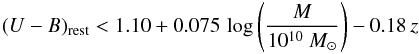
“red-sequence” galaxies. In their analysis, Peng et al. (2010) defined a color-mass relation calibrated on Sloan Digital Sky Survey (SDSS) and zCOSMOS-10k data, dividing red-sequence from blue-cloud galaxies. This relation also takes the redshift evolution into account and is a weak function of mass. Following their approach, 4889 red galaxies were selected on the basis of the following dividing rest-frame (U − B) color.
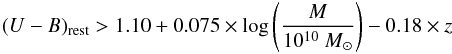
-
“red UVJ” galaxies. Following Williams et al. (2009), we extracted a sample of galaxies on the basis of the restframe color−color diagram defined as
![Mathematical equation: \begin{eqnarray*} (U-V)_{\rm rest}>0.88\times(V-J)_{\rm rest}+0.69\;\;\;[0<z<0.5] \\ (U-V)_{\rm rest}>0.88\times(V-J)_{\rm rest}+0.59\;\;\;[0.5<z<1], \end{eqnarray*}](/articles/aa/full_html/2013/10/aa21797-13/aa21797-13-eq58.png) with the additional constraints of (U − V)rest > 1.3 and (V − J)rest < 1.6. With these cuts, we selected 4882 galaxies.
with the additional constraints of (U − V)rest > 1.3 and (V − J)rest < 1.6. With these cuts, we selected 4882 galaxies. -
“red SED” galaxies. Ilbert et al. (2009) employed a set of templates, generated by Polletta et al. (2007) with the code GRASIL (Silva et al. 1998), to fit the VIMOS VLT Deep Survey (VVDS) sources (Le Fèvre et al. 2005) from the UV-optical to the mid-IR. Therefore, this set of templates provides a better joining of UV and mid-IR than those previously proposed by (Ilbert et al. 2006). The nine galaxy templates of Polletta et al. (2007) include three SEDs of elliptical galaxies and six templates of spiral galaxies (S0, Sa, Sb, Sc, Sd, Sdm). Twelve additional templates obtained from BC03 models with starburst ages ranging from 3 to 0.03 Gyr are also added to better represent the data. Finally, the templates were linearly interpolated, so that a total set of 32 templates was obtained. These templates were used to estimate photometric types from a best fit to the observed photometry without additional dust extinction. With this method, we selected 2603 galaxies best fitted with an early-type template (i.e., SED-type from 1 to 8).
-
“quiescent” galaxies. Following Ilbert et al. (2010) and Pozzetti et al. (2010), we selected 2937 quiescent galaxies on the basis of their sSFR, adopting the cut log (sSFR) < − 2 [Gyr-1]. As shown by Ilbert et al. (2010), this cut corresponds almost directly to a cut (NUV − r+)template > 3.5, with which they defined their sample of quiescent galaxies. With these selection criteria, we select galaxies that are increasing their mass at a rate less than 1/100th of their present mass.
-
“red and passive ETGs”. To obtain a reliable sample with as little bias as possible due to the presence of star-forming contaminants, we decided to follow the approach used in Moresco et al. (2010). From the parent sample, 1530 ETGs were extracted by combining photometric, morphological, and optical spectroscopic criteria: galaxies were chosen with a best fit to the SED matching a local E-S0 template (using the CWW templates of Ilbert et al. 2006), weak/no emission lines (EW0( [OII] /Hα) < 5 Å), spheroidal morphology, and an observed (K − 24 μm) color typical of E/S0 local galaxies (i.e., (K − 24 μm)< − 0.5); for further details about the sample selection, see Moresco et al. (2010).
Other standard definitions involve, for example, different sets of templates to perform a best-fit match to the observed SED (CWW photometric types, Ilbert et al. 2006) or different cuts in the observed colors, as for the case of luminous red galaxies (LRG, Eisenstein et al. 2001) and Baryon Oscillation Spectroscopic Survey (BOSS, Schlegel et al. 2009) samples. We checked, however, that the performances of these criteria are much worse than those of the other samples selected in our analysis in the selection of a pure sample of passive galaxies. In particular, LRGs and BOSS selections were optimized for the specific properties of those surveys and cannot straightforwardly be applied to zCOSMOS survey; we refer to Masters et al. (2011) for a discussion of the contamination by late-type morphological types of BOSS galaxies.
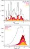 |
Fig. 1 Redshift distribution (upper panel) and stellar mass distribution (lower panel) of the entire zCOSMOS-20k sample and of the different sample. In violet the morphological ETGs, in light red the red-sequence galaxies, in dark red the red UVJ galaxies, in pink the red SED galaxies, in orange the quiescent galaxies, and in yellow the red & passive ETGs. |
Passive galaxy samples overlap depending on the different selection criteria adopted and number of galaxies (in boldface).
In Fig. 1 we show the redshift and mass distribution of the various samples. Each sample was further divided into six subsamples after we considered separately two redshift ranges (z ≤ 0.5 and z > 0.5), three mass ranges (low-mass log (M/M⊙) < 10.25, medium-mass 10.25 ≤ log (M/M⊙) < 10.75, and high-mass log (M/M⊙) ≥ 10.75) in order to be able to discern the dependencies on mass and redshift.
In Table 1 we report the number of galaxies obtained with the different selections, as well as the percentage overlap between the various samples. As expected, the overlap between samples obtained with different selection criteria is often partial, suggesting that they have different properties. In particular, we notice that there is a small overlap between all samples and the morphologically selected sample, indicating that a large fraction of passive galaxies selected on the basis of colors, or more generically on the basis of photometric properties, do not have an E/S0 morphology (see Sect. 3.3). The overlap is also small when considering how many morphologically selected ETGs are found in the other samples, indicating that a non negligible fraction of ellipticals have blue colors. The overlap is, instead, larger when considering the other samples. The red-sequence and red UVJ samples provide an almost identical number of galaxies and show a similar reciprocal overlap of ~80%. However, as we see in the following section, they have different photometric properties. The fraction of galaxies overlapping with the red-sequence sample is above ~80%, irrespective of the selection criterion considered; however this is probably due to the higher number of galaxies of that sample. What is more interesting is to consider the fraction of galaxies included in the quiescent sample: the overlap with the red SED and the red & passive ETGs samples is above ~85%, which testifies a quiescent star-formation activity. However, for the red-sequence and the red UVJ samples, the overlap is ~60%, indicating that almost half of that sample have a higher star-formation activity. The last remark is about the red & passive ETGs criterion, which presents a small overlap with all the other samples: this is partly because of the smaller number of galaxies included in this sample and partly because this is the only sample also comprising a spectroscopic cut (see Sect. 3.2).
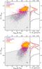 |
Fig. 2 (U − B)rest-mass diagram. In gray is shown the entire zCOSMOS-20k sample, in violet the morphological ETGs, in light red the red-sequence galaxies, in dark red the red UVJ galaxies, in pink the red SED galaxies, in orange the quiescent galaxies, and in yellow the red and passive ETGs. The upper plot shows the (U − B)rest-mass diagram obtained for z ≤ 0.5, and the lower plot shows the diagram obtained for z > 0.5. The gray hatched area represents the region that falls outside the passive region of the (U − B)rest-mass diagram, as defined in Sect. 2.2. The representative errorbar for both quantities is shown in the bottom right corner. |
3. The analysis
As already discussed, the ETGs population is rather homogeneous in color, star-formation activity, and morphology. We therefore decided to inspect in detail different properties to study how their global properties change for the different samples.
3.1. Color properties
The primary observable, apart from the morphology, that we decided to examine, is the color. We decided to study both the standard (U − B)rest color-mass and (U − V)rest − (V − J)rest color−color plots, as well as an IRAC color−color diagram as first introduced by Lacy et al. (2004).
The (U − B)rest-mass diagram is shown for both redshift ranges (z ≤ 0.5 and z > 0.5) in Fig. 2. The gray hatched area represents the region that falls outside what is considered the red sequence, as defined by Peng et al. (2010) and previously reported. The clearest evidence is that most samples lie as expected in the red-sequence region; this is not surprising, since most selection criteria are based (or partially based) on an optical-color selection. For the morphologically selected ETGs, we found a confirmation of what was deduced from Table 1, i.e., that this sample is contaminated by the presence of a non-negligible tail of galaxies with blue (U − B)rest colors (~12−65%), both at high and low redshifts. Quite surprising is the tail of red UVJ galaxies with blue color, which even forms a second peak in the (U − B)rest distribution at z ≤ 0.5 (as shown in Fig. 2). This tail is due to the fact that the cut proposed by Williams et al. (2009) does not perfectly fit the observed bimodality in the UVJ diagram of the zCOSMOS-20k sample.
The (U − V)rest − (V − J)rest diagram provides complementary information with respect to the color-mass diagram. As in the previous plot, we notice that the red & passive ETGs, the quiescent galaxies, and the red SED samples well fit the passive region defined by Williams et al. (2009) and identified by the non-hatched region of Fig. 3; we also observe as before the quite prominent tail of morphological ETGs with quite blue colors. Less expected is the fact that the red-sequence galaxies display a non-negligible fraction of galaxies which do not fit perfectly the passive UVJ region. We will further discuss the issue of the different behavior of red-sequence and red UVJ galaxies in Sect. 4.5.
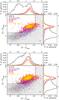 |
Fig. 3 (U − V)rest − (V − J)rest diagram. In gray is shown the entire zCOSMOS-20k sample, in violet the morphological ETGs, in light red the red-sequence galaxies, in dark red the red UVJ galaxies, in pink the red SED galaxies, in orange the quiescent galaxies, and in yellow the red & passive ETGs. The upper plot shows the diagram obtained for z ≤ 0.5, and the lower plot for z > 0.5. The gray hatched area represents the region that falls outside the passive region of the UVJ diagram, as defined in Sect. 2.2. The representative errorbar for both quantities is shown in the bottom right corner. |
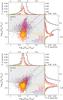 |
Fig. 4 log (S8.0/S4.5) − log (S5.8/S3.6) diagram. In gray is shown the entire zCOSMOS-20k sample, in violet the morphological ETGs, in light red the red-sequence galaxies, in dark red the red UVJ galaxies, in pink the red SED galaxies, in orange the quiescent galaxies, and in yellow the red & passive ETGs. The upper plot shows the log (S8.0/S4.5) − log (S5.8/S3.6) diagram obtained for z ≤ 0.5, and the lower plot shows the diagram obtained for z > 0.5. The gray hatched area represents the region that falls outside the passive region of the IRAC color−color diagram, as defined in Sect. 3.1. The dotted lines represent the region defined by Lacy et al. (2004) to identify AGN candidates, and the dashed lines the revised definition by Donley et al. (2012). The representative errorbar for both quantities is shown in the bottom right corner. |
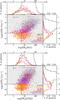 |
Fig. 5 sSFR-EW0( [OII] /Hα) diagram. In gray is shown the entire zCOSMOS-20k sample, in violet the morphological ETGs, in light red the red-sequence galaxies, in dark red the red UVJ galaxies, in pink the red SED galaxies, in orange the quiescent galaxies, and in yellow the red & passive ETGs. The upper plot shows the sSFR-EW0(Hα) diagram obtained for z ≤ 0.5, and the lower plot shows the sSFR-EW0( [OII]) diagram obtained for z > 0.5. The representative errorbar for both quantities is shown in the upper left corner. |
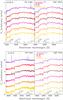 |
Fig. 6 Median stacked spectra obtained for z ≤ 0.5 (upper plot) and z > 0.5 (lower plot); the spectra have been evaluated in the low-mass bin (log (M/M⊙) < 10.25, left panels) and in the high-mass bin (log (M/M⊙) > 10.75, right panels). In violet are shown the morphological ETGs, in light red the red-sequence galaxies, in dark red the red UVJ galaxies, in pink the red SED galaxies, in orange the quiescent galaxies, and in yellow the red and passive ETGs. |
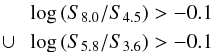
The IRAC observed color−color plot is more interesting since these colors less directly (or not at all) influence the various selection criteria and are therefore a better indication of how much the samples are biased. As defined by Lacy et al. (2004), we plotted the 8.0 μm/4.5 μm ratio against the 5.8 μm/3.6 μm ratio in Fig. 4. This plot was initially introduced to identify active galactic nuclei (AGN) candidates, which should lie in the region identified by the dotted lines. More recently, Donley et al. (2012) revised this selection criterion to reduce the contamination by normal star-forming galaxies by narrowing the region where the AGN candidates should lie (the area identified by the dashed lines). In their work, they also studied the predicted z = 0−3 IRAC colors of different templates as a function of the AGN fraction, considering a star-forming template, a starburst, a normal star-forming spiral galaxy, and an elliptical galaxy. By analyzing the tracks of the elliptical galaxies, we found that they occupy a very specific region of the IRAC color−color diagram, i.e., log (S8.0/S4.5) < − 0.1 ∩ log (S5.8/S3.6) < − 0.1, at least up to z ~ 2; this region is indicated as the non-hatched region of Fig. 4. From this plot, it is evident that in both redshift ranges most of the samples are well located in a clump inside the region just defined; however, different from the color diagrams, there are more pronounced tails outside this region. At z ≤ 0.5 almost all samples show a very significant vertical tail with blue colors in S5.8/S3.6 and red colors in S8.0/S4.5, which is a region in which low-redshift star-forming galaxies lie (for a comparison, see Fig. 2 of Donley et al. 2012). In contrast, for z > 0.5 the tails move toward red colors in both S5.8/S3.6 and S8.0/S4.5. Even if they fall inside the AGN candidate region defined by Lacy et al. (2004), it is very likely that most of these galaxies are higher redshift star-forming galaxies, as can be found following the tracks of Donley et al. (2012).
3.2. Spectroscopic properties
The spectroscopic properties of the galaxies have not been used (except in the red & passive ETGs criterion) to select passive galaxies; therefore, they may provide interesting insights concerning the contamination of the various samples. We decided to look at the restframe equivalent widths (EW0) of [OII] and Hα lines since they are well-known indicators of star-formation activity. Given the wavelength coverage of zCOSMOS spectra, the two lines are not present in both redshift ranges: in particular Hα line is observable at z ≤ 0.5, while [OII] is observable at z > 0.5. These lines will be compared with another indicator of star formation, the sSFR, which provides the relative contribution of the SFR by weighting it with the total stellar mass of the galaxy.
Figure 5 shows log (sSFR/Gyr-1) versus EW0(Hα) (upper panel; z > 0.5) and EW0( [OII]) (lower panel; z ≤ 0.5). As expected, there exists a correlation (even if with a large dispersion) between the sSFR and the equivalent widths of [OII] and Hα emission lines. Ilbert et al. (2010), aiming to study the galaxy stellar mass assembly by morphological and spectral type in the COSMOS field, identified as quiescent galaxies those with a dereddened color (NUV − r+) > 3.5 and consequently having log (sSFR/Gyr-1) < − 2. Mignoli et al. (2009), analyzing the zCOSMOS sample, found that strong and weak line emitters can be well divided by an EW0( [OII] ) = 5 Å. Combining this information, we therefore identified log (sSFR/Gyr-1) < − 2 ∩ EW0(Hαor [OII] ) < 5 Å as the region characteristic of quiescent galaxies in this plot (the non-dashed area).
The quiescent galaxies and the red & passive ETGs samples present, by definition, no tail at high sSFR and EWs, respectively. From the plot, we find that the color-selected samples (red UVJ and red-sequence) and the morphological selected sample instead display a marked percentage of galaxies placed at both high sSFR and EWs, both at low and high redshifts. While the interpretation of intermediate values of emission lines in terms of star formation (see for example Yan et al. 2006; Yan & Blanton 2012) is not straightforward, especially in the presence of a low level of sSFR, the concomitant higher level of sSFR clearly indicates a higher level of star formation with respect to the bulk of the population, which lies in the passive region defined above.
We have also analyzed the stacked median spectra of all samples. In order to disentangle mass and redshift effects, in Fig. 6 we plotted only the median spectra for the low- (log (M/M⊙) < 10.25) and high-mass (log (M/M⊙) > 10.75) subsamples, in the low- and high-redshift regimes. At both high and low redshift, several emission lines are clearly detectable for most samples. However, one of the most striking result is that emission lines disappear when passing from the low-mass to the high-mass regime. This represents noticeable evidence that this population is more quenched than the other. We further inspect this trend in Sect. 4.2.
The morphological ETGs present the strongest emission lines, especially at low masses. At high redshift, strong emission lines in [OII], Hβ, and [OIII] are found. At low redshift, the measured ratios between [NII]λ6583/Hα and [OIII]λ5007/Hβ populate the star-forming region in the BPT diagram (Baldwin et al. 1981). This indicates a significant star formation, in particular if we consider that we are analyzing median spectra (see also Pozzetti et al. 2010).
All the other samples show spectra with more typical passive continua, with the presence of faint emission lines in [OII] and Hα only for the red UVJ and red-sequence galaxy samples. At high masses, we find no traces of significant emission lines, and all the spectra show features and continua typical of passively evolving galaxies; this indicates a possible mass dependence that will be further analyzed in Sect. 4.2. In particular, we notice small [OII] emission lines in most spectra at high redshifts, which, however, is compatible with not being caused by star-formation activity (see Yan et al. 2006; Yan & Blanton 2012, and the discussion of Sect. 4.1). At low redshift, we note that all spectra present a detectable [NII] line (and often also [SII]), but no sign of Hα, probably due to the fact that the Hα emission line is hidden by the corresponding absorption line.
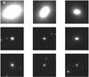 |
Fig. 7 Examples of ACS morphology for a subsample of the red and passive ETGs with elliptical morphologies. The galaxies are shown at increasing redshift from upper left to lower right, from z = 0.0791 to z = 0.9302. |
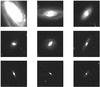 |
Fig. 8 Examples of ACS morphology for a subsample of the red & passive ETGs with very late-type morphologies, found for less than 10% of the overall sample. The galaxies are shown at increasing redshift from upper left to lower right, from z = 0.0998 to z = 0.834. |
3.3. Morphological properties
To study in detail the morphological properties, we analyzed the ZEST (Scarlata et al. 2007a) types of the various samples. While for almost all the samples a large fraction of galaxies have an E/S0 morphology (a clear example is shown in Fig. 7), there is a significant fraction, which depends on the adopted selection criteria, of galaxies with clearly spiral/irregular morphologies (see Fig. 8). Despite the evident correspondence between the bimodality in photometric properties and in morphological types, all the samples are contaminated by late-type morphologies: this suggests that the color and the morphological transformation are two distinct processes taking place at different times in the life of a galaxies.
This result confirms what was found with independent methods by other analyses (see, for example, Pozzetti et al. 2010; Ilbert et al. 2010), i.e., that the morphological transformation from late-type to early-type galaxies is a process which intervenes on different timescales than the color transformation. As a result, it is likely for a galaxy, even if it has already stopped its star-formation activity, not to have an elliptical morphology. In contrast to other properties, it is thus improper to consider those galaxies as star-forming contaminants, and the presence of morphologically late-type galaxies will be considered separately.
Contamination of the different samples of passive galaxies as a function of stellar mass and redshift.
4. Results
To quantitatively estimate which is the best (i.e., the least biased as possible) selection criterion, we estimated the level of contamination by examining different observables, considering colors, sSFR, spectroscopic features, and visual morphology. Of course, as anticipated, these criteria should not to be too restrictive because otherwise we trade purity for a poor completeness.
By definition, the less contaminated criterion will be the red & passive ETGs since it uses all the possible information available for these galaxies. However, in the context of many galaxy surveys, it is of utmost interest to also identify a sample that is at the same time the most economic as possible (in terms of information used) and as less biased as possible (in terms of star-forming outliers). To carry on this analysis, it is necessary not only to consider the percentage of contaminants present in each sample but also their absolute values, as well as the dependence on the redshift and on the stellar mass of the contamination.
4.1. Study of the contamination
The criteria adopted to define a contaminant are complementary to the ones used to select the various samples of passive galaxies and are described as:
-
blue (U − B)rest colors:
-
nonpassive UVJ colors:
![Mathematical equation: \begin{eqnarray*} (U-V)_{\rm rest} &<& 0.88\times(V-J)_{\rm rest}+0.69\; \\&&\times{[+0.59\;\;{\rm for}\;\;z>0.5]} \\ \cup\;\;(U-V)_{\rm rest} &<& 1.3\;\;\cup\;\; (V-J)_{\rm rest}>1.6 \end{eqnarray*}](/articles/aa/full_html/2013/10/aa21797-13/aa21797-13-eq102.png)
-
nonpassive IRAC colors:
-
high sSFR:
![Mathematical equation: \begin{eqnarray*} \log\,({\rm s}{\it SFR})>-2\;[{\rm Gyr}^{-1}] \end{eqnarray*}](/articles/aa/full_html/2013/10/aa21797-13/aa21797-13-eq104.png)
-
presence of emission lines:
![Mathematical equation: \begin{eqnarray*} EW_{0}({\rm H}\alpha)>5 ~{\AA}\, ({\rm if} \, z\leq0.5 )\\ {\rm or} \quad EW_{0}([{\rm OII}])>5 ~{\AA} \, ({\rm if} \, z>0.5 ) \end{eqnarray*}](/articles/aa/full_html/2013/10/aa21797-13/aa21797-13-eq105.png)
-
nonelliptical morphology: ZEST type later than E/S0.
For each mass and redshift subsample of the various samples defined in Sect. 2.2, we estimated the median (U − B)rest color, sSFR, IRAC colors, restframe equivalent width of Hα ([OII] for z > 0.5), and morphology of the just defined contaminant, as well as the percentage of contamination relative to each subsample. These values are reported in Table 2.
As discussed above for the morphology, the spectroscopic properties would also be worth a dedicated discussion, since it is not straightforward that a weak [OII] or Hα emission line is symptomatic of star-formation activity (Yan et al. 2006; Yan & Blanton 2012). However, for simplicity we address as a contaminant a galaxy having any of these properties considered non-standard for an early type and examine each one individually.
For each considered property, a trend with stellar mass is evident for all the samples, with a decreasing percentage of contaminants with increasing mass. This effect will be analyzed in the following section. Below we discuss separately the contamination in optical and IRAC colors, in sSFR, in spectroscopy, and in morphology.
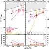 |
Fig. 9 Median (U − B)rest color (upper panel) and relative percentage (lower panel) as a function of stellar mass of galaxies with blue colors, i.e., |

Blue (U − B)rest colors.
In Sect. 3.1 we have shown the (U − B)rest-mass diagram for all the samples, proving that, given the adopted selection criteria, almost all the selected galaxies lie in the red sequence, with minor tails extending in the blue cloud. As a consequence, the number of outliers with clearly blue colors are a minor percentage, typically ≲5% for all criteria (except morphological and red UVJ galaxies) at both low and high redshift. Moreover, as can be inferred from Table 2, this small fraction of blue outliers has relatively red colors, very close to the considered separation between red sequence and blue cloud. In contrast, morphological ETGs display a substantial percentage of galaxies, ~12−65% depending on the redshift range and on the mass regime, with a median (U − B)rest color bluer with respect to the contaminants present in the other samples. This fact testifies that even if a correlation exists between photometric properties and morphology of passive galaxies, it is not a one-to-one correlation, and a considerable number of blue ellipticals coexist with their more standard red counterparts (see also Tasca et al. 2009). Also the red UVJ sample presents a significant contamination, ~30−10% depending on the redshift range and on the mass regime. This is probably due to the fact that the color cuts defined by Williams et al. (2009) do not seem to reproduce well the observed bimodality in the UVJ diagram (as it can be seen by Fig. 3), with tails evident in the blue part of the (U − V)rest histogram. However, the median color of the contaminant is, as in most of the previous cases, very close to the adopted definition of red sequence. All these data are reported in Table 2 and shown in Fig. 9.
Nonpassive UVJ colors.
For the UVJ color−color diagram, we considered as a contaminant a galaxy with (U − V)rest and (V − J)rest colors outside the region defined by Williams et al. (2009). Therefore we just estimated the percentage of these galaxies for each selection criterion; we refer to Sect. 3.1 for the discussion about where those contaminants lie in the UVJ color−color diagram.
This analysis confirms the results just discussed for the color-mass diagram: the quiescent galaxies, red SED galaxies, and red & passive ETGs fit almost perfectly to the passive region in the UVJ diagram, with a percentage of contaminants always below 20% at low redshift and below 5% at high redshift. The percentage of contaminants is slightly higher for the red-sequence sample, around 10−30%, and this fact demonstrates that the cut defined by Peng et al. (2010) in the (U − B)rest is also not optimal in dividing passive and star-forming galaxies. As in the previous analysis, the morphological ETGs are the sample with the highest contamination in UVJ colors, around 12−65% depending on the redshift and mass ranges.
Nonpassive IRAC colors.
The study of the IRAC colors allows a clearer estimate of the presence of star-forming contaminants since these bands were not directly used to define ETG samples (they were used in the red SED galaxies, but together with all the other photometric bands for the best fit to the SEDs). We considered as a contaminant a galaxy falling outside the passive IRAC selection defined in Sect. 3.1. Therefore, since it is possible for such galaxy to have a redder S5.8/S3.6 color or a redder S8.0/S4.5 color, or both, as for the UVJ case, we just estimated the percentage of these galaxies for each selection criterion and refer to Sect. 3.1 for the discussion about where those contaminants lie in the IRAC color−color diagram.
The morphological ETGs are the sample with the higher percentage of contamination, ~20−75% depending on the mass and redshift range. Similar to the case of the sSFR, the red UVJ and the red-sequence galaxies are more biased, with ~25−55% (depending on the mass range) of the sample not classified as passive for the IRAC color−color criterion at z ≤ 0.5 and ~10−50% at z > 0.5. Apart from the red & passive ETGs sample, with a contamination of ~5−25% at low redshift and of ~2−40% at high redshift (from the lowest to the highest masses), the purest samples are the quiescent and the red SED galaxies (~10−45% at low redshift and ~3−45% at high redshift).
High sSFR.
Considering the sSFR, the morphological ETGs are the sample with the most extended tails (~30−90%), with median values up to log (sSFR/Gyr-1) ~ − 0.6, corresponding to a star-formation activity ~25 times higher with respect to the adopted definition of quiescent (i.e., log (sSFR/Gyr-1) < − 2). Both red UVJ and red-sequence samples represent an intermediate case, with a median log (sSFR/Gyr-1) ~ − 1.5/−1.7 for the contaminants (~3 times more star-formation activity than the assumed quiescent limit), and a percentage of contamination ~20−65%, depending on the mass range. The less biased samples (the quiescent sample is by definition not biased with respect to this parameter) are the red SED and the red & passive ETGs ones, having median values of sSFR much closer to the quiescent limit and a percentage of contamination in most cases ≲15%. All these data are reported in Table 2 and shown in Fig. 10.
Presence of emission lines.
We estimated the median equivalent width of Hα at z ≤ 0.5, and [OII] at z > 0.5 for the galaxies with significant emission lines (i.e., >5 Å) in each sample; the results are reported in Table 2 and shown in Fig. 11. The sample with the strongest emission lines is the morphological ETGs, with median equivalent widths up to ~30 Å and with a percentage of contamination going from 55−70% to 35%, depending on the mass range. The red UVJ and the red-sequence samples show a similar and smaller contamination, both in percentage (~40%) and median value (~15−10 Å). The less contaminated samples are the quiescent and the red SED galaxies: the percentage of galaxies with emission lines >5 Å is ~30% at low redshift and slightly smaller (~20%) at higher redshift, with median values closer to the adopted cut (~8−10 Å).
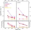 |
Fig. 10 Median log (sSFR/Gyr-1) (upper panel) and relative percentage (lower panel) as a function of stellar mass of galaxies with high sSFR, i.e., log (sSFR/Gyr-1) > −2, for the different selection criteria (in violet the morphological ETGs, in light red the red-sequence galaxies, in dark red the red UVJ galaxies, in pink the red SED galaxies, in orange the quiescent galaxies, and in yellow the red & passive ETGs). The errorbars represent the error on the median. |
Many works have already shown the presence of emission lines in the spectra of red/passive galaxies. However, given their line ratios, these are usually classified as LINERS (low-ionization nuclear emission-line regions, Heckman 1980), or with a LINER-like emission (e.g., see Phillips et al. 1986; Yan et al. 2006; Annibali et al. 2010; Yan & Blanton 2012). As summarized by Annibali et al. (2010), the most probable mechanisms proposed to produce such lines are a low accretion-rate AGN, fast shocks, or photoionization by old post-asymptotic giant branch (PAGB) stars. More recent studies favor the last option (see also Yan & Blanton 2012). It is beyond the aim of this paper to analyze in detail the source of ionization in this population of galaxies; what we wanted to stress here is that in this population of galaxies weak emission lines do not necessarily trace star-formation activity, especially if the sSFR as found from the SED-fitting does not confirm a significant star formation. On the other hand, the stronger emission lines found in morphological ETGs should actually trace star-formation activity, as confirmed by the ratio with the other significant emission lines (Hβ, [NII]λ6583, [OII]λ5007).
Nonelliptical morphology.
The median morphology estimated for the galaxies not matching an elliptical template is equal to a ZEST type =2.1 in all samples, which corresponds to a bulge-dominated spiral galaxy. This means that for all samples the tail of morphologies is not extended toward very late-type templates. However, all the samples show a high percentage of contamination due to non elliptical-galaxies, with percentages going from ~60% at low masses to ~25−30% at high masses, the less biased sample being the red & passive ETGs one.
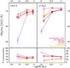 |
Fig. 11 Median EW0(Hα) (upper panel; EW0( [OII]) if z > 0.5) and relative percentage (lower panel) as a function of stellar mass of galaxies with significant emission lines, i.e., EW0(Hα) > 5 Å (if z ≤ 0.5) and EW0( [OII] ) > 5 Å (if z > 0.5), for the different selection criteria (in violet the morphological ETGs, in light red the red-sequence galaxies, in dark red the red UVJ galaxies, in pink the red SED galaxies, in orange the quiescent galaxies, and in yellow the red & passive ETGs). The errorbars represent the error on the median. By convention, the emission lines are quoted with negative values. |
This evidence confirms that the color transformation and the morphological transformation from late-type to early-type galaxies are not concomitant processes and that the quenching of the star-formation activity could precede the change in morphological type.
4.2. Contamination as a function of mass
The analysis of the different properties of passive galaxies indicated a clearly evident dependence of the contamination on the stellar mass. Looking at Table 2, it is possible to see that the percentage of contamination in almost all the analyzed properties decreases from log (M/M⊙) < 10.25 to log (M/M⊙) > 10.75 by a factor ~2−3. Figures 9, 10, and 11 also highlight a mass dependence of the absolute value of the properties of the contaminants in all samples: for example the colors of contaminants are redder by ~10−30% at high masses than at low masses and are closer to the red sequence. This trend can also be found in sSFR and equivalent widths of emission lines, with the lower mass bin having a star-formation activity ~10% higher and emission lines ~5 Å larger than the high-mass bin for all the samples considered, both at high and at low redshift.
From this analysis we found that, irrespective of the adopted selection criterion, an additional stellar mass cut provides a purer sample of passively evolving galaxies, significantly reducing the contamination by star-forming galaxies.
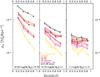 |
Fig. 12 Redshift evolution of the galaxy number density, derived using 1/Vmax, for three different mass ranges: 10.25 < log (M/M⊙) < 10.75 (left panel), 10.75 < log (M/M⊙) < 11 (central panel) and log (M/M⊙) > 11 (right panel). The different colors represent different selection criteria (violet for the morphological ETGs, light red for the red-sequence galaxies, dark red for the red UVJ galaxies, pink for the red SED galaxies, orange for the quiescent galaxies, and yellow for the red & passive ETGs). The lines represent the fit to the observed log (ρN(z)) relation. The open points represent the lower limits where the survey is not complete. |
4.3. Contamination as a function of selection criteria
There are different ways to quantify the best method to select a population of passively evolving galaxies. On one hand, it is possible to ask which criterion is least biased by the presence of star-forming outliers, independently of how much information is used. On the other hand, at a fixed percentage of contamination, it is possible to ask which is the most economic criterion in terms of information used. The first will privilege the purity of the sample but has the drawback of requiring a large amount of data to be used. In contrast, the second will be necessarily more contaminated but also of greatest interest in many surveys where less data are available, due to low spectral resolution or limited wavelength coverage.
Needless to say, the purest sample is the one based on the combined selection criterion since the use of photometric, spectroscopic, and morphological information helps to minimize the presence of blue, star-forming galaxies. It provides red and passive galaxies with a color contamination, also in the IRAC colors, <10% for stellar masses log (M/M⊙) > 10.25, both at low and high redshifts. The specific star formation of the outliers (≲10% for log (M/M⊙) > 10.25) is only ~20% higher than the chosen passive cut, and the contaminants equivalent widths of emission lines, both [OII] and Hα, are smaller than ~10 Å.
Apart from this criterion, all the others, except the morphological criterion, are equivalent in terms of requirements since they all need a best fit to the observed SED to obtain stellar masses, SFRs, and/or restframe colors necessary to perform the selection. Among them, the best-performing criteria have proven to be the red SED and the quiescent ones. An analysis of Table 2 and Figs. 9−11 shows that they have the minimum percentage of contamination in both optical colors (≲5%), IRAC colors (≲15%), spectroscopic features (≲30%), and sSFR (≲15%). The percentage of contamination is slightly higher than the red & passive ETGs criterion, on average by a factor of ~2, but the absolute values of the properties of contaminants are still compatible with a red, passively evolving population.
4.4. Number density
For all the samples, we estimated the galaxy stellar mass functions using the nonparametric 1/Vmax formalism (Schmidt 1968), from which we derived the number density (ρN) in three mass bins, log (M/M⊙) = 10.25−10.75,10.75−11,11−11.5. The redshift evolution of the galaxy number density is shown in Fig. 12. As a comparison, we also reported the number density in the same mass range for the parent zCOSMOS-20k sample. Each relation was fitted using a weighted linear least square minimization, considering only the redshift bins in which the data are complete. The trends are similar for the differently selected samples, even if the normalization is different.
In the lower stellar mass bin, we find a pronounced evolution, with an increase in number densities by a factor ~2−4 between z ~ 0.65 and z ~ 0.2. At stellar masses 10.75 < log (M/M⊙) < 11, we still find a noticeable evolution, with an increase by a factor ~2−3 between z ~ 0.85 and z ~ 0.2. At higher masses, 11 < log (M/M⊙) < 11.5, the evolution is much less pronounced, with a percentage increase in number density of ~10−50% in the entire redshift range.
The stronger increase in the number density of low/intermediate-mass passive galaxies with respect to massive and passive galaxies is a clear indication of mass-assembly “downsizing” (Fontana et al. 2004; Drory et al. 2005; Bundy et al. 2006; Cimatti et al. 2006; Thomas et al. 2010; Pozzetti et al. 2010; Moresco et al. 2010), with more massive galaxies having assembled their mass at higher redshifts and already being in place at z ~ 1. The result of this analysis is in agreement with many other works: Scarlata et al. (2007b) studying ETGs in the COSMOS field found no traces of significant evolution in the number density of bright (~L > 2.5L∗) ETGs, with a maximum increase of ~30% from z ~ 0.7 to z ~ 0 when allowing for different SFHs and cosmic variance; Pozzetti et al. (2010) found an almost negligible evolution in the number density of quiescent galaxies in zCOSMOS-10k sample, <0.1 dex between z = 0.85 and z = 0.25 for log (M/M⊙) > 11−11.5; from the analysis of the UltraVISTA-DR1 sample Ilbert et al. (2013) found that massive galaxies (log (M/M⊙) > 11.2) do not show any significant evolution between 0.8 < z < 1.1 and 0.2 < z < 0.5, while low-mass ones (log (M/M⊙) ~ 9.5) increase in number density by a factor >5. Brammer et al. (2011) analyzed the number density of quiescent galaxies at 0.4 < z < 2.2 using the NEWFIRM Medium-Band Survey, and found a strong evolution of log (M/M⊙) > 10.5 galaxies, a factor ~10 from z ~ 2 to z ~ 0. However, this evolution becomes smaller and comparable with the errorbars at high masses between z ~ 1 and z ~ 0.6, only ~20% for log (M/M⊙) > 11 (~10% for 10.6 < log (M/M⊙) < 11), therefore it is compatible with our results. Maraston et al. (2012), studying the stellar mass function of BOSS galaxies, find that the galaxy number density above ~2.5 × 10¹¹ M⊙ agrees with previous measurements within 2σ, with no evolution detected from z ~ 0.6. Also from the analysis of the VIPERS survey, Davidzon et al. (2013) find a much stronger evolution in the number density of less massive galaxies when compared to less massive ones, with an increase of ~80% between z = 1 and z = 0.6 for masses 11 < log (M/M⊙) < 11.4 and only of ~45% between z = 1.2 and z = 0.6 for masses log (M/M⊙) > 11.4. Finally, Moustakas et al. (2013) measured the evolution of the stellar mass function from the PRism MUlti-object Survey and confirmed an evolution by a factor of 3.2 ± 0.5 from z = 0.4 to z = 0 for stellar masses 9.5 < log (M/M⊙) < 10, by a factor of 2.2 ± 0.4 from z = 0.6 to z = 0 for stellar masses 10 < log (M/M⊙) < 10.5, and only ~58% ± 9% for stellar masses 10.5 < log (M/M⊙) < 11.
The comparison, at fixed mass, of the number density of the differently selected passive galaxies is also interesting since it sheds some light on the timescales characteristic of different processes. At masses log (M/M⊙) < 11, we find that the number densities of the various samples are well separated, with highest normalization for color-selected ETGs, intermediate for the passive/red-SED/morphologically selected ETGs, and lowest for the red & passive ETGs. This may suggest a scenario during which, at these masses, the first transition that an ETG experiences is a color transformation from blue to red, followed by the quenching of the star formation and by the morphological transformation into ellipticals.
A similar trend is found in the work of Pozzetti et al. (2010), which quantified the timescale of the delay between color and morphological transformation to be around 1−2 Gyr. Some support to this scenario also comes from the work of Ilbert et al. (2010), who find that the stellar mass density of quiescent galaxies is always higher than the one of red elliptical galaxies. Obviously the quantitative estimate of the delay between these processes also depends on the adopted cuts to select ETGs since, for example, a lower/higher cut in sSFR will shift the relation lower/higher.
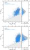 |
Fig. 13 (U − B)rest-mass diagram. In gray is shown the original (U − B)rest-mass criterion as defined by Peng et al. (2010), and in cyan are highlighted the galaxies presenting a sSFR or emission lines in excess with respect to the passive cuts. The empty cyan histograms show the distribution of the contaminants with the old definitions, while the shaded cyan histograms show the distribution of the contaminants with the new selection criterion as defined in Sect. 4.5. The upper plot shows the diagram obtained for z ≤ 0.5, and the lower plot shows the diagram obtained for z > 0.5. |
4.5. Revising the color selection criteria
In Sects. 3.1 and 4.1 we presented and discussed the fact that the red-sequence and the red UVJ samples have a higher contamination, which is also clearly evident by a visual inspection of the color-mass and color−color diagrams. However, we also argued that this higher contamination may be due to the fact that the proposed cut may not be optimal, at least for the zCOSMOS-20k survey.
To address this issue, we decided to study how the colors of the contaminants (as defined in Sect. 4.1) for these two criteria are distributed in the (U − B)rest color-mass and UVJ color−color diagrams, respectively, in order to understand if an additional cut is able to further reduce the contamination. In Fig. 13 we show the (U − B)rest-mass diagram for the red-sequence galaxies (in gray), highlighting in cyan the galaxies presenting a sSFR or emission lines in excess with respect to the passive cuts defined (i.e., the contaminants); Fig. 14 shows the same as Fig. 13, but for the (U − V)rest − (V − J)rest diagram and for the case of the red UVJ galaxies. From these plots it is evident that statistically the contaminants have bluer colors and therefore that a refined cut may help to reduce the contamination. In particular from Fig. 14 it is clear that there are specific ranges of colors (1.3 < (U − V)rest < 1.5) where the contaminants represent 100% of the distribution.
We therefore defined two revised color selection criteria, with slightly redder colors: for the (U − B)rest-mass diagram:  and for the (U − V)rest-(V − J)rest diagram:
 ![Mathematical equation: \begin{eqnarray*} \left\{ \begin{array}{ll} (U-V)_{\rm rest}>1.6 &\\ (V-J)_{\rm rest}>1.6 & [0<z<0.5]\\ (U-V)_{\rm rest}>0.88*(V-J)_{\rm rest}+0.69\nonumber \end{array} \right. \\ \left\{ \begin{array}{ll} (U-V)_{\rm rest}>1.5 &\\ (V-J)_{\rm rest}>1.6 & [0.5<z<1]\\ (U-V)_{\rm rest}>0.88*(V-J)_{\rm rest}+0.66.\nonumber \end{array} \right. \end{eqnarray*}](/articles/aa/full_html/2013/10/aa21797-13/aa21797-13-eq172.png) The empty colored histograms in Figs. 13 and 14 show the distribution of the contaminants with the old definitions, while the shaded colored histograms show the distribution of the contaminants obtained with the new definitions just reported. It is evident how these new color selection criteria help to cut significantly the contaminants with blue colors.
The empty colored histograms in Figs. 13 and 14 show the distribution of the contaminants with the old definitions, while the shaded colored histograms show the distribution of the contaminants obtained with the new definitions just reported. It is evident how these new color selection criteria help to cut significantly the contaminants with blue colors.
We checked that these new selection criteria provide purer samples than the previous ones. The new red UVJ sample no longer presents significant blue tails in the color-mass diagram, having a contamination compatible with all the other samples. In addition, the percentage of contamination of the new red-sequence sample in the UVJ color−color diagram is reduced from 20−40% to 15−25% at low redshift and from 20−40% to 10−15% at high redshift. However, even if reduced with these new definitions, the contamination in terms of sSFR and presence of emission lines is still higher than the quiescent, red SED, and red & passive ETGs criteria, which continue to behave better than the color criteria in selecting a purer sample of ETGs.
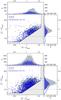 |
Fig. 14 (U − V)rest − (V − J)rest diagram. In gray is shown the original UVJ criterion, as defined by Williams et al. (2009), and in blue are highlighted the galaxies presenting a sSFR or emission lines in excess with respect to the passive cuts. The empty blue histograms show the distribution of the contaminants with the old definitions, while the shaded blue histograms show the distribution of the contaminants with the new selection criterion as defined in Sect. 4.5. The upper plot shows the diagram obtained for z ≤ 0.5, and the lower plot shows the diagram obtained for z > 0.5. |
5. Summary and conclusions
We have studied the photometric, spectroscopic and morphological properties of six differently selected samples of passive galaxies in order to analyze their contamination in terms of blue/star-forming/nonpassive galaxies. From the zCOSMOS-20k spectroscopic catalog, we extracted a sample based on morphology (3336 “morphological” early-type galaxies), on optical colors (4889 “red-sequence” and 4882 “red UVJ” galaxies), on specific star-formation rate (2937 “quiescent” galaxies), on a best fit to the observed SED (2603 “red SED” galaxies), and on a criterion that combines morphological, spectroscopic, and photometric information (1530 “red & passive early-type galaxies”).
For all the samples, we estimated the (U − B)rest-stellar mass diagram, the IRAC color−color plot as defined by Lacy et al. (2004), the sSFR-EW0( [OII] /Hα) diagram, and the morphological types. We also evaluated the median stacked spectra of these samples to search in detail for the presence of peculiar spectroscopic features that may be a proxy of star-formation activity.
To quantify the contamination of the various samples, for each property we defined a passive cut and studied the percentage of galaxies not fulfilling this cut, as well as the median value of the parameters (color, sSFR, EW0 of emission lines) involved in each selection. In this way we were also able to study how much these contaminants are close to or far from the assumed passive definition. All these analyses were performed in two redshift bins (z ≤ 0.5 and z > 0.5) and three stellar mass bins (log (M/M⊙) < 10.25, 10.25 < log (M/M⊙) < 10.75, and log (M/M⊙) > 10.75).
Our main results are listed below:
-
We find that all samples display tails in the star-forming regions ofdifferent diagrams, irrespective of the severity of the criterionadopted. This contamination has been shown to be dependent onthe stellar mass for all the samples, with more massive samplesbeing less biased than less massive ones. This fact demonstratesthat a cut in stellar mass is helpful to improve the purity of thesample.
-
The comparison between the different selection criteria shows that the best performing one is based on a combined selection since it takes into account all the available information about the galaxies (morphological, spectroscopic and photometric), with the obvious disadvantage of being highly demanding in terms of the data needed. For this sample, we find that the contamination is minimized, especially for stellar masses log (M/M⊙) > 10.25: <10% for both optical and IRAC colors, ≲10% in sSFR and with weak emission line equivalent widths for the contaminants (≲10 Å).
-
The morphological criterion is the one with the larger contamination, and a high percentage of blue, emission-line, star-forming elliptical galaxies has been found in this sample (~12−65%, depending on the mass range). Among the other selection criteria, we identify the red SED and the quiescent as the best since their slight increase in contamination (about a factor 2) is offset by the fact that they are extremely economical in terms of information required.
-
The slope of the number density as a function of redshift at fixed mass for the various samples is similar. We found an increase in number density in the mass range 10.25 < log (M/M⊙) < 10.75 from z = 0.65 to z = 0.2 by a factor ~2−4, in the mass range 10.75 < log (M/M⊙) < 11 from z = 1 to z = 0.2 by a factor ~2−3, while for massive ETGs 11 < log (M/M⊙) < 11.5 this increase from z = 1 to z = 0.2 is only ~10−50% (and <10% between z = 1 and z = 0.4). This trend in mass confirms that most massive ETGs are already in place at z ~ 1. The comparison of the different number densities suggests a scenario for ETGs in which the color transformation from blue to red precedes the quenching of the star formation and the morphological transformation from late type to ellipticals.
-
By analyzing the color-mass and color−color diagrams, we proposed two revised selection criteria, which help to reduce the contamination by blue star-forming galaxies.
Selecting a sample of passive galaxies that is as uncontaminated as possible by star-forming objects is crucial for an unbiased study of the properties of this population of galaxies. The analysis presented in this paper provides a first detailed comparison of the contamination obtained with different selection criteria, and represents an important step forward in the identification of the best ways of selecting passive galaxies. This will be especially fundamental for the new and upcoming surveys such as BOSS (Schlegel et al. 2009) and Euclid (Laureijs et al. 2011), which will provide the scientific community unprecedented statistics of these objects, in particular at high redshift. From this point of view, this work represents the starting point to study and develop optimized passive galaxy selection criteria also at z > 1, which could be applied, for example, to Euclid simulations.
In a forthcoming paper we aim to study how much the different selections presented here affect the study of the evolution of passive galaxies.
Acknowledgments
M.M. and A.C. acknowledge the grants ASI n.I/023/12/0 “Attivitá relative alla fase B2/C per la missione Euclid” and MIUR PRIN 2010-2011 “The dark Universe and the cosmic evolution of baryons: from current surveys to Euclid”. Part of the work has also been supported by an INAF grant “PRIN-2010”. This analysis is based on zCOSMOS observations, carried out using the Very Large Telescope at the ESO Paranal Observatory under Programme ID: LP175.A-0839. We would like to thank the anonymous referee for the useful comments and suggestions, which helped to improve the paper.
References
- Annibali, F., Bressan, A., Rampazzo, R., et al. 2010, A&A, 519, A40 [NASA ADS] [CrossRef] [EDP Sciences] [Google Scholar]
- Aviles, A., Bravetti, A., Capozziello, S., et al. 2013, PhRvD, 87, 044012 [NASA ADS] [Google Scholar]
- Baldry, I. K., Glazebrook, K., Brinkmann, J., et al. 2004a, ApJ, 600, 681 [NASA ADS] [CrossRef] [Google Scholar]
- Baldry, I. K., Balogh, M. L., Bower, R., et al. 2004b, AIPC, 743, 106 [Google Scholar]
- Baldry, I. K., Balogh, M. L., Bower, R. G., et al. 2006, MNRAS, 373, 469 [NASA ADS] [CrossRef] [Google Scholar]
- Baldry, I. K., Glazebrook, K., & Driver, S. P. 2008, MNRAS, 388, 945 [NASA ADS] [Google Scholar]
- Baldwin, J. A., Phillips, M. M., & Terlevich, R. 1981, PASP, 93, 5 [NASA ADS] [CrossRef] [EDP Sciences] [Google Scholar]
- Balogh, M., Eke, V., Miller, C., et al. 2004, MNRAS, 348, 1355 [Google Scholar]
- Bell, E. F., Wolf, C., Meisenheimer, K., et al. 2004, ApJ, 608, 752 [NASA ADS] [CrossRef] [Google Scholar]
- Brammer, G. B., Whitaker, K. E., van Dokkum, P. G., et al. 2011, ApJ, 739, 24 [NASA ADS] [CrossRef] [Google Scholar]
- Brinchmann, J., Charlot, S., White, S. D. M., et al. 2004, MNRAS, 351, 1151 [NASA ADS] [CrossRef] [Google Scholar]
- Bruzual, G., & Charlot, S. 2003, MNRAS, 344, 1000 [NASA ADS] [CrossRef] [Google Scholar]
- Bundy, K., Ellis, R. S., Conselice, C. J., et al. 2006, ApJ, 651, 120 [NASA ADS] [CrossRef] [Google Scholar]
- Calzetti, D., Armus, L., Bohlin, R. C., et al. 2000, ApJ, 533, 682 [NASA ADS] [CrossRef] [Google Scholar]
- Capak, P., Aussel, H., Ajiki, M., et al. 2007, ApJS, 172, 99 [NASA ADS] [CrossRef] [Google Scholar]
- Chabrier, G. 2003, PASP, 115, 763 [NASA ADS] [CrossRef] [Google Scholar]
- Cimatti, A., Daddi, E., & Renzini, A. 2006, A&A, 453, L29 [NASA ADS] [CrossRef] [EDP Sciences] [Google Scholar]
- Coleman, G. D., Wu, C.-C., & Weedman, D. W. 1980, ApJS, 43, 393 [NASA ADS] [CrossRef] [Google Scholar]
- Davidzon, I., Bolzonella, M., Coupon, J., et al. 2013, A&A, 558, A23 [NASA ADS] [CrossRef] [EDP Sciences] [Google Scholar]
- Donley, J. L., Koekemoer, A. M., Brusa, M., et al. 2012, ApJ, 748, 142 [NASA ADS] [CrossRef] [Google Scholar]
- Drory, N., Salvato, M., Gabasch, A., et al. 2005, ApJ, 619, L131 [NASA ADS] [CrossRef] [Google Scholar]
- Eisenstein, D. J., Annis, J., Gunn, J. E., et al. 2001, AJ, 122, 2267 [NASA ADS] [CrossRef] [Google Scholar]
- Fontana, A., Pozzetti, L., Donnarumma, I., et al. 2004, A&A, 424, 23 [NASA ADS] [CrossRef] [EDP Sciences] [Google Scholar]
- Franzetti, P., Scodeggio, M., Garilli, B., et al. 2007, A&A, 465, 711 [NASA ADS] [CrossRef] [EDP Sciences] [Google Scholar]
- Garilli, B., Fumana, M., Franzetti, P., et al. 2010, PASP, 122, 827 [NASA ADS] [CrossRef] [Google Scholar]
- Heckman, T. M. 1980, A&A, 87, 152 [NASA ADS] [Google Scholar]
- Hogg, D. W., Blanton, M., Strateva, I., et al. 2002, AJ, 124, 646 [NASA ADS] [CrossRef] [Google Scholar]
- Ilbert, O., Arnouts, S., McCracken, H. J., et al. 2006, A&A, 457, 841 [NASA ADS] [CrossRef] [EDP Sciences] [Google Scholar]
- Ilbert, O., Capak, P., Salvato, M., et al. 2009, ApJ, 690, 1236 [NASA ADS] [CrossRef] [Google Scholar]
- Ilbert, O., Salvato, M., Le Floc’h, E., et al. 2010, ApJ, 709, 644 [NASA ADS] [CrossRef] [Google Scholar]
- Ilbert, O., McCracken, H. J., Le Fevre, O., et al. 2013, A&A, 556, A55 [NASA ADS] [CrossRef] [EDP Sciences] [Google Scholar]
- Jimenez, R., & Loeb, A. 2002, ApJ, 573, 37 [NASA ADS] [CrossRef] [Google Scholar]
- Hubble, E., P. 1936 (Oxford University Press), 45 [Google Scholar]
- Kauffmann, G., Heckman, T. M., White, S. D. M., et al. 2003, MNRAS, 341, 54 [Google Scholar]
- Kinney, A. L., Calzetti, D., Bohlin, R. C., et al. 1996, ApJ, 467, 38 [NASA ADS] [CrossRef] [Google Scholar]
- Koekemoer, A. M., Aussel, H., Calzetti, D., et al. 2007, ApJS, 172, 196 [NASA ADS] [CrossRef] [Google Scholar]
- Lacy, M., Storrie-Lombardi, L. J., Sajina, A., et al. 2004, ApJS, 154, 166 [NASA ADS] [CrossRef] [Google Scholar]
- Lamareille, F., Contini, T., Le Borgne, J.-F., et al. 2006, A&A, 448, 893 [NASA ADS] [CrossRef] [EDP Sciences] [Google Scholar]
- Laureijs, R., Amiaux, J., Arduini, S., et al. 2011 [arXiv:1110.3193] [Google Scholar]
- Le Fèvre, O., Saisse, M., Mancini, D., et al. 2003, SPIE, 4841, 1670 [Google Scholar]
- Le Fèvre, O., Vettolani, G., Garilli, B., et al. 2005, A&A, 439, 845 [NASA ADS] [CrossRef] [EDP Sciences] [Google Scholar]
- Lilly, S. J., Le Fèvre, O., Renzini, A., et al. 2007, ApJS, 172, 70 [NASA ADS] [CrossRef] [Google Scholar]
- Lilly, S. J., Le Brun, V., Maier, C., et al. 2009, ApJS, 184, 218 [Google Scholar]
- Maraston, C., Pforr, J., Henriques, B. M., et al. 2012, MNRAS, submited [arXiv:1207.6114] [Google Scholar]
- Masters, K. L., Maraston, C., Nichol, R. C., et al. 2011, MNRAS, 418, 1055 [NASA ADS] [CrossRef] [Google Scholar]
- Meneux, B., Le Fèvre, O., Guzzo, L., et al. 2006, A&A, 452, 387 [NASA ADS] [CrossRef] [EDP Sciences] [Google Scholar]
- Mignoli, M., Zamorani, G., Scodeggio, M., et al. 2009, A&A, 493, 39 [NASA ADS] [CrossRef] [EDP Sciences] [Google Scholar]
- Moresco, M., Pozzetti, L., Cimatti, A., et al. 2010, A&A, 524, A67 [NASA ADS] [CrossRef] [EDP Sciences] [Google Scholar]
- Moresco, M., Jimenez, R., Cimatti, A., et al. 2011, JCAP, 3, 45 [Google Scholar]
- Moresco, M., Cimatti, A., Jimenez, R., et al. 2012a, JCAP, 8, 6 [Google Scholar]
- Moresco, M., Verde, L., Pozzetti, L., et al. 2012b, JCAP, 7, 53 [Google Scholar]
- Moustakas, J., Coil, A., Aird, J., et al. 2013, ApJ, 767, 50 [NASA ADS] [CrossRef] [Google Scholar]
- Peng, Y.-j., Lilly, S. J., Kovač, K., et al. 2010, ApJ, 721, 193 [NASA ADS] [CrossRef] [Google Scholar]
- Phillips, M. M., Jenkins, C. R., Dopita, M. A., et al. 1986, AJ, 91, 1062 [NASA ADS] [CrossRef] [Google Scholar]
- Polletta, M., Tajer, M., Maraschi, L., et al. 2007, ApJ, 663, 81 [NASA ADS] [CrossRef] [Google Scholar]
- Pozzetti, L., Bolzonella, M., Zucca, E., et al. 2010, A&A, 523, A13 [NASA ADS] [CrossRef] [EDP Sciences] [Google Scholar]
- Renzini, A. 2006, ARA&A, 44, 141 [NASA ADS] [CrossRef] [Google Scholar]
- Riemer-Sørensen, S., Parkinson, D., Davis, T. M., et al. 2013, ApJ, 763, 89 [NASA ADS] [CrossRef] [Google Scholar]
- Said, N., Baccigalupi, C., Martinelli, M., et al. 2013 [arXiv:1303.4353] [Google Scholar]
- Scarlata, C., Carollo, C. M., Lilly, S. J., et al. 2007a, ApJS, 172, 406 [NASA ADS] [CrossRef] [Google Scholar]
- Scarlata, C., Carollo, C. M., Lilly, S. J., et al. 2007b, ApJS, 172, 494 [NASA ADS] [CrossRef] [Google Scholar]
- Schlegel, D., White, M., Eisenstein, D. 2009, in The Astronomy and Astrophysics Decadal Survey, Astronomy 2010, 314 [Google Scholar]
- Schmidt, M. 1968, ApJ, 151, 393 [NASA ADS] [CrossRef] [Google Scholar]
- Scodeggio, M., Franzetti, P., Garilli, B., et al. 2005, PASP, 117, 1284 [NASA ADS] [CrossRef] [Google Scholar]
- Scoville, N., Aussel, H., Brusa, M., et al. 2007, ApJS, 172, 1 [NASA ADS] [CrossRef] [Google Scholar]
- Silva, L., Granato, G. L., Bressan, A., et al. 1998, ApJ, 509, 103 [NASA ADS] [CrossRef] [Google Scholar]
- Simon, J., Verde, L., & Jimenez, R. 2005, PhRvD, 71, 123001 [NASA ADS] [Google Scholar]
- Stern, D., Jimenez, R., Verde, L., et al. 2010, JCAP, 2, 8 [Google Scholar]
- Strateva, I., Ivezić, Ž., Knapp, G. R., et al. 2001, AJ, 122, 1861 [Google Scholar]
- Visvanathan, N., & Sandage, A. 1977, ApJ, 216, 214 [NASA ADS] [CrossRef] [Google Scholar]
- Tasca, L. A. M., Kneib, J.-P., Iovino, A., et al. 2009, A&A, 503, 379 [NASA ADS] [CrossRef] [EDP Sciences] [Google Scholar]
- Thomas, D., Maraston, C., Schawinski, K., et al. 2010, MNRAS, 404, 1775 [NASA ADS] [Google Scholar]
- Tully, R. B., Mould, J. R., & Aaronson, M. 1982, ApJ, 257, 527 [NASA ADS] [CrossRef] [Google Scholar]
- Wang, X., Meng, X.-L., Zhang, T.-J., et al. 2012, JCAP, 11, 18 [NASA ADS] [CrossRef] [Google Scholar]
- Williams, R. J., Quadri, R. F., Franx, M., et al. 2009, ApJ, 691, 1879 [NASA ADS] [CrossRef] [Google Scholar]
- Yan, R., Newman, J. A., Faber, S. M., et al. 2006, ApJ, 648, 281 [NASA ADS] [CrossRef] [Google Scholar]
- Yan, R., & Blanton, M. R. 2012, ApJ, 747, 61 [NASA ADS] [CrossRef] [Google Scholar]
- Zehavi, I., Zheng, Z., Weinberg, D. H., et al. 2011, ApJ, 736, 59 [NASA ADS] [CrossRef] [Google Scholar]
- Zucca, E., Ilbert, O., Bardelli, S., et al. 2006, A&A, 455, 879 [NASA ADS] [CrossRef] [EDP Sciences] [Google Scholar]
- Zucca, E., Bardelli, S., Bolzonella, M., et al. 2009, A&A, 508, 1217 [NASA ADS] [CrossRef] [EDP Sciences] [Google Scholar]
All Tables
Passive galaxy samples overlap depending on the different selection criteria adopted and number of galaxies (in boldface).
Contamination of the different samples of passive galaxies as a function of stellar mass and redshift.
All Figures
|
Fig. 1 Redshift distribution (upper panel) and stellar mass distribution (lower panel) of the entire zCOSMOS-20k sample and of the different sample. In violet the morphological ETGs, in light red the red-sequence galaxies, in dark red the red UVJ galaxies, in pink the red SED galaxies, in orange the quiescent galaxies, and in yellow the red & passive ETGs. |
| In the text | |
|
Fig. 2 (U − B)rest-mass diagram. In gray is shown the entire zCOSMOS-20k sample, in violet the morphological ETGs, in light red the red-sequence galaxies, in dark red the red UVJ galaxies, in pink the red SED galaxies, in orange the quiescent galaxies, and in yellow the red and passive ETGs. The upper plot shows the (U − B)rest-mass diagram obtained for z ≤ 0.5, and the lower plot shows the diagram obtained for z > 0.5. The gray hatched area represents the region that falls outside the passive region of the (U − B)rest-mass diagram, as defined in Sect. 2.2. The representative errorbar for both quantities is shown in the bottom right corner. |
| In the text | |
|
Fig. 3 (U − V)rest − (V − J)rest diagram. In gray is shown the entire zCOSMOS-20k sample, in violet the morphological ETGs, in light red the red-sequence galaxies, in dark red the red UVJ galaxies, in pink the red SED galaxies, in orange the quiescent galaxies, and in yellow the red & passive ETGs. The upper plot shows the diagram obtained for z ≤ 0.5, and the lower plot for z > 0.5. The gray hatched area represents the region that falls outside the passive region of the UVJ diagram, as defined in Sect. 2.2. The representative errorbar for both quantities is shown in the bottom right corner. |
| In the text | |
|
Fig. 4 log (S8.0/S4.5) − log (S5.8/S3.6) diagram. In gray is shown the entire zCOSMOS-20k sample, in violet the morphological ETGs, in light red the red-sequence galaxies, in dark red the red UVJ galaxies, in pink the red SED galaxies, in orange the quiescent galaxies, and in yellow the red & passive ETGs. The upper plot shows the log (S8.0/S4.5) − log (S5.8/S3.6) diagram obtained for z ≤ 0.5, and the lower plot shows the diagram obtained for z > 0.5. The gray hatched area represents the region that falls outside the passive region of the IRAC color−color diagram, as defined in Sect. 3.1. The dotted lines represent the region defined by Lacy et al. (2004) to identify AGN candidates, and the dashed lines the revised definition by Donley et al. (2012). The representative errorbar for both quantities is shown in the bottom right corner. |
| In the text | |
|
Fig. 5 sSFR-EW0( [OII] /Hα) diagram. In gray is shown the entire zCOSMOS-20k sample, in violet the morphological ETGs, in light red the red-sequence galaxies, in dark red the red UVJ galaxies, in pink the red SED galaxies, in orange the quiescent galaxies, and in yellow the red & passive ETGs. The upper plot shows the sSFR-EW0(Hα) diagram obtained for z ≤ 0.5, and the lower plot shows the sSFR-EW0( [OII]) diagram obtained for z > 0.5. The representative errorbar for both quantities is shown in the upper left corner. |
| In the text | |
|
Fig. 6 Median stacked spectra obtained for z ≤ 0.5 (upper plot) and z > 0.5 (lower plot); the spectra have been evaluated in the low-mass bin (log (M/M⊙) < 10.25, left panels) and in the high-mass bin (log (M/M⊙) > 10.75, right panels). In violet are shown the morphological ETGs, in light red the red-sequence galaxies, in dark red the red UVJ galaxies, in pink the red SED galaxies, in orange the quiescent galaxies, and in yellow the red and passive ETGs. |
| In the text | |
|
Fig. 7 Examples of ACS morphology for a subsample of the red and passive ETGs with elliptical morphologies. The galaxies are shown at increasing redshift from upper left to lower right, from z = 0.0791 to z = 0.9302. |
| In the text | |
|
Fig. 8 Examples of ACS morphology for a subsample of the red & passive ETGs with very late-type morphologies, found for less than 10% of the overall sample. The galaxies are shown at increasing redshift from upper left to lower right, from z = 0.0998 to z = 0.834. |
| In the text | |
|
Fig. 9 Median (U − B)rest color (upper panel) and relative percentage (lower panel) as a function of stellar mass of galaxies with blue colors, i.e., |
| In the text | |
|
Fig. 10 Median log (sSFR/Gyr-1) (upper panel) and relative percentage (lower panel) as a function of stellar mass of galaxies with high sSFR, i.e., log (sSFR/Gyr-1) > −2, for the different selection criteria (in violet the morphological ETGs, in light red the red-sequence galaxies, in dark red the red UVJ galaxies, in pink the red SED galaxies, in orange the quiescent galaxies, and in yellow the red & passive ETGs). The errorbars represent the error on the median. |
| In the text | |
|
Fig. 11 Median EW0(Hα) (upper panel; EW0( [OII]) if z > 0.5) and relative percentage (lower panel) as a function of stellar mass of galaxies with significant emission lines, i.e., EW0(Hα) > 5 Å (if z ≤ 0.5) and EW0( [OII] ) > 5 Å (if z > 0.5), for the different selection criteria (in violet the morphological ETGs, in light red the red-sequence galaxies, in dark red the red UVJ galaxies, in pink the red SED galaxies, in orange the quiescent galaxies, and in yellow the red & passive ETGs). The errorbars represent the error on the median. By convention, the emission lines are quoted with negative values. |
| In the text | |
|
Fig. 12 Redshift evolution of the galaxy number density, derived using 1/Vmax, for three different mass ranges: 10.25 < log (M/M⊙) < 10.75 (left panel), 10.75 < log (M/M⊙) < 11 (central panel) and log (M/M⊙) > 11 (right panel). The different colors represent different selection criteria (violet for the morphological ETGs, light red for the red-sequence galaxies, dark red for the red UVJ galaxies, pink for the red SED galaxies, orange for the quiescent galaxies, and yellow for the red & passive ETGs). The lines represent the fit to the observed log (ρN(z)) relation. The open points represent the lower limits where the survey is not complete. |
| In the text | |
|
Fig. 13 (U − B)rest-mass diagram. In gray is shown the original (U − B)rest-mass criterion as defined by Peng et al. (2010), and in cyan are highlighted the galaxies presenting a sSFR or emission lines in excess with respect to the passive cuts. The empty cyan histograms show the distribution of the contaminants with the old definitions, while the shaded cyan histograms show the distribution of the contaminants with the new selection criterion as defined in Sect. 4.5. The upper plot shows the diagram obtained for z ≤ 0.5, and the lower plot shows the diagram obtained for z > 0.5. |
| In the text | |
|
Fig. 14 (U − V)rest − (V − J)rest diagram. In gray is shown the original UVJ criterion, as defined by Williams et al. (2009), and in blue are highlighted the galaxies presenting a sSFR or emission lines in excess with respect to the passive cuts. The empty blue histograms show the distribution of the contaminants with the old definitions, while the shaded blue histograms show the distribution of the contaminants with the new selection criterion as defined in Sect. 4.5. The upper plot shows the diagram obtained for z ≤ 0.5, and the lower plot shows the diagram obtained for z > 0.5. |
| In the text | |
Current usage metrics show cumulative count of Article Views (full-text article views including HTML views, PDF and ePub downloads, according to the available data) and Abstracts Views on Vision4Press platform.
Data correspond to usage on the plateform after 2015. The current usage metrics is available 48-96 hours after online publication and is updated daily on week days.
Initial download of the metrics may take a while.