| Issue |
A&A
Volume 556, August 2013
|
|
|---|---|---|
| Article Number | A126 | |
| Number of page(s) | 24 | |
| Section | Planets and planetary systems | |
| DOI | https://doi.org/10.1051/0004-6361/201321331 | |
| Published online | 07 August 2013 | |
A dynamically-packed planetary system around GJ 667C with three super-Earths in its habitable zone ⋆,⋆⋆,⋆⋆⋆
1
Universität Göttingen, Institut für Astrophysik,
Friedrich-Hund-Platz
1, 37077
Göttingen,
Germany
e-mail:
This email address is being protected from spambots. You need JavaScript enabled to view it.
2
Centre for Astrophysics, University of Hertfordshire,
College Lane,
Hatfield, Hertfordshire
AL10 9AB,
UK
3
University of Turku, Tuorla Observatory, Department of Physics and
Astronomy, Väisäläntie
20, 21500
Piikkiö,
Finland
e-mail:
This email address is being protected from spambots. You need JavaScript enabled to view it.
4
Technical University of Dresden, Institute for Planetary Geodesy,
Lohrmann-Observatory, 01062
Dresden,
Germany
5
Astronomy Department, University of Washington,
Box 951580, WA 98195, Seattle, USA
6
Leibniz Institute for Astrophysics Potsdam (AIP),
An der Sternwarte
16, 14482
Potsdam,
Germany
7
Departamento de Astronomía, Universidad de Chile, Camino El
Observatorio 1515, Las Condes,
Casilla 36- D
Santiago, Chile
8
UCO/Lick Observatory, University of California,
Santa Cruz,
CA
95064,
USA
9
Carnegie Institution of Washington, Department of Terrestrial
Magnetism, 5241 Broad Branch Rd.
NW, 20015
Washington D.C., USA
Received:
20
February
2013
Accepted:
4
June
2013
Abstract
Context. Since low-mass stars have low luminosities, orbits at which liquid water can exist on Earth-sized planets are relatively close-in, which produces Doppler signals that are detectable using state-of-the-art Doppler spectroscopy.
Aims. GJ 667C is already known to be orbited by two super-Earth candidates. We have recently applied developed data analysis methods to investigate whether the data supports the presence of additional companions.
Methods. We obtain new Doppler measurements from HARPS extracted spectra and combined them with those obtained from the PFS and HIRES spectrographs. We used Bayesian and periodogram-based methods to re-assess the number of candidates and evaluated the confidence of each detection. Among other tests, we validated the planet candidates by analyzing correlations of each Doppler signal with measurements of several activity indices and investigated the possible quasi-periodic nature of signals.
Results. Doppler measurements of GJ 667C are described better by six (even seven) Keplerian-like signals: the two known candidates (b and c); three additional few-Earth mass candidates with periods of 92, 62, and 39 days (d, e and f); a cold super-Earth in a 260-day orbit (g) and tantalizing evidence of a ~1 M⊕ object in a close-in orbit of 17 days (h). We explore whether long-term stable orbits are compatible with the data by integrating 8 × 10⁴ solutions derived from the Bayesian samplings. We assess their stability using secular frequency analysis.
Conclusions. The system consisting of six planets is compatible with dynamically stable configurations. As for the solar system, the most stable solutions do not contain mean-motion resonances and are described well by analytic Laplace-Lagrange solutions. Preliminary analysis also indicates that masses of the planets cannot be higher than twice the minimum masses obtained from Doppler measurements. The presence of a seventh planet (h) is supported by the fact that it appears squarely centered on the only island of stability left in the six-planet solution. Habitability assessments accounting for the stellar flux, as well as tidal dissipation effects, indicate that three (maybe four) planets are potentially habitable. Doppler and space-based transit surveys indicate that 1) dynamically packed systems of super-Earths are relatively abundant and 2) M-dwarfs have more small planets than earlier-type stars. These two trends together suggest that GJ 667C is one of the first members of an emerging population of M-stars with multiple low-mass planets in their habitable zones.
Key words: techniques: radial velocities / methods: data analysis / planets and satellites: dynamical evolution and stability / astrobiology / stars: individual: GJ 667C
Based on data obtained from the ESO Science Archive Facility under request number ANGLADA36104. Such data had been previously obtained with the HARPS instrument on the ESO 3.6 m telescope under the programs 183.C-0437, 072.C-0488 and 088.C-0662, and with the UVES spectrograph at the Very Large Telescopes under the program 087.D-0069. This study also contains observations obtained at the W.M. Keck Observatory – which is operated jointly by the University of California and the California Institute of Technology – and observations obtained with the Magellan Telescopes, operated by the Carnegie Institution, Harvard University, University of Michigan, University of Arizona, and the Massachusetts Institute of Technology.
Time-series (Table C.2) are only available at the CDS via anonymous ftp to cdsarc.u-strasbg.fr (130.79.128.5) or via http://cdsarc.u-strasbg.fr/viz-bin/qcat?J/A+A/556/A126
Appendices except Table C.2 are available in electronic form at http://www.aanda.org
© ESO, 2013
1. Introduction
Since the discovery of the first planets around other stars, Doppler precision has been steadily increasing to the point where objects as small as a few Earth masses can currently be detected around nearby stars. Of special importance to the exoplanet searches are low-mass stars (or M-dwarfs) nearest to the Sun. Since low-mass stars are intrinsically faint, the orbits at which a rocky planet could sustain liquid water on its surface (the so-called habitable zone, Kasting et al. 1993) are typically closer to the star, increasing their Doppler signatures even more. For this reason, the first super-Earth mass candidates in the habitable zones of nearby stars have been detected around M-dwarfs (e.g. GJ 581, Mayor et al. 2009; Vogt et al. 2010).
Concerning the exoplanet population detected to date, it is becoming clear that objects between 2 M⊕ and the mass of Neptune (also called super-Earths) are very common around all G, K, and M dwarfs. Moreover, such planets tend to appear in close in/packed systems around G and K dwarfs (historically preferred targets for Doppler and transit surveys) with orbits closer in than the orbit of Mercury around our Sun. These features combined with a habitable zone closer to the star, point to the existence of a vast population of habitable worlds in multiplanet systems around M-dwarfs, especially around old/metal-depleted stars (Jenkins et al. 2013).
GJ 667C has been reported to host two (possibly three) super-Earths. GJ 667Cb is a hot super-Earth mass object in an orbit of 7.2 days and was first announced by Bonfils (2009). The second companion has an orbital period of 28 days, a minimum mass of about 4.5 M⊕ and, in principle, orbits well within the liquid water habitable zone of the star (Anglada-Escudé et al. 2012; Delfosse et al. 2013). The third candidate was considered tentative at the time owing to a strong periodic signal identified in two activity indices. This third candidate (GJ 667Cd) would have an orbital period between 74 and 105 days and a minimum mass of about 7 M⊕. Although there was tentative evidence for more periodic signals in the data, the data analysis methods used by both Anglada-Escudé et al. (2012) and Delfosse et al. (2013) studies were not adequate to properly deal with such high multiplicity planet detection. Recently, Gregory (2012) presented a Bayesian analysis of the data in Delfosse et al. (2013) and concluded that several additional periodic signals were likely present. The proposed solution, however, contained candidates with overlapping orbits and no check against activity or dynamics was done, casting serious doubts on the interpretation of the signals as planet candidates.
Efficient/confident detection of small amplitude signals requires more specialized techniques than those necessary to detect single ones. This was made explicitly obvious in, for example, the re-analysis of public HARPS data on the M0V star GJ 676A. In addition to the two signals of gas giant planets reported by Forveille et al. (2011), Anglada-Escudé & Tuomi (2012, AT12 hereafter) identified the presence of two very significant low-amplitude signals in closer-in orbits. One of the main conclusions of AT12 was that correlations of signals already included in the model prevent detection of additional low-amplitude using techniques based on the analysis of the residuals only. In AT12, it was also pointed out that the two additional candidates (GJ 676A d and e) could be confidently detected with 30% less measurements using Bayesian based methods.
In this work, we assess the number of Keplerian-like signals around GJ 667C using the same analysis methods as in Anglada-Escudé & Tuomi (2012). The basic data consists of 1) new Doppler measurements obtained with the HARPS-TERRA software on public HARPS spectra of GJ 667C (see Delfosse et al. 2013,for a more detailed description of the dataset); and 2) Doppler measurements from PFS/Magellan and HIRES/Keck spectrometers (available in Anglada-Escudé & Butler 2012). We give an overview of GJ 667C as a star and provide updated parameters in Sect. 2. The observations and data-products used in later analyses are described in Sect. 3. Section 4 describes our statistical tools, models and the criteria used to quantify the significance of each detection (Bayesian evidence ratios and log-likelihood periodograms). The sequence and confidences of the signals in the Doppler data are given in Sect. 5 where up to seven planet-like signals are spotted in the data. To promote Doppler signals to planets, such signals must be validated against possible correlations with stellar activity. In Sect. 6, we discuss the impact of stellar activity on the significance of the signals (especially on the GJ 667Cd candidate) and we conclude that none of the seven candidates is likely to be spurious. In Sect. 7, we investigate if all signals were detectable in subsets of the HARPS dataset to rule out spurious detections from quasi-periodic variability caused by stellar activity cycles. We find that all signals except the least significant one are robustly present in both the first and second-halves of the HARPS observing campaign independently. A dynamical analysis of the Bayesian posterior samples finds that a subset of the allowed solutions leads to long-term stable orbits. This verification steps allows us promoting the first six signals to the status of planet candidates. In Sect. 8 we also investigate possible mean-motion resonances (MMR) and mechanisms that guarantee long-term stability of the system. Given that the proposed system seems physically viable, we discusses potential habitability of each candidate in the context of up-to-date climatic models, possible formation history, and the effect of tides in Sect. 9. Concluding remarks and a summary are given in Sect. 10. The appendices describe additional tests performed on the data to double-check the significance of the planet candidates.
2. Properties of GJ 667C
GJ 667C (HR 6426 C), has been classified as an M1.5V star (Geballe et al. 2002) and is a member of a triple system, since it is a common proper motion companion to the K3V+K5V binary pair, GJ 667AB. Assuming the Hipparcos distance to the GJ 667AB binary (~6.8 pc, van Leeuwen 2007), the projected separation between GJ 667C and GJ 667AB is ~230 AU. Spectroscopic measurements of the binary have revealed a metallicity significantly lower than the Sun (Fe/H = –0.59 ± 0.10, Cayrel de Strobel 1981). The galactic kinematics of GJ 667 are compatible with both thin and thick disk populations and there is no clear match to any known moving group or stream (Anglada-Escudé et al. 2012). Spectrocopic studies of the GJ 667AB pair (Cayrel de Strobel 1981) show that they are on the main sequence, indicating an age between 2 and 10 Gyr. Following the simple models in Reiners & Mohanty (2012), the low activity and the estimate of the rotation period of GJ 667C (P > 100 days, see Sect. 6) also support an age of >2 Gyr. In conclusion, while the age of the GJ 667 system is uncertain, all analyses indicate that the system is old.
We performed a spectroscopic analysis of GJ 667C using high resolution spectra obtained with the UVES/VLT spectrograph (program 87.D-0069). Both the HARPS and the UVES spectra show no Hα emission. The value of the mean S-index measurement (based on the intensity of the Caii H+K emission lines) is 0.48 ± 0.02, which puts the star among the most inactive objects in the HARPS M-dwarf sample (Bonfils et al. 2013). By comparison, GJ 581(S = 0.45) and GJ 876 (S = 0.82) are RV-stable enough to detect multiple low-mass planets around them, while slightly more active stars like GJ 176 (S = 1.4), are stable enough to detect at least one low-mass companion. Very active and rapidly rotating M-dwarfs, such GJ 388 (AD Leo) or GJ 803 (AU Mic), have S-indices as high as 3.7 and 7.8, respectively. A low activity level allows one to use a large number of atomic and molecular lines for the spectral fitting without accounting for magnetic and/or rotational broadening. UVES observations of GJ 667C were taken in service mode in three exposures during the night on August 4th 2011. The high resolution mode with a slit width of 0.3″ was used to achieve a resolving power of R ~ 100 000. The observations cover a wavelength range from 640 nm to 1020 nm on the two red CCDs of UVES.
The spectral extraction and reduction were done using the ESOREX pipeline for UVES. The wavelength solution is based, to first order, on the Th-Ar calibration provided by ESO. All orders were corrected for the blaze function and also normalized to unity continuum level. Afterwards, all orders were merged together. For overlapping orders the redder ends were used due to their better quality. In a last step, an interactive removal of bad pixels and cosmic ray hits was performed.
Parameter space covered by the grid of synthetic models.
The adjustment consists of matching the observed spectrum to a grid of synthetic spectra from the newest PHOENIX/ACES grid (see Husser et al. 2013). The updated codes use a new equation of state that accounts for the molecular formation rates at low temperatures. Hence, it is optimally suited for simulation of spectra of cool stars. The 1D models are computed in plane parallel geometry and consist of 64 layers. Convection is treated in mixing-length geometry and from the convective velocity a micro-turbulence velocity (Edmunds 1978) is deduced via vmic = 0.5·vconv. The latter is used in the generation of the synthetic high resolution spectra. An overview of the model grid parameters is shown in Table 1. Local thermal equilibrium is assumed in all models.
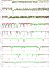 |
Fig. 1 Snapshots of the wavelength regions used in the spectral fit to the UVES spectrum of GJ 667C. The observed spectrum is represented in black, the green curves are the parts of the synthetic spectrum used in the fit. The red lines are also from the synthetic spectrum that were not used to avoid contamination by telluric features or because they did not contain relevant spectroscopic information. Unfitted deep sharp lines – especially on panels four and five from the top of the page – are non-removed telluric features. |
First comparisons of these models with observations show that the quality of computed spectra is greatly improved in comparison to older versions. The problem in previous versions of the PHOENIX models was that observed spectra in the ϵ- and γ-TiO bands could not be reproduced assuming the same effective temperature parameter (Reiners 2005). The introduction of the new equation of state apparently resolved this problem. The new models can consistently reproduce both TiO absorption bands together with large parts of the visual spectrum at very high fidelity (see Fig. 1).
As for the observed spectra, the models in our grid are also normalized to the local continuum. The regions selected for the fit were chosen as unaffected by telluric contamination and are marked in green in Fig. 1. The molecular TiO bands in the region between 705 nm to 718 nm (ϵ-TiO) and 840 nm to 848 nm (γ-TiO) are very sensitive to Teff but almost insensitive to log g. The alkali lines in the regions between 764 nm to 772 nm and 816 nm to 822 nm (K- and Na-atomic lines, respectively) are sensitive to log g and Teff. All regions are sensitive to metallicity. The simultaneous fit of all the regions to all three parameters breaks the degeneracies, leading to a unique solution of effective temperature, surface gravity and metallicity.
As the first step, a three dimensional χ2-map is produced to determine start values for the fitting algorithm. Since the model grid for the χ2-map is discrete, the real global minimum is likely to lie between grid points. We use the parameter sets of the three smallest χ2-values as starting points for the adjustment procedure. We use the IDL curvefit-function as the fitting algorithm. Since this function requires continuous parameters, we use three dimensional interpolation in the model spectra. As a fourth free parameter, we allow the resolution of the spectra to vary in order to account for possible additional broadening (astrophysical or instrumental). For this star, the relative broadening is always found to be <3% of the assumed resolution of UVES, and is statistically indistinguishable from 0. More information on the method and first results on a more representative sample of stars will be given in a forthcoming publication.
As already mentioned, the distance to the GJ 667 system comes from the Hipparcos parallax of the GJ 667AB pair and is rather uncertain (see Table 2). This, combined with the luminosity-mass calibrations in Delfosse et al. (2000), propagates into a rather uncertain mass (0.33 ± 0.02 M⊙) and luminosity estimates (0.0137 ± 0.0009 L⊙) for GJ 667C (Anglada-Escudé et al. 2012). A good trigonometric parallax measurement and the direct measurement of the size of GJ 667C using interferometry (e.g. von Braun et al. 2011) are mostly needed to refine its fundamental parameters. The updated values of the spectroscopic parameters are slightly changed from previous estimates. For example, the effective temperature used in Anglada-Escudé et al. (2012) was based on evolutionary models using the stellar mass as the input which, in turn, is derived from the rather uncertain parallax measurement of the GJ 667 system. If the spectral type were to be understood as a temperature scale, the star should be classified as an M3V-M4V instead of the M1.5V type assigned in previous works (e.g. Geballe et al. 2002). This mismatch is a well known effect on low metallicity M dwarfs (less absorption in the optical makes them appear of earlier type than solar metallicity stars with the same effective temperature). The spectroscopically derived parameters and other basic properties collected from the literature are listed in Table 2.
Stellar parameters of GJ 667C.
3. Observations and Doppler measurements
A total of 173 spectra obtained using the HARPS spectrograph (Pepe et al. 2002) have been re-analyzed using the HARPS-TERRA software (Anglada-Escudé & Butler 2012). HARPS-TERRA implements a least-squares template matching algorithm to obtain the final Doppler measurement. This method is especially well suited to deal with the highly blended spectra of low-mass stars. It only replaces the last step of a complex spectral reduction procedure as implemented by the HARPS Data Reduction Software (DRS). Such extraction is automatically done by the HARPS-ESO services and includes all the necessary steps from 2D extraction of the echelle orders, flat and dark corrections, and accurate wavelength calibration using several hundreds of Th Ar lines accross the HARPS wavelength range (Lovis & Pepe 2007). Most of the spectra (171) were extracted from the ESO archives and have been obtained by other groups over the years (e.g., Bonfils et al. 2013; Delfosse et al. 2013) covering from June 2004 to June 2010. To increase the time baseline and constrain long period trends, two additional HARPS observations were obtained between March 5th and 8th of 2012. In addition to this, three activity indices were also extracted from the HARPS spectra. These are: the S-index (proportional to the chromospheric emission of the star), the full-width-at-half-maximum of the mean line profile (or FWHM, a measure of the width of the mean stellar line) and the line bisector (or BIS, a measure of asymmetry of the mean stellar line). Both the FWHM and BIS are measured by the HARPS-DRS and were taken from the headers of the corresponding files. All these quantities might correlate with spurious Doppler offsets caused by stellar activity. In this sense, any Doppler signal with a periodicity compatible with any of these signals will be considered suspicious and will require a more detailed analysis. The choice of these indices is not arbitrary. Each of them is thought to be related to an underlying physical process that can cause spurious Doppler offsets. For example, S-index variability typically maps the presence of active regions on the stellar surface and variability of the stellar magnetic field (e.g., solar-like cycles). The line bisector and FWHM should have the same period as spurious Doppler signals induced by spots corotating with the star (contrast effects combined with stellar rotation, suppression of convection due to magnetic fields and/or Zeeman splitting in magnetic spots). Some physical processes induce spurious signals at some particular spectral regions (e.g., spots should cause stronger offsets at blue wavelengths). The Doppler signature of a planet candidate is constant over all wavelengths and, therefore, a signal that is only present at some wavelengths cannot be considered a credible candidate. This feature will be explored below to validate the reality of some of the proposed signals. A more comprehensive description of each index and their general behavior in response to stellar activity can be found elsewhere (Baliunas et al. 1995; Lovis et al. 2011). In addition to the data products derived from HARPS observations, we also include 23 Doppler measurements obtained using the PFS/Magellan spectrograph between June 2011 and October 2011 using the Iodine cell technique, and 22 HIRES/Keck Doppler measurements (both RV sets are provided in Anglada-Escudé & Butler 2012) that have lower precision but allow extending the time baseline of the observations. The HARPS-DRS also produces Doppler measurements using the so–called cross correlation method (or CCF). In the Appendices, we show that the CCF-Doppler measurements actually contain the same seven signals providing indirect confirmation and lending further confidence to the detections.
4. Statistical and physical models
The basic model of a radial velocity data set from a single telescope-instrument
combination is a sum of k Keplerian signals, with k = 0,
1, ..., a random variable describing the instrument noise, and another describing all the
excess noise in the data. The latter noise term, sometimes referred to as stellar RV jitter
(Ford 2005), includes the noise originating from
the stellar surface due to inhomogeneities, activity-related phenomena, and can also include
instrumental systematic effects. Following Tuomi
(2011), we model these noise components as Gaussian random variables with zero mean
and variances of  and
and
 , where the
former is the formal uncertainty in each measurement and the latter is the jitter that is
treated as a free parameter of the model (one for each instrument l).
, where the
former is the formal uncertainty in each measurement and the latter is the jitter that is
treated as a free parameter of the model (one for each instrument l).
Since radial velocity variations have to be calculated with respect to some reference
velocity, we use a parameter γl that describes
this reference velocity with respect to the data mean of a given instrument. For several
telescope/instrument combinations, the Keplerian signals must necessarily be the same but
the parameters γl (reference velocity) and
(jitter) cannot
be expected to have the same values. Finally, the model also includes a linear trend
 to account for very long period companions (e.g., the acceleration caused by the nearby
GJ 667AB binary). This model does not include mutual interactions between planets, which are
known to be significant in some cases (e.g. GJ 876, Laughlin
& Chambers 2001). In this case, the relatively low masses of the companions
combined with the relatively short time-span of the observations makes these effects too
small to have noticeable impact on the measured orbits. Long-term dynamical stability
information is incorporated and discussed later (see Sect. 8). Explicitly, the baseline model for the RV observations is
to account for very long period companions (e.g., the acceleration caused by the nearby
GJ 667AB binary). This model does not include mutual interactions between planets, which are
known to be significant in some cases (e.g. GJ 876, Laughlin
& Chambers 2001). In this case, the relatively low masses of the companions
combined with the relatively short time-span of the observations makes these effects too
small to have noticeable impact on the measured orbits. Long-term dynamical stability
information is incorporated and discussed later (see Sect. 8). Explicitly, the baseline model for the RV observations is ![Mathematical equation: \begin{equation} \label{eq:model} v_{l}(t_i) = \gamma_{l} + \dot{\gamma}\, (t_i-t_0) + \sum_{j=1}^{k} f(t_i, \vec{\beta}_{j}) + g_l\left[\vec{\psi}; t_{i}, z_{i}, t_{i-1}, r_{i-1}\right]\, , \end{equation}](/articles/aa/full_html/2013/08/aa21331-13/aa21331-13-eq55.png) (1)where
t0 is some reference epoch (which we arbitrarily choose as
t0 = 2 450 000 JD), g is a function
describing the specific noise properties (instrumental and stellar) of the
lth instrument on top of the estimated Gaussian uncertainties. We model
this function using first order moving average (MA) terms Tuomi et al. (2013b,a) that and on the
residual ri − 1 to the previous measurement at
ti − 1, and using linear correlation terms
with activity indices (denoted as zi). This
component of the model is typically parameterized using one or more “nuisance parameters”
ψ that are also treated as free parameters of the model. Function
f represents the Doppler model of a planet candidate with parameters
βj (Period
Pj, Doppler semi-amplitude
Kj, mean anomaly at reference epoch
M0,j, eccentricity
ej, and argument of the periastron
ωj).
(1)where
t0 is some reference epoch (which we arbitrarily choose as
t0 = 2 450 000 JD), g is a function
describing the specific noise properties (instrumental and stellar) of the
lth instrument on top of the estimated Gaussian uncertainties. We model
this function using first order moving average (MA) terms Tuomi et al. (2013b,a) that and on the
residual ri − 1 to the previous measurement at
ti − 1, and using linear correlation terms
with activity indices (denoted as zi). This
component of the model is typically parameterized using one or more “nuisance parameters”
ψ that are also treated as free parameters of the model. Function
f represents the Doppler model of a planet candidate with parameters
βj (Period
Pj, Doppler semi-amplitude
Kj, mean anomaly at reference epoch
M0,j, eccentricity
ej, and argument of the periastron
ωj).
The Gaussian white noise component of each measurement and the Gaussian jitter component
associated to each instrument enter the model in the definition of the likelihood function
L as ![Mathematical equation: \begin{equation} \label{eq:likelihood} L(m | \vec{\theta}) = \prod_{i=1}^{N} \frac{1}{\sqrt{2\pi (\sigma_{i}^{2} + \sigma_{l}^{2})}} \exp \Bigg\{ \frac{-\big[m_{i} - v_{l}(t_{i})\big]^{2}}{2(\sigma_{i}^{2} + \sigma_{l}^{2})} \Bigg\} , \end{equation}](/articles/aa/full_html/2013/08/aa21331-13/aa21331-13-eq70.png) (2)where m
stands for data and N is the number of individual
measurements. With these definitions, the posterior probability density
π(θ|m) of parameters
θ given the data m (θ includes the
orbital elements βj, the slope term
,
the instrument dependent constant offsets γl,
the instrument dependent jitter terms σl, and a
number of nuisance parameters ψ), is derived from the Bayes’ theorem as
(2)where m
stands for data and N is the number of individual
measurements. With these definitions, the posterior probability density
π(θ|m) of parameters
θ given the data m (θ includes the
orbital elements βj, the slope term
,
the instrument dependent constant offsets γl,
the instrument dependent jitter terms σl, and a
number of nuisance parameters ψ), is derived from the Bayes’ theorem as
 (3)This equation is
where the prior information enters the model through the choice of the prior density
functions π(θ). This way, the posterior density
π(θ|m) combines the new information
provided by the new data m with our prior assumptions for the parameters.
In a Bayesian sense, finding the most favored model and allowed confidence intervals
consists of the identification and exploration of the higher probability regions of the
posterior density. Unless the model of the observations is very simple (e.g., linear
models), a closed form of π(θ|m) cannot
be derived analytically and numerical methods are needed to explore its properties. The
description of the adopted numerical methods are the topic of the next subsection.
(3)This equation is
where the prior information enters the model through the choice of the prior density
functions π(θ). This way, the posterior density
π(θ|m) combines the new information
provided by the new data m with our prior assumptions for the parameters.
In a Bayesian sense, finding the most favored model and allowed confidence intervals
consists of the identification and exploration of the higher probability regions of the
posterior density. Unless the model of the observations is very simple (e.g., linear
models), a closed form of π(θ|m) cannot
be derived analytically and numerical methods are needed to explore its properties. The
description of the adopted numerical methods are the topic of the next subsection.
4.1. Posterior samplings and Bayesian detection criteria
Given a model with k Keplerian signals, we draw statistically representative samples from the posterior density of the model parameters (Eq. (3)) using the adaptive Metropolis algorithm Haario et al. (2001). This algorithm has been used successfully in e.g. Tuomi (2011), Tuomi et al. (2011) and Anglada-Escudé & Tuomi (2012). The algorithm appears to be a well suited to the fitting of Doppler data in terms of its relatively fast convergence – even when the posterior is not unimodal (Tuomi 2012) – and it provides samples that represent well the posterior densities. We use these samples to locate the regions of maximum a posteriori probability in the parameter space and to estimate each parameter confidence interval allowed by the data. We describe the parameter densities briefly by using the maximum a posteriori probability (MAP) estimates as the most probable values, i.e. our preferred solution, and by calculating the 99% Bayesian credibility sets (BCSs) surrounding these estimates. Because of the caveats of point estimates (e.g., inability to describe the shapes of posterior densities in cases of multimodality and/or non-negligible skewness), we also plot marginalized distributions of the parameters that are more important from a detection and characterization point of view, namely, velocity semi-amplitudes Kj, and eccentricities ej.
The availability of samples from the posterior densities of our statistical models also enables us to take advantage of the signal detection criteria given in Tuomi (2012). To claim that any signal is significant, we require that 1) its period is well-constrained from above and below; 2) its RV amplitude has a density that differs from zero significantly (excluded from the 99% credibility intervals); and 3) the posterior probability of the model containing k + 1 signals must be (at least) 150 times greater than that of the model containing only k signals.
The threshold of 150 on condition (3) might seem arbitrary, and although posterior probabilities also have associated uncertainties (Jenkins & Peacock 2011), we consider that such a threshold is a conservative one. As made explicit in the definition of the posterior density function π(θ|m), the likelihood function is not the only source of information. We take into account the fact that all parameter values are not equally probable prior to making the measurements via prior probability densities. Essentially, our priors are chosen as in Tuomi (2012). Of special relevance in the detection process is the prior choice for the eccentricities. Our functional choice for it (Gaussian with zero mean and σe = 0.3) is based on statistical, dynamical and population considerations and it is discussed further in the appendices (Appendix A). For more details on different prior choices, see the dedicated discussion in Tuomi & Anglada-Escudé (2013).
4.2. Log-Likelihood periodograms
Because the orbital period (or frequency) is an extremely nonlinear parameter, the orbital solution of a model with k + 1 signals typically contains many hundreds or thousands of local likelihood maxima (also called independent frequencies). In any method based on stochastic processes, there is always a chance that the global maxima of the target function is missed. Our log-likelihood periodogram (or log-L periodogram) is a tool to systematically identify periods for new candidate planets of higher probability and ensure that these areas have been well explored by the Bayesian samplings (e.g., we always attempt to start the chains close to the five most significant periodicities left in the data). A log-L periodogram consists of computing the improvement of the logarithm of the likelihood (new model with k + 1 planets) compared to the logarithm of the likelihood of the null hypothesis (only k planets) at each test period. Log-L periodograms are represented as period versus Δlog L plots, where log is always the natural logarithm. The definition of the likelihood function we use is shown in Eq. (2) and typically assumes Gaussian noise sources only (that is, different jitter parameters are included for each instrument and g = 0 in Eq. (1)).
Δlog L can also be used for estimating the frequentist
false alarm probability (FAP) of a solution using the likelihood-ratio test for
nested models. This FAP estimates what fraction of times one would recover such a
significant solution by an unfortunate arrangement of Gaussian noise. To compute this FAP
from Δlog L we used the up-to-date recipes provided by Baluev (2009). We note that that maximization of the
likelihood involves solving for many parameters simultaneously: orbital parameters of the
new candidate, all orbital parameters of the already detected signals, a secular
acceleration term ,
a zero-point γl for each instrument, and
jitter terms σl of each instrument (see Eq.
(1)). It is, therefore, a computationally
intensive task, especially when several planets are included and several thousand of test
periods for the new candidate must be explored.
As discussed in the appendices (see Sect. A.1), allowing for full Keplerian solutions at the period search level makes the method very prone to false positives. Therefore while a full Keplerian solution is typically assumed for all the previously detected k-candidates, the orbital model for the k + 1-candidate is always assumed to be circular in our standard setup. This way, our log-L periodograms represent a natural generalization of more classic hierarchical periodogram methods. This method was designed to account for parameter correlations at the detection level. If such correlations are not accounted for, the significance of new signals can be strongly biased causing both false positives and missed detections. In the study of the planet hosting M-dwarf GJ 676A (Anglada-Escudé & Tuomi 2012) and in the more recent manuscript on GJ 581 (Tuomi & Jenkins 2012), we have shown that – while log-L periodograms represent an improvement with respect to previous periodogram schemes – the aforementioned Bayesian approach has a higher sensitivity to lower amplitude signals and is less prone to false positive detections. Because of this, the use of log-L periodograms is not to quantify the significance of a new signal but to provide visual assessment of possible aliases or alternative high-likelihood solutions.
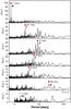 |
Fig. 2 Log-likelihood periodograms for the seven candidate signals sorted by significance. While the first six signals are easily spotted, the seventh is only detected with log-L periodograms if all orbits are assumed to be circular. |
Log-L periodograms implicitly assume flat priors for all the free parameters. As a result, this method provides a quick way of assessing the sensitivity of a detection against a choice of prior functions that are different from uniform. As discussed later, the sixth candidate is only confidently spotted using log-L periodograms (our detection criteria is FAP < 1%) when the orbits of all the candidates are assumed to be circular. This is the red line beyond which our detection criteria becomes strongly dependent on our choice of prior on the eccentricity. The same applies to the seventh tentative candidate signal.
5. Signal detection and confidences
As opposed to other systems analyzed with the same techniques (e.g. Tau Ceti or HD 40307, Tuomi et al. 2013a,b), we found that for GJ 667C the simplest model (g = 0 in Eq. (1)) already provides a sufficient description of the data. For brevity, we omit here all the tests done with more sophisticated parameterizations of the noise (see Appendix C) that essentially lead to unconstrained models for the correlated noise terms and the same final results. In parallel with the Bayesian detection sequence, we also illustrate the search using log-L periodograms. In all that follows we use the three datasets available at this time: HARPS-TERRA, HIRES and PFS. We use the HARPS-TERRA Doppler measurements instead of CCF ones because TERRA velocities have been proven to be more precise on stable M-dwarfs (Anglada-Escudé & Butler 2012).
Relative posterior probabilities and log-Bayes factors of models ℳk with k Keplerian signals given the combined HARPS-TERRA, HIRES, and PFS RV data of GJ 667C.
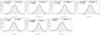 |
Fig. 3 Marginalized posterior densities for the Doppler semi-amplitudes of the seven reported signals. |
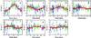 |
Fig. 4 RV measurements phase-folded to the best period for each planet. Brown circles are HARPS-TERRA velocities, PFS velocities are depicted as blue triangles, and HIRES velocities are green triangles. Red squares are averages on 20 phase bins of the HARPS-TERRA velocities. The black line corresponds to the best circular orbital fit (visualization purposes only). |
The first three periodicities (7.2 days, 28.1 days and 91 days) were trivially spotted using Bayesian posterior samplings and the corresponding log-L periodograms. These three signals were already reported by Anglada-Escudé et al. (2012) and Delfosse et al. (2013), although the last one (signal d, at 91 days) remained uncertain due to the proximity of a characteristic time-scale of the star’s activity. This signal is discussed in the context of stellar activity in Sect. 6. Signal d has a MAP period of 91 days and would correspond to a candidate planet with a minimum mass of ~5 M⊕.
After that, the log-L periodogram search for a fourth signal indicates a double-peaked likelihood maximum at 53 and 62 days – both candidate periods receiving extremely low false-alarm probability estimates (see Fig. 2). Using the recipes in Dawson & Fabrycky (2010), it is easy to show that the two peaks are the yearly aliases of each other. Accordingly, our Bayesian samplings converged to either period equally well giving slightly higher probability to the 53-day orbit (×6). In both cases, we found that including a fourth signal improved the model probability by a factor >103. In appendix B.2 we provide a detailed analysis and derived orbital properties of both solutions and show that the precise choice of this fourth period does not substantially affect the confidence of the rest of the signals. As will be shown at the end of the detection sequence, the most likely solution for this candidate corresponds to a minimum mass of 2.7 M⊕ and a period of 62 days.
After including the fourth signal, a fifth signal at 39.0 days shows up conspicuously in the log-L periodograms. In this case, the posterior samplings always converged to the same period of 39.0 days without difficulty (signal f). Such a planet would have a minimum mass of ~2.7 M⊕. Given that the model probability improved by a factor of 5.3 × 10⁵ and that the FAP derived from the log-L periodogram is 0.45%, the presence of this periodicity is also supported by the data without requiring further assumptions.
The Bayesian sampling search for a sixth signal always converged to a period of 260 days that also satisfied our detection criteria and increased the probability of the model by a factor of 4 × 10³. The log-L periodograms did spot the same signal as the most significant one but assigned a FAP of ~20% to it. This apparent contradiction is due to the prior on the eccentricity. That is, the maximum likelihood solution favors a very eccentric orbit for the Keplerian orbit at 62 days (ee ~ 0.9), which is unphysical and absorbs variability at long timescales through aliases. To investigate this, we performed a log-L periodogram search assuming circular orbits for all the candidates. In this case, the 260-day period received a FAP of 0.5% which would then qualify as a significant detection. Given that the Bayesian detection criteria are well satisfied and that the log-L periodograms also provide substantial support for the signal, we also include it in the model (signal g). Its amplitude would correspond to a planet with a minimum mass of 4.6 M⊕.
When performing a search for a seventh signal, the posterior samplings converged consistently to a global probability maximum at 17 days (Msini ~ 1.1 M⊕) which improves the model probability by a factor of 230. The global probability maximum containing seven signals corresponds to a solution with a period of 62 days for planet e. This solution has a total probability ~16 times larger than the one with Pe = 53 days. Although such a difference is not large enough to make a final decision on which period is preferred, from now on we will assume that our reference solution is the one with Pe = 62.2 days. The log-L periodogram also spotted the same seventh period as the next favored one but only when all seven candidates were assumed to have circular orbits. Given that this seventh signal is very close to the Bayesian detection limit, and based on our experience on the analysis of similar datasets (e.g., GJ 581, Tuomi & Jenkins 2012), we concede that this candidate requires more measurements to be securely confirmed. With a minimum mass of only ~1.1 M⊕, it would be among the least massive exoplanets discovered to date.
As a final comment we note that, as in Anglada-Escudé et al. (2012) and Delfosse et al. (2013), a linear trend was always included in the model. The most likely origin of such a trend is gravitational acceleration caused by the central GJ 667AB binary. Assuming a minimum separation of 230 AU, the acceleration in the line-of-sight of the observer can be as large as 3.7 m s-1, which is of the same order of magnitude as the observed trend of ~2.2 m s-1 yr-1. We remark that the trend (or part of it) could also be caused by the presence of a very long period planet or brown dwarf. Further Doppler follow-up, astrometric measurements, or direct imaging attempts of faint companions might help addressing this question.
In summary, the first five signals are easily spotted using Bayesian criteria and log-L periodograms. The global solution containing seven-Keplerian signals prefers a period of 62.2 days for signal e, which we adopt as our reference solution. Still, a period of 53 days for the same signal cannot be ruled out at the moment. The statistical significance of a 6th periodicity depends on the prior choice for the eccentricity, but the Bayesian odds ratio is high enough to propose it as a genuine Keplerian signal. The statistical significance of the seventh candidate (h) is close to our detection limit and more observations are needed to fully confirm it.
6. Activity
Reference orbital parameters and their corresponding 99% credibility intervals.
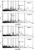 |
Fig. 5 Top two panels. Log-L periodograms for up to 2 signals in the S-index. The most likely periods of the proposed planet candidates are marked as vertical lines. Bottom two panels. Log-L periodograms for up to 2 signals in the FWHM. Given the proximity of these two signals, it is possible that both of them originate from the same feature (active region corotating with the star) that is slowly evolving with time. |
In addition to random noise (white or correlated), stellar activity can also generate spurious Doppler periodicities that can mimic planetary signals (e.g., Lovis et al. 2011; Reiners et al. 2013). In this section we investigate whether there are periodic variations in the three activity indices of GJ 667C (S-index, BIS and FWHM are described in Sect. 3). Our general strategy is the following: if a significant periodicity is detected in any of the indices and such periodicity can be related to any of the candidate signals (same period or aliases), we add a linear correlation term to the model and compute log-L periodograms and new samplings of the parameter space. If the data were better described by the correlation term rather than a genuine Doppler signal, the overall model probability would increase and the planet signal in question should decrease its significance (even disappear).
Log-L periodogram analysis of two activity indices (S-index but specially the FWHM) show a strong periodic variability at 105 days. As discussed in Anglada-Escudé et al. (2012) and Delfosse et al. (2013), this cast some doubt on the candidate at 91 days (d). Despite the fact that the 91-day and 105-day periods are not connected by first order aliases, the phase sampling is sparse in this period domain (see phase–folded diagrams of the RV data for the planet d candidate in Fig. 4) and the log-L periodogram for this candidate also shows substantial power at 105 days. From the log-L periodograms in Fig. 2, one can directly obtain the probability ratio of a putative solution at 91 days versus one with a period of 105 days when no correlation terms are included. This ratio is 6.8 × 10⁴, meaning that the Doppler period at 91 days is largely favored over the 105-day one. All Bayesian samplings starting close to the 105-day peak ended-up converging on the signal at 91 day. We then applied our validation procedure by inserting linear correlation terms in the model (g = CF × FWHMi or g = CS × Si), in Eq. (1)) and computed both log-L periodograms and Bayesian samplings with CF and CS as free parameters. In all cases the Δlog L between 91 and 105 days slightly increased, thus supporting the conclusion that the signal at 91 days is of planetary origin. For example, the ratio of likelihoods between the 91 and 105 day signals increased from 6.8 × 10⁴ to 3.7 × 10⁶ when the correlation term with the FWHM was included (see Fig. 6). The Bayesian samplings including the correlation term did not improve the model probability (see Appendix C) and still preferred the 91-day signal without any doubt. We conclude that this signal is not directly related to the stellar activity and therefore is a valid planet candidate.
Given that activity might induce higher order harmonics in the time-series, all seven candidates have been analyzed and double-checked using the same approach. Some more details on the results from the samplings are given in the Appendix C.2. All candidates -including the tentative planet candidate h- passed all these validation tests without difficulties.
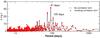 |
Fig. 6 Log-likelihood periodograms for planet d (91 days) including the correlation term (red dots) compared to the original periodogram without this term (black line). The inclusion of the correlation term increases the contrast between the peaks at 91 and 105 days, favoring the interpretation of the 91 days signals as a genuine planet candidate. |
7. Tests for quasi-periodic signals
Most significant periods as extracted using log -L periodograms on subsamples of the first Nobs measurements.
Activity induced signals and superposition of several independent signals can be a source of confusion and result in detections of “apparent” false positives. In an attempt to quantify how much data is necessary to support our preferred global solution (with seven planets) we applied the log-L periodogram analysis method to find the solution as a function of the number of data points. For each dataset, we stopped searching when no peak above FAP 1% was found. The process was fully automated so no human-biased intervention could alter the detection sequence. The resulting detection sequences are show in Table 5. In addition to observing how the complete seven-planet solution slowly emerges from the data one can notice that for Nobs < 100 the k = 2 and k = 3 solutions converge to a strong signal at ~100 days. This period is dangerously close to the activity one detected in the FWHM and S-index time-series. To explore what could be the cause of this feature (perhaps the signature of a quasi-periodic signal), we examined the Nobs = 75 case in more detail and made a supervised/visual analysis of that subset.
The first 7.2 days candidate could be easily extracted. We then computed a periodogram of the residuals to figure out if there were additional signals left in the data. In agreement with the automatic search, the periodogram of the residuals (bottom of Fig. 7) show a very strong peak at ~100 days. The peak was so strong that we went ahead and assessed its significance. It had a very low FAP (<0.01%) and also satisfied our Bayesian detectability criteria. We could have searched for additional companions, but let us assume we stopped our analysis here. In this case, we would have concluded that two signals were strongly present (7.2 days and 100 days). Because of the proximity with a periodicity in the FWHM-index ( 105 days), we would have expressed our doubts about the reality of the second signal so only one planet candidate would have been proposed (GJ 667Cb).
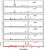 |
Fig. 7 Sequence of periodograms obtained from synthetic noiseless data generated on the first 75 epochs. The signals in Table 4 were sequentially injected from top to bottom. The bottom panel is the periodogram to the real dataset after removing the first 7.2 days planet candidate. |
With 228 RV measurements in hand (173 HARPS-TERRA, 23 PFS and 22 from HIRES) we know that such a conclusion is no longer compatible with the data. For example, the second and third planets are very consistently detected at 28 and 91 days. We investigated the nature of that 100 day signal using synthetic subsets of observations as follows. We took our preferred seven-planet solution and generated the exact signal we would expect if we only had planet c (28 days) in the first 75 HARPS-TERRA measurements (without noise). The periodogram of such a noiseless time-series (top panel in Fig. 7) was very different from the real one. Then, we sequentially added the rest of the signals. As more planets were added, the periodogram looked closer to the one from the real data. This illustrates that we would have reached the same wrong conclusion even with data that had negligible noise. How well the general structure of the periodogram was recovered after adding all of the signals is rather remarkable (comparing the bottom two panels in Fig. 7). While this is not a statistical proof of significance, it shows that the periodogram of the residuals from the 1-planet fit (even with only 75 RVs measurements) is indeed consistent with the proposed seven-planet solution without invoking the presence of quasi-periodic signals. This experiment also shows that, until all stronger signals could be well-decoupled (more detailed investigation showed this happened at about Nobs ~ 140), proper and robust identification of the correct periods was very difficult. We repeated the same exercise with Nobs = 100, 120 and 173 (all HARPS measurements) and obtained identical behavior without exception (see panels in Fig. 8). Such an effect is not new and the literature contains several examples that cannot be easily explained by simplistic aliasing arguments- e.g., see GJ 581d (Udry et al. 2007; Mayor et al. 2009) and HD 125612b/c (Anglada-Escudé et al. 2010; Lo Curto et al. 2010). The fact that all signals detected in the velocity data of GJ 667C have similar amplitudes – except perhaps candidate b which has a considerably higher amplitude – made this problem especially severe. In this sense, the currently available set of observations are a subsample of the many more that might be obtained in the future, so it might happen that one of the signals we report “bifurcates” into other periodicities. This experiment also suggests that spectral information beyond the most trivial aliases can be used to verify and assess the significance of future detections (under investigation).
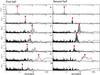 |
Fig. 9 Periodograms on first and second half of the time series as obtained when all signals except one were removed from the data. Except for signal h, all signals are significantly present in both halves and could have been recovered using either half if they had been in single planet systems. |
7.1. Presence of individual signals in one half of the data
As an additional verification against quasi-periodicity, we investigated if the signals were present in the data when it was divided into two halves. The first half corresponds to the first 86 HARPS observations and the second half covers the remaining data. The data from PFS and HIRES were not used for this test. The experiment consists of removing all signals except for one, and then computing the periodogram on those residuals (first and second halfs separately). If a signal is strongly present in both halfs, it should, at least, emerge as substantially significant. All signals except for the seventh one passed this test nicely. That is, in all cases except for h, the periodograms prominently display the non-removed signal unambiguously. Besides demonstrating that all signals are strongly present in the two halves, it also illustrates that any of the candidates would have been trivially spotted using periodograms if it had been orbiting alone around the star. The fact that each signal was not spotted before (Anglada-Escudé et al. 2012; Delfosse et al. 2013) is a consequence of an inadequate treatment of signal correlations when dealing with periodograms of the residuals only. Both the described Bayesian method and the log-likelihood periodogram technique are able to deal with such correlations by identifying the combined global solution at the period search level. As for other multiplanet systems detected using similar techniques (Tuomi et al. 2013b; Anglada-Escudé & Tuomi 2012), optimal exploration of the global probability maxima at the signal search level is essential to properly detect and assess the significance of low mass multiplanet solutions, especially when several signals have similar amplitudes close to the noise level of the measurements.
Summarizing these investigations and validation of the signals against activity, we conclude that
-
Up to seven periodic signals are detected in the Dopplermeasurements of GJ 667C data, with the last (seventh) signal veryclose to our detection threshold.
-
The significance of the signals are not affected by correlations with activity indices and we could not identify any strong wavelength dependence with any of them.
-
The first six signals are strongly present in subsamples of the data. Only the seventh signal is unconfirmed using half of the data alone. Our analysis indicates that any of the six stronger signals would had been robustly spotted with half the available data if each had been orbiting alone around the host star.
-
Signal correlations in unevenly sampled data are the reason why Anglada-Escudé et al. (2012) and Delfosse et al. (2013) only reported three of them. This is a known problem when assessing the significance of signals using periodograms of residuals only (see Anglada-Escudé & Tuomi 2012, as another example).
Given the results of these validation tests, we promote six of the signals (b, c, d, e, f, g) to planet candidates. For economy of language, we will refer to them as planets but the reader must remember that, unless complementary and independent verification of a Doppler signal is obtained (e.g., transits), they should be called planet candidates. Verifying the proposed planetary system against dynamical stability is the purpose of the next section.
8. Dynamical analysis
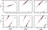 |
Fig. 10 Result of the stability analysis of 80 000 six-planet solutions in the plane of initial semi-major axis a vs. initial mean longitude λ obtained from a numerical integration over T ≈ 7000 years. Each initial condition is represented as a point. Initial conditions leading to an immediate disintegration of the system are shown as gray dots. Initial conditions that lead to stable motion for at least 1 Myr are shown as red points (D < 10-5). Black crosses represent the most stable solutions (D < 10-6), and can last over many Myr. |
One of the by-products of the Bayesian analysis described in the previous sections, are numerical samples of statistically allowed parameter combinations. The most likely orbital elements and corresponding confidence levels can be deduced from these samples. In Table 4 we give the orbital configuration for a planetary system with seven planets around GJ 667C, which is preferred from a statistical point of view. To be sure that the proposed planetary system is physically realistic, it is necessary to confirm that these parameters not only correspond to the solution favored by the data, but also constitute a dynamically stable configuration. Due to the compactness of the orbits, abundant resonances and therefore complex interplanetary interactions are expected within the credibility intervals. To slightly reduce this complexity and since evidence for planet h is weak, we split our analysis and present – in the first part of this section – the results for the six-planet solution with planets b to g. The dynamical feasibility of the seven-planet solution is then assessed by investigating the semi-major axis that would allow introducing a seventh planet with the characteristics of planet h.
Astrocentric orbital elements of solution S6.
8.1. Finding stable solutions for six planets
A first thing to do is to extract from the Bayesian samplings those orbital configurations that allow stable planetary motion over long time scales, if any. Therefore we tested the stability of each configuration by a separate numerical integration using the symplectic integrator SABA2 of Laskar & Robutel (2001) with a step size τ = 0.0625 days. In the integration, we included a correction term to account for general relativistic precession. Tidal effects were neglected for these runs. Possible effects of tides are discussed separately in Sect. 9.4. The integration was stopped if any of the planets went beyond 5 AU or planets approached each other closer than 10-4 AU.
The stability of those configurations that survived the integration time span of 104 orbital periods of planet g (i.e. ≈7000 years), was then determined using frequency analysis (Laskar 1993). For this we computed the stability index Dk for each planet k as the relative change in its mean motion nk over two consecutive time intervals as was done in Tuomi et al. (2013b). For stable orbits the computed mean motion in both intervals will be almost the same and therefore Dk will be very small. We note that this also holds true for planets captured inside a mean-motion resonance (MMR), as long as this resonance helps to stabilize the system. As an index for the total stability of a configuration we used D = max(| Dk |). The results are summarized in Fig. 10. To generate Fig. 10, we extracted a subsample of 80 000 initial conditions from the Bayesian samplings. Those configurations that did not reach the final integration time are represented as gray dots. By direct numerical integration of the remaining initial conditions, we found that almost all configurations with D < 10-5 survive a time span of 1 Myr. This corresponds to ~0.3 percent of the total sample. The most stable orbits we found (D < 10-6) are depicted as black crosses.
In Fig. 10 one can see that the initial conditions taken from the integrated 80 000 solutions are already confined to a very narrow range in the parameter space of all possible orbits. This means that the allowed combinations of initial a and λ are already quite restricted by the statistics. By examining Fig. 10 one can also notice that those initial conditions that turned out to be long-term stable are quite spread out along the areas where the density of Bayesian states is higher. Also, for some of the candidates (d, f and g), there are regions were no orbit was found with D < 10-5. The paucity of stable orbits at certain regions indicate areas of strong chaos within the statistically allowed ranges (likely disruptive mean-motion resonances) and illustrate that the dynamics of the system are far from trivial.
The distributions of eccentricities are also strongly affected by the condition of dynamical stability. In Fig. 11 we show the marginalized distributions of eccentricities for the sample of all the integrated orbits (gray histograms) and the distribution restricted to relatively stable orbits (with D < 10-5, red histograms). We see that, as expected, stable motion is only possible with eccentricities smaller than the mean values allowed by the statistical samples. The only exceptions are planets b and g. These two planet candidates are well separated from the other candidates. As a consequence, their probability densities are rather unaffected by the condition of long-term stability. We note here that the information about the dynamical stability has been used only a posteriori. If we had used long-term dynamics as a prior (e.g., assign 0 probability to orbits with D > 10-5), moderately eccentric orbits would have been much more strongly suppressed than with our choice of prior function (Gaussian distribution of zero mean and σ = 0.3, see Appendix A.1). In this sense, our prior density choice provides a much softer and uninformative constraint than the dynamical viability of the system.
In the following we will use the set of initial conditions that gave the smallest D for a detailed analysis and will refer to it as S6. In Table 6, we present the masses and orbital parameters of S6, and propose it as the favored configuration. To double check our dynamical stability results, we also integrated S6 for 108 years using the HNBody package (Rauch & Hamilton 2002) including general relativistic corrections and a time step of τ = 10-3 years1.
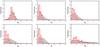 |
Fig. 11 Marginalized posterior densities for the orbital eccentricities of the six planet solution (b, c, d, in the first row; e, f, g in the second) before (gray histogram) and after (red histogram) ruling out dynamically unstable configurations. |
8.2. Secular evolution
Although the dynamical analysis of such a complex system with different, interacting resonances could be treated in a separate paper, we present here a basic analysis of the dynamical architecture of the system. From studies of the solar system, we know that, in the absence of mean motion resonances, the variations in the orbital elements of the planets are governed by the so-called secular equations. These equations are obtained after averaging over the mean longitudes of the planets. Since the involved eccentricities for GJ 667C are small, the secular system can be limited here to its linear version, which is usually called a Laplace-Lagrange solution (for details see Laskar 1990). Basically, the solution is obtained from a transformation of the complex variables zk = ekeıϖk into the proper modes uk. Here, ek are the eccentricities and ϖk the longitudes of the periastron of planet k = b,c,...,g. The proper modes uk determine the secular variation of the eccentricities and are given by uk ≈ ei(gkt + φk).
Since the transformation into the proper modes depends only on the masses and semi-major axes of the planets, the secular frequencies will not change much for the different stable configurations found in Fig. 10. Here we use solution S6 to obtain numerically the parameters of the linear transformation by a frequency analysis of the numerically integrated orbit. The secular frequencies gk and the phases φk are given in Table 7. How well the secular solution describes the long-term evolution of the eccentricities can be readily seen in Fig. 12.
Fundamental secular frequencies gk, phases φk and corresponding periods of the six-planet solution.
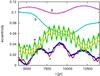 |
Fig. 12 Evolution of the eccentricities of solution S6. Colored lines give the eccentricity as obtained from a numerical integration. The thin black lines show the eccentricity of the respective planet as given by the linear, secular approximation. Close to each line we give the name of the corresponding planet. |
From Fig. 12, it is easy to see that there exists a strong secular coupling between all the inner planets. From the Laplace-Lagrange solution, we find that the long-term variation of the eccentricities of these planets is determined by the secular frequency g1 − g4 with a period of ≈17 000 years. Here, the variation in eccentricity of planet b is in anti-phase to that of planets c to f due to the exchange of orbital angular momentum. On shorter time scales, we easily spot in Fig. 12 the coupling between planets d and e with a period of ≈600 years (g1 − g5), while the eccentricities of planets c and f vary with a period of almost 3000 years (g1 + g4). Such couplings are already known to prevent close approaches between the planets (Ferraz-Mello et al. 2006). As a result, the periastron of the planets are locked and the difference Δϖ between any of their ϖ librates around zero.
Although the eccentricities show strong variations, these changes are very regular and their maximum values remain bounded. From the facts that 1) the secular solution agrees so well with numerically integrated orbits; and 2) at the same time the semi-major axes remain nearly constant (Table 8), we can conclude that S6 is not affected by strong MMRs.
Nevertheless, MMRs that can destabilize the whole system are within the credibility intervals allowed by the samplings and not far away from the most stable orbits. Integrating some of the initial conditions marked as chaotic in Fig. 10 one finds that, for example, planets d and g are in some of these cases temporarily trapped inside a 3:1 MMR, causing subsequent disintegration of the system.
Minimum and maximum values of the semi-major axes and eccentricities during a run of S6 over 10 Myr.
8.3. Including planet h
After finding a non-negligible set of stable six-planet solutions, it is tempting to look for more planets in the system. From the data analysis, one even knows the preferred location of such a planet. We first considered doing an analysis similar to the one for the six-planet case using the Bayesian samples for the seven-planet solution. As shown in previous sections, the subset of stable solutions found by this approach is already small compared to the statistical samples in the six-planet case (~0.3%). Adding one more planet (five extra dimensions) can only shrink the relative volume of stable solutions further. Given the large uncertainties on the orbital elements of h, we considered this approach too computationally expensive and inefficient.
As a first approximation to the problem, we checked whether the distances between neighboring planets are still large enough to allow stable motion. In Chambers et al. (1996) the mean lifetime for coplanar systems with small eccentricities is estimated as a function of the mutual distance between the planets, their masses and the number of planets in the system. From their results, we can estimate the expected lifetime for the seven-planet solution to be at least 108 years.
Motivated by this result, we explored the phase space around the proposed orbit for the seventh planet. To do this, we use solution S6 and placed a fictitious planet with 1.1 M⊕ (the estimated mass of planet h as given in Table 4) in the semi-major axis range between 0.035 and 0.2 AU (step size of 0.001 AU) varying the eccentricity between 0 and 0.2 (step size of 0.01). The orbital angles ω and M0 were set to the values of the statistically preferred solution for h (see Table 4). For each of these initial configurations, we integrated the system for 104 orbits of planet g and analyzed stability of the orbits using the same secular frequency analysis. As a result, we obtained a value of the chaos index D at each grid point. Figure 13 shows that the putative orbit of h appears right in the middle of the only island of stability left in the inner region of the system. By direct numerical integration of solution S6 together with planet h at its nominal position, we found that such a solution is also stable on Myr timescales. With this we conclude that the seventh signal detected by the Bayesian analysis also belongs to a physically viable planet that might be confirmed with a few more observations.
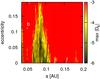 |
Fig. 13 Stability plot of the possible location of a 7th planet in the stable S6 solution (Table 5). We investigate the stability of an additional planet with 1.1 Earth masses around the location found by the Bayesian analysis. For these integrations, we varied the semi-major axis and eccentricity of the putative planet on a regular grid. The orbital angles ω and M0 were set to the values of the statistically preferred solution, while the inclination was fixed to zero. The nominal positions of the planets as given in Table 6 are marked with white crosses. |
8.4. An upper limit for the masses
Due to the lack of reported transit, only the minimum masses are known for the planet candidates. The true masses depend on the unknown inclination i of the system to the line-of-sight. In all the analysis presented above, we implicitly assume that the GJ 667C system is observed edge-on (i = 90°) and that all true masses are equal to the minimum mass Msini. As shown in the discussion on the dynamics, the stability of the system is fragile in the sense that dynamically unstable configurations can be found close in the parameter space to the stable ones. Therefore, it is likely that a more complete analysis could set strong limitations on the maximum masses allowed to each companion. An exploration of the total phase space including mutual inclinations would require too much computational resources and is beyond the scope of this paper. To obtain a basic understanding of the situation, we only search for a constraint on the maximum masses of the S6 solution assuming co-planarity. Decreasing the inclination of the orbital plane in steps of 10°, we applied the frequency analysis to the resulting system. By making the planets more massive, the interactions between them become stronger, with a corresponding shrinking of the areas of stability. In this experiment, we found that the system remained stable for at least one Myr for an inclination down to i = 30°. If this result can be validated by a much more extensive exploration of the dynamics and longer integration times (in prep.), it would confirm that the masses of all the candidates are within a factor of 2 of the minimum masses derived from Doppler data. Accordingly, c, f and e would be the first dynamically confirmed super-Earths (true masses below 10 M⊕) in the habitable zone of a nearby star.
9. Habitability
Planets h–d receive 20–200% of the Earth’s current insolation, and hence should be evaluated in terms of potential habitability. Traditionally, analyses of planetary habitability begin with determining if a planet is in the habitable zone (Dole 1964; Hart 1979; Kasting et al. 1993; Selsis et al. 2007; Kopparapu et al. 2013), but many factors are relevant. Unfortunately, many aspects cannot presently be determined due to the limited characterization derivable from RV observations. However, we can explore the issues quantitatively and identify those situations in which habitability is precluded, and hence determine which of these planets could support life. In this section we provide a preliminary analysis of each potentially habitable planet in the context of previous results, bearing in mind that theoretical predictions of the most relevant processes cannot be constrained by existing data.
9.1. The habitable zone
The HZ is defined at the inner edge by the onset of a “moist greenhouse”, and at the outer edge by the “maximum greenhouse” (Kasting et al. 1993). Both of these definitions assume that liquid surface water is maintained under an Earth-like atmosphere. At the inner edge, the temperature near the surface becomes large enough that water cannot be confined to the surface and water vapor saturates the stratosphere. From there, stellar radiation can dissociate the water and hydrogen can escape. Moreover, as water vapor is a greenhouse gas, large quantities in the atmosphere can heat the surface to temperatures that forbid the liquid phase, rendering the planet uninhabitable. At the outer edge, the danger is global ice coverage. While greenhouse gases like CO2 can warm the surface and mitigate the risk of global glaciation, CO2 also scatters starlight via Rayleigh scattering. There is therefore a limit to the amount of CO2 that can warm a planet as more CO2 actually cools the planet by increasing its albedo, assuming a moist or runaway greenhouse was never triggered.
We use the most recent calculations of the HZ (Kopparapu et al. 2013) and find, for a 1 Earth-mass planet, that the inner and outer boundaries of the habitable zone for GJ 667C lie between 0.095–0.126 AU and 0.241–0.251 AU respectively. We will adopt the average of these limits as a working definition of the HZ: 0.111 – 0.246 AU. At the inner edge, larger mass planets resist the moist greenhouse and the HZ edge is closer in, but the outer edge is almost independent of mass. Kopparapu et al. (2013) find that a 10 M⊕ planet can be habitable 5% closer to the star than a 1 M⊕ planet. However, we must bear in mind that the HZ calculations are based on 1-dimensional photochemical models that may not apply to slowly rotating planets, a situation likely for planets c, d, e, f and h (see below).
From these definitions, we find that planet candidate h (a = 0.0893 AU) is too hot to be habitable, but we note its semi-major axis is consistent with the most optimistic version of the HZ. Planet c (a = 0.125 AU) is close to the inner edge but is likely to be in the HZ, especially since it has a large mass. Planets f and e are firmly in the HZ. Planet d is likely beyond the outer edge of the HZ, but the uncertainty in its orbit prevents a definitive assessment. Thus, we conclude that planets c, f, and e are in the HZ, and planet d might be, i.e.there up to four potentially habitable planets orbiting GJ 667C.
Recently, Abe et al. (2011) pointed out that planets with small, but non-negligible, amounts of water have a larger HZ than Earth-like planets. From their definition, both h and d are firmly in the HZ. However, as we discuss below, these planets are likely water-rich, and hence we do not use the Abe et al. (2011) HZ here.
9.2. Composition
Planet formation is a messy process characterized by scattering, migration, and giant impacts. Hence precise calculations of planetary composition are presently impossible, but see Bond et al. (2010), Carter-Bond et al. (2012) for some general trends. For habitability, our first concern is discerning if a planet is rocky (and potentially habitable) or gaseous (and uninhabitable). Unfortunately, we cannot even make this rudimentary evaluation based on available data and theory. Without radii measurements, we cannot determine bulk density, which could discriminate between the two. The least massive planet known to be gaseous is GJ 1214 b at 6.55 M⊕ (Charbonneau et al. 2009), and the largest planet known to be rocky is Kepler-10 b at 4.5 M⊕ (Batalha et al. 2011). Modeling of gas accretion has found that planets smaller than 1 M⊕ can accrete hydrogen in certain circumstances (Ikoma et al. 2001), but the critical mass is likely larger (Lissauer et al. 2009). The planets in this system lie near these masses, and hence we cannot definitively say if any of these planets are gaseous.
Models of rocky planet formation around M dwarfs have found that those that accrete from primordial material are likely to be sub-Earth mass (Raymond et al. 2007) and volatile-poor (Lissauer 2007). In contrast, the planets orbiting GJ 667C are super-Earths in a very packed configuration summing up to >25 M⊕ inside 0.5 AU. Therefore, the planets either formed at larger orbital distances and migrated in (e.g. Lin et al. 1996), or additional dust and ice flowed inward during the protoplanetary disk phase and accumulated into the planets Hansen & Murray (2012, 2013). The large masses disfavor the first scenario, and we therefore assume that the planets formed from material that condensed beyond the snow-line and are volatile rich. If not gaseous, these planets contain substantial water content, which is a primary requirement for life (and negates the dry-world HZ discussed above). In conclusion, these planets could be terrestrial-like with significant water content and hence are potentially habitable.
9.3. Stellar activity and habitability
Stellar activity can be detrimental to life as the planets can be bathed in high energy photons and protons that could strip the atmosphere or destroy ozone layers. In quiescence, M dwarfs emit very little UV light, so the latter is only dangerous if flares occur frequently enough that ozone does not have time to be replenished (Segura et al. 2010). As already discussed in Sect. 2, GJ 667C appears to be relatively inactive (indeed, we would not have been able to detect planetary signals otherwise), and so the threat to life is small today. If the star was very active in its youth – with mega-flares like those on the equal mass star AD Leo (Hawley & Pettersen 1991) – any life on the surface of planets might have been difficult during those days (Segura et al. 2010). While M dwarfs are likely to be active for much longer time than the Sun (West et al. 2008; Reiners & Mohanty 2012), GJ 667C is not active today and there is no reason to assume that life could not form after an early phase of strong stellar activity.
9.4. Tidal effects
Timescales for the planets’ tidal despinning in units of Myr.
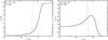 |
Fig. 14 Tidal evolution of the spin properties of planet GJ 667C f. Solid lines depict predictions from constant-time-lag theory (“CTL”), while dashed lines illustrate those from a constant-phase-lag model (“CPL”). All tracks assume a scenario similar to the “base” configuration (see text and Table 9). Left: despinning for an assumed initial rotation period of one day. The CPL model yields tidal locking in less than 5 Myr, and CTL theory predicts about 20 Myr for tidal locking. Right: tilt erosion of an assumed initial Earth-like obliquity of 23.5°. Time scales for both CPL and CTL models are similar to the locking time scales. |
Planets in the HZ of low-mass stars may be subject to strong tidal distortion, which can lead to long-term changes in orbital and spin properties (Dole 1964; Kasting et al. 1993; Barnes et al. 2008; Heller et al. 2011), and tidal heating (Jackson et al. 2008; Barnes et al. 2009, 2013). Both of these processes can affect habitability, so we now consider tidal effects on planets c, d, e, f and h.
Tides will first spin-lock the planetary spin and drive the obliquity to either 0 or π. The timescale for these processes is a complex function of orbits, masses, radii and spins, (see e.g. Darwin 1880; Hut 1981; Ferraz-Mello et al. 2008; Leconte et al. 2010) but for super-Earths in the HZ of a ~0.3 M⊙ star, Heller et al. (2011) found that tidal locking should occur in 106–109 years. We have used both the constant-time-lag and constant-phase-lag tidal models described in Heller et al. (2011) and Barnes et al. (2013; Ferraz-Mello et al. see also 2008; Leconte et al. see also 2010), to calculate how long tidal locking could take for these planets. We consider two possibilities. Our baseline case is very similar to that of Heller et al. (2011) in which the planets initially have Earth-like properties: a 1-day rotation period, an obliquity of 23.5° and the current tidal dissipation of the Earth (a tidal Q of 12-Yoder 1995 or time lag of 638 s-Lambeck 1977; Neron de Surgy & Laskar 1997). We also consider an extreme, but plausible, case that maximizes the timescale for tidal locking: 8-h rotation period, obliquity of 89.9° and a tidal Q of 1000 or time lag of 6.5 s. In Table 9 we show the time for the obliquity to erode to 1°, tero, and the time to reach the pseudo-synchronous rotation period, tlock.
In Fig. 14, we depict the tidal evolution of the rotation period (left panel) and obliquity (right panel) for planet f as an example. The assumed initial configuration is similar to the “base” scenario. Time scales for rotational locking and tilt erosion are similar to those shown in Table 92.
As these planets are on nearly circular orbits, we expect tidally-locked planets to be synchronously rotating, although perhaps when the eccentricity is relatively large pseudo-synchronous rotation could occur (Goldreich 1966; Murray & Dermott 1999; Barnes et al. 2008; Correia et al. 2008; Ferraz-Mello et al. 2008; Makarov & Efroimsky 2013). From Table 9 we see that all the planets h–f are very likely synchronous rotators, planet e is likely to be, but planet d is uncertain. Should these planets have tenuous atmospheres (<0.3 bar), then they may not support a habitable surface (Joshi et al. 1997). Considerable work has shown that thicker atmospheres are able to redistribute dayside heat to produce clement conditions (Joshi et al. 1997; Joshi 2003; Edson et al. 2011; Pierrehumbert 2011; Wordsworth et al. 2011). As we have no atmospheric data, we assert that tidal locking does not preclude habitability for any of the HZ planets.
During the tidal despinning, tidal heat can be generated as dissipation transforms rotational energy into frictional heat. In some cases, the heating rates can be large enough to trigger a runaway greenhouse and render a planet uninhabitable (Barnes et al. 2013). Tidal heating is maximized for large radius planets that rotate quickly and at high obliquity. Using the Leconte et al. (2010) model and the Earth’s dissipation, we find that tidal heating of the HZ planets will be negligible for most cases. Consider an extreme version of planet h, which is just interior to the HZ. Suppose it has the same tidal dissipation as the Earth (which is the most dissipative body known), a rotation period of 10 hr, an eccentricity of 0.1, and an obliquity of 80°. The Leconte et al. (2010) model predicts such a planet would have a tidal heat flux of nearly 4000 W m-2. However, that model also predicts the flux would drop to only 0.16 W m-2 in just 106 years. The timescale for a runaway greenhouse to sterilize a planet is on the order of 108 years (Watson et al. 1981; Barnes et al. 2013), so this burst of tidal heating does not forbid habitability.
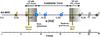 |
Fig. 15 Liquid water habitable zone of GJ 667C with the proposed seven candidates as estimated using the updated relations in Kopparapu et al. (2013). Three of the reported planets lie within the HZ. The newly reported planets f and e are the most comfortably located within it. The inner edge is set by the moist greenhouse runaway limit and the outer edge is set by the snow ball runaway limit. The empirical limits set by a recent uninhabitable Venus and an early habitable Mars are marked in brown solid lines. The presence of clouds of water (inner edge) or CO2 (outer edge) might allow habitable conditions on planets slightly outside the nominal definition of the habitable zone (Selsis et al. 2007). |
After tidal locking, the planet would still have about 0.14 W m-2 of tidal heating due to the eccentricity (which, as for the other candidates, can oscillate between 0 and 0.1 due to dynamical interactions). If we assume an Earth-like planet, then about 90% of that heat is generated in the oceans, and 10% in the rocky interior. Such a planet would have churning oceans, and about 0.01 W m-2 of tidal heat flux from the rocky interior. This number should be compared to 0.08 W m-2, the heat flux on the Earth due entirely to other sources. As e = 0.1 is near the maximum of the secular cycle, see Sect. 8, the actual heat flux is probably much lower. We conclude that tidal heating on planet h is likely to be negligible, with the possibility it could be a minor contributor to the internal energy budget. As the other planets are more distant, the tidal heating of those planets is negligible. The CPL predicts higher heating rates and planet c could receive ~0.01 W m-2 of internal heating, but otherwise tidal heating does not affect the HZ planets.
9.5. The Weather Forecast
Assuming planets c, f and e have habitable surfaces (see Fig. 15), what might their climates be like? To first order we expect a planet’s surface temperature to be cooler as semi-major axis increases because the incident flux falls off with distance squared. However, albedo variations can supersede this trend, e.g. a closer, high-albedo planet could absorb less energy than a more distant low-albedo planet. Furthermore, molecules in the atmosphere can trap photons near the surface via the greenhouse effect, or scatter stellar light via Rayleigh scattering, an anti-greenhouse effect. For example, the equilibrium temperature of Venus is actually lower than the Earth’s due to the former’s large albedo, yet the surface temperature of Venus is much larger than the Earth’s due to the greenhouse effect. Here, we speculate on the climates of each HZ planet based on the our current understanding of the range of possible climates that HZ planets might have.
Certain aspects of each planet will be determined by the redder spectral energy distribution of the host star. For example, the “stratosphere” is expected to be isothermal as there is negligible UV radiation (Segura et al. 2003). On Earth, the UV light absorbed by ozone creates a temperature inversion that delineates the stratosphere. HZ calculations also assume the albedo of planets orbiting cooler stars are lower than the Earth’s because Rayleigh scattering is less effective for longer wavelengths, and because the peak emission in the stellar spectrum is close to several H2O and CO2 absorption bands in the near infrared. Therefore, relative to the Earth’s insolation, the HZ is farther from the star. In other words, if we placed the Earth in orbit around an M dwarf such that it received the same incident radiation as the modern Earth, the M dwarf planet would be hotter as it would have a lower albedo. The different character of the light can also impact plant life, and we might expect less productive photosynthesis (Kiang et al. 2007), perhaps relying on pigments such as chlorophyll d (Mielke et al. 2013) or chlorophyll f (Chen et al. 2010).
Planet c is slightly closer to the inner edge of the HZ than the Earth, and so we expect it to be warmer than the Earth, too. It receives 1230 W m-2 of stellar radiation, which is actually less than the Earth’s solar constant of 1360 W m-2. Assuming synchronous rotation and no obliquity, then the global climate depends strongly on the properties of the atmosphere. If the atmosphere is thin, then the heat absorbed at the substellar point cannot be easily transported to the dark side or the poles. The surface temperature would be a strong function of the zenith angle of the host star GJ 667C. For thicker atmospheres, heat redistribution becomes more significant. With a rotation period of ~28 days, the planet is likely to have Hadley cells that extend to the poles (at least if Titan, with a similar rotation period, is a guide), and hence jet streams and deserts would be unlikely. The location of land masses is also important. Should land be concentrated near the substellar point, then silicate weathering is more effective, and cools the planet by drawing down CO2 (Edson et al. 2012).
Planet f is a prime candidate for habitability and receives 788 W m-2 of radiation. It likely absorbs less energy than the Earth, and hence habitability requires more greenhouse gases, like CO2 or CH4. Therefore a habitable version of this planet has to have a thicker atmosphere than the Earth, and we can assume a relatively uniform surface temperature. Another possibility is an “eyeball” world in which the planet is synchronously rotating and ice-covered except for open ocean at the substellar point (Pierrehumbert 2011). On the other hand, the lower albedo of ice in the IR may make near-global ice coverage difficult (Joshi & Haberle 2012; Shields et al. 2013).
Planet e receives only a third the radiation the Earth does, and lies close to the maximum greenhouse limit. We therefore expect a habitable version of this planet to have >2 bars of CO2. The planet might not be tidally locked, and may have an obliquity that evolves significantly due to perturbations from other planets. From this perspective planet e might be the most Earth-like, experiencing a day-night cycle and seasons.
Finally planet d is unlikely to be in the habitable zone, but it could potentially support subsurface life. Internal energy generated by, e.g., radiogenic heat could support liquid water below an ice layer, similar to Europa. Presumably the biologically generated gases could find their way through the ice and become detectable bio-signatures, but they might be a very small constituent of a large atmosphere, hampering remote detection. While its transit probability is rather low (~0.5%), its apparent angular separation from the star is ~40 milliarcseconds. This value is the baseline inner working angle for the Darwin/ESA high-contrast mission being considered by ESA (Cockell et al. 2009) so planet d could be a primary target for such a mission.
9.6. Moons in the habitable zone of GJ 667C
In addition to planets, extrasolar moons have been suggested as hosts for life (Reynolds et al. 1987; Williams et al. 1997; Tinney et al. 2011; Heller & Barnes 2013). In order to sustain a substantial, long-lived atmosphere under an Earth-like amount of stellar irradiation (Williams et al. 1997; Kaltenegger 2000), to drive a magnetic field over billions of years (Tachinami et al. 2011), and to drive tectonic activity, Heller & Barnes (2013) concluded that a satellite in the stellar HZ needs a mass ≳0.25 M⊕ in order to maintain liquid surface water.
If potential moons around planets GJ 667C c, f, or e formed in the circumplanetary disk, then they will be much less massive than the most massive satellites in the solar system (Canup & Ward 2006) and thus not be habitable. However, if one of those planets is indeed terrestrial then impacts could have created a massive moon as happened on Earth (Cameron & Ward 1976). Further possibilities for the formation of massive satellites are summarized in Heller & Barnes (2013, Sect. 2.1).
As the stellar HZ of GJ 667C is very close to this M dwarf star, moons of planets in the habitable zone would have slightly eccentric orbits due to stellar perturbations. These perturbations induce tidal heating and they could be strong enough to prevent any moon from being habitable (Heller 2012). Moons around planet d, which orbits slightly outside the stellar HZ, could offer a more benign environment to life than the planet itself, if they experience weak tidal heating of, say, a few watts per square meter (see Jupiter’s moon Io, Reynolds et al. 1987; Spencer et al. 2000).
Unless some of these planets are found to transit, there is no currently available technique to identify satellites (Kipping 2009; Kipping et al. 2012). The RV technique is only sensitive to the combined mass of a planet plus its satellites so it might be possible that some of the planets could be somewhat lighter- but host a massive moon.
10. Conclusions
We describe and report the statistical methods and tests used to detect up to seven planet candidates around GJ 667C using Doppler spectroscopy. The detection of the first five planets is very robust and independent of any prior choice. In addition to the first two already reported ones (b and c Anglada-Escudé & Butler 2012; Delfosse et al. 2013) we show that the third planet also proposed in those papers (planet d) is much better explained by a Keplerian orbit rather than an activity-induced periodicity. The next two confidently detected signals (e and f) both correspond to small super-Earth mass objects with most likely periods of 62 and 39 days. The detection of the 6th planet is weakly dependent on the prior choice of the orbital eccentricity. The statistical evidence for the 7th candidate (planet h) is tentative and requires further Doppler follow-up for confirmation. Gregory (2012) proposed a solution for the system with similar characteristics to the one we present here but had fundamental differences. In particular, he also identified the first five stronger signals but his six-planet solution also included a candidate periodicity at 30 days- which would be dynamically unstable- and activity was associated to the signal at 53 days without further discussion or verification. The difference in our conclusions are due to a slightly different choice of priors (especially on the eccentricity), more data was used in our analysis – only HARPS-CCF data was used by Gregory (2012) – , and we performed a more thorough investigation of possible activity-related periodicities.
Numerical integration of orbits compatible with the posterior density distributions show that there is a subset of configurations that allow long-term stable configurations. Except for planets b and g, the condition of dynamical stability dramatically affects the distribution of allowed eccentricities indicating that the lower mass planet candidates (c, e, f) must have quasi-circular orbits. A system of six planets is rather complex in terms of stabilizing mechanisms and possible mean-motion resonances. Nonetheless, we identified that the physically allowed configurations are those that avoid transient 3:1 MMR between planets d and g. We also found that the most stable orbital solutions are described well by the theory of secular frequencies (Laplace-Lagrange solution). We investigated if the inclusion of a seventh planet system was dynamically feasible in the region disclosed by the Bayesian samplings. It is notable that this preliminary candidate appears around the center of the region of stability. Additional data should be able to confirm this signal and provide detectability for longer period signals.
The closely packed dynamics keeps the eccentricities small but non-negligible for the lifetime of the system. As a result, potential habitability of the candidates must account for tidal dissipation effects among others. Dynamics essentially affect 1) the total energy budget at the surface of the planet (tidal heating); 2) synchronization of the rotation with the orbit (tidal locking); and 3) the timescales for the erosion of their obliquities. These dynamical constraints, as well as predictions for potentially habitable super-Earths around M dwarf stars, suggest that at least three planet candidates (planets c, e and f) could have remained habitable for the current life-span of the star. Assuming a rocky composition, planet d lies slightly outside the cold edge of the stellar HZ. Still, given the uncertainties in the planet parameters and in the assumptions in the climatic models, its potential habitability cannot be ruled out (e.g., ocean of liquid water under a thick ice crust, or presence of some strong green-house effect gas).
One of the main results of the Kepler mission is that high-multiplicity systems of dynamically-packed super-Earths are quite common around G and K dwarfs (Fabrycky et al. 2012). The putative existence of these kinds of compact systems around M-dwarfs, combined with a closer-in habitable zone, suggests the existence of a numerous population of planetary systems with several potentially-habitable worlds each. GJ 667C is likely to be among first of many of such systems that may be discovered in the coming years.
Online material
Appendix A: Priors
The choice of uninformative and adequate priors plays a central role in Bayesian
statistics. More classic methods, such as weighted least-squares solvers, can be derived
from Bayes theorem by assuming uniform prior distributions for all free parameters.
Using the definition of Eq. (3), one can
note that, under coordinate transformations in the parameter space (e.g., change from
P to P-1 as the free parameter) the
posterior probability distribution will change its shape through the Jacobian
determinant of this transformation. This means that the posterior distributions are
substantially different under changes of parameterizations and, even in the case of
least-square statistics, one must be very aware of the prior choices made (explicit, or
implicit through the choice of parameterization). This discussion is addressed in more
detail in Tuomi & Anglada-Escudé (2013).
For the Doppler data of GJ 667C, our reference prior choices are summarized in Table
A.1. The basic rationale on each prior choice
can also be found in Tuomi (2012), Anglada-Escudé & Tuomi (2012) and Tuomi & Anglada-Escudé (2013). The prior
choice for the eccentricity can be decisive in detection of weak signals. Our choice for
this prior ( ) is justified using
statistical, dynamical and population arguments.
) is justified using
statistical, dynamical and population arguments.
Appendix A.1: Eccentricity prior: statistical argument
Our first argument is based on statistical considerations to minimize the risk of false positives. That is, since e is a strongly nonlinear parameter in the Keplerian model of Doppler signals (especially if e > 0.5), the likelihood function has many local maxima with high eccentricities. Although such solutions might appear very significant, it can be shown that, when the detected amplitudes approach the uncertainty in the measurements, these high-eccentricity solutions are mostly spurious.
To illustrate this, we generate simulated sets of observations (same observing epochs, no signal, Gaussian white noise injected, 1 m s-1 jitter level), and search for the maximum likelihood solution using the log-L periodograms approach (assuming a fully Keplerian solution at the period search level, see Sect. 4.2). Although no signal is injected, solutions with a formal false-alarm probability (FAP) smaller than 1% are found in 20% of the sample. On the contrary, our log-L periodogram search for circular orbits found 1.2% of false positives, matching the expectations given the imposed 1% threshold. We performed an additional test to assess the impact of the eccentricity prior on the detection completeness. That is, we injected one Keplerian signal (e = 0.8) at the same observing epochs with amplitudes of 1.0 m s-1 and white Gaussian noise of 1 m s-1. We then performed the log-L periodogram search on a large number of these datasets (103). When the search model was allowed to be a fully Keplerian orbit, the correct solution was only recovered 2.5% of the time, and no signals at the right period were spotted assuming a circular orbit. With a K = 2.0 m s-1, the situation improved and 60% of the orbits were identified in the full Keplerian case, against 40% of them in the purely circular one. More tests are illustrated in the left panel of Fig. A.1. When an eccentricity of 0.4 and K = 1 m s-1 signal was injected, the completeness of the fully Keplerian search increased to 91% and the completeness of the circular orbit search increased to 80%. When a K > 2 m s-1 signal was injected, the orbits were identified in >99% of the cases. We also obtained a histogram of the semi-amplitudes of the false positive detections obtained when no signal was injected. The histogram shows that these amplitudes were smaller than 1.0 m s-1 with a 99% confidence level (see right panel of Fig. A.1). This illustrates that statistical tests based on point estimates below the noise level do not produce reliable assessments on the significance of a fully Keplerian signal. For a given dataset, information based on simulations (e.g., Fig. A.1) or a physically motivated prior is necessary to correct such detection bias (Zakamska et al. 2011).
Reference prior probability densities and ranges of the model parameters.
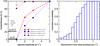 |
Fig. A.1 Left panel. Detection completeness as a function of the injected signal using a fully Keplerian search versus a circular orbit search. Red and blue lines are for an injected eccentricity of 0.8, and the brown and purple ones are for injected signals with eccentricity of 0.4. Black horizontal lines on the left show the fraction of false-positive detections satisfying the FAP threshold of 1% using both methods (Keplerian versus circular). While the completeness is slightly enhanced in the low K regime, the fraction of false positives is unacceptable and, therefore, the implicit assumptions of the method (e.g., uniform prior for e) are not correct. Right panel. Distribution of semi-amplitudes K for these false positive detections. Given that the injected noise level is 1.4 m s-1 (1 m s-1 nominal uncertainty, 1 m s-1 jitter), it is clear that signals detected with fully Keplerian log-L periodograms with K below the noise level cannot be trusted. |
In summary, while a uniform prior on eccentricity only looses a few very eccentric solutions in the low amplitude regime, the rate of false positive detections (~20%) is unacceptable. On the other hand, only a small fraction of highly eccentric orbits are missed if the search is done assuming strictly circular orbits. This implies that, for log-likelihood periodogram searches, circular orbits should always be assumed when searching for a new low-amplitude signals and that, when approaching amplitudes comparable to the measurement uncertainties, assuming circular orbits is a reasonable strategy to avoid false positives. In a Bayesian sense, this means that we have to be very skeptic of highly eccentric orbits when searching for signals close to the noise level. The natural way to address this self-consistently is by imposing a prior on the eccentricity that suppresses the likelihood of highly eccentric orbits. The log-Likelihood periodograms indicate that the strongest possible prior (force e = 0), already does a very good job so, in general, any function less informative than a delta function (π(e) = δ(0)) and a bit more constraining than a uniform prior (π(e) = 1) can provide a more optimal compromise between sensitivity and robustness. Our particular functional choice of the prior (Gaussian distribution with zero-mean and σ = 0.3) is based on dynamical and population analysis considerations.
Appendix A.2: Eccentricity prior: dynamical argument
From a physical point of view, we expect a priori that eccentricities closer to zero are more probable than those close to unity when multiple planets are involved. That is, when one or two planets are clearly present (e.g. GJ 667Cb and GJ 667Cc are solidly detected even with a flat prior in e), high eccentricities in the remaining lower amplitude candidates would correspond to unstable and therefore physically impossible systems.
Our prior for e takes this feature into account (reducing the likelihood of highly eccentric solutions) but still allows high eccentricities if the data insists so (Tuomi 2012). At the sampling level, the only orbital configurations that we explicitly forbid is that we do not allow solutions with orbital crossings. While a rather weak limitation, this requirement essentially removes all extremely eccentric multiplanet solutions (e > 0.8) from our MCMC samples. This requirement does not, for example, remove orbital configurations with close encounters between planets, and the solutions we receive still have to be analyzed by numerical integration to make sure that they correspond to stable systems. As shown in Sect. 8, posterior numerical integration of the samplings illustrate that our prior function was, after all, rather conservative.
Appendix A.3: Eccentricity prior: population argument
To investigate how realistic our prior choice is compared to the statistical properties of the known exoplanet populations, we obtained the parameters of all planet candidates with Msini smaller than 0.1 Mjup as listed in The Extrasolar Planets Encyclopaedia3 as at 2012 December 1. We then produced a histogram in eccentricity bins of 0.1. The obtained distribution follows very nicely a Gaussian function with zero mean and σe = 0.2, meaning that our prior choice is more uninformative (and therefore, more conservative) than the current distribution of detections. This issue is the central topic of Tuomi & Anglada-Escudé (2013), and a more detailed discussion (plus some illustrative plots) can be found in there.
Appendix B: Detailed Bayesian detection sequences
In this section, we provide a more detailed description of detections of seven signals in the combined HARPS-TERRA, PFS, and HIRES data. We also show that the same seven signals (with some small differences due to aliases) are also detected independently when using HARPS-CCF velocities instead of HARPS TERRA ones. The PFS and HIRES measurements used are again those provided in Anglada-Escudé & Butler (2012).
Appendix B.1: HARPS-CCF, PFS and HIRES
First, we perform a detailed analysis with the CCF values provided by Delfosse et al. (2013) in combination with the PFS and HIRES velocities. When increasing the number of planets, parameter k, in our statistical model, we were able to determine the relative probabilities of models with k = 0,1,2,... rather easily. The parameter spaces of all models could be sampled with our Markov chains relatively rapidly and the parameters of the signals converged to the same periodicities and RV amplitudes regardless of the exact initial states of the parameter vectors.
Unlike in Anglada-Escudé et al. (2012) and Delfosse et al. (2013), we observed immediately that k = 2 was not the number of signals favored by the data. While the obvious signals at 7.2 and 28.1 days were easy to detect using samplings of the parameter space, we also quickly discovered a third signal at a period of 91 days. These signals correspond to the planets GJ 667C b, c, and d of Anglada-Escudé et al. (2012) and Delfosse et al. (2013), respectively, though the orbital period of companion d was found to be 75 days by Anglada-Escudé et al. (2012) and 106 days by Delfosse et al. (2013). The periodograms also show considerable power at 106 days corresponding to the solution of Delfosse et al. (2013). Again, it did not provide a solution as probable as the signal at 91 days and the inclusion of linear correlation terms with activity did not affect its significance (see also Sect. 6).
Relative posterior probabilities and log-Bayes factors of models ℳk with k Keplerian signals derived from the combined HARPS-CCF, HIRES, and PFS RV data on the left and HARPS-TERRA HIRES, PFS on the right.
Seven-Keplerian solution of the combined RVs of GJ 667C with HARPS-CCF data.
We could identify three more signals in the data at 39, 53, and 260 days with low RV amplitudes of 1.31, 0.96, and 0.97 ms-1, respectively. The 53-day signal had a strong alias at 62 days and so we treated these as alternative models and calculated their probabilities as well. The inclusion of k = 6 and k = 7 signals at 260 and 17 days improved the models irrespective of the preferred choice of the period of planet e (see Table B.1). To assess the robustness of the detection of the 7-th signal, we started alternative chains at random periods. All the chains that show good signs of convergence (bound period) unequivocally suggested 17 days for the last candidate. Since all these signals satisfied our Bayesian detection criteria, we denoted all of them to planet candidates.
We performed samplings of the parameter space of the model with k = 8 but could not spot a clear 8-th periodicity. The period of such 8th signal converged to a broad probability maximum between 1200 and 2000 days but the corresponding RV amplitude received a posterior density that did not differ significantly from zero. The probability of the model with k = 8 only exceeded the probability of k = 7 by a factor of 60.
We therefore conclude that the combined data set with HARPS-CCF RVs was in favor of k = 7. The corresponding orbital parameters of these seven Keplerian signals are shown in Table B.2. Whether there is a weak signal at roughly 1200–2000 days or not remains to be seen when future data become available. The naming of the seven candidate planets (b to h) follows the significance of detection.
Appendix B.2: HARPS-TERRA, PFS and HIRES (reference solution)
The HARPS-TERRA velocities combined with PFS and HIRES velocities contained the signals of GJ 667C b, c, and d very clearly. We could extract these signals from the data with ease and obtained estimates for orbital periods that were consistent with the estimates obtained using the CCF data in the previous subsection. Unlike for the HARPS-CCF data, however, the 91 day signal was more significantly present in the HARPS-TERRA data and it corresponded to the second most significant periodicity instead of the 28 day one. Also, increasing k improved the statistical model significantly and we could again detect all the additional signals in the RVs.
As for the CCF data, we branched the best fit solution into the two preferred periods for the planet e (53/62 days). The solution and model probabilities are listed on the right-side of Table B.1. The only significant difference compared to the HARPS-CCF one is that the 62-day period for planet e is now preferred. Still, the model with 53 days is only seventeen times less probable than the one with a 62 days signal, so we cannot confidently rule out that the 53 days one is the real one. For simplicity and to avoid confusion, we use the 62-day signal in our reference solution and is the one used to analyze dynamical stability and habitability for the system. As an additional check, preliminary dynamical analysis of solutions with a period of 53 days for planet e showed very similar behavior to the reference solution in terms of long-term stability (similar fraction of dynamically stable orbits and similar distribution for the D chaos indices). Finally, we made several efforts at sampling the eight-Keplerian model with different initial states. As for the CCF data, there are hints of a signal in the ~2000 day period domain that could not be constrained.
Appendix C: Further activity-related tests
Appendix C.1: Correlated noise
The possible effect of correlated noise must be investigated together with the significance of the reported detections (e.g. GJ 581; Baluev 2012; Tuomi & Jenkins 2012). We studied the impact of correlated noise by adding a first order Moving Average term (MA(1), see Tuomi et al. 2013a) to the model in Eq. (1) and repeated the Bayesian search for all the signals. The MA(1) model proposed in (Tuomi et al. 2013a) contains two free parameters: a characteristic time-scale τ and a correlation coefficient c. Even for the HARPS data set with the greatest number of measurements, the characteristic time-scale could not be constrained. Similarly, the correlation coefficient (see e.g. Tuomi et al. 2013b,a) had a posteriori density that was not different from its prior, i.e. it was found to be roughly uniform in the interval [–1,1], which is a natural range for this parameter because it makes the corresponding MA model stationary. While the k = 7 searches lead to the same seven planet solution, models containing such noise terms produced lower integrated probabilities, which suggests over-parameterization. When this happens, one should use the simplest model (principle of parsimony) and accept that the noise is better explained by the white noise components only. Finally, very low levels of correlated noise are also consistent with the good match between synthetic and real periodograms of subsamples in Sect. 7.
Appendix C.2: Including activity correlation in the model
Because the HARPS activity-indices (S-index, FWHM, and BIS) were available, we analyzed the data by taking into account possible correlations with any of these indices. We added an extra component into the statistical model taking into account linear correlation with each of these parameters as F(ti,C) = C zi (see Eq. (1)), where zi is the any of the three indices at epoch ti.
In Sect. 6, we found that the log-L of the solution for planet d slightly improved when adding the correlation term. The slight improvement of the likelihood is compatible with a consistently positive estimate of C for both FWHM and the S-index obtained with the MC samplings (see Fig. C.1, for an example distribution of CS−index as obtained with a k = 3 model). While the correlation terms were observed to be mostly positive in all cases, the 0 value for the coefficient was always within the 95% credibility interval. Moreover, we found that the integrated model probabilities decreased when compared to the model with the same number of planets but no correlation term included. This means that such models are over-parameterized and, therefore, they are penalized by the principle of parsimony.
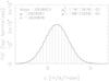 |
Fig. C.1 Value of the linear correlation parameter of the S-index (CS) with the radial velocity data for a model with k = 3 Keplerians (detection of planet d). |
Appendix C.3: Wavelength dependence of the signals
Stellar activity might cause spurious Doppler variability that is wavelength dependent (e.g., cool spots). Using the HARPS-TERRA software on the HARPS spectra only, we extracted one time-series for each echelle aperture (72 of them). This process results is Nobs = 72 × 173 = 12 456 almost independent RV measurements with corresponding uncertainties. Except for calibration related systematic effects (unknown at this level of precision), each echelle aperture can be treated as an independent instrument. Therefore, the reference velocities γl and jitter terms σl of each aperture were considered as free parameters. To assess the wavelength dependence of each signal, the Keplerian model of the i-th planet (one planet at a time) also contained one semi-amplitude Ki,l per echelle aperture and all the other parameters (ei, ωi, M0,i and Pi) were common to all apertures. The resulting statistical model has 72 × 3 + 5 × k − 1 parameters when k Keplerian signals are included and one is investigated (250 free parameters for k = 7). We started the posterior samplings in the vicinity of the solutions of interest because searching the period space would have been computationally too demanding. Neglecting the searches for periodicities, we could obtain relatively well converged samples from the posterior densities in a reasonable time-scale (few days of computer time).
The result is the semi-amplitude K of each signal measured as a function of wavelength. Plotting this K against central wavelength of each echelle order enabled us to visually assess if signals had strong wavelength dependencies (i.e. whether there were signals only present in a few echelle orders) and check if the obtained solution was consistent with the one derived from the combined Doppler measurements. By visual inspection and applying basic statistical tests, we observed that the scatter in the amplitudes for all the candidates was consistent within the error bars and no significant systematic trend (e.g. increasing K towards the blue or the red) was found in any case. Also, the weighted means of the derived amplitudes were fully consistent with the values in Table 4. We are developing a more quantitative version of these tests by studying reported activity-induced signals on a larger sample of stars. As examples of low–amplitude wavelength-dependent signals ruled out using similar tests in the HARPS wavelength range see: Tuomi et al. (2013b) on HD 40307 (K3V), Anglada-Escudé & Butler (2012) on HD 69830 (G8V) and Reiners et al. (2013) on the very active M dwarf AD Leo (M3V).
Publicly available at http://janus.astro.umd.edu/HNBody/
Note that evolution for the CPL model is faster with our parameterization. In the case of GJ 581 d, shown in Heller et al. (2011), the planet was assumed to be less dissipative in the CPL model (Qp = 100) and evolution in the CPL model was slower.
Acknowledgments
We acknowledge the constructive discussions with the referees of this manuscript. The robustness and confidence of the result greatly improved thanks to such discussions. G. Anglada-Escudé is supported by the German Federal Ministry of Education and Research under 05A11MG3. M. Tuomi acknowledges D. Pinfield and RoPACS (Rocky Planets Around Cool Stars), a Marie Curie Initial Training Network funded by the European Commission’s Seventh Framework Programme. E. Gerlach would like to acknowledge the financial support from the DFG research unit FOR584. R. Barnes is supported by NASA’s Virtual Planetary Laboratory under Cooperative Agreement Number NNH05ZDA001C and NSF grant AST-1108882. R. Heller receives funding from the Deutsche Forschungsgemeinschaft (reference number scho394/29-1). J.S. Jenkins also acknowledges funding by Fondecyt through grant 3110004 and partial support from CATA (PB06, Conicyt), the GEMINI-CONICYT FUND and from the Comité Mixto ESO-GOBIERNO DE CHILE. S. Weende acknowledges DFG funding by SFB-963 and the GrK-1351 A. Reiners acknowledges research funding from DFG grant RE1664/9-1. S.S. Vogt gratefully acknowledges support from NSF grant AST-0307493. This study contains data obtained from the ESO Science Archive Facility under request number ANGLADA36104. We also acknowledge the efforts of the PFS/Magellan team in obtaining Doppler measurements. We thank Sandy Keiser for her efficient setup of the computer network at Carnegie/DTM. We thank Dan Fabrycky, Aviv Ofir, Mathias Zechmeister and Denis Shulyak for useful and constructive discussions. This research made use of the Magny Cours Cluster hosted by the GWDG, which is managed by Georg August University Göttingen and the Max Planck Society. This research has made extensive use of the SIMBAD database, operated at CDS, Strasbourg, France; and NASA’s Astrophysics Data System. The authors acknowledge the significant efforts of the HARPS-ESO team in improving the instrument and its data reduction software that made this work possible. We also acknowledge the efforts of the teams and individual observers that have been involved in observing the target star with HARPS/ESO, HIRES/Keck, PFS/Magellan and UVES/ESO.
References
- Abe, Y., Abe-Ouchi, A., Sleep, N. H., & Zahnle, K. J. 2011, Astrobiology, 11, 443 [NASA ADS] [CrossRef] [Google Scholar]
- Anglada-Escudé, G., & Butler, R. P. 2012, ApJS, 200, 15 [NASA ADS] [CrossRef] [Google Scholar]
- Anglada-Escudé, G., & Tuomi, M. 2012, A&A, 548, A58 [NASA ADS] [CrossRef] [EDP Sciences] [Google Scholar]
- Anglada-Escudé, G., López-Morales, M., & Chambers, J. E. 2010, ApJ, 709, 168 [NASA ADS] [CrossRef] [Google Scholar]
- Anglada-Escudé, G., Arriagada, P., Vogt, S. S., et al. 2012, ApJ, 751, L16 [NASA ADS] [CrossRef] [Google Scholar]
- Baliunas, S. L., Donahue, R. A., Soon, W. H., et al. 1995, ApJ, 438, 269 [NASA ADS] [CrossRef] [Google Scholar]
- Baluev, R. V. 2009, MNRAS, 393, 969 [NASA ADS] [CrossRef] [Google Scholar]
- Baluev, R. V. 2012, MNRAS, 420 [Google Scholar]
- Barnes, R., Raymond, S. N., Jackson, B., & Greenberg, R. 2008, Astrobiology, 8, 557 [NASA ADS] [CrossRef] [PubMed] [Google Scholar]
- Barnes, R., Jackson, B., Greenberg, R., & Raymond, S. N. 2009, ApJ., 700, L30 [NASA ADS] [CrossRef] [Google Scholar]
- Barnes, R., Mullins, K., Goldblatt, C., et al. 2013, Astrobiology, 13, 225 [NASA ADS] [CrossRef] [Google Scholar]
- Batalha, N. M., Borucki, W. J., Bryson, S. T., et al. 2011, ApJ, 729, 27 [NASA ADS] [CrossRef] [Google Scholar]
- Bond, J. C., O’Brien, D. P., & Lauretta, D. S. 2010, ApJ, 715, 1050 [NASA ADS] [CrossRef] [Google Scholar]
- Bonfils, X. 2009, in ESO-CAUP Conf. Ser., ed. N. Santos, 1 [Google Scholar]
- Bonfils, X., Delfosse, X., Udry, S., et al. 2013, A&A, 549, A109 [NASA ADS] [CrossRef] [EDP Sciences] [Google Scholar]
- Cameron, A. G. W., & Ward, W. R. 1976, in LPI Science Conf. Abstracts, 7, 120 [Google Scholar]
- Canup, R. M., & Ward, W. R. 2006, Nature, 441, 834 [NASA ADS] [CrossRef] [Google Scholar]
- Carter-Bond, J. C., O’Brien, D. P., & Raymond, S. N. 2012, ApJ, 760, 44 [NASA ADS] [CrossRef] [Google Scholar]
- Cayrel de Strobel, G. 1981, Bulletin d’Information du Centre de Données Stellaires, 20, 28 [NASA ADS] [Google Scholar]
- Chambers, J. E., Wetherill, G. W., & Boss, A. P. 1996, Icarus, 119, 261 [NASA ADS] [CrossRef] [MathSciNet] [Google Scholar]
- Charbonneau, D., Berta, Z. K., Irwin, J., et al. 2009, Nature, 462, 891 [NASA ADS] [CrossRef] [PubMed] [Google Scholar]
- Chen, M., Schliep, M., Willows, R. D., et al. 2010, Science, 329, 1318 [NASA ADS] [CrossRef] [Google Scholar]
- Cockell, C. S., Léger, A., Fridlund, M., et al. 2009, Astrobiology, 9, 1 [NASA ADS] [CrossRef] [PubMed] [Google Scholar]
- Correia, A. C. M., Levrard, B., & Laskar, J. 2008, A&A, 488, L63 [NASA ADS] [CrossRef] [EDP Sciences] [Google Scholar]
- Darwin, G. H. 1880, Roy. Soc. Lond. Philosoph. Trans. Ser. I, 171, 713 [Google Scholar]
- Dawson, R. I., & Fabrycky, D. C. 2010, ApJ, 722, 937 [NASA ADS] [CrossRef] [Google Scholar]
- Delfosse, X., Forveille, T., Ségransan, D., et al. 2000, A&A, 364, 217 [NASA ADS] [Google Scholar]
- Delfosse, X., Bonfils, X., Forveille, T., et al. 2013, A&A, 553, A8 [NASA ADS] [CrossRef] [EDP Sciences] [Google Scholar]
- Dole, S. H. 1964, Habitable planets for man (Blaisdell Pub. Co.) [Google Scholar]
- Edmunds, M. G. 1978, A&A, 64, 103 [NASA ADS] [Google Scholar]
- Edson, A., Lee, S., Bannon, P., Kasting, J. F., & Pollard, D. 2011, Icarus, 212, 1 [NASA ADS] [CrossRef] [Google Scholar]
- Edson, A. R., Kasting, J. F., Pollard, D., Lee, S., & Bannon, P. R. 2012, Astrobiology, 12, 562 [NASA ADS] [CrossRef] [Google Scholar]
- Fabrycky, D. C., Lissauer, J. J., Ragozzine, D., et al. 2012 [arXiv:1202.6328] [Google Scholar]
- Ferraz-Mello, S., Micchtchenko, T. A., & Beaugé, C. 2006, Regular motions in extra-solar planetary systems (Springer), 255 [Google Scholar]
- Ferraz-Mello, S., Rodríguez, A., & Hussmann, H. 2008, Celest. Mech. Dyn. Astron., 101, 171 [Google Scholar]
- Ford, E. B. 2005, AJ, 129, 1706 [Google Scholar]
- Forveille, T., Bonfils, X., Lo Curto, G., et al. 2011, A&A, 526, A141 [NASA ADS] [CrossRef] [EDP Sciences] [Google Scholar]
- Geballe, T. R., Knapp, G. R., Leggett, S. K., et al. 2002, ApJ, 564, 466 [NASA ADS] [CrossRef] [Google Scholar]
- Goldreich, P. 1966, AJ, 71, 1 [NASA ADS] [CrossRef] [Google Scholar]
- Gregory, P. C. 2012 [arXiv:1212.4058] [Google Scholar]
- Haario, H., Saksman, E., & Tamminen, J. 2001, Bernouilli, 7, 223 [Google Scholar]
- Hansen, B., & Murray, N. 2013, ApJ, submitted [arXiv:1301.7431] [Google Scholar]
- Hansen, B. M. S., & Murray, N. 2012, ApJ, 751, 158 [Google Scholar]
- Hart, M. H. 1979, Icarus, 37, 351 [NASA ADS] [CrossRef] [Google Scholar]
- Hawley, S. L., & Pettersen, B. R. 1991, ApJ, 378, 725 [NASA ADS] [CrossRef] [Google Scholar]
- Heller, R. 2012, A&A, 545, L8 [NASA ADS] [CrossRef] [EDP Sciences] [Google Scholar]
- Heller, R., & Barnes, R. 2013, Astrobiology, 13, 18 [NASA ADS] [CrossRef] [Google Scholar]
- Heller, R., Leconte, J., & Barnes, R. 2011, A&A, 528, A27 [NASA ADS] [CrossRef] [EDP Sciences] [Google Scholar]
- Husser, T.-O., Wende-von Berg, S., Dreizler, S., et al. 2013, A&A, 553, A6 [NASA ADS] [CrossRef] [EDP Sciences] [Google Scholar]
- Hut, P. 1981, A&A, 99, 126 [NASA ADS] [Google Scholar]
- Ikoma, M., Emori, H., & Nakazawa, K. 2001, ApJ, 553, 999 [NASA ADS] [CrossRef] [Google Scholar]
- Jackson, B., Barnes, R., & Greenberg, R. 2008, MNRAS, 391, 237 [NASA ADS] [CrossRef] [Google Scholar]
- Jenkins, C. R., & Peacock, J. A. 2011, MNRAS, 413, 2895 [Google Scholar]
- Jenkins, J. S., Jones, H. R. A., Tuomi, M., et al. 2013, ApJ, 766, 67 [NASA ADS] [CrossRef] [Google Scholar]
- Joshi, M. 2003, Astrobiology, 3, 415 [NASA ADS] [CrossRef] [Google Scholar]
- Joshi, M. M., & Haberle, R. M. 2012, Astrobiology, 12, 3 [NASA ADS] [CrossRef] [Google Scholar]
- Joshi, M. M., Haberle, R. M., & Reynolds, R. T. 1997, Icarus, 129, 450 [NASA ADS] [CrossRef] [Google Scholar]
- Kaltenegger, L. 2000, in Exploration and Utilisation of the Moon, eds. B. H. Foing, & M. Perry, ESA SP, 462, 199 [Google Scholar]
- Kasting, J. F., Whitmire, D. P., & Reynolds, R. T. 1993, Icarus, 101, 108 [NASA ADS] [CrossRef] [PubMed] [Google Scholar]
- Kiang, N. Y., Segura, A., Tinetti, G., et al. 2007, Astrobiology, 7, 252 [NASA ADS] [CrossRef] [Google Scholar]
- Kipping, D. M. 2009, MNRAS, 392, 181 [NASA ADS] [CrossRef] [Google Scholar]
- Kipping, D. M., Bakos, G. Á., Buchhave, L., Nesvorný, D., & Schmitt, A. 2012, ApJ, 750, 115 [NASA ADS] [CrossRef] [Google Scholar]
- Kopparapu, R. K., Ramirez, R., Kasting, J. F., et al. 2013, ApJ, 765, 131 [NASA ADS] [CrossRef] [Google Scholar]
- Lambeck, K. 1977, Roy. Soc. Lond. Philosoph. Trans. Ser. A, 287, 545 [Google Scholar]
- Laskar, J. 1990, Icarus, 88, 266 [NASA ADS] [CrossRef] [Google Scholar]
- Laskar, J. 1993, Celest. Mech. Dyn. Astron., 56, 191 [Google Scholar]
- Laskar, J., & Robutel, P. 2001, Celest. Mech. Dyn. Astron., 80, 39 [NASA ADS] [CrossRef] [Google Scholar]
- Laughlin, G., & Chambers, J. E. 2001, ApJ, 551, L109 [NASA ADS] [CrossRef] [Google Scholar]
- Leconte, J., Chabrier, G., Baraffe, I., & Levrard, B. 2010, A&A, 516, A64 [NASA ADS] [CrossRef] [EDP Sciences] [Google Scholar]
- Lin, D. N. C., Bodenheimer, P., & Richardson, D. C. 1996, Nature, 380, 606 [NASA ADS] [CrossRef] [Google Scholar]
- Lissauer, J. J. 2007, ApJ, 660, L149 [NASA ADS] [CrossRef] [Google Scholar]
- Lissauer, J. J., Hubickyj, O., D’Angelo, G., & Bodenheimer, P. 2009, Icarus, 199, 338 [NASA ADS] [CrossRef] [Google Scholar]
- Lo Curto, G., Mayor, M., Benz, W., et al. 2010, A&A, 512, A48 [NASA ADS] [CrossRef] [EDP Sciences] [Google Scholar]
- Lovis, C., & Pepe, F. 2007, A&A, 468, 1115 [NASA ADS] [CrossRef] [EDP Sciences] [Google Scholar]
- Lovis, C., Dumusque, X., Santos, N. C., et al. 2011, A&A, submitted [arXiv:1107.5325] [Google Scholar]
- Makarov, V. V., & Efroimsky, M. 2013, ApJ, 764, 27 [NASA ADS] [CrossRef] [Google Scholar]
- Mayor, M., Bonfils, X., Forveille, T., et al. 2009, A&A, 507, 487 [NASA ADS] [CrossRef] [EDP Sciences] [Google Scholar]
- Mermilliod, J.-C. 1986, Catalogue of Eggen’s UBV data [Google Scholar]
- Mielke, S. P., Kiang, N. Y., Blankenship, R. E., & Mauzerall, D. 2013, BBA – Bioenergetics, 1827, 255 [CrossRef] [Google Scholar]
- Murray, C. D., & Dermott, S. F. 1999, Solar system dynamics (Cambridge University Press) [Google Scholar]
- Neron de Surgy, O., & Laskar, J. 1997, A&A, 318, 975 [NASA ADS] [Google Scholar]
- Pepe, F., Mayor, M., Galland, F., & et al. 2002, A&A, 388, 632 [NASA ADS] [CrossRef] [EDP Sciences] [Google Scholar]
- Pierrehumbert, R. T. 2011, ApJ, 726, L8 [NASA ADS] [CrossRef] [Google Scholar]
- Rauch, K. P., & Hamilton, D. P. 2002, in AAS/Division of Dynamical Astronomy Meeting #33, BAAS, 34, 938 [Google Scholar]
- Raymond, S. N., Scalo, J., & Meadows, V. S. 2007, ApJ, 669, 606 [Google Scholar]
- Reiners, A. 2005, Astron. Nachr., 326, 930 [NASA ADS] [CrossRef] [Google Scholar]
- Reiners, A., & Mohanty, S. 2012, ApJ, 746, 43 [NASA ADS] [CrossRef] [Google Scholar]
- Reiners, A., Shulyak, D., Anglada-Escudé, G., et al. 2013, A&A, 552, A103 [NASA ADS] [CrossRef] [EDP Sciences] [Google Scholar]
- Reynolds, R. T., McKay, C. P., & Kasting, J. F. 1987, Adv. Space Res., 7, 125 [Google Scholar]
- Segura, A., Krelove, K., Kasting, J. F., et al. 2003, Astrobiology, 3, 689 [Google Scholar]
- Segura, A., Walkowicz, L. M., Meadows, V., Kasting, J., & Hawley, S. 2010, Astrobiology, 10, 751 [NASA ADS] [CrossRef] [PubMed] [Google Scholar]
- Selsis, F., Kasting, J. F., Levrard, B., et al. 2007, A&A, 476, 1373 [NASA ADS] [CrossRef] [EDP Sciences] [Google Scholar]
- Shields, A. L., Meadows, V. S., Bitz, C. M., et al. 2013 [arXiv:1305.6926] [Google Scholar]
- Skrutskie, M. F., Cutri, R. M., Stiening, R., et al. 2006, AJ, 131, 1163 [NASA ADS] [CrossRef] [Google Scholar]
- Spencer, J. R., Rathbun, J. A., Travis, L. D., et al. 2000, Science, 288, 1198 [NASA ADS] [CrossRef] [PubMed] [Google Scholar]
- Tachinami, C., Senshu, H., & Ida, S. 2011, ApJ, 726, 70 [NASA ADS] [CrossRef] [Google Scholar]
- Tinney, C. G., Wittenmyer, R. A., Butler, R. P., et al. 2011, ApJ, 732, 31 [Google Scholar]
- Tuomi, M. 2011, A&A, 528, L5 [NASA ADS] [CrossRef] [EDP Sciences] [Google Scholar]
- Tuomi, M. 2012, A&A, 543, A52 [NASA ADS] [CrossRef] [EDP Sciences] [Google Scholar]
- Tuomi, M., & Anglada-Escudé, G. 2013, A&A, 553, A17 [NASA ADS] [CrossRef] [EDP Sciences] [Google Scholar]
- Tuomi, M., & Jenkins, J. S. 2012, A&A, submitted [arXiv:1211.1280] [Google Scholar]
- Tuomi, M., Pinfield, D., & Jones, H. R. A. 2011, A&A, 532, A116 [NASA ADS] [CrossRef] [EDP Sciences] [Google Scholar]
- Tuomi, M., Jones, H. R. A., Jenkins, J. S., et al. 2013a, A&A, 551, A79 [NASA ADS] [CrossRef] [EDP Sciences] [Google Scholar]
- Tuomi, M., Anglada-Escudé, G., Gerlach, E., et al. 2013b, A&A, 549, A48 [NASA ADS] [CrossRef] [EDP Sciences] [Google Scholar]
- Udry, S., Bonfils, X., Delfosse, X., et al. 2007, A&A, 469, L43 [NASA ADS] [CrossRef] [EDP Sciences] [Google Scholar]
- van Leeuwen, F. 2007, A&A, 474, 653 [NASA ADS] [CrossRef] [EDP Sciences] [Google Scholar]
- Vogt, S. S., Butler, R. P., Rivera, E. J., et al. 2010, ApJ, 723, 954 [NASA ADS] [CrossRef] [EDP Sciences] [Google Scholar]
- von Braun, K., Boyajian, T. S., Kane, S. R., et al. 2011, ApJ, 729, L26 [NASA ADS] [CrossRef] [Google Scholar]
- Watson, A. J., Donahue, T. M., & Walker, J. C. G. 1981, Icarus, 48, 150 [NASA ADS] [CrossRef] [Google Scholar]
- West, A. A., Hawley, S. L., Bochanski, J. J., et al. 2008, Astron. J., 135, 785 [NASA ADS] [CrossRef] [Google Scholar]
- Williams, D. M., Kasting, J. F., & Wade, R. A. 1997, Nature, 385, 234 [NASA ADS] [CrossRef] [PubMed] [Google Scholar]
- Wordsworth, R. D., Forget, F., Selsis, F., et al. 2011, ApJ, 733, L48 [NASA ADS] [CrossRef] [Google Scholar]
- Yoder, C. F. 1995, in Global Earth Physics: A Handbook of Physical Constants, ed. T. J. Ahrens, 1 [Google Scholar]
- Zakamska, N. L., Pan, M., & Ford, E. B. 2011, MNRAS, 410, 1895 [NASA ADS] [Google Scholar]
- Zechmeister, M., Kürster, M., Endl, M., et al. 2013, A&A, 552, A78 [NASA ADS] [CrossRef] [EDP Sciences] [Google Scholar]
All Tables
Relative posterior probabilities and log-Bayes factors of models ℳk with k Keplerian signals given the combined HARPS-TERRA, HIRES, and PFS RV data of GJ 667C.
Most significant periods as extracted using log -L periodograms on subsamples of the first Nobs measurements.
Fundamental secular frequencies gk, phases φk and corresponding periods of the six-planet solution.
Minimum and maximum values of the semi-major axes and eccentricities during a run of S6 over 10 Myr.
Relative posterior probabilities and log-Bayes factors of models ℳk with k Keplerian signals derived from the combined HARPS-CCF, HIRES, and PFS RV data on the left and HARPS-TERRA HIRES, PFS on the right.
All Figures
|
Fig. 1 Snapshots of the wavelength regions used in the spectral fit to the UVES spectrum of GJ 667C. The observed spectrum is represented in black, the green curves are the parts of the synthetic spectrum used in the fit. The red lines are also from the synthetic spectrum that were not used to avoid contamination by telluric features or because they did not contain relevant spectroscopic information. Unfitted deep sharp lines – especially on panels four and five from the top of the page – are non-removed telluric features. |
| In the text | |
|
Fig. 2 Log-likelihood periodograms for the seven candidate signals sorted by significance. While the first six signals are easily spotted, the seventh is only detected with log-L periodograms if all orbits are assumed to be circular. |
| In the text | |
|
Fig. 3 Marginalized posterior densities for the Doppler semi-amplitudes of the seven reported signals. |
| In the text | |
|
Fig. 4 RV measurements phase-folded to the best period for each planet. Brown circles are HARPS-TERRA velocities, PFS velocities are depicted as blue triangles, and HIRES velocities are green triangles. Red squares are averages on 20 phase bins of the HARPS-TERRA velocities. The black line corresponds to the best circular orbital fit (visualization purposes only). |
| In the text | |
|
Fig. 5 Top two panels. Log-L periodograms for up to 2 signals in the S-index. The most likely periods of the proposed planet candidates are marked as vertical lines. Bottom two panels. Log-L periodograms for up to 2 signals in the FWHM. Given the proximity of these two signals, it is possible that both of them originate from the same feature (active region corotating with the star) that is slowly evolving with time. |
| In the text | |
|
Fig. 6 Log-likelihood periodograms for planet d (91 days) including the correlation term (red dots) compared to the original periodogram without this term (black line). The inclusion of the correlation term increases the contrast between the peaks at 91 and 105 days, favoring the interpretation of the 91 days signals as a genuine planet candidate. |
| In the text | |
|
Fig. 7 Sequence of periodograms obtained from synthetic noiseless data generated on the first 75 epochs. The signals in Table 4 were sequentially injected from top to bottom. The bottom panel is the periodogram to the real dataset after removing the first 7.2 days planet candidate. |
| In the text | |
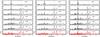 |
Fig. 8 Same as 7 but using the first 100 epochs (left), first 120 (center) and all of them (right). |
| In the text | |
|
Fig. 9 Periodograms on first and second half of the time series as obtained when all signals except one were removed from the data. Except for signal h, all signals are significantly present in both halves and could have been recovered using either half if they had been in single planet systems. |
| In the text | |
|
Fig. 10 Result of the stability analysis of 80 000 six-planet solutions in the plane of initial semi-major axis a vs. initial mean longitude λ obtained from a numerical integration over T ≈ 7000 years. Each initial condition is represented as a point. Initial conditions leading to an immediate disintegration of the system are shown as gray dots. Initial conditions that lead to stable motion for at least 1 Myr are shown as red points (D < 10-5). Black crosses represent the most stable solutions (D < 10-6), and can last over many Myr. |
| In the text | |
|
Fig. 11 Marginalized posterior densities for the orbital eccentricities of the six planet solution (b, c, d, in the first row; e, f, g in the second) before (gray histogram) and after (red histogram) ruling out dynamically unstable configurations. |
| In the text | |
|
Fig. 12 Evolution of the eccentricities of solution S6. Colored lines give the eccentricity as obtained from a numerical integration. The thin black lines show the eccentricity of the respective planet as given by the linear, secular approximation. Close to each line we give the name of the corresponding planet. |
| In the text | |
|
Fig. 13 Stability plot of the possible location of a 7th planet in the stable S6 solution (Table 5). We investigate the stability of an additional planet with 1.1 Earth masses around the location found by the Bayesian analysis. For these integrations, we varied the semi-major axis and eccentricity of the putative planet on a regular grid. The orbital angles ω and M0 were set to the values of the statistically preferred solution, while the inclination was fixed to zero. The nominal positions of the planets as given in Table 6 are marked with white crosses. |
| In the text | |
|
Fig. 14 Tidal evolution of the spin properties of planet GJ 667C f. Solid lines depict predictions from constant-time-lag theory (“CTL”), while dashed lines illustrate those from a constant-phase-lag model (“CPL”). All tracks assume a scenario similar to the “base” configuration (see text and Table 9). Left: despinning for an assumed initial rotation period of one day. The CPL model yields tidal locking in less than 5 Myr, and CTL theory predicts about 20 Myr for tidal locking. Right: tilt erosion of an assumed initial Earth-like obliquity of 23.5°. Time scales for both CPL and CTL models are similar to the locking time scales. |
| In the text | |
|
Fig. 15 Liquid water habitable zone of GJ 667C with the proposed seven candidates as estimated using the updated relations in Kopparapu et al. (2013). Three of the reported planets lie within the HZ. The newly reported planets f and e are the most comfortably located within it. The inner edge is set by the moist greenhouse runaway limit and the outer edge is set by the snow ball runaway limit. The empirical limits set by a recent uninhabitable Venus and an early habitable Mars are marked in brown solid lines. The presence of clouds of water (inner edge) or CO2 (outer edge) might allow habitable conditions on planets slightly outside the nominal definition of the habitable zone (Selsis et al. 2007). |
| In the text | |
|
Fig. A.1 Left panel. Detection completeness as a function of the injected signal using a fully Keplerian search versus a circular orbit search. Red and blue lines are for an injected eccentricity of 0.8, and the brown and purple ones are for injected signals with eccentricity of 0.4. Black horizontal lines on the left show the fraction of false-positive detections satisfying the FAP threshold of 1% using both methods (Keplerian versus circular). While the completeness is slightly enhanced in the low K regime, the fraction of false positives is unacceptable and, therefore, the implicit assumptions of the method (e.g., uniform prior for e) are not correct. Right panel. Distribution of semi-amplitudes K for these false positive detections. Given that the injected noise level is 1.4 m s-1 (1 m s-1 nominal uncertainty, 1 m s-1 jitter), it is clear that signals detected with fully Keplerian log-L periodograms with K below the noise level cannot be trusted. |
| In the text | |
|
Fig. C.1 Value of the linear correlation parameter of the S-index (CS) with the radial velocity data for a model with k = 3 Keplerians (detection of planet d). |
| In the text | |
Current usage metrics show cumulative count of Article Views (full-text article views including HTML views, PDF and ePub downloads, according to the available data) and Abstracts Views on Vision4Press platform.
Data correspond to usage on the plateform after 2015. The current usage metrics is available 48-96 hours after online publication and is updated daily on week days.
Initial download of the metrics may take a while.