| Issue |
A&A
Volume 556, August 2013
|
|
|---|---|---|
| Article Number | A126 | |
| Number of page(s) | 24 | |
| Section | Planets and planetary systems | |
| DOI | https://doi.org/10.1051/0004-6361/201321331 | |
| Published online | 07 August 2013 | |
Online material
Appendix A: Priors
The choice of uninformative and adequate priors plays a central role in Bayesian
statistics. More classic methods, such as weighted least-squares solvers, can be derived
from Bayes theorem by assuming uniform prior distributions for all free parameters.
Using the definition of Eq. (3), one can
note that, under coordinate transformations in the parameter space (e.g., change from
P to P-1 as the free parameter) the
posterior probability distribution will change its shape through the Jacobian
determinant of this transformation. This means that the posterior distributions are
substantially different under changes of parameterizations and, even in the case of
least-square statistics, one must be very aware of the prior choices made (explicit, or
implicit through the choice of parameterization). This discussion is addressed in more
detail in Tuomi & Anglada-Escudé (2013).
For the Doppler data of GJ 667C, our reference prior choices are summarized in Table
A.1. The basic rationale on each prior choice
can also be found in Tuomi (2012), Anglada-Escudé & Tuomi (2012) and Tuomi & Anglada-Escudé (2013). The prior
choice for the eccentricity can be decisive in detection of weak signals. Our choice for
this prior ( ) is justified using
statistical, dynamical and population arguments.
) is justified using
statistical, dynamical and population arguments.
Appendix A.1: Eccentricity prior: statistical argument
Our first argument is based on statistical considerations to minimize the risk of false positives. That is, since e is a strongly nonlinear parameter in the Keplerian model of Doppler signals (especially if e > 0.5), the likelihood function has many local maxima with high eccentricities. Although such solutions might appear very significant, it can be shown that, when the detected amplitudes approach the uncertainty in the measurements, these high-eccentricity solutions are mostly spurious.
To illustrate this, we generate simulated sets of observations (same observing epochs, no signal, Gaussian white noise injected, 1 m s-1 jitter level), and search for the maximum likelihood solution using the log-L periodograms approach (assuming a fully Keplerian solution at the period search level, see Sect. 4.2). Although no signal is injected, solutions with a formal false-alarm probability (FAP) smaller than 1% are found in 20% of the sample. On the contrary, our log-L periodogram search for circular orbits found 1.2% of false positives, matching the expectations given the imposed 1% threshold. We performed an additional test to assess the impact of the eccentricity prior on the detection completeness. That is, we injected one Keplerian signal (e = 0.8) at the same observing epochs with amplitudes of 1.0 m s-1 and white Gaussian noise of 1 m s-1. We then performed the log-L periodogram search on a large number of these datasets (103). When the search model was allowed to be a fully Keplerian orbit, the correct solution was only recovered 2.5% of the time, and no signals at the right period were spotted assuming a circular orbit. With a K = 2.0 m s-1, the situation improved and 60% of the orbits were identified in the full Keplerian case, against 40% of them in the purely circular one. More tests are illustrated in the left panel of Fig. A.1. When an eccentricity of 0.4 and K = 1 m s-1 signal was injected, the completeness of the fully Keplerian search increased to 91% and the completeness of the circular orbit search increased to 80%. When a K > 2 m s-1 signal was injected, the orbits were identified in >99% of the cases. We also obtained a histogram of the semi-amplitudes of the false positive detections obtained when no signal was injected. The histogram shows that these amplitudes were smaller than 1.0 m s-1 with a 99% confidence level (see right panel of Fig. A.1). This illustrates that statistical tests based on point estimates below the noise level do not produce reliable assessments on the significance of a fully Keplerian signal. For a given dataset, information based on simulations (e.g., Fig. A.1) or a physically motivated prior is necessary to correct such detection bias (Zakamska et al. 2011).
Reference prior probability densities and ranges of the model parameters.
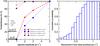 |
Fig. A.1
Left panel. Detection completeness as a function of the injected signal using a fully Keplerian search versus a circular orbit search. Red and blue lines are for an injected eccentricity of 0.8, and the brown and purple ones are for injected signals with eccentricity of 0.4. Black horizontal lines on the left show the fraction of false-positive detections satisfying the FAP threshold of 1% using both methods (Keplerian versus circular). While the completeness is slightly enhanced in the low K regime, the fraction of false positives is unacceptable and, therefore, the implicit assumptions of the method (e.g., uniform prior for e) are not correct. Right panel. Distribution of semi-amplitudes K for these false positive detections. Given that the injected noise level is 1.4 m s-1 (1 m s-1 nominal uncertainty, 1 m s-1 jitter), it is clear that signals detected with fully Keplerian log-L periodograms with K below the noise level cannot be trusted. |
| Open with DEXTER | |
In summary, while a uniform prior on eccentricity only looses a few very eccentric solutions in the low amplitude regime, the rate of false positive detections (~20%) is unacceptable. On the other hand, only a small fraction of highly eccentric orbits are missed if the search is done assuming strictly circular orbits. This implies that, for log-likelihood periodogram searches, circular orbits should always be assumed when searching for a new low-amplitude signals and that, when approaching amplitudes comparable to the measurement uncertainties, assuming circular orbits is a reasonable strategy to avoid false positives. In a Bayesian sense, this means that we have to be very skeptic of highly eccentric orbits when searching for signals close to the noise level. The natural way to address this self-consistently is by imposing a prior on the eccentricity that suppresses the likelihood of highly eccentric orbits. The log-Likelihood periodograms indicate that the strongest possible prior (force e = 0), already does a very good job so, in general, any function less informative than a delta function (π(e) = δ(0)) and a bit more constraining than a uniform prior (π(e) = 1) can provide a more optimal compromise between sensitivity and robustness. Our particular functional choice of the prior (Gaussian distribution with zero-mean and σ = 0.3) is based on dynamical and population analysis considerations.
Appendix A.2: Eccentricity prior: dynamical argument
From a physical point of view, we expect a priori that eccentricities closer to zero are more probable than those close to unity when multiple planets are involved. That is, when one or two planets are clearly present (e.g. GJ 667Cb and GJ 667Cc are solidly detected even with a flat prior in e), high eccentricities in the remaining lower amplitude candidates would correspond to unstable and therefore physically impossible systems.
Our prior for e takes this feature into account (reducing the likelihood of highly eccentric solutions) but still allows high eccentricities if the data insists so (Tuomi 2012). At the sampling level, the only orbital configurations that we explicitly forbid is that we do not allow solutions with orbital crossings. While a rather weak limitation, this requirement essentially removes all extremely eccentric multiplanet solutions (e > 0.8) from our MCMC samples. This requirement does not, for example, remove orbital configurations with close encounters between planets, and the solutions we receive still have to be analyzed by numerical integration to make sure that they correspond to stable systems. As shown in Sect. 8, posterior numerical integration of the samplings illustrate that our prior function was, after all, rather conservative.
Appendix A.3: Eccentricity prior: population argument
To investigate how realistic our prior choice is compared to the statistical properties of the known exoplanet populations, we obtained the parameters of all planet candidates with Msini smaller than 0.1 Mjup as listed in The Extrasolar Planets Encyclopaedia3 as at 2012 December 1. We then produced a histogram in eccentricity bins of 0.1. The obtained distribution follows very nicely a Gaussian function with zero mean and σe = 0.2, meaning that our prior choice is more uninformative (and therefore, more conservative) than the current distribution of detections. This issue is the central topic of Tuomi & Anglada-Escudé (2013), and a more detailed discussion (plus some illustrative plots) can be found in there.
Appendix B: Detailed Bayesian detection sequences
In this section, we provide a more detailed description of detections of seven signals in the combined HARPS-TERRA, PFS, and HIRES data. We also show that the same seven signals (with some small differences due to aliases) are also detected independently when using HARPS-CCF velocities instead of HARPS TERRA ones. The PFS and HIRES measurements used are again those provided in Anglada-Escudé & Butler (2012).
Appendix B.1: HARPS-CCF, PFS and HIRES
First, we perform a detailed analysis with the CCF values provided by Delfosse et al. (2013) in combination with the PFS and HIRES velocities. When increasing the number of planets, parameter k, in our statistical model, we were able to determine the relative probabilities of models with k = 0,1,2,... rather easily. The parameter spaces of all models could be sampled with our Markov chains relatively rapidly and the parameters of the signals converged to the same periodicities and RV amplitudes regardless of the exact initial states of the parameter vectors.
Unlike in Anglada-Escudé et al. (2012) and Delfosse et al. (2013), we observed immediately that k = 2 was not the number of signals favored by the data. While the obvious signals at 7.2 and 28.1 days were easy to detect using samplings of the parameter space, we also quickly discovered a third signal at a period of 91 days. These signals correspond to the planets GJ 667C b, c, and d of Anglada-Escudé et al. (2012) and Delfosse et al. (2013), respectively, though the orbital period of companion d was found to be 75 days by Anglada-Escudé et al. (2012) and 106 days by Delfosse et al. (2013). The periodograms also show considerable power at 106 days corresponding to the solution of Delfosse et al. (2013). Again, it did not provide a solution as probable as the signal at 91 days and the inclusion of linear correlation terms with activity did not affect its significance (see also Sect. 6).
Relative posterior probabilities and log-Bayes factors of models ℳk with k Keplerian signals derived from the combined HARPS-CCF, HIRES, and PFS RV data on the left and HARPS-TERRA HIRES, PFS on the right.
Seven-Keplerian solution of the combined RVs of GJ 667C with HARPS-CCF data.
We could identify three more signals in the data at 39, 53, and 260 days with low RV amplitudes of 1.31, 0.96, and 0.97 ms-1, respectively. The 53-day signal had a strong alias at 62 days and so we treated these as alternative models and calculated their probabilities as well. The inclusion of k = 6 and k = 7 signals at 260 and 17 days improved the models irrespective of the preferred choice of the period of planet e (see Table B.1). To assess the robustness of the detection of the 7-th signal, we started alternative chains at random periods. All the chains that show good signs of convergence (bound period) unequivocally suggested 17 days for the last candidate. Since all these signals satisfied our Bayesian detection criteria, we denoted all of them to planet candidates.
We performed samplings of the parameter space of the model with k = 8 but could not spot a clear 8-th periodicity. The period of such 8th signal converged to a broad probability maximum between 1200 and 2000 days but the corresponding RV amplitude received a posterior density that did not differ significantly from zero. The probability of the model with k = 8 only exceeded the probability of k = 7 by a factor of 60.
We therefore conclude that the combined data set with HARPS-CCF RVs was in favor of k = 7. The corresponding orbital parameters of these seven Keplerian signals are shown in Table B.2. Whether there is a weak signal at roughly 1200–2000 days or not remains to be seen when future data become available. The naming of the seven candidate planets (b to h) follows the significance of detection.
Appendix B.2: HARPS-TERRA, PFS and HIRES (reference solution)
The HARPS-TERRA velocities combined with PFS and HIRES velocities contained the signals of GJ 667C b, c, and d very clearly. We could extract these signals from the data with ease and obtained estimates for orbital periods that were consistent with the estimates obtained using the CCF data in the previous subsection. Unlike for the HARPS-CCF data, however, the 91 day signal was more significantly present in the HARPS-TERRA data and it corresponded to the second most significant periodicity instead of the 28 day one. Also, increasing k improved the statistical model significantly and we could again detect all the additional signals in the RVs.
As for the CCF data, we branched the best fit solution into the two preferred periods for the planet e (53/62 days). The solution and model probabilities are listed on the right-side of Table B.1. The only significant difference compared to the HARPS-CCF one is that the 62-day period for planet e is now preferred. Still, the model with 53 days is only seventeen times less probable than the one with a 62 days signal, so we cannot confidently rule out that the 53 days one is the real one. For simplicity and to avoid confusion, we use the 62-day signal in our reference solution and is the one used to analyze dynamical stability and habitability for the system. As an additional check, preliminary dynamical analysis of solutions with a period of 53 days for planet e showed very similar behavior to the reference solution in terms of long-term stability (similar fraction of dynamically stable orbits and similar distribution for the D chaos indices). Finally, we made several efforts at sampling the eight-Keplerian model with different initial states. As for the CCF data, there are hints of a signal in the ~2000 day period domain that could not be constrained.
Appendix C: Further activity-related tests
Appendix C.1: Correlated noise
The possible effect of correlated noise must be investigated together with the significance of the reported detections (e.g. GJ 581; Baluev 2012; Tuomi & Jenkins 2012). We studied the impact of correlated noise by adding a first order Moving Average term (MA(1), see Tuomi et al. 2013a) to the model in Eq. (1) and repeated the Bayesian search for all the signals. The MA(1) model proposed in (Tuomi et al. 2013a) contains two free parameters: a characteristic time-scale τ and a correlation coefficient c. Even for the HARPS data set with the greatest number of measurements, the characteristic time-scale could not be constrained. Similarly, the correlation coefficient (see e.g. Tuomi et al. 2013b,a) had a posteriori density that was not different from its prior, i.e. it was found to be roughly uniform in the interval [–1,1], which is a natural range for this parameter because it makes the corresponding MA model stationary. While the k = 7 searches lead to the same seven planet solution, models containing such noise terms produced lower integrated probabilities, which suggests over-parameterization. When this happens, one should use the simplest model (principle of parsimony) and accept that the noise is better explained by the white noise components only. Finally, very low levels of correlated noise are also consistent with the good match between synthetic and real periodograms of subsamples in Sect. 7.
Appendix C.2: Including activity correlation in the model
Because the HARPS activity-indices (S-index, FWHM, and BIS) were available, we analyzed the data by taking into account possible correlations with any of these indices. We added an extra component into the statistical model taking into account linear correlation with each of these parameters as F(ti,C) = C zi (see Eq. (1)), where zi is the any of the three indices at epoch ti.
In Sect. 6, we found that the log-L of the solution for planet d slightly improved when adding the correlation term. The slight improvement of the likelihood is compatible with a consistently positive estimate of C for both FWHM and the S-index obtained with the MC samplings (see Fig. C.1, for an example distribution of CS−index as obtained with a k = 3 model). While the correlation terms were observed to be mostly positive in all cases, the 0 value for the coefficient was always within the 95% credibility interval. Moreover, we found that the integrated model probabilities decreased when compared to the model with the same number of planets but no correlation term included. This means that such models are over-parameterized and, therefore, they are penalized by the principle of parsimony.
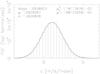 |
Fig. C.1
Value of the linear correlation parameter of the S-index (CS) with the radial velocity data for a model with k = 3 Keplerians (detection of planet d). |
| Open with DEXTER | |
Appendix C.3: Wavelength dependence of the signals
Stellar activity might cause spurious Doppler variability that is wavelength dependent (e.g., cool spots). Using the HARPS-TERRA software on the HARPS spectra only, we extracted one time-series for each echelle aperture (72 of them). This process results is Nobs = 72 × 173 = 12 456 almost independent RV measurements with corresponding uncertainties. Except for calibration related systematic effects (unknown at this level of precision), each echelle aperture can be treated as an independent instrument. Therefore, the reference velocities γl and jitter terms σl of each aperture were considered as free parameters. To assess the wavelength dependence of each signal, the Keplerian model of the i-th planet (one planet at a time) also contained one semi-amplitude Ki,l per echelle aperture and all the other parameters (ei, ωi, M0,i and Pi) were common to all apertures. The resulting statistical model has 72 × 3 + 5 × k − 1 parameters when k Keplerian signals are included and one is investigated (250 free parameters for k = 7). We started the posterior samplings in the vicinity of the solutions of interest because searching the period space would have been computationally too demanding. Neglecting the searches for periodicities, we could obtain relatively well converged samples from the posterior densities in a reasonable time-scale (few days of computer time).
The result is the semi-amplitude K of each signal measured as a function of wavelength. Plotting this K against central wavelength of each echelle order enabled us to visually assess if signals had strong wavelength dependencies (i.e. whether there were signals only present in a few echelle orders) and check if the obtained solution was consistent with the one derived from the combined Doppler measurements. By visual inspection and applying basic statistical tests, we observed that the scatter in the amplitudes for all the candidates was consistent within the error bars and no significant systematic trend (e.g. increasing K towards the blue or the red) was found in any case. Also, the weighted means of the derived amplitudes were fully consistent with the values in Table 4. We are developing a more quantitative version of these tests by studying reported activity-induced signals on a larger sample of stars. As examples of low–amplitude wavelength-dependent signals ruled out using similar tests in the HARPS wavelength range see: Tuomi et al. (2013b) on HD 40307 (K3V), Anglada-Escudé & Butler (2012) on HD 69830 (G8V) and Reiners et al. (2013) on the very active M dwarf AD Leo (M3V).
© ESO, 2013
Current usage metrics show cumulative count of Article Views (full-text article views including HTML views, PDF and ePub downloads, according to the available data) and Abstracts Views on Vision4Press platform.
Data correspond to usage on the plateform after 2015. The current usage metrics is available 48-96 hours after online publication and is updated daily on week days.
Initial download of the metrics may take a while.