| Issue |
A&A
Volume 554, June 2013
|
|
|---|---|---|
| Article Number | A83 | |
| Number of page(s) | 34 | |
| Section | Interstellar and circumstellar matter | |
| DOI | https://doi.org/10.1051/0004-6361/201220976 | |
| Published online | 07 June 2013 | |
Water in star-forming regions with Herschel (WISH)⋆,⋆⋆
IV. A survey of low-J H2O line profiles toward high-mass protostars
1 SRON Netherlands Institute for Space Research, Landleven 12, 9747 AD Groningen, The Netherlands
e-mail: vdtak@sron.nl
2 Kapteyn Astronomical Institute, University of Groningen, The Netherlands
3 Univ. Bordeaux, LAB, 33270 Floirac, France
4 CNRS, LAB, 33271 Floirac, France
5 Centro de Astrobiología (CSIC – INTA), 28850 Madrid, Spain
6 Max-Planck-Institut für Radioastronomie, 53121 Bonn, Germany
7 INAF – Osservatorio Astrofisico di Arcetri, 50125 Firenze, Italy
8 Dublin Institute for Advanced Studies, Dublin 4, Ireland
9 Leiden Observatory, Leiden University, The Netherlands
10 Max-Planck-Institut für Extraterrestrische Physik, 85748 Garching, Germany
11 Institute of Astronomy, ETH Zürich, Switzerland
12 Department of Astronomy, University of Michigan, MI 48109, USA
13 School of Physics and Astronomy, University of Leeds, LS2 9JT, UK
14 Joint Astronomy Center, Hilo, Hawaii, HI 96720, USA
15 Harvard-Smithsonian Center for Astrophysics, Cambridge, MA 02138, USA
16 Onsala Space Observatory, Chalmers University of Technology, 41296 Göteborg, Sweden
17 INAF – Osservatorio Astrofisico di Roma, Italy
18 Observatorio Astronómico Nacional, 28049 Madrid, Spain
Received: 21 December 2012
Accepted: 8 April 2013
Context. Water is a key constituent of star-forming matter, but the origin of its line emission and absorption during high-mass star formation is not well understood.
Aims. We study the velocity profiles of low-excitation H2O lines toward 19 high-mass star-forming regions and search for trends with luminosity, mass, and evolutionary stage.
Methods. We decompose high-resolution Herschel-HIFI line spectra near 990, 1110 and 1670 GHz into three distinct physical components. Dense cores (protostellar envelopes) are usually seen as narrow absorptions in the H2O 1113 and 1669 GHz ground-state lines, the H2O 987 GHz excited-state line, and the H218O 1102 GHz ground-state line. In a few sources, the envelopes appear in emission in some or all studied lines, indicating higher temperatures or densities. Broader features due to outflows are usually seen in absorption in the H2O 1113 and 1669 GHz lines, in 987 GHz emission, and not seen in H218O, indicating a lower column density and a higher excitation temperature than the envelope component. A few outflows are detected in H218O, indicating higher column densities of shocked gas. In addition, the H2O 1113 and 1669 GHz spectra show narrow absorptions by foreground clouds along the line of sight. The lack of corresponding features in the 987 GHz and H218O lines indicates a low column density and a low excitation temperature for these clouds, although their derived H2O ortho/para ratios are close to 3.
Results. The intensity of the ground state lines of H2O at 1113 and 1669 GHz does not show significant trends with source luminosity, envelope mass, or evolutionary state. In contrast, the flux in the excited-state 987 GHz line appears correlated with luminosity and the H218O line flux appears correlated with the envelope mass. Furthermore, appearance of the envelope in absorption in the 987 GHz and H218O lines seems to be a sign of an early evolutionary stage, as probed by the mid-infrared brightness and the Lbol/Menv ratio of the source.
Conclusions. The ground state transitions of H2O trace the outer parts of the envelopes, so that the effects of star formation are mostly noticeable in the outflow wings. These lines are heavily affected by absorption, so that line ratios of H2O involving the ground states must be treated with caution, especially if multiple clouds are superposed as in the extragalactic case. The isotopic H218O line appears to trace the mass of the protostellar envelope, indicating that the average H2O abundance in high-mass protostellar envelopes does not change much with time. The excited state line at 987 GHz increases in flux with luminosity and appears to be a good tracer of the mean weighted dust temperature of the source, which may explain why it is readily seen in distant galaxies.
Key words: stars: formation / ISM: molecules / astrochemistry
Herschel is an ESA space observatory with science instruments provided by European-led Principal Investigator consortia and with important participation from NASA.
Appendices are available in electronic form at http://www.aanda.org
© ESO, 2013
1. Introduction
The water molecule is a key constituent of star-forming matter with a great influence on the formation of stars and planets1. In the gas phase, water acts as a coolant of collapsing dense interstellar clouds; in the solid state, it enhances the coagulation of dust grains in protoplanetary disks to make planetesimals; and as a liquid, it acts as a solvent bringing organic molecules together on planetary surfaces, which is a key step towards biogenic activity. The first role is especially important for high-mass star formation which depends on the balance between the collapse of a massive gas cloud and its fragmentation (Zinnecker & Yorke 2007). This balance depends strongly on the temperature (through the Jeans mass), and the sensitivity of the H2O abundance to the temperature, much larger than for CO, should make it a useful probe of the high-mass star formation process, which is mostly unexplored due to observational difficulties.
Interstellar H2O is well known from ground-based observations of maser emission at centimeter (22 GHz; Cheung et al. 1969), millimeter (183 GHz; Cernicharo et al. 1990), and submillimeter (325 GHz; Menten et al. 1990) wavelengths. The high intrinsic brightness of maser emission makes it useful as a signpost of dense gas and for kinematic studies of protostellar environments (e.g., Trinidad et al. 2003; Sanna et al. 2012a). With VLBI techniques, the proper motions and parallaxes of H2O masers can be measured to micro-arcsecond accuracy, leading to accurate distance estimates for star-forming regions as distant as ~10 kpc (Sanna et al. 2012b) and a revised picture of Galactic structure (Reid et al. 2009).
Source sample.
Thermal H2O lines are useful as probes of physical conditions and the chemical evolution of star-forming regions, but generally cannot be observed from the ground. Before Herschel, space-based submillimeter and far-infrared observations of H2O lines were made with ISO (Van Dishoeck & Helmich 1996), SWAS (Melnick & Bergin 2005) and Odin (Bjerkeli et al. 2009), but these data do not have sufficient angular resolution to determine the spatial distribution of H2O. In contrast, space-based mid-infrared and ground-based mm-wave observations of thermal H2O and H O lines have high angular resolution but only probe the small fraction of the gas at high temperatures (Van der Tak et al. 2006; Watson et al. 2007; Jørgensen & van Dishoeck 2010; Wang et al. 2012).
The first results from the Herschel mission have demonstrated the potential of H2O observations of high-mass star-forming regions at high spatial and spectral resolution. Mapping of the DR21 region shows orders of magnitude variations in H2O abundance between various physical components (envelope, outflow, foreground clouds) due to freeze-out, evaporation, warm gas-phase chemistry, and photodissociation (Van der Tak et al. 2010). Multi-line observations of the high-mass protostar W3 IRS5 show broad emission as well as blueshifted absorption by H2O in the outflow, in particular in lines from excited states of H2O, underlining the importance of shock chemistry for H2O (Chavarría et al. 2010). Observations of the p-H2O and p-HO ground state lines and the p-H2O first excited state line at 987 GHz toward four high-mass star-forming regions indicate H2O abundances ranging from 5 × 10⁻¹⁰ to 4 × 10⁻⁸ without a clear trend with the physical properties of the sources (Marseille et al. 2010b). Finally, observations of multiple H2O, HO and H O lines toward the massive star-forming region NGC 6334I show high-excitation line emission from hot (~200 K) gas, and a H2O abundance ranging from ≈10-8 in cold quiescent gas to 4 × 10⁻⁵ in warm outflow material (Emprechtinger et al. 2010). However, these papers study either single sources or small sets of sources, which makes a trend analysis inconclusive, if not impossible.
This paper presents observations of low-excitation lines of H2O and HO toward 19 regions of high-mass star formation (Table 1). The velocity-resolved spectra show a mixture of emission and absorption due to various physical components, which we disentangle by fitting Gaussian profiles. The resulting line fluxes for the protostellar envelopes and the molecular outflows are compared with basic source parameters such as luminosity and mass, as well as to the evolutionary stage of the source as estimated in various ways.
To probe the bulk of the material in the protostellar environment, this paper focuses on the lowest excitation lines of H2O. The advantage of p-H2O is that its two lowest-excitation lines are close in frequency (Table 2) so that the telescope beam is similar in size. This coincidence allows us to make estimates of the column density and the excitation temperature of H2O which are almost independent of assumptions on the size or the shape of the object. In addition, we use observations of the o-H2O ground-state line at 1669 GHz to probe the kinematics of the sources, which have a high continuum brightness at this high frequency, so that absorption lines are easily detected. This paper does not discuss observations of the other o-H2O ground-state line at 557 GHz, because of the large difference in frequency and beam size. Maps of the 557 GHz line toward our sources will be presented elsewhere.
Table 1 presents the sources, which have been selected from several surveys (Molinari et al. 1996; Sridharan et al. 2002; Wood & Churchwell 1989; Van der Tak et al. 2000), where preference is given to nearby (≲2 kpc) objects and “clean” objects where one source dominates the emission on ≈30′′ scales, which is the relevant scale for our observations. Furthermore, the sources were selected to cover a range of evolutionary stages. In high-mass protostellar objects (HMPOs), the central star is surrounded by a massive envelope with a centrally peaked temperature and density distribution. These objects show signs of active star formation such as outflows and masers. This paper distinguishes mid-IR-bright and -quiet HMPOs, with a boundary of 10 Jy at 12 μm, which may be an evolutionary difference (Van der Tak et al. 2000; Motte et al. 2007; López-Sepulcre et al. 2010). The presence of a “hot core” (submillimeter emission lines from complex organic molecules) or an “ultracompact Hii region” (free-free continuum emission of more than a few mJy at a distance of a few kpc) are thought to be signposts of advanced stages of protostellar evolution. Hot cores occur when a star heats its surroundings such that ice mantles evaporate off dust grains which alters the chemical composition of the circumstellar gas. When the stellar atmosphere becomes hot enough for the production of significant ultraviolet radiation, the circumstellar gas is ionized and an ultracompact Hii region is created.
This paper is organized as follows: Sect. 2 describes the observations and Sect. 3 their results. Section 4 presents a search for trends in the results with luminosity, mass or age, and Sect. 5 provides the discussion and our conclusions. In addition to this overview paper, our group is preparing detailed multi-line studies of individual sources.
Observed lines.
2. Observations and data reduction
The sources were observed with the Heterodyne Instrument for the Far-Infrared (HIFI; De Graauw et al. 2010) onboard ESA’s Herschel Space Observatory (Pilbratt et al. 2010) in the course of 2010 and 2011. Spectra were taken in double sideband mode using receiver bands 4b, 4a and 6b, respectively, for the 111–000, 202–111 and 212–101 lines (Table 2). The 111–000 lines of H2O and HO were observed simultaneously. All data were taken using the double beam switch observing mode with a throw of to the SW, as part of the guaranteed time key program Water In Star-forming regions with Herschel (WISH; Van Dishoeck et al. 2011). See Appendix A for a detailed observing log.
Data were simultaneously taken with the acousto-optical Wide-Band Spectrometer (WBS) and the correlator-based High-Resolution Spectrometer (HRS), in both horizontal and vertical polarization. This paper focuses on the HRS data, which cover 230 MHz bandwidth at 0.48 MHz (~0.13 km s-1) resolution, although for a few sources where the 1669 GHz line is too broad to fit in the HRS backend, the WBS data are used, which cover 1140 MHz bandwidth at 1.1 MHz (~0.30 km s-1) resolution. Spectroscopic parameters of the lines are taken from the JPL (Pickett et al. 1998) and CDMS (Müller et al. 2001) catalogs. The adopted FWHM beam sizes are taken from Roelfsema et al. (2012) and scaled to our observing frequencies. System temperatures are 340–360 K (DSB) at 1113 GHz, 400–450 K at 988 GHz, and 1400−1500 K at 1670 GHz. Integration times are 6.4 min at 1113 GHz (ON+OFF), 12 min at 988 GHz and 34 min at 1670 GHz.
The calibration of the data was performed in the Herschel Interactive Processing Environment (HIPE) version 6 or higher; further analysis was done within the CLASS2 package, version of January 2011. The intensity scale was converted to Tmb scale using main beam efficiencies from Roelfsema et al. (2012), and linear baselines were subtracted. After inspection, data from the two polarizations were averaged together to obtain rms noise levels reported in the last column of Table 2. The calibration uncertainty is 15% at ~1000 GHz and 20% at ~1700 GHz (Ossenkopf & Shipman, priv. comm.)3.
SSB continuum flux densities (Jy/beam).
3. Results
3.1. Continuum emission
We have measured the continuum levels in the HIFI data by fitting zeroth- or first-order polynomials to the velocity ranges in the spectra without any appreciable line signal. In the cases of G327-0.6, NGC 6334I, and NGC 6334I(N), the HRS backend is not broad enough to contain the 1669 GHz line, so that we have used the WBS data instead. In general, the differences between continuum levels from the two backends (and within polarization channels from a given backend) are within 5% near 1000 GHz and within 10% at 1670 GHz, which is within the calibration uncertainty (Sect. 2). The flux densities Sν in Jy/beam were derived from the measured DSB continuum levels by
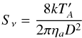
(Rohlfs & Wilson 2004, Eq. (7.18)) where the effective telescope diameter D = 3.28 m and the aperture efficiency ηa ≈ 0.65 (Roelfsema et al. 2012) with a small frequency dependence due to Ruze losses. The factor 2 converts DSB to SSB signal, and  with the forward efficiency ηf = 0.96 (Roelfsema et al. 2012).
As seen from Table 3, the continuum flux densities of our sources generally increase with frequency, as expected for thermal emission from warm dust. The free-free emission of our sources is ≲1 Jy which is negligible (Van der Tak & Menten 2005). For optically thick dust emission at a temperature Td, Sν = Bν(Td) so that in the Rayleigh-Jeans limit, the spectral index α (defined as Sν ∝ να) equals 2, while for optically thin emission, the spectrum steepens to α = 2 + β = 3–4, depending on the far-infrared dust opacity index β, which is 1–2 in most dust models (Ossenkopf & Henning 1994). However, at the high frequencies of our observations and the low average temperatures of our sources (15–40 K: Table 4), deviations from the Rayleigh-Jeans approximation are significant, which reduce these expected spectral indices by ≈1 at Td = 40 K and by ≈2 at Td = 15 K.
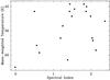 |
Fig. 1 Spectral indices of our sources, calculated from the HIFI continuum levels at 987 and 1669 GHz, versus the mass-weighted temperatures calculated from the models in Sect. 4.1. |
Parameters of continuum models.
The spectral indices of our sources, calculated between 987 and 1670 GHz, are mostly between 1.2 and 2.4 (Fig. 1), which indicates that the emission is close to optically thick. The models in Sect. 4.1 also indicate continuum optical depths around unity at ~1000 GHz. Four sources (NGC 6334I(N), W43 MM1, G327-0.6, and W51e) have lower spectral indices (between 0.0 and 0.5), which for compact sources would suggest low dust temperatures. For extended sources (size ≳15′′), the emission would be resolved at the highest frequencies, which would artificially flatten the spectrum. The model calculations in Sect. 4.1 indicate median source sizes of 17.6, 14.2, and 8.5′′ FWHM at 987, 1113, and 1669 GHz, which is 83%, 75%, and 67% (i.e., most) of the corresponding beam size, suggesting that size effects play a minor role. The importance of dust temperature is also suggested by Fig. 1 which shows that the sources with low spectral indices have low mass-averaged temperatures as calculated from the models in Sect. 4.1. We conclude that our observed variations in the spectral index of the HIFI continuum emission are not due to variations in the source size, but rather to a low dust temperature, both directly and through deviation from the Rayleigh-Jeans law.
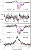 |
Fig. 2 Gaussian decomposition of the observed H2O line profiles (after continuum subtraction) toward IRAS 16272. The envelope component is drawn in red, the broad outflow in green, the narrow outflow in blue, and foreground clouds in purple. |
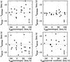 |
Fig. 3 Central velocities of the envelope, narrow outflow, and broad outflow components of the observed H2O lines compared with each other and with the systemic velocity from ground-based data. In the bottom right-hand corner, the typical error bar on the velocities is shown. |
3.2. H2O lines
Figures B.1–B.19 in Appendix B show the observed line profiles. All four lines are detected toward all nineteen sources (except HO toward IRAS 18151), and the line profiles are a mixture of emission and absorption features. Analogous to the case of DR21 (Van der Tak et al. 2010), three physical components appear from these observations (Fig. 2).
First are the protostellar envelopes (also sometimes called dense cores) which usually appear in all four lines in absorption at an LSR velocity known from ground-based millimeter-wave emission line data (Fig. 3, top right); the widths are also similar to the ground-based values. Several sources show two envelope components, due to binarity (e.g., W3 IRS5) or infall/outflow profiles (e.g., W33A, G34.26). The general appearance in absorption indicates a high H2O column density and a low excitation temperature for this component, which is further discussed in Sect. 3.4.
Second are the molecular outflows which usually appear in 1113 and 1669 GHz absorption and 987 GHz emission at velocity offsets of 5–10 km s-1 from the envelope signal and with widths of 10–20 km s-1 FWHM or sometimes more, up to 40 km s-1. Most sources show two outflow components: a broad (ΔV ~ 20 km s-1) and a narrower (ΔV ~ 10 km s-1) feature. In some cases, the width of the narrow outflow feature is similar to that of the corresponding envelope, but the comparison to the ground-based velocity and the presence or absence of HO emission or absorption allows for an unambiguous assignment. The lack of HO signal and the appearance in 987 GHz emission suggest that the outflows have lower H2O column densities and higher excitation temperatures than the envelopes. Section 3.5 discusses the outflow component in detail.
Third are foreground clouds, which appear as narrow (ΔV < 5 km s-1) 1113 and 1669 GHz absorption features at velocities offset by 5−50 km s-1 from the envelope signal. The lack of signal in the 987 GHz and HO lines indicates a low H2O column density and a low excitation temperature for these components, without exception. The number of foreground clouds within the HRS bandwidth ranges from zero toward IRAS 05358 and NGC 7538 to seven toward W51e. Many of these foreground clouds are known from ground-based mm-wave observations of ground-state molecular lines such as CS, HCO+ and HCN (Greaves & Williams 1994; Godard et al. 2010) and from [Hi] 21 cm observations (Fish et al. 2003; Pandian et al. 2008). Other foreground clouds have first been seen with HIFI, such as the V = + 24 km s-1 cloud toward W51e which is seen in HF (Sonnentrucker et al. 2010) but not in our H2O data, and the V = + 13 km s-1 cloud toward AFGL 2591 which is seen in H2O and HF but not in CO (Emprechtinger et al. 2012; Van der Wiel et al. 2013; Choi et al., in prep.). Some foreground clouds are intervening objects on the line of sight, while others represent the “outer envelopes” of large-scale molecular cloud complexes, such as the V = + 65 km s-1 cloud toward W51e (Koo 1997) and two clouds toward NGC 6334 (Van der Wiel et al. 2010). See Sect. 3.6 for further discussion of the foreground clouds.
Our decomposition of the line profiles is similar to the description of H2O line profiles toward low-mass protostars in terms of “narrow”, “medium” and “broad” components (Kristensen et al. 2010), where narrow = envelope, medium = narrow outflow, and broad = broad outflow. Because of the large range in luminosity and mass within our sample, we base the assignment of features to envelope or outflow not only on the line width, but also on the appearance in emission or absorption in the various lines.
3.3. Profile decomposition and flux extraction
We have measured the fluxes ( dV; in emission) and absorbances (∫τdV; in absorption) of the lines by fitting Gaussians to the observed profiles for each line independently. Figure 2 shows IRAS 16272 as an example of the procedure, and the results are presented in Table A.2 for the envelopes, Table A.3 for the outflows, and Table A.4 for the foreground clouds. Our fitting procedure is similar to that by Flagey et al. (2013), where the reader can find further details.
Since some of the emission and absorption features in our data have non-Gaussian shapes, we have verified the results of the Gaussian fitting procedure by a “moment” analysis, which just adds up the flux in all spectrometer channels within a given velocity range. This alternative method extracts the flux of a spectral component independent of its shape, but it cannot handle blending of components, which occurs frequently in our data, unless further assumptions are made. Another disadvantage of the moment method is that the definitions of the velocity ranges are often somewhat arbitrary. After some experimenting, we conclude that fitting Gaussians gives more reliable results than taking moments, if we accept that in some cases, one physical component (usually the outflow) is represented by several (up to three) Gaussians. Another consequence of the non-Gaussian line shape is that the extracted central position and the width of a given component vary somewhat from line to line: up to 2 km s-1 for the envelopes and up to 5 km s-1 for the broad outflow component. The uncertainties on the line positions and widths in Tables A.2, A.3 and A.4 represent this line-to-line variation, whereas the uncertainties on the fluxes and absorbances are dominated by the overall calibration uncertainty (Sect. 2), which is always larger than the formal error of the Gaussian fit caused by the deviation of the observed profile from a Gaussian shape.
For absorption features, Tables A.2–A.4 give the absorbance (=the velocity-integrated optical depth):
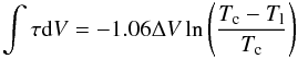 where Tl is the peak depth of the feature, Tc is the SSB continuum temperature, and ΔV is the FWHM line width. For small optical depth, the error on Tl propagates linearly into the absorbance, but if the absorption is almost saturated (Tl → Tc), the error on the absorbance is much larger than that on the measured absorption depth. Cases where the error exceeds the absorbance due to saturation, which occurs mostly for envelope components, are marked with lower limits in Tables A.2–A.4.
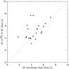 |
Fig. 4 Line widths (FWHM) of the envelope components of the observed H2O lines compared to the widths of the C18O 9–8 line measured with HIFI (San José García et al. 2013). Error bars are smaller than the plotting symbols. |
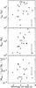 |
Fig. 5 Envelope line width measured from our spectra versus bolometric luminosity (top), envelope mass (middle), and mass/luminosity ratio (bottom). Sources with two envelope features are shown with two data points. In the bottom right-hand corner, the typical uncertainty in the masses, luminosities, and mass/luminosity ratios is shown. |
In the frequent case that absorption and emission features are partially blended, we have estimated the line contribution to the absorption background from the spectra, and added the result to the continuum brightness. This procedure assumes that the absorber is located in front of both the continuum and the line emitting source, which is plausible since in most cases, the absorption depth significantly exceeds the continuum brightness alone.
The model calculations in Sect. 4.1 indicate median source sizes of 17.6, 14.2, and 8.5 arcsec FWHM at 987, 1113, and 1669 GHz, which is 83%, 75%, and 67% of the corresponding beam size. The filling factor would be the square of this fraction which is 68%, 56%, and 45% respectively, so that our absorption line measurements will be affected by covering factor effects if the absorbers are much smaller in size than the beam. In this case, the beam-averaged optical depth would be below the source-averaged value.
3.4. Envelopes
The H2O line spectra of all sources show envelope components, and the velocities and widths of these components in Table A.2 agree well with previous measurements for these sources in other molecules from the ground (Fig. 3). The widths also mostly agree with the widths of the C18O 9–8 line observed with HIFI in a similar beam (Fig. 4); the few cases where ΔV(C18O) > ΔV(H2O) may be influenced by an outflow contribution to the C18O 9–8 line. The measured H2O line widths range over a factor of 4, and show a clear correlation with the envelope masses calculated in Sect. 4.1 (Fig. 5).
The appearance of the envelopes in the four lines differs markedly from source to source, which can be grouped into four types. Seven envelopes appear in absorption in all four lines: G31.41, DR21OH, G327, NGC 6334I(N), IRAS 05358, W43MM1, and one of the G34.26 envelopes. Six envelopes show emission in the 987 GHz line and absorption in the other lines: G10.47, IRAS 18089, W51e, NGC 6334I, IRAS 16272, and one of the W33A envelopes. A further six envelopes appear in H2O 987 GHz and in HO emission, and in H2O 1113 and 1669 GHz absorption: G29.96, NGC 7538, W3 IRS5, G5.89, and the second envelopes of W33A and G34.26. Finally, one source, AFGL 2591, appears in emission in all four lines. One curious case is IRAS 18151, where the non-detection of the HO line leaves ambiguous whether it belongs in the second or third of the above source types; or perhaps it is in a transition from the second to the third type.
One possible origin for the diverse appearance of the envelope features is related to temperature, as appearance in emission (absorption) requires an excitation temperature above (below) the continuum brightness. In this scenario, pure absorption sources would have the most massive and coldest envelopes, sources where the 987 GHz line appears in emission would be somewhat warmer, sources where both H2O 987 GHz and HO appear in emission would be even warmer, and the pure emission source would be the warmest. Alternatively, the appearance of the envelope features in emission or absorption may be a matter of continuum brightness, as detectability in absorption requires a background source whereas emission does not. In particular, the presence of outflow cavities in the HIFI beam would decrease the continuum compared with a beam filled with envelope emission. However, the continuum flux densities in Table 3 do not support this option: the four envelope types above have very similar median continuum brightness levels. Outflow cavities may also affect the H2O line signals, but the net effect may either be emission or absorption, depending on the difference between the H2O excitation temperature and the dust temperature, and on the relative location of dust and water along the line of sight. We conclude that heating effects are more likely than geometric effects to be responsible for the variation in envelope appearance between our sources.
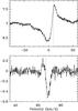 |
Fig. 6 Top: H |
Some sources show two envelope features in some or all H2O line profiles, which in certain cases may be due to the presence of common-envelope binaries at ~1000 AU separation, as suggested for W3 IRS5 (Chavarría et al. 2010). In other cases, the lines have P Cygni or inverse P Cygni profiles, which are due to expansion and infall, respectively (Fig. 6). Such profiles have also been observed in the H2O line spectra of low-mass protostars (Kristensen et al. 2012) and for the low-mass pre-stellar core L1544 (Caselli et al. 2012). Interestingly, the (inverse) P Cygni signature is usually not seen in all lines toward a given source. The sources G10.47 and G34.26 show inverse P Cygni profiles in the H2O 987 GHz and HO lines, suggesting that infall motion only takes place in their inner envelopes. For G34.26, this result is confirmed by SOFIA observations of redshifted NH3 line absorption at 1810 GHz (Wyrowski et al. 2012), and for G10.47 by SMA observations of vibrationally excited HCN (Rolffs et al. 2011). In contrast, G5.89 and DR21OH show P Cygni profiles in the H2O 1113 and 1669 GHz lines and in HO, but not in the H2O 987 GHz line, suggesting that expanding motions only take place in their outer envelopes. In W33A, where only the HO line may show a P Cygni profile, the expanding motion may take place further inside the envelope. For W43 MM1, the low-J lines do not show infall or outflow motions, consistent with the observation by Herpin et al. (2012) that only high-J lines show infall motions in this source, i.e., that infall is confined to the inner envelope. Similar qualitative kinematic variations with radius have been observed in HCN lines toward the Sgr B2 envelope, where the emission peak shifts from blue to red with increasing J, suggesting infall in the outer and expansion in the inner envelope (Rolffs et al. 2010).
3.5. Outflows
The outflows usually show up in the H2O line profiles as two components: a broad (ΔV ~ 10−20 km s-1) emission component visible in all lines, and a narrower (ΔV ~ 5−10 km s-1) absorption component seen in all but the 987 GHz line. Exceptions are AFGL 2591, IRAS 18151 and IRAS 05358, which only show a broad component, and G5.89, which has an exceptionally broad and complex line profile; this source is known to have a very massive and powerful outflow (Acord et al. 1997). For the sources DR21OH, W3 IRS5 and NGC 7538, the widths of the narrower components are so small (2−3 km s-1) that these may be “second envelopes”, as also seen toward W33A and G34.26, and as also advocated by Chavarría et al. (2010) for W3 IRS5. The mm-wave continuum emission from these sources indeed shows multiple spatial components (Woody et al. 1989; Van der Tak et al. 2005), sometimes with mid-infrared counterparts (Megeath et al. 2005; De Wit et al. 2009).
For most of our sources, the broad outflow component appears in emission in all four lines, but there are some exceptions. For AFGL 2591, NGC 6334I, W51e and G34.26, the broad outflow component appears in absorption in the 1113 and 1669 GHz lines, and in emission in the 987 GHz line; for G10.47, this component appears in emission in the 1113 and 987 GHz lines, and in absorption in the 1669 GHz line. Toward W51e, a “very broad” component appears in emission in all four lines between +30 and +90 km s-1. It is unclear in which category G31.41 belongs, since the broad outflow component is only detected in the 987 GHz line, perhaps because in the ground state lines, emission and absorption cancel each other out. The shape of the broad outflow component on the 987 GHz line profile is often non-Gaussian, but the outflow contribution can be modeled with two Gaussians of about the same height and width. In this case the velocity in Table A.3 is the mean of the values for the two Gaussians, while the width and the flux are the sums.
The narrow outflow component usually appears in absorption in the H2O 1113 and 1669 GHz lines and the HO line, and is not seen in the H2O 987 GHz line, but again, exceptions occur. For W3 IRS5, G327 and G31.41, the narrow outflow component appears in 1113 and 1669 GHz absorption and in 987 GHz emission; for IRAS 18089 and G34.26, this component appears in 1113 and 1669 GHz absorption and in HO emission, while for G10.47, it appears in emission in all four lines. Unlike the envelopes, the outflow absorptions are usually not saturated, with G327 as only exception.
We have used the measured velocities of the outflow components to test if our sources have a preferred orientation in the sky. In particular, for a face-on geometry, the outflow would be directed toward us, and thus appear blueshifted relative to the envelope component if seen in absorption. The narrow outflow component is the one that is usually seen in absorption, and Fig. 3 shows that this component is indeed usually blueshifted relative to the envelope. The exceptions are IRAS 16272, DR21(OH), G29.96, and W51e, and Fig. 2 illustrates the case of IRAS 16272, especially for the 1669 GHz line. The widths of these redshifted absorption features are too large to be due to infall motions, and we suggest that these sources have binaries or other deviations from centrosymmetric geometry that allow their receding outflow lobes to show in absorption. In addition, Fig. 7 shows that there are no clear trends between the widths of the envelope and outflow components.
Figure 8 compares the widths of the broad outflow components to the widths observed in CO 3–2 with the JCMT (San José García et al. 2013). While sources with broader H2O outflows also seem to have broader CO outflows, the width for any given source is larger in CO than in H2O by about 10 km s-1. This result is contrary to the case of low-mass protostars, where the H2O line widths exceed those of CO (Kristensen et al. 2012). For our sources, the H2O may be confined to denser gas where velocities are lower. Alternatively, the difference is excitation: our H2O values are averages over ground-state and excited-state lines, while the outflow line widths increase with J or Eup. Indeed, the widths of the excited-state H2O lines are very close to those measured in CO, as also found by Chavarría et al. (2010) and Herpin et al. (2012).
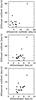 |
Fig. 7 Line widths (FWHM) of the envelope, narrow outflow, and broad outflow components of the observed H2O lines compared with each other. Error bars are smaller than the plotting symbols. |
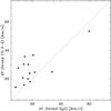 |
Fig. 8 Line widths (FWHM) of the broad outflow components of the observed H2O lines compared to the widths of the CO 3–2 lines measured with the JCMT (San José García et al. 2013). Error bars are smaller than the plotting symbols. |
3.6. Foreground clouds
The foreground clouds appear as narrow (ΔV = 1−4 km s-1) absorption features in the 1113 and 1669 GHz line spectra of our sources. While one cloud also shows HO absorption, the general lack of signal in the H2O 987 GHz and HO lines indicates a low column density and a low volume density for these clouds. The last two columns of Table A.4 list estimates of the H2O column densities and ortho-para ratios of the foreground clouds. These values were obtained from the velocity-integrated optical depths in the table by assuming that in these clouds, all H2O molecules are in their ortho and para ground states, i.e., that excitation is negligible. As discussed by Emprechtinger et al. (2013), this assumption generally holds for column density estimates from the 1113 and 1669 GHz lines, but fails for the H2O 557 GHz line.
The H2O column densities of the foreground clouds are found to lie mostly in the range 1 × 10¹²–1 × 1013 cm-2, with a few outliers at the upper and lower end. These values are comparable to earlier estimates (Van der Tak et al. 2010; Lis et al. 2010) and indicate that the H2O abundance in these clouds is limited by photodissociation. The derived ortho/para ratios for H2O lie mostly in the range between 3 and 6, again with a few outliers to higher and lower values. Our derived o/p ratios are very similar to the values by Lis et al. (2010) and Herpin et al. (2012). Comparison to the detailed multi-line study by Flagey et al. (2013) for the 5 overlapping sources suggests that our estimated column densities and o/p ratios for individual clouds have uncertainties of a factor of ~2, which is an upper limit since not exactly the same positions were observed.
The ortho-para ratio of H2O is expected to rise from ≈1.0 at low temperatures (≈15 K) to ≈3 at high temperatures (≳50 K) as shown by Mumma et al. (1987). Even though the values derived here are probably uncertain to a factor of ~2, our results are inconsistent with the low-temperature limit. If the H2O molecules were formed on cold (10 K) grain surfaces, their spin temperature does not reflect these conditions, and may instead be set by the grain temperature shortly before the H2O ice mantle evaporated (at T ≈100 K). Alternatively, the H2O molecules may have formed in the warm (Tkin ≈ 50 K) gas phase by ion-molecule reactions, or the o/p ratio of the evaporated H2O may have equilibrated with that of H2 in the warm gas phase in reactions with H .
.
4. Analysis and discussion
4.1. Mass estimation
Estimates of the envelope masses exist in the literature for many of our sources. However, these mass estimations were performed by different authors, using different techniques and based on data from different telescopes. In order to have a homogeneous mass determination over our sample, we derive the envelope mass by comparing models of the continuum spectral energy distribution (SED) with the available observations for each source.
We use a modified version of the 3D continuum radiative transfer code HOCHUNK3D (Whitney et al. 2013; Robitaille 2011, hereafter WR) to find the envelope temperature profile and derive a model SED for each source. Our modified version of the code uses dust opacities from Ossenkopf & Henning (1994), model 5 with thin ice mantles and a gas density of 106 cm-3, suitable for high-mass protostars (Van der Tak et al. 1999), and allows to vary the radial density power-law exponent p. The WR code allows for a detailed description of the protostellar environment in terms of a star, a disk, a cavity and an envelope. To decrease the number of free parameters, we use a simple spherically symmetric model with no cavity and no disk. This simplification has its main effect in the near to mid-infrared region of the spectrum, while the sub-millimeter and millimeter-wave regions, where the dust is mainly emitting, will stay almost unchanged.
The envelope size and density exponent p are derived from archival sub-millimeter images from the JCMT/SCUBA4 and APEX/LABOCA (Siringo et al. 2009) instruments. For the envelope size, we choose the radius of the contour at the 3σ noise level, while for the density exponent, we use the WR code to create synthetic sub-millimeter maps for various p-values. We determine the best-fit density exponent by minimizing the difference between the observed and synthetic brightness profiles (see Fig. 9). The synthetic maps are created using the corresponding instrumental pass-band and convolved with the instrumental beam profile including the error-beam.
With the outer radius and the density profile fixed, the only remaining parameters are the envelope mass and the bolometric luminosity. The observed fluxes from the literature correspond to the peak emission at the source position. In most cases, the beam size of the observed fluxes is smaller than the source size. To correct for the missing flux, we normalize the observed fluxes by the ratio between the flux from the whole model and the flux from a region as big as the beam size. As an example, Fig. 10 shows the observed and derived SED for the source IRAS 16272 as well as the temperature profile. Table 4 lists the adopted and the derived physical parameters for each source, and Appendix C presents the results in graphical form.
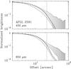 |
Fig. 9 Submillimeter brightness profiles of AFGL 2591 measured with JCMT/SCUBA (error bars), and synthetic brightness profiles derived from WR models and convolved by the SCUBA beams for p = 1.0 (solid line) and p = 1.5 (dashed line). The vertical dotted line indicates the adopted source radius. For this source, we choose a density profile of p = 1.0. |
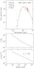 |
Fig. 10 Top: model (continuous line) and observed SED fluxes (error bars) for IRAS 16272. The SED points are normalized by the source size for λ > 100 microns, as shown by the “X” symbols. Continuum flux densities from our HIFI data are labeled in red. Bottom: temperature and density profiles for IRAS 16272. |
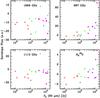 |
Fig. 11 Envelope line flux versus 60 μm flux density. Uncertainties are ≈10% for HIFI data and ≈20% for IRAS data. Open red and filled green squares are mid-IR-quiet and -bright protostellar objects, filled blue triangles are hot molecular cores, and filled purple circles are ultracompact Hii regions. |
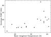 |
Fig. 12 Envelope H2O 987 GHz line flux versus mass-weighted temperature in our envelope models. |
4.2. Correlations with luminosity and mass
To understand the origin of the observed H2O lines, we now investigate if the measured line fluxes show trends with the luminosity of the source Lbol (Table 1) and the mass of the envelope Menv (Table 4). In addition, we have searched for trends with distance but did not find any. For the luminosity, we use the results of the model fit in Sect. 4.1 so that the source flux at all wavelengths refers to the same area on the sky. Figures D.1−D.3 in Appendix D show scatter plots of the line fluxes of the envelope and the narrow and broad outflow components versus Lbol and Menv. In these figures, absorption is plotted as negative emission, and “double envelope” features are plotted as two data points. We identify possible trends by visual inspection of these plots, and test these (if applicable) by computing the correlation coefficient r and the probability of false correlation P, which depends on r and the number of data points N (see Appendix of Marseille et al. 2010a).
For the envelope component, the visual inspection reveals two trends. First, the 987 GHz line flux increases with Lbol, but only if the line appears in emission. This trend is not a correlation, but more a “threshold effect”: strong 987 GHz line emission is only seen at high luminosities (Lbol ≳105 L⊙). Second, the HO line flux decreases with increasing Menv, but again not as a correlation but in the sense that the line is seen in emission at low Menv and absorption for high Menv. Such behavior is expected if the line optical depth, and thus the H2O column density, increases with envelope mass. An optical depth of ~unity for the HO line is confirmed by detections of HO line emission in several of our sources (Herpin et al. 2012; Choi et al., in prep.). Apparently the average H2O abundance is rather constant across all envelopes in our source sample. The studies mentioned in Sect. 1 indicate outer envelope abundances of ~10-9–10-8.
The increase of the 987 GHz line flux with Lbol is probably due to a higher temperature of the inner envelopes of sources with a higher luminosity. This idea is confirmed by the trend between 987 GHz line flux with far-infrared continuum flux density (Fig. 11). Such a trend is seen both at 60 and at 100 μm, and like the trend with Lbol, is more a threshold effect than a correlation. The large beam size of IRAS may influence these trends quantitatively, but probably has no strong qualitative effect because our sources were selected to be relatively isolated (Sect. 1). Far-infrared pumping could influence the results for individual H2O lines, but is unlikely to dominate here, because the effect is seen in several lines.
Further evidence that the H2O 987 GHz line flux is due to envelope heating is presented in Fig. 12, which is a plot of the flux in this line versus the mass-weighted temperature from the envelope models in Sect. 4.1. While a 1:1 correlation cannot be claimed, the points show a clear trend toward higher line fluxes at higher average temperatures.
Figures D.2 and D.3 show a similar analysis for the narrow and broad outflow components in the H2O line profiles of our sources. The most significant trend is that the HO line flux of the broad outflow component decreases with increasing Lbol (r = − 0.683, P = 3%), but only in the 11 cases where this component is detected in HO. Second, the 987 GHz line flux of the broad outflow component appears to increase with increasing Menv, but with r = 0.174 and P = 14%, this trend is less significant than the first one. The line fluxes of the narrow outflow component do not show any clear trends with Lbol or Menv.
The lack of evolutionary trends in the H2O line fluxes of our sources is in contrast with the study of López-Sepulcre et al. (2011), who observed the SiO J = 2–1 and 3–2 lines toward 57 high-mass star-forming regions, and found that the SiO line luminosity drops with evolutionary stage as measured by increasing values of Lbol/Menv. This drop suggests a decline of the jet activity with the evolutionary state of the source, as also observed for low-mass sources (Bontemps et al. 1996), although excitation effects also may play a role.
One reason for this difference may be that even the H2O line signals from the outflows may be somewhat optically thick, so that saturation masks any evolutionary trends. Therefore, we consider next trends of the line width with Lbol and Menv. The line width is less sensitive to the optical depth than the line intensity, and has the additional advantage that the appearance of the line in emission or absorption does not influence its measurement. Section 3.4 already shows the trend of the envelope ΔV with Menv, which with r = 0.407 and P = 4% for N = 22 is likely real.
Figures D.4 and D.5 show scatter plots of the widths of the narrow and broad outflow components versus Lbol and Menv. The only significant trend that appears is that ΔV of the narrow outflow component increases with Menv. A relation of this component with the envelope has been found before for low-mass protostars (Kristensen et al. 2012), and suggests that the narrow outflow component is due to outflow-envelope interactions.
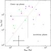 |
Fig. 13 Bolometric luminosity versus envelope mass for our sources, where the dotted line divides the two phases of high-mass protostellar evolution suggested by Molinari et al. (2008) and the dashed arrow is a typical evolutionary track. The typical uncertainty of a factor of 2 in both luminosity and mass is indicated at the bottom. Symbols are as in Fig. 11. |
4.3. Evolutionary trends
We now discuss several proposed evolutionary indicators for high-mass star formation and test them on our source sample. We will use the ratio of Lbol over Menv as primary evolutionary indicator, because of previous success (Van der Tak et al. 2000; Motte et al. 2007; López-Sepulcre et al. 2010), because it is a continuous variable, and because it has a physical basis (declining accretion activity and envelope dispersal). In particular, Molinari et al. (2008) have proposed an evolutionary sequence for high-mass protostars in terms of two parameters: the envelope mass and the bolometric luminosity. They suggest a two-step evolutionary sequence: protostars first accrete mass from their envelopes, and later disperse their envelopes by winds and/or radiation. In the diagram in Fig. 13, their calculated evolutionary tracks start at the bottom, rise upward until they reach the dotted line, and then proceed horizontally to the left. The positions of our sources in this diagram suggest that the subsample of mid-IR-quiet protostellar objects is the youngest, and that the other subsamples contain more evolved sources. The same effect is seen in Figs. D.1–D.3, where the mid-IR-quiet protostellar objects occupy the left (low-Lbol) sides of the diagrams. On the other hand, the presence of a hot molecular core and/or an ultracompact Hii region is unrelated to mid-infrared brightness and Lbol/Menv ratio, at least for our sample. The occurrence of these phenomena may depend more on absolute luminosity than on evolutionary stage.
To test the use of H2O line profiles as evolutionary indicators, we use the appearance of the envelope component in the H2O ground-state line profiles, as introduced in Sect. 3.4. In Type 1 sources, all lines appear in absorption; Type 2 sources show emission in the 987 GHz line and absorption in the others; in Type 3 sources, both the 987 GHz and the HO lines appear in emission; and Type 4 sources show all lines in emission. While the Type 1 sources all seem to be in early evolutionary stages as probed by a low Lbol/Menv ratio, the other source types are all mixed. Thus, an H2O line profile with pure absorption appears to be a sign of an early evolutionary stage, whereas emission is a sign of a more evolved stage.
The appearance of the broad and narrow outflow components in the H2O ground-state line profiles differs between our sources, and for each component, four types may be defined as for the envelopes (Sect. 3.5). While these emission/absorption types may be useful to trace protostellar evolution, our data do not allow to tesdt this hypothesis, since most of our sources belong to just one of these types, with the broad outflow appearing in absorption and the narrow outflow in emission. This issue may be revisited after HIFI data become available for a larger sample of sources outside the WISH program.
Besides the shape of the line profile, the fluxes and widths of the H2O line may also be evolutionary indicators. The bottom panels of Figs. D.1–D.3 show scatter plots of our observed line fluxes in the envelope and outflow components versus the ratio Menv/Lbol which as discussed above is sometimes used as evolutionary indicator for high-mass protostars. No trends appear, and the same is true for the plots of the line width versus Menv/Lbol (Figs. 5, D.4 and D.5).
5. Summary and conclusions
This paper presents spectroscopic observations of low-J H2O transitions observed toward 19 regions of high-mass star formation. The line profiles show contributions from protostellar envelopes, bipolar outflows, and foreground clouds. These contributions, both in emission and in absorption, are disentangled by fitting multiple Gaussians to the line profiles.
Our observations show that the ground state lines of H2O are powerful tracers of the various physical and kinematic components of the high-mass protostellar environment, as well as of foreground clouds. The envelope components of the ground state lines of H2O at 1113 and 1669 GHz do not show significant trends with bolometric luminosity, envelope mass, or far-infrared flux density or color, indicating that these lines trace the outer parts of the envelopes where the effects of star formation are hardly noticeable. On the other hand, broad wings due to outflows are clearly seen in these lines, which are a clear effect of star formation. The competing effects of line emission and absorption in the ground-state lines lead to low integrated line fluxes, which may explain the difficulty in detecting these lines in distant galaxies.
Unlike the ground-state lines, the flux in the excited-state 987 GHz line increases systematically with luminosity and with the far-infrared flux density, both at 60 and at 100 μm. This line therefore appears to be a good tracer of the average temperature of the source. Indeed, this line and other excited-state lines have proven to be more easily detected at high redshift (Omont et al. 2011; Van der Werf et al. 2011).
Furthermore, the HO ground-state line turns from emission into absorption with increasing envelope mass. This trend indicates that the H2O abundances in protostellar envelopes do not change much with time.
The appearance of the H2O line profiles in our sample changes with evolutionary state, in the sense that the youngest sources (as probed by mid-infrared brightness and Lbol/Menv ratio) show pure absorption profiles for all lines, while for more evolved sources, one or more of our studied lines appears in emission. This effect is visible for the envelope component but not for the outflows. In addition, the presence of infall or expansion, as probed by (inverse) P Cygni profiles, does not appear related to evolutionary stage.
In the future, our team will make detailed estimates of the H2O abundances in these sources as a function of radius, based on HIFI observations of ≈20 lines of H2O, HO and HO. The Herschel/PACS instrument will be used to study higher-excitation H2O lines and to improve estimates of the bolometric temperatures of our sources, which may act as evolutionary indicator. Maps of selected lines with HIFI and PACS will clarify the spatial distribution of H2O, both on the scale of protostellar envelopes and outflows as on larger (protostellar cluster) scales. On smaller scales, ALMA will provide images of high-excitation H2O and HO lines and thus zoom into the close vicinity of the central protostars.
Online material
Appendix A: Observation log and line flux tables
List of observations.
Central velocities, FWHM widths, and integrated line fluxes measured for the protostellar envelopes.
Appendix B: Observed line profiles
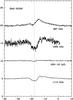 |
Fig. B.1 Spectra of the H2O 111 − 000 (bottom), H |
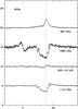 |
Fig. B.8 As Fig. B.1, toward W33A. The emission/absorption feature near 0 km s-1 in the 1669 GHz spectrum is the H2O 1661 GHz line from the other sideband. |
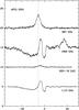 |
Fig. B.10 As Fig. B.1, toward AFGL 2591. The emission feature near +18 km s-1 in the 1669 GHz spectrum is the H2O 1661 GHz line from the other sideband. |
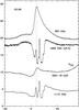 |
Fig. B.15 As Fig. B.1, toward G5.89. The emission feature near +90 km s-1 in the H |
Appendix C: Continuum models
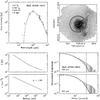 |
Fig. C.1 Continuum model for IRAS 05358. Top left: spectral energy distribution. Top right: submillimeter image with 3σ contour marked in white and useable map sectors marked in black. Bottom left: temperature and density structure as a function of radius. Bottom right: submillimeter emission profiles. The numbers in the top left panel are the modeled envelope mass, the modeled luminosity, the adopted envelope size and the adopted distance. |
Appendix D: Correlation analysis
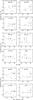 |
Fig. D.1 Observed line fluxes (positive: emission) or absorbances (negative: absorption) versus bolometric luminosity L of the source (top), versus envelope mass M (middle), and versus the ratio L/M (bottom). Open squares: mid-IR-quiet HMPOs; filled squares: mid-IR-bright HMPOs; triangles: hot molecular cores; circles: ultracompact Hii regions. Uncertainties in line fluxes are ≈10%, while the typical uncertainty of masses, luminosities and L/M ratios is a factor of 2. |
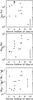 |
Fig. D.4 Line width of the narrow outflow component versus bolometric luminosity L of the source (top), versus envelope mass M (middle), and versus the ratio L/M (bottom). The error bar denotes the typical uncertainty in mass, luminosity, and L/M ratio; the uncertainty in line width is smaller than the symbol size. |
Acknowledgments
This paper is dedicated to the memory of Annemieke Gloudemans-Boonman, a pioneer of H2O observations with ISO, who passed away on 11 October 2010 at the age of 35. We thank Umut Yildiz for maintaining the WISH data archive (the “live show”), Agata Karska for providing PACS continuum fluxes of our sources, and the referee for carefully reading our manuscript and writing a constructive report. This work has used the spectroscopic databases of JPL (Pickett et al. 1998) and CDMS (Müller et al. 2001), and the facilities of the Canadian Astronomy Data Centre operated by the the National Research Council of Canada with the support of the Canadian Space Agency. L.C. thanks the Spanish MINECO for funding support from grant AYA2009-07304. HIFI has been designed and built by a consortium of institutes and university departments from across Europe, Canada and the US under the leadership of SRON Netherlands Institute for Space Research, Groningen, The Netherlands with major contributions from Germany, France and the US. Consortium members are: Canada: CSA, U.Waterloo; France: CESR, LAB, LERMA, IRAM; Germany: KOSMA, MPIfR, MPS; Ireland, NUI Maynooth; Italy: ASI, IFSI-INAF, Arcetri-INAF; Netherlands: SRON, TUD; Poland: CAMK, CBK; Spain: Observatorio Astronómico Nacional (IGN), Centro de Astrobiología (CSIC-INTA); Sweden: Chalmers University of Technology – MC2, RSS & GARD, Onsala Space Observatory, Swedish National Space Board, Stockholm University – Stockholm Observatory; Switzerland: ETH Zürich, FHNW; USA: Caltech, JPL, NHSC.
References
- Acord, J. M., Walmsley, C. M., & Churchwell, E. 1997, ApJ, 475, 693 [NASA ADS] [CrossRef] [Google Scholar]
- Beuther, H., Schilke, P., Gueth, F., et al. 2002, A&A, 387, 931 [NASA ADS] [CrossRef] [EDP Sciences] [Google Scholar]
- Bjerkeli, P., Liseau, R., Olberg, M., et al. 2009, A&A, 507, 1455 [NASA ADS] [CrossRef] [EDP Sciences] [Google Scholar]
- Bontemps, S., Andre, P., Terebey, S., & Cabrit, S. 1996, A&A, 311, 858 [NASA ADS] [Google Scholar]
- Caselli, P., Keto, E., Bergin, E. A., et al. 2012, ApJ, 759, L37 [Google Scholar]
- Cernicharo, J., Thum, C., Hein, H., et al. 1990, A&A, 231, L15 [NASA ADS] [Google Scholar]
- Cesaroni, R., Hofner, P., Walmsley, C. M., & Churchwell, E. 1998, A&A, 331, 709 [NASA ADS] [Google Scholar]
- Chavarría, L., Herpin, F., Jacq, T., et al. 2010, A&A, 521, L37 [NASA ADS] [CrossRef] [EDP Sciences] [Google Scholar]
- Cheung, A. C., Rank, D. M., Townes, C. H., Thornton, D. D., & Welch, W. J. 1969, Nature, 221, 626 [NASA ADS] [CrossRef] [Google Scholar]
- Churchwell, E., Walmsley, C. M., & Cesaroni, R. 1990, A&AS, 83, 119 [NASA ADS] [Google Scholar]
- De Graauw, T., Helmich, F. P., Phillips, T. G., et al. 2010, A&A, 518, L6 [NASA ADS] [CrossRef] [EDP Sciences] [Google Scholar]
- De Wit, W. J., Hoare, M. G., Fujiyoshi, T., et al. 2009, A&A, 494, 157 [NASA ADS] [CrossRef] [EDP Sciences] [Google Scholar]
- Emprechtinger, M., Lis, D. C., Bell, T., et al. 2010, A&A, 521, L28 [NASA ADS] [CrossRef] [EDP Sciences] [Google Scholar]
- Emprechtinger, M., Monje, R. R., van der Tak, F. F. S., et al. 2012, ApJ, 756, 136 [NASA ADS] [CrossRef] [Google Scholar]
- Emprechtinger, M., Lis, D. C., Rolffs, R., et al. 2013, ApJ, 765, 61 [NASA ADS] [CrossRef] [Google Scholar]
- Faúndez, S., Bronfman, L., Garay, G., et al. 2004, A&A, 426, 97 [NASA ADS] [CrossRef] [EDP Sciences] [Google Scholar]
- Fish, V. L., Reid, M. J., Wilner, D. J., & Churchwell, E. 2003, ApJ, 587, 701 [NASA ADS] [CrossRef] [Google Scholar]
- Flagey, N., Goldsmith, P. F., Lis, D. C., et al. 2013, ApJ, 762, 11 [NASA ADS] [CrossRef] [Google Scholar]
- Garay, G., Brooks, K. J., Mardones, D., Norris, R. P., & Burton, M. G. 2002, ApJ, 579, 678 [NASA ADS] [CrossRef] [MathSciNet] [Google Scholar]
- Godard, B., Falgarone, E., Gerin, M., Hily-Blant, P., & de Luca, M. 2010, A&A, 520, A20 [NASA ADS] [CrossRef] [EDP Sciences] [Google Scholar]
- Greaves, J. S., & Williams, P. G. 1994, A&A, 290, 259 [NASA ADS] [Google Scholar]
- Hachisuka, K., Brunthaler, A., Menten, K. M., et al. 2006, ApJ, 645, 337 [NASA ADS] [CrossRef] [Google Scholar]
- Hatchell, J., & van der Tak, F. F. S. 2003, A&A, 409, 589 [NASA ADS] [CrossRef] [EDP Sciences] [Google Scholar]
- Herpin, F., Chavarría, L., van der Tak, F., et al. 2012, A&A, 542, A76 [NASA ADS] [CrossRef] [EDP Sciences] [Google Scholar]
- Hunter, T. R., Churchwell, E., Watson, C., et al. 2000, AJ, 119, 2711 [NASA ADS] [CrossRef] [Google Scholar]
- Immer, K., Reid, M. J., Menten, K. M., Brunthaler, A., & Dame, T. M. 2013, A&A, 553, A117 [NASA ADS] [CrossRef] [EDP Sciences] [Google Scholar]
- Jakob, H., Kramer, C., Simon, R., et al. 2007, A&A, 461, 999 [NASA ADS] [CrossRef] [EDP Sciences] [Google Scholar]
- Jørgensen, J. K., & van Dishoeck, E. F. 2010, ApJ, 710, L72 [NASA ADS] [CrossRef] [Google Scholar]
- Koo, B.-C. 1997, ApJS, 108, 489 [NASA ADS] [CrossRef] [Google Scholar]
- Kristensen, L. E., Visser, R., van Dishoeck, E. F., et al. 2010, A&A, 521, L30 [NASA ADS] [CrossRef] [EDP Sciences] [Google Scholar]
- Kristensen, L. E., van Dishoeck, E. F., Bergin, E. A., et al. 2012, A&A, 542, A8 [NASA ADS] [CrossRef] [EDP Sciences] [Google Scholar]
- Kuchar, T. A., & Bania, T. M. 1994, ApJ, 436, 117 [NASA ADS] [CrossRef] [Google Scholar]
- Ladd, E. F., Deane, J. R., Sanders, D. B., & Wynn-Williams, C. G. 1993, ApJ, 419, 186 [NASA ADS] [CrossRef] [Google Scholar]
- Lester, D. F., Dinerstein, H. L., Werner, M. W., et al. 1985, ApJ, 296, 565 [NASA ADS] [CrossRef] [Google Scholar]
- Lis, D. C., Phillips, T. G., Goldsmith, P. F., et al. 2010, A&A, 521, L26 [NASA ADS] [CrossRef] [EDP Sciences] [Google Scholar]
- López-Sepulcre, A., Cesaroni, R., & Walmsley, C. M. 2010, A&A, 517, A66 [NASA ADS] [CrossRef] [EDP Sciences] [Google Scholar]
- López-Sepulcre, A., Walmsley, C. M., Cesaroni, R., et al. 2011, A&A, 526, L2 [NASA ADS] [CrossRef] [EDP Sciences] [Google Scholar]
- Marseille, M. G., van der Tak, F. F. S., Herpin, F., & Jacq, T. 2010a, A&A, 522, A40 [NASA ADS] [CrossRef] [EDP Sciences] [Google Scholar]
- Marseille, M. G., van der Tak, F. F. S., Herpin, F., et al. 2010b, A&A, 521, L32 [Google Scholar]
- Megeath, S. T., Wilson, T. L., & Corbin, M. R. 2005, ApJ, 622, L141 [NASA ADS] [CrossRef] [Google Scholar]
- Melnick, G. J., & Bergin, E. A. 2005, Adv. Space Res., 36, 1027 [NASA ADS] [CrossRef] [Google Scholar]
- Menten, K. M., Melnick, G. J., Phillips, T. G., & Neufeld, D. A. 1990, ApJ, 363, L27 [NASA ADS] [CrossRef] [Google Scholar]
- Minier, V., André, P., Bergman, P., et al. 2009, A&A, 501, L1 [NASA ADS] [CrossRef] [EDP Sciences] [Google Scholar]
- Molinari, S., Brand, J., Cesaroni, R., & Palla, F. 1996, A&A, 308, 573 [NASA ADS] [Google Scholar]
- Molinari, S., Pezzuto, S., Cesaroni, R., et al. 2008, A&A, 481, 345 [NASA ADS] [CrossRef] [EDP Sciences] [Google Scholar]
- Moscadelli, L., Reid, M. J., Menten, K. M., et al. 2009, ApJ, 693, 406 [NASA ADS] [CrossRef] [Google Scholar]
- Motogi, K., Sorai, K., Habe, A., et al. 2011, PASJ, 63, 31 [NASA ADS] [Google Scholar]
- Motte, F., Bontemps, S., Schilke, P., et al. 2007, A&A, 476, 1243 [NASA ADS] [CrossRef] [EDP Sciences] [Google Scholar]
- Mueller, K. E., Shirley, Y. L., Evans, II, N. J., & Jacobson, H. R. 2002, ApJS, 143, 469 [NASA ADS] [CrossRef] [Google Scholar]
- Müller, H. S. P., Thorwirth, S., Roth, D. A., & Winnewisser, G. 2001, A&A, 370, L49 [NASA ADS] [CrossRef] [EDP Sciences] [Google Scholar]
- Mumma, M. J., Weaver, H. A., & Larson, H. P. 1987, A&A, 187, 419 [NASA ADS] [Google Scholar]
- Neckel, T. 1978, A&A, 69, 51 [NASA ADS] [Google Scholar]
- Nguyen Luong, Q., Motte, F., Schuller, F., et al. 2011, A&A, 529, A41 [NASA ADS] [CrossRef] [EDP Sciences] [Google Scholar]
- Omont, A., Neri, R., Cox, P., et al. 2011, A&A, 530, L3 [NASA ADS] [CrossRef] [EDP Sciences] [Google Scholar]
- Ossenkopf, V., & Henning, T. 1994, A&A, 291, 943 [NASA ADS] [Google Scholar]
- Pandian, J. D., Momjian, E., & Goldsmith, P. F. 2008, A&A, 486, 191 [NASA ADS] [CrossRef] [EDP Sciences] [Google Scholar]
- Pickett, H. M., Poynter, R. L., Cohen, E. A., et al. 1998, J. Quant. Spec. Radiat. Transf., 60, 883 [Google Scholar]
- Pilbratt, G. L., Riedinger, J. R., Passvogel, T., et al. 2010, A&A, 518, L1 [CrossRef] [EDP Sciences] [Google Scholar]
- Pratap, P., Megeath, S. T., & Bergin, E. A. 1999, ApJ, 517, 799 [NASA ADS] [CrossRef] [Google Scholar]
- Reid, M. J., Menten, K. M., Zheng, X. W., et al. 2009, ApJ, 700, 137 [NASA ADS] [CrossRef] [Google Scholar]
- Robitaille, T. P. 2011, A&A, 536, A79 [NASA ADS] [CrossRef] [EDP Sciences] [Google Scholar]
- Roelfsema, P. R., Helmich, F. P., Teyssier, D., et al. 2012, A&A, 537, A17 [NASA ADS] [CrossRef] [EDP Sciences] [Google Scholar]
- Rohlfs, K., & Wilson, T. L. 2004, Tools of radio astronomy (Berlin: Springer) [Google Scholar]
- Rolffs, R., Schilke, P., Comito, C., et al. 2010, A&A, 521, L46 [NASA ADS] [CrossRef] [EDP Sciences] [Google Scholar]
- Rolffs, R., Schilke, P., Zhang, Q., & Zapata, L. 2011, A&A, 536, A33 [NASA ADS] [CrossRef] [EDP Sciences] [Google Scholar]
- Rygl, K. L. J., Brunthaler, A., Sanna, A., et al. 2012, A&A, 539, A79 [NASA ADS] [CrossRef] [EDP Sciences] [Google Scholar]
- San José García, I., Mottram, J. C., Kristensen, L., et al. 2013, A&A, 553, A125 [NASA ADS] [CrossRef] [EDP Sciences] [Google Scholar]
- Sandell, G. 2000, A&A, 358, 242 [NASA ADS] [Google Scholar]
- Sandell, G., & Sievers, A. 2004, ApJ, 600, 269 [NASA ADS] [CrossRef] [Google Scholar]
- Sanna, A., Reid, M. J., Carrasco-González, C., et al. 2012a, ApJ, 745, 191 [NASA ADS] [CrossRef] [Google Scholar]
- Sanna, A., Reid, M. J., Dame, T. M., et al. 2012b, ApJ, 745, 82 [NASA ADS] [CrossRef] [Google Scholar]
- Siringo, G., Kreysa, E., Kovács, A., et al. 2009, A&A, 497, 945 [NASA ADS] [CrossRef] [EDP Sciences] [Google Scholar]
- Sonnentrucker, P., Neufeld, D. A., Phillips, T. G., et al. 2010, A&A, 521, L12 [NASA ADS] [CrossRef] [EDP Sciences] [Google Scholar]
- Sridharan, T. K., Beuther, H., Schilke, P., Menten, K. M., & Wyrowski, F. 2002, ApJ, 566, 931 [NASA ADS] [CrossRef] [Google Scholar]
- Trinidad, M. A., Curiel, S., Cantó, J., et al. 2003, ApJ, 589, 386 [NASA ADS] [CrossRef] [Google Scholar]
- Urquhart, J. S., Hoare, M. G., Lumsden, S. L., et al. 2012, MNRAS, 420, 1656 [NASA ADS] [CrossRef] [Google Scholar]
- Van der Tak, F. F. S., & Menten, K. M. 2005, A&A, 437, 947 [NASA ADS] [CrossRef] [EDP Sciences] [Google Scholar]
- Van der Tak, F. F. S., van Dishoeck, E. F., Evans, II, N. J., Bakker, E. J., & Blake, G. A. 1999, ApJ, 522, 991 [NASA ADS] [CrossRef] [Google Scholar]
- Van der Tak, F. F. S., van Dishoeck, E. F., Evans, II, N. J., & Blake, G. A. 2000, ApJ, 537, 283 [NASA ADS] [CrossRef] [Google Scholar]
- Van der Tak, F. F. S., Tuthill, P. G., & Danchi, W. C. 2005, A&A, 431, 993 [NASA ADS] [CrossRef] [EDP Sciences] [Google Scholar]
- Van der Tak, F. F. S., Walmsley, C. M., Herpin, F., & Ceccarelli, C. 2006, A&A, 447, 1011 [NASA ADS] [CrossRef] [EDP Sciences] [Google Scholar]
- Van der Tak, F. F. S., Marseille, M. G., Herpin, F., et al. 2010, A&A, 518, L107 [Google Scholar]
- Van der Werf, P. P., Berciano Alba, A., Spaans, M., et al. 2011, ApJ, 741, L38 [NASA ADS] [CrossRef] [Google Scholar]
- Van der Wiel, M. H. D., van der Tak, F. F. S., Lis, D. C., et al. 2010, A&A, 521, L43 [Google Scholar]
- Van der Wiel, M. H. D., Pagani, L., van der Tak, F. F. S., Kazmierczak, M., & Ceccarelli, C. 2013, A&A, 553, A11 [NASA ADS] [CrossRef] [EDP Sciences] [Google Scholar]
- Van Dishoeck, E. F., & Helmich, F. P. 1996, A&A, 315, L177 [NASA ADS] [Google Scholar]
- Van Dishoeck, E. F., Kristensen, L. E., Benz, A. O., et al. 2011, PASP, 123, 138 [NASA ADS] [CrossRef] [Google Scholar]
- Wang, K.-S., van der Tak, F. F. S., & Hogerheijde, M. R. 2012, A&A, 543, A22 [NASA ADS] [CrossRef] [EDP Sciences] [Google Scholar]
- Watson, D. M., Bohac, C. J., Hull, C., et al. 2007, Nature, 448, 1026 [NASA ADS] [CrossRef] [PubMed] [Google Scholar]
- Whitney, B., Robitaille, T., Bjorkman, J., et al. 2013, ApJS, submitted [Google Scholar]
- Wood, D. O. S., & Churchwell, E. 1989, ApJS, 69, 831 [NASA ADS] [CrossRef] [Google Scholar]
- Woody, D. P., Scott, S. L., Scoville, N. Z., et al. 1989, ApJ, 337, L41 [NASA ADS] [CrossRef] [Google Scholar]
- Wyrowski, F., Güsten, R., Menten, K. M., Wiesemeyer, H., & Klein, B. 2012, A&A, 542, L15 [NASA ADS] [CrossRef] [EDP Sciences] [Google Scholar]
- Xu, Y., Reid, M. J., Menten, K. M., et al. 2009, ApJ, 693, 413 [NASA ADS] [CrossRef] [Google Scholar]
- Xu, Y., Moscadelli, L., Reid, M. J., et al. 2011, ApJ, 733, 25 [NASA ADS] [CrossRef] [Google Scholar]
- Zinnecker, H., & Yorke, H. W. 2007, ARA&A, 45, 481 [NASA ADS] [CrossRef] [Google Scholar]
All Tables
Central velocities, FWHM widths, and integrated line fluxes measured for the protostellar envelopes.
All Figures
|
Fig. 1 Spectral indices of our sources, calculated from the HIFI continuum levels at 987 and 1669 GHz, versus the mass-weighted temperatures calculated from the models in Sect. 4.1. |
| In the text | |
|
Fig. 2 Gaussian decomposition of the observed H2O line profiles (after continuum subtraction) toward IRAS 16272. The envelope component is drawn in red, the broad outflow in green, the narrow outflow in blue, and foreground clouds in purple. |
| In the text | |
|
Fig. 3 Central velocities of the envelope, narrow outflow, and broad outflow components of the observed H2O lines compared with each other and with the systemic velocity from ground-based data. In the bottom right-hand corner, the typical error bar on the velocities is shown. |
| In the text | |
|
Fig. 4 Line widths (FWHM) of the envelope components of the observed H2O lines compared to the widths of the C18O 9–8 line measured with HIFI (San José García et al. 2013). Error bars are smaller than the plotting symbols. |
| In the text | |
|
Fig. 5 Envelope line width measured from our spectra versus bolometric luminosity (top), envelope mass (middle), and mass/luminosity ratio (bottom). Sources with two envelope features are shown with two data points. In the bottom right-hand corner, the typical uncertainty in the masses, luminosities, and mass/luminosity ratios is shown. |
| In the text | |
|
Fig. 6 Top: H |
| In the text | |
|
Fig. 7 Line widths (FWHM) of the envelope, narrow outflow, and broad outflow components of the observed H2O lines compared with each other. Error bars are smaller than the plotting symbols. |
| In the text | |
|
Fig. 8 Line widths (FWHM) of the broad outflow components of the observed H2O lines compared to the widths of the CO 3–2 lines measured with the JCMT (San José García et al. 2013). Error bars are smaller than the plotting symbols. |
| In the text | |
|
Fig. 9 Submillimeter brightness profiles of AFGL 2591 measured with JCMT/SCUBA (error bars), and synthetic brightness profiles derived from WR models and convolved by the SCUBA beams for p = 1.0 (solid line) and p = 1.5 (dashed line). The vertical dotted line indicates the adopted source radius. For this source, we choose a density profile of p = 1.0. |
| In the text | |
|
Fig. 10 Top: model (continuous line) and observed SED fluxes (error bars) for IRAS 16272. The SED points are normalized by the source size for λ > 100 microns, as shown by the “X” symbols. Continuum flux densities from our HIFI data are labeled in red. Bottom: temperature and density profiles for IRAS 16272. |
| In the text | |
|
Fig. 11 Envelope line flux versus 60 μm flux density. Uncertainties are ≈10% for HIFI data and ≈20% for IRAS data. Open red and filled green squares are mid-IR-quiet and -bright protostellar objects, filled blue triangles are hot molecular cores, and filled purple circles are ultracompact Hii regions. |
| In the text | |
|
Fig. 12 Envelope H2O 987 GHz line flux versus mass-weighted temperature in our envelope models. |
| In the text | |
|
Fig. 13 Bolometric luminosity versus envelope mass for our sources, where the dotted line divides the two phases of high-mass protostellar evolution suggested by Molinari et al. (2008) and the dashed arrow is a typical evolutionary track. The typical uncertainty of a factor of 2 in both luminosity and mass is indicated at the bottom. Symbols are as in Fig. 11. |
| In the text | |
|
Fig. B.1 Spectra of the H2O 111 − 000 (bottom), H |
| In the text | |
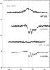 |
Fig. B.2 As Fig. B.1, toward IRAS 16272. |
| In the text | |
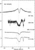 |
Fig. B.3 As Fig. B.1, toward NGC 6334I(N). |
| In the text | |
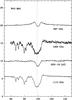 |
Fig. B.4 As Fig. B.1, toward W43 MM1. |
| In the text | |
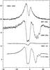 |
Fig. B.5 As Fig. B.1, toward DR21(OH). |
| In the text | |
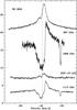 |
Fig. B.6 As Fig. B.1, toward W3 IRS5. |
| In the text | |
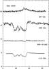 |
Fig. B.7 As Fig. B.1, toward IRAS 18089. |
| In the text | |
|
Fig. B.8 As Fig. B.1, toward W33A. The emission/absorption feature near 0 km s-1 in the 1669 GHz spectrum is the H2O 1661 GHz line from the other sideband. |
| In the text | |
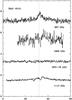 |
Fig. B.9 As Fig. B.1, toward IRAS 18151. |
| In the text | |
|
Fig. B.10 As Fig. B.1, toward AFGL 2591. The emission feature near +18 km s-1 in the 1669 GHz spectrum is the H2O 1661 GHz line from the other sideband. |
| In the text | |
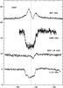 |
Fig. B.11 As Fig. B.1, toward G 327. |
| In the text | |
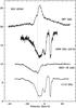 |
Fig. B.12 As Fig. B.1, toward NGC 6334I. |
| In the text | |
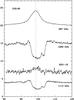 |
Fig. B.13 As Fig. B.1, toward G29.96. |
| In the text | |
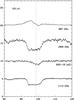 |
Fig. B.14 As Fig. B.1, toward G31.41. |
| In the text | |
|
Fig. B.15 As Fig. B.1, toward G5.89. The emission feature near +90 km s-1 in the H |
| In the text | |
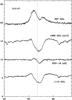 |
Fig. B.16 As Fig. B.1, toward G10.47. |
| In the text | |
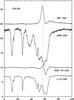 |
Fig. B.17 As Fig. B.1, toward G34.26. |
| In the text | |
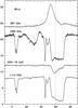 |
Fig. B.18 As Fig. B.1, toward W51e. |
| In the text | |
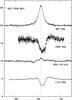 |
Fig. B.19 As Fig. B.1, toward NGC 7538 IRS1. |
| In the text | |
|
Fig. C.1 Continuum model for IRAS 05358. Top left: spectral energy distribution. Top right: submillimeter image with 3σ contour marked in white and useable map sectors marked in black. Bottom left: temperature and density structure as a function of radius. Bottom right: submillimeter emission profiles. The numbers in the top left panel are the modeled envelope mass, the modeled luminosity, the adopted envelope size and the adopted distance. |
| In the text | |
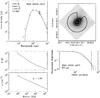 |
Fig. C.2 As Fig. C.1, for IRAS 16272. |
| In the text | |
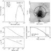 |
Fig. C.3 As Fig. C.1, for NGC 6334I(N). |
| In the text | |
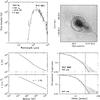 |
Fig. C.4 As Fig. C.1, for W43-MM1. |
| In the text | |
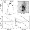 |
Fig. C.5 As Fig. C.1, for DR21(OH). |
| In the text | |
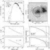 |
Fig. C.6 As Fig. C.1, for W3 IRS5. |
| In the text | |
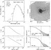 |
Fig. C.7 As Fig. C.1, for IRAS 18089. |
| In the text | |
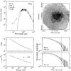 |
Fig. C.8 As Fig. C.1, for W33A. |
| In the text | |
 |
Fig. C.9 As Fig. C.1, for IRAS 18151. |
| In the text | |
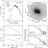 |
Fig. C.10 As Fig. C.1, for AFGL 2591. |
| In the text | |
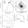 |
Fig. C.11 As Fig. C.1, for G327–0.6. |
| In the text | |
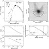 |
Fig. C.12 As Fig. C.1, for NGC 6334I. |
| In the text | |
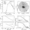 |
Fig. C.13 As Fig. C.1, for G29.96. |
| In the text | |
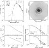 |
Fig. C.14 As Fig. C.1, for G31.41. |
| In the text | |
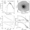 |
Fig. C.15 As Fig. C.1, for G5.89. |
| In the text | |
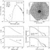 |
Fig. C.16 As Fig. C.1, for G10.47. |
| In the text | |
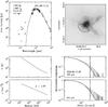 |
Fig. C.17 As Fig. C.1, for G34.26. |
| In the text | |
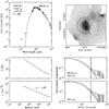 |
Fig. C.18 As Fig. C.1, for W51e. |
| In the text | |
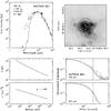 |
Fig. C.19 As Fig. C.1, for NGC 7538 IRS1. |
| In the text | |
|
Fig. D.1 Observed line fluxes (positive: emission) or absorbances (negative: absorption) versus bolometric luminosity L of the source (top), versus envelope mass M (middle), and versus the ratio L/M (bottom). Open squares: mid-IR-quiet HMPOs; filled squares: mid-IR-bright HMPOs; triangles: hot molecular cores; circles: ultracompact Hii regions. Uncertainties in line fluxes are ≈10%, while the typical uncertainty of masses, luminosities and L/M ratios is a factor of 2. |
| In the text | |
 |
Fig. D.2 As Fig. D.1, for the narrow outflow component. |
| In the text | |
 |
Fig. D.3 As Fig. D.1, for the broad outflow component. |
| In the text | |
|
Fig. D.4 Line width of the narrow outflow component versus bolometric luminosity L of the source (top), versus envelope mass M (middle), and versus the ratio L/M (bottom). The error bar denotes the typical uncertainty in mass, luminosity, and L/M ratio; the uncertainty in line width is smaller than the symbol size. |
| In the text | |
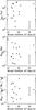 |
Fig. D.5 As Fig. D.4, for the broad outflow component. |
| In the text | |
Current usage metrics show cumulative count of Article Views (full-text article views including HTML views, PDF and ePub downloads, according to the available data) and Abstracts Views on Vision4Press platform.
Data correspond to usage on the plateform after 2015. The current usage metrics is available 48-96 hours after online publication and is updated daily on week days.
Initial download of the metrics may take a while.