| Issue |
A&A
Volume 552, April 2013
|
|
|---|---|---|
| Article Number | A44 | |
| Number of page(s) | 10 | |
| Section | Extragalactic astronomy | |
| DOI | https://doi.org/10.1051/0004-6361/201220754 | |
| Published online | 21 March 2013 | |
The interaction-driven starburst contribution to the cosmic star formation rate density
INAF – Osservatorio Astronomico di Roma, via di Frascati 33,
00040
Monte Porzio Catone,
Italy
e-mail:
This email address is being protected from spambots. You need JavaScript enabled to view it.
Received:
16
November
2012
Accepted:
6
February
2013
Abstract
An increasing amount of observational evidence supports the notion that there are two modes of star formation: a quiescent mode in disk-like galaxies and a starburst mode, which is generally interpreted as driven by merging. Using a semi-analytic model of galaxy formation, we derive the relative contribution to the cosmic star formation rate density of quiescently star forming and starburst galaxies, predicted under the assumption that starburst events are triggered by galaxy encounters (merging and fly-by kind) during their merging histories. We show that, within this framework, quiescently star forming galaxies dominate the cosmic star formation rate density at all redshifts. The contribution of the burst-dominated star forming galaxies increases with redshift, starting from ≲5% at low redshift (z ≲ 0.1) to ~20% at z ≥ 5. We estimated that the fraction of the final (z = 0) galaxy stellar mass that is formed through the burst component of star formation is ~10% for 1010 M⊙ ≤ M∗ ≤ 1011.5 M⊙. Selected according to their distance from the galaxy main sequence, starburst galaxies account for ~10% of the star formation rate density in the redshift interval 1.5 < z < 2.5, i.e., at the cosmic peak of the star formation activity.
Key words: galaxies: evolution / galaxies: fundamental parameters / galaxies: interactions / galaxies: starburst
© ESO, 2013
1. Introduction
How galaxies build up their stellar mass is a central question in galaxy formation. Many previous works have demonstrated that a substantial fraction (30–50%) of the stellar mass formed between z ~ 3 and z ~ 1 (Dickinson et al. 2003; Fontana et al. 2003, 2004, 2006; Glazebrook et al. 2004; Drory et al. 2004; Rudnick et al. 2006; Papovich et al. 2006; Yan et al. 2006; Pozzetti et al. 2007). However, it is still unclear what the major channel for galaxy growth is during this period. Two star formation modes have been identified: the first is a “quiescent”1 mode in disk-like galaxies where the star formation is extended over the whole galaxy disk and which occurs on time scales of ~(1−2) Gyr; the second is a compact, starburst mode, where the star formation tends to be dominated by the nuclear regions, and the gas depletion time scales are significantly lower (~107−108 yr) than those in quiescently star forming galaxies.
This accelerated mode of star formation is very likely triggered by major mergers, as suggested by observational evidence and theoretical arguments. Observationally, major mergers are associated with enhancements in star formation in local ultra luminous infrared galaxies (ULIRGs, Sanders & Mirabel 1996; Elbaz et al. 2007), and some sub-millimetre galaxies (SMGs, Tacconi et al. 2008; Daddi et al. 2007, 2009; Engel et al. 2010). On the theoretical side, the merger-driven scenario for starburst galaxies is supported by the results of high-resolution numerical simulations, which show the effectiveness of galaxy major mergers in causing the loss of angular momentum of the gas in the galaxy disk, with the consequent trigger of starburst events into the central regions of the galaxy (Hernquist 1989; Barnes & Hernquist 1991, 1996; Mihos & Hernquist 1994, 1996). It is also supported by the success of semi-analytic models (SAMs) of galaxy formation, which include this additional channel of star formation, in reproducing the early formation of stars in massive galaxies (e.g. Somerville et al. 2001; Menci et al. 2004, 2005).
An effective tools for understanding the relative contribution of the different star formation modes is provided by the scaling relations connecting the star formation rate (SFR) with global galactic quantities, such as the gas mass (the Schmidt-Kennicutt relation) or the total stellar mass (M∗). In fact, the normalization and/or the scaling of the SFR with such quantities differs for starbursts and quiescently star forming galaxies. As regards the former, the extension of the well-established local relation (Kennicutt 1998) to higher redshifts has shown that quiescently star forming galaxies follow the local Schmidt-Kennicutt relation, while the SFRs of starburst galaxies are typically one order of magnitude greater than expected from their projected gas surface density (Daddi et al. 2010; Genzel et al. 2010). As regards the correlation between the SFR and M∗, it has recently been shown that quiescently star forming galaxies lie along a “main sequence” characterized by a typical redshift-dependent value of the specific star formation rate (SSFR = SFR/M∗), while the less numerous starburst population is characterized by higher values of the SSFR. The main sequence is observed over a wide range of redshifts, from z ~ 0 to z ~ 6, and it is characterized by a small scatter (~0.3 dex), by a normalization that increases by a factor of ~20 from z ≃ 0 to z ≃ 2, and by a slope that is sensitive to the technique used to select the sample of star forming galaxies and to the procedure for measuring M∗ and SFR, with values ranging from 0.6 to 1 (Brinchmann et al. 2004; Noeske et al. 2007; Elbaz et al. 2007; Daddi et al. 2007, 2009; Santini et al. 2009; Salim et al. 2007; Stark et al. 2009; González et al. 2011).
The techniques for measuring the SFRs and the stellar masses in galaxies are based on different observational tracers. A fruitful approach to estimating the stellar mass is the SED fitting. This technique is based on comparing a grid of spectral templates computed from standard spectral synthesis models and the available multi wavelength photometry (Papovich et al. 2001; Shapley et al. 2001, 2005; Fontana et al. 2006; Santini et al. 2009). However, such a method does not provide reliable star formation histories (SFHs) at high redshifts, where the uncertainties become larger due to the SFR-age-metallicity degeneracies. An alternative commonly used estimator of the SFR is the UV rest-frame band, where young and massive stars emit most of their light. Here the drawback is that dust absorbs, reprocesses, and re-radiates UV photons at near-to-far IR wavelengths, so that reliability of UV luminosity as an SFR tracer depends on large and uncertain corrections relying upon the dust properties. Since most of the energy radiated by newly formed stars is reprocessed by dust, to accurately derive the SFR, it is necessary to determine the dust bolometric output. In the past, the total IR luminosity (from 8 to 1000 μm) was calculated by extrapolating observation in the mid-IR. With the launch of the Herschel Space Observatory (Pilbratt et al. 2010), it has now become possible to measure the far-IR luminosity of distant galaxies at wavelengths where the dust emission is known to peak.
A recent study based on Herschel observations of star forming galaxies at 1.5 < z < 2.5 indicates that only ~2% of massive (M∗ > 1010 M⊙) galaxies in this sample have a starburst nature, and they account for only ~10% of the star formation rate density (SFRD) at z ~ 2 (Rodighiero et al. 2011). This finding represents a test case for the merger-driven scenario for starburst galaxies, since in this framework the occurrence of the starburst events is driven by the galaxy merger rates, which are expected to increase with redshift. In this paper we investigate this issue in the framework of a theoretical model of galaxy formation that includes a physical description of starburst triggered by galaxy interactions during their merging histories. The latter are described through Monte Carlo realizations, and are connected to gas processes and star formation using a semi-analytic model of galaxy formation in a cosmological framework (Menci et al. 2004, 2005, 2006, 2008). In our model the starburst events are triggered not only by galaxy major mergers (i.e. the fusion of galaxies with comparable mass, m ≈ m′) but also by minor mergers (m ≪ m′) and by closer galaxy interactions that do not lead to bound merging (fly-by events). Minor mergers and fly-by events induce starburst with a lower efficiency than for major mergers, but they are more probable, so they contribute appreciably to the cosmic SFH.
A description of the SAM is given in Sect. 2; in Sect. 3 we derive the predicted SFR-M∗ relation at 1.5 < z < 2.5 and the contribution to the cosmic SFRD of starbursts and quiescently star forming galaxies; discussions and conclusions follow in Sects. 4 and 5.
2. The model
We use the SAM described in details in Menci et al. (2004, 2005, 2006, 2008), which connects, within a cosmological framework, the baryonic processes (gas cooling, star formation, supernova feedback) to the merging histories of the dark matter (DM) haloes. AGN activities, triggered by galaxy interactions in common DM haloes, and the related feedback processes are also included. Here we recall the basic points.
2.1. The dark matter merging trees
Galaxy formation and evolution is driven by the collapse and growth of DM haloes, which develop from the gravitational instability of overdense regions in the primordial DM density field. This is taken to be a random, Gaussian density field with cold dark matter (CDM) power spectrum within the “concordance cosmology” (Spergel et al. 2007) for which we adopt round parameters ΩΛ = 0.7, Ω0 = 0.3, baryonic density Ωb = 0.04, and Hubble constant (in units of 100 km s-1 Mpc-1) h = 0.7. The normalization of the spectrum is taken to be σ8 = 0.9 in terms of the variance of the field smoothed over regions of 8 h-1 Mpc.
As cosmic time increases, larger and larger regions of the density field collapse and eventually lead to the formation of groups and clusters of galaxies; previously formed, galactic size condensations are enclosed. The merging rates of the DM haloes are provided by the Extended Press & Schechter formalism (see Bond et al. 1991; Lacey & Cole 1993). The clumps included in larger DM haloes may survive as satellites, or merge to form larger galaxies due to binary aggregations, or coalesce into the central dominant galaxy due to dynamical friction. These processes take place in time scales that grow longer over cosmic time, so the number of satellite galaxies increases as the DM host haloes grow from groups to clusters (see Menci et al. 2005, 2006).
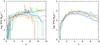 |
Fig. 1 SFHs drawn from the Monte Carlo realizations of galaxies, which, at z = 0, have masses of M∗ ≃ 1010 M⊙ (left) and M∗ ≃ 1012 M⊙ (right). The SFHs are obtained by summing over all the progenitors that have merged to form galaxies of the selected final mass. The quiescent star formation is represented by the smooth component of the SFHs, the burst component by the impulsive one. The duration of the SFR-excess phase due to the interactions is represented by the width of the peak of the SFHs. |
2.2. The star formation law
The processes connecting the baryonic components to the growing DM haloes (with mass m) are computed as follows. Starting from an initial amount mΩb/Ω of gas at virial temperature of the galactic haloes, we compute the mass mc of cold baryons within the cooling radius. The cooled gas mass mc settles into a rotationally supported disk with radius rd (typically ranging from 1 to 5 kpc), rotation velocity vd, and dynamical time td = rd/vd, all computed after Mo et al. (1998). Two channels of star formation may convert part of such gas into stars:
-
i)
quiescent star formation, corresponding to the gradualconversion of the cold gas in the galaxy disk into stars, forwhich we assume the canonical Schmidt-Kennicutt form:
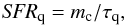 (1)where
τq = qtd,
and q is a model free parameter that is chosen to match the Kennicutt (1998) relation;
(1)where
τq = qtd,
and q is a model free parameter that is chosen to match the Kennicutt (1998) relation; -
ii)
burst-like star formation triggered by galaxy interactions, at a rate
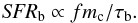 (2)
(2)
 (3)where b
is the impact parameter, evaluated as the greater of the radius
rd and the average distance of the galaxies in the halo,
m′ is the mass of the partner galaxy in the interaction,
Vrel is the relative velocity between galaxies, and the
average runs over the probability of finding such a galaxy in the same halo where the
galaxy with mass m is located. The pre-factor accounts for the
probability 1/2 of inflow rather than outflow related to the sign of Δj.
We assume the value of 3/4 for the proportionality constant in Eq. (2), while the remaining fraction of the inflow
is assumed to feed the central black hole (see Sanders
& Mirabel 1996). When applied to the black hole accretion and to the
related AGN emission, the above model has proven to be very successful in reproducing the
observed properties of the AGN population from z = 6 to the present
(Menci et al. 2004, 2008; Lamastra et al. 2010).
(3)where b
is the impact parameter, evaluated as the greater of the radius
rd and the average distance of the galaxies in the halo,
m′ is the mass of the partner galaxy in the interaction,
Vrel is the relative velocity between galaxies, and the
average runs over the probability of finding such a galaxy in the same halo where the
galaxy with mass m is located. The pre-factor accounts for the
probability 1/2 of inflow rather than outflow related to the sign of Δj.
We assume the value of 3/4 for the proportionality constant in Eq. (2), while the remaining fraction of the inflow
is assumed to feed the central black hole (see Sanders
& Mirabel 1996). When applied to the black hole accretion and to the
related AGN emission, the above model has proven to be very successful in reproducing the
observed properties of the AGN population from z = 6 to the present
(Menci et al. 2004, 2008; Lamastra et al. 2010).
The probability that a given galaxy is in a burst phase is defined as the ratio
τb/τr of the
duration of the burst to the average time interval between bursts. The rate of such
encounters  is
is 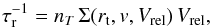 (4)where
nT = 3NT/4πR3
is the number density of galaxies in the same halo, Vrel their
relative velocity, and
(4)where
nT = 3NT/4πR3
is the number density of galaxies in the same halo, Vrel their
relative velocity, and  the cross section for such
encounters, which is given by Saslaw (1985) in
terms of the tidal radius rt associated to a galaxy with given
circular velocity v (see Menci et al.
2004).
the cross section for such
encounters, which is given by Saslaw (1985) in
terms of the tidal radius rt associated to a galaxy with given
circular velocity v (see Menci et al.
2004).
At each time step, the mass Δmh returned
from the cold gas content of the disk to the hot gas phase owing to the energy released by
SNae following star formation is estimated from canonical energy balance arguments as
 , where
Δm∗ is the stellar mass formed in the time step,
η0 is the number of SNe per unit solar mass (for a Salpeter
initial mass function
η0 = 6.5 × 10⁻³ M⊙-1),
ESN = 1051 erg/s is the
energy of ejecta of each SN, vc the circular velocity of the
galactic halo, and ϵ0 = 0.01 is a tunable efficiency for the
coupling of the emitted energy with the cold interstellar medium. At each merging event,
the masses of the different baryonic phases (Δmc,
Δm∗ and Δmh) in
each galaxy are refuelled by those in the merging partners. Thus, for each galaxy the star
formation is driven by the cooling rate of the hot gas and by the rate of refuelling of
the cold gas, which in turn is intimately related to the galaxy merging histories. The
model has been tested against several observed properties of the local galaxy population
like the B band luminosity function, the stellar mass function, the
Tully-Fisher relation, the galaxy bimodal colour distribution, and the distribution of
cold gas and disk sizes. At higher redshifts, the model has been tested against the
evolution of the luminosity functions and the number counts in different bands (Menci et al. 2005, 2006).
, where
Δm∗ is the stellar mass formed in the time step,
η0 is the number of SNe per unit solar mass (for a Salpeter
initial mass function
η0 = 6.5 × 10⁻³ M⊙-1),
ESN = 1051 erg/s is the
energy of ejecta of each SN, vc the circular velocity of the
galactic halo, and ϵ0 = 0.01 is a tunable efficiency for the
coupling of the emitted energy with the cold interstellar medium. At each merging event,
the masses of the different baryonic phases (Δmc,
Δm∗ and Δmh) in
each galaxy are refuelled by those in the merging partners. Thus, for each galaxy the star
formation is driven by the cooling rate of the hot gas and by the rate of refuelling of
the cold gas, which in turn is intimately related to the galaxy merging histories. The
model has been tested against several observed properties of the local galaxy population
like the B band luminosity function, the stellar mass function, the
Tully-Fisher relation, the galaxy bimodal colour distribution, and the distribution of
cold gas and disk sizes. At higher redshifts, the model has been tested against the
evolution of the luminosity functions and the number counts in different bands (Menci et al. 2005, 2006).
3. Results
3.1. The SFR-M∗ relation
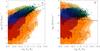 |
Fig. 2 Left: SFR-M∗ relation at 1.5 < z < 2.5. The five filled contours correspond to equally spaced values of the density (per Mpc3) of model galaxies in logarithmic scale: from 10-6 for the lightest filled region to 10-2 for the darkest. Green squares: Herschel-PACS- selected galaxies, black circles: BzK galaxies, from the Rodighiero et al. (2011) sample; blue triangles: GOODS-MUSIC catalogue from the Santini et al. (2009) sample. The dashed and long-dashed lines indicate the best-fit of the galaxy main sequence obtained by Rodighiero et al. (2011) and Santini et al. (2009) respectively, while the solid line shows the spline fit to the peaks of the SFR distributions of model galaxies as a function of stellar mass. Right: SSFR as a function of M∗. Colour code, symbols, and solid line as in the left panel. The dashed and thin solid lines respectively indicate the SSFR > SSFRMS − 2σ and the SSFR > tH(z)-1 limits of the galaxy samples used in the analysis of Sect. 3.2. |
As a first step in studying the contribution of starbursts and quiescently star forming galaxies to the cosmic SFRD, we compare the predicted SFR-M∗ (left) and SSFR-M∗ (right) relations in Fig. 2 for model galaxies with M∗ > 109.5 M⊙ at 1.5 < z < 2.5 with those obtained by Rodighiero et al. (2011) and by Santini et al. (2009). The former authors used a combination of BzK- and Herscel-PACS- selected star forming galaxies from the COSMOS and GOODS fields. The BzK colour selection is designed to identify star forming galaxies in the redshift interval 1.5 < z < 2.5 by using colours that sample key features in the spectral energy distributions of galaxies, mainly the rest-frame 4000 Å break and the UV continuum slope (BzK ≡ (z − K)AB − (B − z)AB ≥ −0.2, Daddi et al. 2004). The SFRs of BzK galaxies are estimated from the UV-rest-frame luminosity corrected for dust reddening, and they yield an almost linear correlation with the stellar mass. The Herschel-PACS detection limit depends on redshift; at z ≃ 2 it corresponds to ~200 M⊙/yr and to ~50 M⊙/yr for the COSMOS and GOODS fields, respectively. The PACS-based SFRs run almost flat with the stellar mass and occupy the upper envelop of the distribution. This different behaviour could be ascribed to the differences in how the two samples were selected, one being SFR limited and the other mass limited (Rodighiero et al. 2011). The Santini et al. (2009) sample is based on the GOODS-MUSIC catalogue; for detected sources, the SFRs are derived from the 24 μm emission, corrected to consider the well-known overestimation of the SFR for bright sources at z ~ 2 (see Santini et al. 2009, for further details), while for undetected objects the SFRs are derived from SED fitting in the optical/near-IR range. In contrast to the previous sample, this catalogue includes passive galaxies, and this explains the larger extension of the SFR-M∗ relation towards low SFRs. These data lie in the predicted confidence region represented by the contour plot; however, the bottom-left part of the SFR-M∗ diagram remains unsampled due to observational incompleteness. This observational limitation did not allow us to test one of the striking feature of the SFR-M∗ relation predicted by hierarchical models of galaxy formation, namely, the behaviour of the scatter. In fact, its increase with decreasing stellar mass is due to the wide variety of SFHs corresponding to the low-mass population, while the similarity of the SFHs of high-mass galaxies results in smaller scatter in the SFR-M∗ plane. This is especially true at high redshifts z > 6. At such an epoch, the small number of progenitors of present-day low-mass galaxies (and their different collapse time) yield a large variance in the SFHs, while the larger number of progenitors of high-mass galaxies (already collapsed since they formed in biased regions of the density field) result in a smaller variance among the different SFHs (see Fig. 1).
Figure 2 indicate the best-fit of the galaxy main sequence obtained by Rodighiero et al. (2011) and Santini et al. (2009) and the spline fit to the peaks of the SFR (SSFR) distributions of model galaxies as a function of stellar mass (log SFR = 0.8 ∗ log M∗ − 7.5). The slopes of the observed and predicted SFR-M∗ relations are similar (0.8 ≤ α ≤ 0.9), while the normalization of the predicted relation is a factor of four to five lower than the observed relations. The offset between the predicted and observed SFR-M∗ relations in the local universe (z ≃ 0.1 Brinchmann et al. 2004) reduces by a factor of about two, implying that the evolution of the SSFR with redshift predicted by the model is slower than observed at z ≲ 2. The local distribution of model galaxies in the SFR-M∗ plane shows bimodal behaviour, with a clear separation between actively star forming and passively evolving galaxies, as seen in observations (Brinchmann et al. 2004).
Similar offsets between the observed SFR-M∗ relation and those expected by various kind of SAMs and hydrodynamical simulations has been previously reported in the literature (see e.g. Daddi et al. 2007; Davé 2008; Fontanot et al. 2009; Damen et al. 2009; Santini et al. 2009; Lin et al. 2012). Understanding whether this mismatch comes from systematic effects in the stellar mass and/or SFR determinations, or from the incompleteness in our basic picture of galaxy assembly is a very difficult task. The amplitude of this offset depends on the the technique used to estimate the SFR and stellar mass and on the sample selection (see the offset between the dashed and long-dashed lines). In our analysis of the role of starbursts relative to quiescently star forming galaxies (Sect. 3.2) we normalize both the model and observed SFRs to their main sequence values, and we address this mismatch in more detail in Sect. 4.
To understand the role of starbursts and quiescently star forming galaxies in deriving the SFR-M∗ relation we separately show in Fig. 3 the relations obtained by selecting from the Monte Carlo simulations galaxies dominated by the quiescent mode of star formation (SFRq > SFRb, left panel), and galaxies dominated by the burst mode of star formation (SFRb > SFRq, right panel).
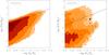 |
Fig. 3 Predicted SFR-M∗ relation at 1.5 < z < 2.5 obtained by selecting from the model galaxies dominated by the quiescent (left) and burst (right) mode of star formation. Contours and solid line as in Fig. 2. |
The former show a tight correlation between the SFR and the stellar mass. This is a natural outcome, because this component is a fairly steady function of time (see the smooth component of the SFHs in Fig. 1). The scatter of this relation originates in the distribution of cold gas at a given stellar mass, and ultimately stems from the stochastic nature of the merging histories of galaxies. When we select galaxies where SFRb > SFRq we obtain a more scattered distribution in the SFR-M∗ plane. In these galaxies the SFR is not only determined by the amount of cold gas available in the galaxy disk, but also regulated by the amount of this gas, which is destabilized during galaxy interactions (see Eq. (2)). Minor mergers and fly-by events, which dominate the statistics of encounters in the hierarchical clustering scenario, induce a lower fraction of destabilized gas compared to major mergers. (Note the dependence of f on the mass ratio m′/m in Eq. (3)). This analysis shows that the main sequence is mainly populated by quiescently star forming galaxies, and the loci well above and below it by galaxies experiencing major mergers and minor mergers/fly-by events, respectively.
3.2. The contribution of starbursts and quiescently star forming galaxies to the cosmic SFRD
We now quantify the results shown in the previous section, and derive the relative contribution of starbursts and quiescently star forming galaxies to the cosmic SFRD and comoving number density in the redshift interval 1.5 < z < 2.5. To perform a quantitative comparison, we first need to define the sample of model star forming galaxies. Since the observational results we compare with are derived from a combination of samples adopting different criteria to select star forming galaxies (see Sect. 3.1), we have performed two different selections of model galaxies in order to reproduce the observational selection effects, at least partially. The first corresponds to model galaxies with SSFR > SSFRMS − 2σ (Fig. 2b), where SSFRMS is the value obtained for model galaxies and σ = 0.3 dex is the scatter of the observed SFR-M∗ relation (Rodighiero et al. 2011; Daddi et al. 2004). The second corresponds to model galaxies with SSFR > tH(z)-1 (line in Fig. 2b that indicates the corresponding SSFR value at z = 2), which select galaxies whose current SFR is stronger than its average past SFR (see e.g. Fontana et al. 2009). Within these samples, we derived the distributions of SSFR normalized to the value of main sequence galaxies (SSFRMS), in four equally spaced stellar mass bins from M∗ = 1010 M⊙ to M∗ = 1011.5 M⊙ (see Fig. 4). According to Rodighiero et al. (2011), the galaxies observationally classified as starburst are those with SSFRSB > 4 × SSFRMS (Fig. 4).
 |
Fig. 4 SSFR distributions of model galaxies, at 1.5 < z < 2.5, in four mass bins. The blue histograms refer to galaxies dominated by the quiescent mode of star formation, the red histograms to galaxies dominated by the burst mode of star formation, and the green histograms to galaxies with an interaction-driven star formation component. The solid vertical lines show the position of the main sequence, while the vertical dotted lines show the SSFR threshold used to identify starburst galaxies: SSFRSB > 4 × SSFRMS. The solid distributions are obtained by selecting galaxies with SSFR > tH(z)-1, while dashed distributions are obtained selecting galaxies with SSFR > SSFRMS − 0.6 dex. |
We then proceeded to assess how galaxies observationally classified as starburst compare with model galaxies. To this aim, we separately derived the distributions of model galaxies dominated by the quiescent mode of star formation and of galaxies dominated by the burst mode of star formation. We find that the threshold SSFRSB > 4 × SSFRMS used by Rodighiero et al. (2011) is indeed effective in filtering out quiescent galaxies, independently of the criterion adopted to define our sample of star forming galaxies; in fact, in the model SSFR values above this threshold are obtained only through the burst component of the star formation. However, this criterion fails to select a considerable part of the burst-dominated star forming galaxies where the galaxy interactions do not boost the SFRs above the quiescent values (minor mergers and fly-by events). The above results enlighten the physical difference between galaxies observationally classified as starbursts and galaxies with an interaction-driven star formation component. The latter also include galaxies not dominated by the burst mode of star formation, as indicated by the distributions of galaxies with a burst component of star formation (SFRb > 0, Fig. 4). In the following we derive the relative contribution to the comoving number density and to the cosmic SFRD in the redshift range 1.5 < z < 2.5 for all these classes of star forming galaxies: (i) main sequence galaxies (SFRq > SFRb); (ii) starburst galaxies (SSFRSB > 4 × SSFRMS); (iii) burst-dominated star forming galaxies (SFRb > SFRq); and (iv) galaxies with an interaction-driven star formation component (SFRb > 0).
The predicted relative contribution of the above classes of galaxies to the comoving number density of star forming galaxies is shown in Fig. 5a. The fraction of starbursts and burst-dominated galaxies with respect to the total number of star forming galaxies is compared with the observational results by Rodighiero et al. (2011). While the predicted fraction of starburst galaxies remains around NSB/NMS + SB ~ 1%, the exact values predicted by the model depend on the criteria adopted to define the global sample of star forming galaxies (i.e., NMS + SB), defining the upper and the lower envelopes of both these regions. The lower fraction of starburst galaxies obtained with the selection SSFR > SSFRMS-2σ compared to the selection SSFR > tH(z)-1 is due to the larger number of “on-sequence” galaxies selected in the first case (especially for high masses, see Fig. 4), while the number of galaxies NSB almost remains unchanged.
The figure shows that, even in a hierarchical model connecting the physics of galaxies to their merging histories, the fraction of galaxies classified as starburst remains within values ~1%, even lower than the observational values (~2%); values around 2–3% are obtained when burst-dominated galaxies are considered. This is for two reasons: i) in hierarchical models, the statistics of merging events is dominated by minor episodes that do not produce SSFR above the threshold adopted in the observations; ii) the duration of bursts t ≈ 107−108 yrs is much shorter than the typical time scale between two encounters, so that the probability of finding a galaxy in a starburst phase is correspondingly low. As regards the former point i), we show in Fig. 5a the fraction of the galaxy population with a star formation component induced by galaxy interactions, SFRb > 0. When all galaxy interactions are considered, including minor merging and fly-by, the fraction of galaxies with an interaction-driven star formation component increases with M∗ to reach values ≈10-1. The trend with M∗ is due to the larger cross section for interactions of massive galaxies (see Eq. (4)) and to massive galaxies being found in dense environments with an enhanced galaxy interaction rate. The merging histories of massive galaxies are dominated by minor merging events that are less effective in destabilizing the gas in the galaxy disks (see Eq. (3)), therefore a lower number of massive galaxies satisfy the SFRb > SFRq criterion, and this explains the flattening of the hatched and shaded regions with increasing stellar mass in Fig. 5a.
As regards the starburst duty cycle, the above value ~10-1 of the fraction of galaxies with SFRb > 0 implies a value τb/τr ~ 0.1 for the ratio of the burst duration τb over the interaction time scale τr (see Sect. 2.2). This is indeed what is expected from both theoretical arguments and observational hints. In fact, the interaction time scale τr = (n Σ V)-1 can be estimated by assuming a simple geometrical cross section Σ ≈ πr2. For typical values of the galaxy gravitational radius r ~ 0.1 Mpc and of the galaxy relative velocities V ~ 100 km s-1, and assuming a density of a few galaxies per Mpc3, we obtain an estimate τr ~ 109 yr. When compared with the galaxy crossing time (determining the duration of bursts, see Sect. 2.2) τb ~ 108 yr, a value τb/τr ≈ 0.1 is obtained for the duty cycle, as expected. This value is also consistent with the duty cycle of AGN measured at z ≈ 1–2 with luminosity L ≳ 1043 erg/s (Martini et al. 2009; Eastman et al. 2007), as expected in our framework where both starbursts and AGNs are triggered by galaxy interactions.
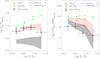 |
Fig. 5 Left: fraction of starburst (shaded region), burst-dominated (hatched region), and interacting (triangles) galaxies as function of the stellar mass at 1.5 < z < 2.5. Right: contribution to the cosmic SFRD of the same classes of star forming galaxies. The lines indicate the model predictions when adopting the SSFR > tH(z)-1 (solid lines) and the SSFR > SSFRMS-2σ (dashed lines) criterion to define the global sample of star forming galaxies. The data points indicate the results obtained by Rodighiero et al. (2011) for starburst galaxies (SSFR > 4 × SSFRMS). |
We now estimate the contribution of the different classes of star forming galaxies to the cosmic SFRD at 1.5 ≤ z ≤ 2.5, shown in Fig. 5b. The interaction-driven scenario predicts that the contribution of the entire interacting galaxy population is ~15% irrespective of stellar mass. At lower stellar masses, this quantity is mainly contributed by burst-dominated galaxies, while at higher stellar masses the contribution of the quiescent mode of star formation becomes important, as indicated by the decrease in the ratio SFRDSB/SFRDMS + SB with increasing M∗ for the SFRb > SFRq and SSFRSB> 4 × SSFRMS populations. In fact, for the burst-dominated star forming galaxy population, the contribution to the cosmic SFRD is ~15% for M∗ ~ 1010 M⊙ and (6–10)% for M∗ ~ 1011.5 M⊙, and for starburst galaxies it is slightly lower: ~12% for M∗ ~ 1010 M⊙ and (4–6)% for M∗ ~ 1011.5 M⊙. Therefore, this scenario is consistent with the observational finding that the cosmic SFRD in the redshift range 1.5 < z < 2.5 is mainly contributed by quiescently star forming galaxies (Rodighiero et al. 2011). However, it must be noted that, given the lower fraction of starburst galaxies predicted by the model, the match between the predicted and observed starburst contributions is determined by the lower value of the SFR of model main sequence galaxies (see Fig. 2).
Since the burst mode of star formation is intimately related to the galaxy interaction
rate, which is expected to increase with redshift, we investigate how these contributions
change as a function of the cosmic epoch. To address this issue, we derive the
contribution to the cosmic SFRD of quiescent-dominated and burst-dominated systems
separately as a function of redshift (Fig. 6). We
find that quiescent systems dominate the global SFRD at all redshifts. However, the
contribution of the burst-dominated population increases with redshift, rising from ≲5% at
low redshift (z ≲ 0.1) to ~20% at z ≳ 5. This is a
typical feature of the hierarchical clustering scenario where the starburst events are
triggered by galaxy interaction during their merging histories. A similar evolution was
obtained by Hopkins et al. (2010) on the basis of
cosmological hydrodynamical simulations. The physical origin of this behaviour can be
understood as follows: at high redshift, both the interaction rate
(Eq. (4)) and the fraction of destabilized
gas f (Eq. (3)) are high,
the former because of the high densities, the latter owing to the high ratio
m′/m ≈ 1 characteristic
of this early phase (z ≳ 3) when galaxy interactions mainly involve
partners with comparable mass (major mergers). At lower z, the decline in
the interaction rate and in the destabilized gas fraction suppresses the burst mode of
star formation, thus lowering its contribution to the total SFRD.
An immediate implication of the above is that the fraction of the stellar mass formed through the SFR associated with the destabilized cold gas during galaxy interactions increases with redshift. This is illustrated in Fig. 7, where the contours show the average values of the ratio Mburst(z)/M∗(z) as a function of M∗ and z. The mass Mburst(z) is the stellar mass that a galaxy has formed through the burst mode of star formation up to that redshift, and M∗(z) is the total galaxy stellar mass at that z. From this figure one can infer that ~10% of the final (z = 0) galaxy stellar mass has been formed during bursts for 1010 M⊙ ≤ M∗ ≤ 1011.5 M⊙. At higher redshift (z ≳ 4) this fraction increases up to ~20%. To illustrate how the ratio Mburst(z)/M∗(z) varies during the formation of galaxies with different final masses, we also show the growth histories of typical galaxies with final mass: M∗(z = 0) = 1012 M⊙, M∗(z = 0) = 1011 M⊙, and M∗(z = 0) = 1010 M⊙ (Fig. 7).
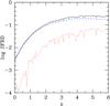 |
Fig. 6 Contribution to the cosmic SFRD of galaxies with SFR ≥ 1.4 × 10⁻⁶ M⊙/yr (corresponding to UV luminosity LUV ≳ 1015 W Hz−1 when adopting the calibration given in Kennicutt 1998) as a function of redshift (solid line). Dashed line indicates the contribution of galaxies dominated by the quiescent mode of star formation, while dotted line indicates the contribution of galaxies dominated by the burst mode of star formation. |
These paths illustrate that at high redshift (z ≳ 2) and for massive objects, high values of Mburst(z)/M∗(z) are expected, since such massive galaxies formed in biased regions of the density field where high-redshift interactions are extremely effective in triggering starbursts. For less massive galaxies the high-redshift value of the Mburst(z)/M∗(z) ratio progressively lowers, since these galaxies formed in less dense environments.
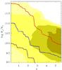 |
Fig. 7 Predicted average values of the ratio Mburst(z)/M∗(z) as a function of redshift and galaxy stellar mass. The four filled contours correspond to equally spaced values of the ratio Mburst(z)/M∗(z): from 0.05 for the lightest filled region to 0.2 for the darkest. The lines illustrate the growth histories of a typical galaxy with final mass: M∗(z = 0) = 1012 M⊙ (red), M∗(z = 0) = 1011 M⊙ (blue), and M∗(z = 0) = 1010 M⊙ (purple). |
4. Discussion
In this section we discuss the origin of the mismatch between the normalization of the predicted and observed galaxy main sequences that was highlighted in Sect. 3.1. A similar mismatch between the observed SFRs and those expected by various kind of SAMs and hydrodynamical simulations has also been reported by several authors at z ≲ 2 (see e.g. Daddi et al. 2007; Davé 2008; Fontanot et al. 2009; Damen et al. 2009; Santini et al. 2009; Lin et al. 2012). This discrepancy indicates either an incompleteness in our knowledge of galaxy assembly or systematic effects in stellar mass and/or SFR determinations, or both.
On the observational side, the uncertainties in stellar mass and SFR estimates may be responsible for one of the main puzzles that appear in present-day observational cosmology: the mismatch between the observed stellar mass density and the integrated SFRD (e.g. Hopkins & Beacom 2006; Fardal et al. 2007; Wilkins et al. 2008; Santini et al. 2012). In principle, these two observables represent independent approaches to studying the mass assembly history from different points of view. However, after we consider the gas recycled fraction into the interstellar medium, the integrated SFRD appears to be higher than the observed stellar mass density by a factor of about 2–3 at z ≤ 2 (Santini et al. 2012). Moreover, if the merging contribution to the stellar mass build-up is accounted for (Drory & Alvarez 2008), the agreement gets even worse. Intriguingly, the integrated SFRD exceeds the observed stellar mass density, implying that either the SFR are overestimated or the stellar masses are underestimated. Both effects would reduce the offset between the observed and predicted SFR-M∗ relations at least by a factor of 2.
On the theoretical side, we investigated whether the mismatch can be ascribed to the implementation of the star formation law usually adopted in SAMs. In this respect, the most critical point is the assumption that the star formation law in Eq. (1) – derived from the local observed Kennicutt relation (Kennicutt 1998) – is valid at any redshift. To investigate the effect of relaxing this assumption, we varied the high-redshift star formation time scale (the free parameter q in Eq. (1)) so as to obtain star formation efficiencies SFR/mc above the local value for z ≥ 2. However, even after increasing the efficiency up to a factor of 4, we do not find any appreciable up-shift of the model’s main sequence. In fact, increasing the high-z star formation results in an earlier consumption of the cold gas reservoir of model galaxies, an effect that balances the increased star formation efficiency leaving the normalization of the SFR-M∗ relation almost unchanged.
It is also interesting to examine the impact of other star formation laws on the shape and normalization of the main sequence. This was investigated by Lagos et al. (2011b) by implementing the empirical relation of Blitz & Rosolowsky (2006) and the theoretical model of Krumholz et al. (2009) in the SAMs of Baugh et al. (2005) and Bower et al. (2006). These star formation laws have the form ΣSFR = νSFΣmol = νSFfmolΣgas, where ΣSFR and Σgas are the surface densities of the SFR and total cold gas mass, νSF is the inverse of the star formation time scale for the molecular gas, and fmol = Σmol/Σgas is the molecular-to-total gas mass surface density ratio that depends on the hydrostatic gas pressure (Blitz & Rosolowsky 2006) or on the balance between the dissociation of molecules owing to the interstellar far-UV radiation and their formation on the surface of a dust grain (Krumholz et al. 2009). They find that the main sequence appears insensitive to the star formation law. Thus, tuning the quiescent star formation law does not seem to provide a solution to the mismatch between the normalization of the predicted and observed galaxy main sequence. It is, however, possible that other ways of modelling starburts, e.g. starburst driven by disk instabilities (e.g. Bower et al. 2006; Lagos et al. 2011b; Guo et al. 2011; Fanidakis et al. 2012, 2011; Hirschmann et al. 2012), could have an impact on the shape and normalization of the main sequence (see Lagos et al. 2011b). While the latter constitutes an interesting complement to the merger-driven starbursts, its consistency with the observed fraction of starbursts still needs to be investigated.
An alternative possibility is that the cold gas fractions predicted by the models at z ≈ 2 underestimate the real values, owing to too early conversion of cold gas into stars at earlier cosmic times. However, limiting the cooling and star formation efficiency at high redshifts is an extremely challenging task in the hierarchical clustering scenarios. These predict the high-redshift progenitor galaxies to be characterized by low virial temperature and high densities, making the gas cooling extremely efficient at high redshifts z ≥ 3; the short dynamical time scales and the frequent merging events rapidly convert such available cold gas into stars, leaving only a residual fraction of galactic baryons in the form of cooled gas available for star formation at z ≈ 2. Although such an over-cooling problem (already pointed out in the seminal paper by White & Rees 1978) is alleviated by stellar feedback expelling part of the cold gas from the star forming galactic regions, the efficiency of the latter process is severely limited at high redshifts due to the compactness of dark matter haloes resulting in high escape velocities. In fact, such a long-standing problem of the hierarchical scenario of galaxy formation leads to the over-prediction of low-mass galaxies at z ≥ 1.5, as shown by comparing ours and other SAMs with the observed stellar mass function (Fontana et al. 2006; Fontanot et al. 2009; Marchesini et al. 2009; Guo et al. 2011; Santini et al. 2012). The excess of star forming low-mass galaxies at z ≥ 1.5 reflects an excess of red low-mass galaxies at z ~ 0, even when a large feedback is implemented in the models (Guo et al. 2011).
Assessing whether the evolution of the cold gas in galaxies is the key to explaining (at least partially) the SAMs under-prediction of SSFRs at z ≤ 2 would require a comparison between the predicted and the observed galaxy cold gas fraction as a function of redshift. The evolution of the cold gas content of galaxies also represents one way of testing time-changing star formation laws, since the latter determine the rate at which gas is converted into stars. An increase in the star formation time scale leads to higher cold gas masses in disks and vice versa (see e.g. Lagos et al. 2011a,b; Fu et al. 2012). In models where starbursts are triggered by disk instabilities, a longer star formation time scale in disks can lead to lower final gas content in some cases, since the disk is more prone to instabilities if the total mass is higher (Lagos et al. 2011b). The predictions of this quantity in our model are shown in Fig. 8 in terms of the gas fraction parameter fgas = Mgas/(Mgas + M∗), for model galaxies with SSFR > tH(z)-1 and M∗ > 1010 M⊙, which are predictions to be tested with future observations.
It is also to be noted that the offset between the observed and predicted galaxy main sequence can be due not only to an underestimation of the predicted SFRs but also to an overestimation of the predicted stellar masses. A physical process that can reduce the stellar mass of galaxies is the disruption of stellar material from merging satellites due to tidal stripping (e.g. Henriques & Thomas 2010). Evidence of the importance of this process in galaxy formation comes from the existence of a diffuse population of intra-cluster stars (Zwicky 1951; Durrell et al. 2002). Indeed, gas-dynamical simulations (e.g. Moore et al. 1996) generally agree that these stars have been continually removed from member galaxies throughout the lifetime of a cluster, or have been ejected into intergalactic space by merging galaxy groups, rather than having formed in the intra-cluster medium.
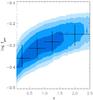 |
Fig. 8 Gas fraction distributions as a function of the redshift of model galaxies with
SSFR > tH(z)-1
and
M∗ > 1010 M⊙.
The filled contours correspond to equally spaced values of the density (per
Mpc3) of galaxies on a logarithmic scale: from 10-3 for the
lightest filled region to 10-2.1 for the darkest. The plotted value of
log fgas is the median value for sources in four
redshift bins: |
5. Conclusions
We have investigated the relative importance of the quiescent mode and burst mode of star formation in determining the SFR-M∗ relation and the evolution of the cosmic SFRD, predicted under the assumption that starburst events are triggered by galaxy encounters during their merging histories. The latter are described through Monte Carlo realizations and are connected to gas processes and star formation using an SAM of galaxy formation in a cosmological framework. The main results of this paper follow.
-
Hierarchical clustering models reproduce the slope and the scatter of the SFR-M∗ relation; however, they under-predict the normalization by a factor of 4–5 a z ≃ 2 (Daddi et al. 2007; Davé 2008; Fontanot et al. 2009; Damen et al. 2009; Santini et al. 2009; Lin et al. 2012). A possible theoretical explanation of this mismatch is that the amount of cold gas in galaxy disks predicted by these models at z ≃ 2 underestimates the real values. We derived the prediction for the evolution of the gas fraction distribution of star forming galaxies, as a prediction to be tested with future observations.
-
The tight correlation between SFR and M∗ of the galaxies on the main sequence is determined by the quiescent component of the star formation. Galaxies dominated by the star formation component induced by galaxy interactions populate the regions well above (major mergers) and below (minor mergers and fly-by events) the sequence.
-
The predicted SSFR distributions of star forming galaxies indicate that galaxies that are observationally classified as starburst on the basis of their distance from the main sequence (SSFRSB > 4 × SSFRMS) are indeed dominated by the burst component of the star formation. However, this criterion fails to select part of the burst-dominated star forming galaxies where galaxy interactions do not strongly boost the SFR.
-
Hierarchical clustering scenarios, connecting the properties of galaxies to their merging histories, naturally yield a fraction of starburst galaxies at z ~ 2 of ~1%, in agreement with the observational estimate (2% Rodighiero et al. 2011). This low fraction results because in this scenario, the statistics of merging events are dominated by minor episodes that do not produce SSFR above the observational threshold and to the low probability of finding a galaxy in a starburst phase due to the low value of the duration of the burst (t ≈ 107−108 yrs) compared with the typical time scale between galaxy encounters.
-
Quiescently star forming galaxies dominate the global SFRD at all redshifts. The contribution of the burst-dominated systems increases with redshift, rising from ≲5% at z ≲ 0.1 to ~20% at z ≥ 5. This behaviour is determined by the increase in the galaxy interaction rates and of the effectiveness of galaxy interaction in destabilizing the cold gas at high redshift. The fraction of the final (z = 0) galaxy stellar mass that is formed through the burst component of star formation is ~10% for 1010 M⊙ ≤ M∗ ≤ 1011.5 M⊙.
These findings do not imply that galaxy mergers/interactions play a lesser role in the formation of stars in galaxies. For each galaxy the star formation (both the quiescent and burst component) is indeed driven by the cooling rate of the hot gas and by the rate of refuelling of the cold gas, which in turn is intimately related to the galaxy merging histories.
We found that the interaction-driven model for starburst galaxies strictly predict the evolution and the mass dependence of the starburst contribution to the cosmic SFRD, which represent effective tools for testing this scenario with future observations of large and complete samples of star forming galaxies at z > 2. To reach this goal, a reliable observational diagnostic is also necessary that is able to distinguish between galaxies dominated by the quiescent and burst mode of star formation. The measure of the star formation efficiency and of the IR star formation compactness could represent eligible candidates for this purpose (Daddi et al. 2010; Genzel et al. 2010; Elbaz et al. 2011). The first is based on measurements of the mass and density of molecular gas at high redshift, and on the poor knowledge of the CO luminosity to H2 conversion factor. The technique of separating starbursts and quiescently star forming galaxies based on their IR star formation compactness seems to be promising, since ALMA will provide powerful tools for measuring the spatial distribution of star formation in distant galaxies at high angular resolution, making it possible to estimate the compactness of the star formation regions.
In this paper, we use the term quiescent to refer to star forming galaxies that are not in interaction. We do not mean non-star forming systems, as the term is used in some of the literature.
Acknowledgments
The authors thank Giulia Rodighiero for kindly providing the data plotted in Fig. 2, and the referee for helpful comments. This work was supported by ASI/INAF contracts I/024/05/0 and I/009/10/0 and PRIN INAF 2011.
References
- Barnes, J. E., & Hernquist, L. E. 1991, ApJ, 370, L65 [NASA ADS] [CrossRef] [Google Scholar]
- Barnes, J. E., & Hernquist, L. 1996, ApJ, 471, 115 [NASA ADS] [CrossRef] [Google Scholar]
- Baugh, C. M., Lacey, C. G., Frenk, C. S., et al. 2005, MNRAS, 356, 1191 [NASA ADS] [CrossRef] [Google Scholar]
- Blitz, L., & Rosolowsky, E. 2006, ApJ, 650, 933 [NASA ADS] [CrossRef] [Google Scholar]
- Bond, J. R., Cole, S., Efstathiou, G., & Kaiser, N. 1991, ApJ, 379, 440 [NASA ADS] [CrossRef] [Google Scholar]
- Bower, R. G., Benson, A. J., Malbon, R., et al. 2006, MNRAS, 370, 645 [NASA ADS] [CrossRef] [Google Scholar]
- Brinchmann, J., Charlot, S., White, S. D. M., et al. 2004, MNRAS, 351, 1151 [NASA ADS] [CrossRef] [Google Scholar]
- Cavaliere, A., & Vittorini, V. 2000, ApJ, 543, 599 [NASA ADS] [CrossRef] [Google Scholar]
- Daddi, E., Cimatti, A., Renzini, A., et al. 2004, ApJ, 617, 746 [NASA ADS] [CrossRef] [Google Scholar]
- Daddi, E., Dickinson, M., Morrison, G., et al. 2007, ApJ, 670, 156 [NASA ADS] [CrossRef] [Google Scholar]
- Daddi, E., Dannerbauer, H., Stern, D., et al. 2009, ApJ, 694, 1517 [Google Scholar]
- Daddi, E., Elbaz, D., Walter, F., et al. 2010, ApJ, 714, L118 [Google Scholar]
- Damen, M., Labbé, I., Franx, M., et al. 2009, ApJ, 690, 937 [NASA ADS] [CrossRef] [Google Scholar]
- Davé, R. 2008, MNRAS, 385, 147 [NASA ADS] [CrossRef] [Google Scholar]
- Dickinson, M., Papovich, C., Ferguson, H. C., & Budavári, T. 2003, ApJ, 587, 25 [NASA ADS] [CrossRef] [Google Scholar]
- Drory, N., & Alvarez, M. 2008, ApJ, 680, 41 [NASA ADS] [CrossRef] [Google Scholar]
- Drory, N., Bender, R., Feulner, G., et al. 2004, ApJ, 608, 742 [NASA ADS] [CrossRef] [Google Scholar]
- Durrell, P. R., Ciardullo, R., Feldmeier, J. J., Jacoby, G. H., & Sigurdsson, S. 2002, ApJ, 570, 119 [NASA ADS] [CrossRef] [Google Scholar]
- Eastman, J., Martini, P., Sivakoff, G., et al. 2007, ApJ, 664, L9 [NASA ADS] [CrossRef] [Google Scholar]
- Elbaz, D., Daddi, E., Le Borgne, D., et al. 2007, A&A, 468, 33 [NASA ADS] [CrossRef] [EDP Sciences] [Google Scholar]
- Elbaz, D., Dickinson, M., Hwang, H. S., et al. 2011, A&A, 533, A119 [NASA ADS] [CrossRef] [EDP Sciences] [Google Scholar]
- Engel, H., Tacconi, L. J., Davies, R. I., et al. 2010, ApJ, 724, 233 [NASA ADS] [CrossRef] [Google Scholar]
- Fanidakis, N., Baugh, C. M., Benson, A. J., et al. 2011, MNRAS, 410, 53 [NASA ADS] [CrossRef] [Google Scholar]
- Fanidakis, N., Baugh, C. M., Benson, A. J., et al. 2012, MNRAS, 419, 2797 [NASA ADS] [CrossRef] [Google Scholar]
- Fardal, M. A., Katz, N., Weinberg, D. H., & Davé, R. 2007, MNRAS, 379, 985 [NASA ADS] [CrossRef] [Google Scholar]
- Fontana, A., Donnarumma, I., Vanzella, E., et al. 2003, ApJ, 594, L9 [NASA ADS] [CrossRef] [Google Scholar]
- Fontana, A., Pozzetti, L., Donnarumma, I., et al. 2004, A&A, 424, 23 [NASA ADS] [CrossRef] [EDP Sciences] [Google Scholar]
- Fontana, A., Salimbeni, S., Grazian, A., et al. 2006, A&A, 459, 745 [NASA ADS] [CrossRef] [EDP Sciences] [Google Scholar]
- Fontana, A., Santini, P., Grazian, A., et al. 2009, A&A, 501, 15 [NASA ADS] [CrossRef] [EDP Sciences] [Google Scholar]
- Fontanot, F., De Lucia, G., Monaco, P., Somerville, R. S., & Santini, P. 2009, MNRAS, 397, 1776 [NASA ADS] [CrossRef] [Google Scholar]
- Fu, J., Kauffmann, G., Li, C., & Guo, Q. 2012, MNRAS, 424, 2701 [NASA ADS] [CrossRef] [Google Scholar]
- Genzel, R., Tacconi, L. J., Gracia-Carpio, J., et al. 2010, MNRAS, 407, 2091 [NASA ADS] [CrossRef] [Google Scholar]
- Glazebrook, K., Abraham, R. G., McCarthy, P. J., et al. 2004, Nature, 430, 181 [NASA ADS] [CrossRef] [Google Scholar]
- González, V., Labbé, I., Bouwens, R. J., et al. 2011, ApJ, 735, L34 [NASA ADS] [CrossRef] [Google Scholar]
- Guo, Q., White, S., Boylan-Kolchin, M., et al. 2011, MNRAS, 413, 101 [NASA ADS] [CrossRef] [Google Scholar]
- Henriques, B. M. B., & Thomas, P. A. 2010, MNRAS, 403, 768 [NASA ADS] [CrossRef] [Google Scholar]
- Hernquist, L. 1989, Nature, 340, 687 [NASA ADS] [CrossRef] [Google Scholar]
- Hirschmann, M., Somerville, R. S., Naab, T., & Burkert, A. 2012, MNRAS, 426, 237 [NASA ADS] [CrossRef] [Google Scholar]
- Hopkins, A. M., & Beacom, J. F. 2006, ApJ, 651, 142 [NASA ADS] [CrossRef] [MathSciNet] [Google Scholar]
- Hopkins, P. F., Younger, J. D., Hayward, C. C., Narayanan, D., & Hernquist, L. 2010, MNRAS, 402, 1693 [NASA ADS] [CrossRef] [Google Scholar]
- Kennicutt, Jr., R. C. 1998, ApJ, 498, 541 [NASA ADS] [CrossRef] [Google Scholar]
- Krumholz, M. R., McKee, C. F., & Tumlinson, J. 2009, ApJ, 699, 850 [NASA ADS] [CrossRef] [Google Scholar]
- Lacey, C., & Cole, S. 1993, MNRAS, 262, 627 [NASA ADS] [CrossRef] [Google Scholar]
- Lagos, C. D. P., Baugh, C. M., Lacey, C. G., et al. 2011a, MNRAS, 418, 1649 [NASA ADS] [CrossRef] [Google Scholar]
- Lagos, C. D. P., Lacey, C. G., Baugh, C. M., Bower, R. G., & Benson, A. J. 2011b, MNRAS, 416, 1566 [NASA ADS] [CrossRef] [Google Scholar]
- Lamastra, A., Menci, N., Maiolino, R., Fiore, F., & Merloni, A. 2010, MNRAS, 405, 29 [NASA ADS] [Google Scholar]
- Lin, L., Dickinson, M., Jian, H.-Y., et al. 2012, ApJ, 756, 71 [NASA ADS] [CrossRef] [Google Scholar]
- Marchesini, D., van Dokkum, P. G., Förster Schreiber, N. M., et al. 2009, ApJ, 701, 1765 [NASA ADS] [CrossRef] [Google Scholar]
- Martini, P., Sivakoff, G. R., & Mulchaey, J. S. 2009, ApJ, 701, 66 [NASA ADS] [CrossRef] [Google Scholar]
- Menci, N., Cavaliere, A., Fontana, A., et al. 2004, ApJ, 604, 12 [NASA ADS] [CrossRef] [Google Scholar]
- Menci, N., Fontana, A., Giallongo, E., & Salimbeni, S. 2005, ApJ, 632, 49 [NASA ADS] [CrossRef] [Google Scholar]
- Menci, N., Fontana, A., Giallongo, E., Grazian, A., & Salimbeni, S. 2006, ApJ, 647, 753 [NASA ADS] [CrossRef] [Google Scholar]
- Menci, N., Fiore, F., Puccetti, S., & Cavaliere, A. 2008, ApJ, 686, 219 [NASA ADS] [CrossRef] [Google Scholar]
- Mihos, J. C., & Hernquist, L. 1994, ApJ, 431, L9 [NASA ADS] [CrossRef] [Google Scholar]
- Mihos, J. C., & Hernquist, L. 1996, ApJ, 464, 641 [NASA ADS] [CrossRef] [Google Scholar]
- Mo, H. J., Mao, S., & White, S. D. M. 1998, MNRAS, 295, 319 [Google Scholar]
- Moore, B., Katz, N., Lake, G., Dressler, A., & Oemler, A. 1996, Nature, 379, 613 [NASA ADS] [CrossRef] [Google Scholar]
- Noeske, K. G., Weiner, B. J., Faber, S. M., et al. 2007, ApJ, 660, L43 [Google Scholar]
- Papovich, C., Dickinson, M., & Ferguson, H. C. 2001, ApJ, 559, 620 [NASA ADS] [CrossRef] [Google Scholar]
- Papovich, C., Moustakas, L. A., Dickinson, M., et al. 2006, ApJ, 640, 92 [NASA ADS] [CrossRef] [Google Scholar]
- Pilbratt, G. L., Riedinger, J. R., Passvogel, T., et al. 2010, A&A, 518, L1 [CrossRef] [EDP Sciences] [Google Scholar]
- Pozzetti, L., Bolzonella, M., Lamareille, F., et al. 2007, A&A, 474, 443 [NASA ADS] [CrossRef] [EDP Sciences] [Google Scholar]
- Rodighiero, G., Daddi, E., Baronchelli, I., et al. 2011, ApJ, 739, L40 [NASA ADS] [CrossRef] [Google Scholar]
- Rudnick, G., Labbé, I., Förster Schreiber, N. M., et al. 2006, ApJ, 650, 624 [NASA ADS] [CrossRef] [Google Scholar]
- Salim, S., Rich, R. M., Charlot, S., et al. 2007, ApJS, 173, 267 [NASA ADS] [CrossRef] [Google Scholar]
- Sanders, D. B., & Mirabel, I. F. 1996, ARA&A, 34, 749 [NASA ADS] [CrossRef] [Google Scholar]
- Santini, P., Fontana, A., Grazian, A., et al. 2009, A&A, 504, 751 [NASA ADS] [CrossRef] [EDP Sciences] [Google Scholar]
- Santini, P., Fontana, A., Grazian, A., et al. 2012, A&A, 538, A33 [NASA ADS] [CrossRef] [EDP Sciences] [Google Scholar]
- Saslaw, W. C. 1985, Gravitational physics of stellar and galactic systems (CUP) [Google Scholar]
- Shapley, A. E., Steidel, C. C., Adelberger, K. L., et al. 2001, ApJ, 562, 95 [NASA ADS] [CrossRef] [Google Scholar]
- Shapley, A. E., Steidel, C. C., Erb, D. K., et al. 2005, ApJ, 626, 698 [NASA ADS] [CrossRef] [Google Scholar]
- Somerville, R. S., Primack, J. R., & Faber, S. M. 2001, MNRAS, 320, 504 [NASA ADS] [CrossRef] [Google Scholar]
- Spergel, D. N., Bean, R., Doré, O., et al. 2007, ApJS, 170, 377 [NASA ADS] [CrossRef] [Google Scholar]
- Stark, D. P., Ellis, R. S., Bunker, A., et al. 2009, ApJ, 697, 1493 [NASA ADS] [CrossRef] [Google Scholar]
- Tacconi, L. J., Genzel, R., Smail, I., et al. 2008, ApJ, 680, 246 [NASA ADS] [CrossRef] [PubMed] [Google Scholar]
- White, S. D. M., & Rees, M. J. 1978, MNRAS, 183, 341 [NASA ADS] [CrossRef] [Google Scholar]
- Wilkins, S. M., Trentham, N., & Hopkins, A. M. 2008, MNRAS, 385, 687 [NASA ADS] [CrossRef] [Google Scholar]
- Yan, H., Dickinson, M., Giavalisco, M., et al. 2006, ApJ, 651, 24 [NASA ADS] [CrossRef] [Google Scholar]
- Zwicky, F. 1951, PASP, 63, 61 [Google Scholar]
All Figures
|
Fig. 1 SFHs drawn from the Monte Carlo realizations of galaxies, which, at z = 0, have masses of M∗ ≃ 1010 M⊙ (left) and M∗ ≃ 1012 M⊙ (right). The SFHs are obtained by summing over all the progenitors that have merged to form galaxies of the selected final mass. The quiescent star formation is represented by the smooth component of the SFHs, the burst component by the impulsive one. The duration of the SFR-excess phase due to the interactions is represented by the width of the peak of the SFHs. |
| In the text | |
|
Fig. 2 Left: SFR-M∗ relation at 1.5 < z < 2.5. The five filled contours correspond to equally spaced values of the density (per Mpc3) of model galaxies in logarithmic scale: from 10-6 for the lightest filled region to 10-2 for the darkest. Green squares: Herschel-PACS- selected galaxies, black circles: BzK galaxies, from the Rodighiero et al. (2011) sample; blue triangles: GOODS-MUSIC catalogue from the Santini et al. (2009) sample. The dashed and long-dashed lines indicate the best-fit of the galaxy main sequence obtained by Rodighiero et al. (2011) and Santini et al. (2009) respectively, while the solid line shows the spline fit to the peaks of the SFR distributions of model galaxies as a function of stellar mass. Right: SSFR as a function of M∗. Colour code, symbols, and solid line as in the left panel. The dashed and thin solid lines respectively indicate the SSFR > SSFRMS − 2σ and the SSFR > tH(z)-1 limits of the galaxy samples used in the analysis of Sect. 3.2. |
| In the text | |
|
Fig. 3 Predicted SFR-M∗ relation at 1.5 < z < 2.5 obtained by selecting from the model galaxies dominated by the quiescent (left) and burst (right) mode of star formation. Contours and solid line as in Fig. 2. |
| In the text | |
|
Fig. 4 SSFR distributions of model galaxies, at 1.5 < z < 2.5, in four mass bins. The blue histograms refer to galaxies dominated by the quiescent mode of star formation, the red histograms to galaxies dominated by the burst mode of star formation, and the green histograms to galaxies with an interaction-driven star formation component. The solid vertical lines show the position of the main sequence, while the vertical dotted lines show the SSFR threshold used to identify starburst galaxies: SSFRSB > 4 × SSFRMS. The solid distributions are obtained by selecting galaxies with SSFR > tH(z)-1, while dashed distributions are obtained selecting galaxies with SSFR > SSFRMS − 0.6 dex. |
| In the text | |
|
Fig. 5 Left: fraction of starburst (shaded region), burst-dominated (hatched region), and interacting (triangles) galaxies as function of the stellar mass at 1.5 < z < 2.5. Right: contribution to the cosmic SFRD of the same classes of star forming galaxies. The lines indicate the model predictions when adopting the SSFR > tH(z)-1 (solid lines) and the SSFR > SSFRMS-2σ (dashed lines) criterion to define the global sample of star forming galaxies. The data points indicate the results obtained by Rodighiero et al. (2011) for starburst galaxies (SSFR > 4 × SSFRMS). |
| In the text | |
|
Fig. 6 Contribution to the cosmic SFRD of galaxies with SFR ≥ 1.4 × 10⁻⁶ M⊙/yr (corresponding to UV luminosity LUV ≳ 1015 W Hz−1 when adopting the calibration given in Kennicutt 1998) as a function of redshift (solid line). Dashed line indicates the contribution of galaxies dominated by the quiescent mode of star formation, while dotted line indicates the contribution of galaxies dominated by the burst mode of star formation. |
| In the text | |
|
Fig. 7 Predicted average values of the ratio Mburst(z)/M∗(z) as a function of redshift and galaxy stellar mass. The four filled contours correspond to equally spaced values of the ratio Mburst(z)/M∗(z): from 0.05 for the lightest filled region to 0.2 for the darkest. The lines illustrate the growth histories of a typical galaxy with final mass: M∗(z = 0) = 1012 M⊙ (red), M∗(z = 0) = 1011 M⊙ (blue), and M∗(z = 0) = 1010 M⊙ (purple). |
| In the text | |
|
Fig. 8 Gas fraction distributions as a function of the redshift of model galaxies with
SSFR > tH(z)-1
and
M∗ > 1010 M⊙.
The filled contours correspond to equally spaced values of the density (per
Mpc3) of galaxies on a logarithmic scale: from 10-3 for the
lightest filled region to 10-2.1 for the darkest. The plotted value of
log fgas is the median value for sources in four
redshift bins: |
| In the text | |
Current usage metrics show cumulative count of Article Views (full-text article views including HTML views, PDF and ePub downloads, according to the available data) and Abstracts Views on Vision4Press platform.
Data correspond to usage on the plateform after 2015. The current usage metrics is available 48-96 hours after online publication and is updated daily on week days.
Initial download of the metrics may take a while.