| Issue |
A&A
Volume 551, March 2013
|
|
|---|---|---|
| Article Number | A101 | |
| Number of page(s) | 17 | |
| Section | Planets and planetary systems | |
| DOI | https://doi.org/10.1051/0004-6361/201219917 | |
| Published online | 01 March 2013 | |
Using the Sun to estimate Earth-like planets detection capabilities
IV. Correcting for the convective component
UJF-Grenoble 1/CNRS-INSU, Institut de Planétologie et d’Astrophysique de Grenoble (IPAG) UMR 5274, 38041 Grenoble, France
e-mail: This email address is being protected from spambots. You need JavaScript enabled to view it.
Received: 29 June 2012
Accepted: 12 December 2012
Abstract
Context. Radial velocity (RV) time series are strongly impacted by the presence of stellar activity. In a series of papers, we have reconstructed solar RV variations over a full solar cycle from observed solar structures (spots and plages) and studied their impact on the detectability of an Earth-mass planet in the habitable zone of the Sun as seen edge-on from a neighbour star in several typical cases. We found that the convective contribution dominates the RV times series.
Aims. The objective of this paper is twofold: to determine detection limits on a Sun-like star seen edge-on with different levels of convection and to estimate the performance of the activity correction using a Ca index.
Methods. We apply two methods to compute the detection limits: a correlation-based method and a local power analysis method, which both take into account the temporal structure of the observations. Furthermore, we test two methods using a Ca index to correct for the convective contribution to the RV: a sinusoidal fit to the Ca variations and a linear fit to the RV-Ca relation. In both cases, we use observed Ca and reconstructed Ca to study the various effects and limitations of our estimations.
Results. We confirm that an excellent sampling is necessary to have detection limits below 1 MEarth (e.g. 0.2−0.3 MEarth) when there is no convection and a low RV noise. With convection, the detection limit is always above 7 MEarth. The two correction methods perform similarly when the Ca time series are noisy, leading to a significant improvement (down to a few MEarth), which is above the 1 MEarth limit. With a very good Ca noise (signal to noise ratio, S/N, around 130), the sinusoidal method does not get significantly better because it is dominated by the fact that the solar cycle is not sinusoidal, but the RV-Ca method can reach the 1 MEarth for an excellent Ca noise level.
Conclusions. For Sun-like conditions and under the simplifying assumptions considered, we first conclude that the detection limit of a few MEarth planet can be reached providing good sampling and Ca noise. The detection of a 1 MEarth may be possible, but only with an excellent temporal sampling and an excellent Ca index noise level: we estimate that a probability larger than 50% to detect a 1 MEarth at 1.2 AU requires more than 1000 well-sampled observations and a Ca S/N larger than 130.
Key words: techniques: radial velocities / Sun: activity / Sun: surface magnetism / stars: early-type
© ESO, 2013
1. Introduction
The radial velocity (RV) technique has been a very powerful method to detect exoplanets since 1995. Thanks to their increased precision and stability, RV instruments allow us to detect lower mass planets and become more sensitive to stellar-induced variability, such as magnetic activity and pulsations. The influence of magnetic structures such as spots is quite well known, and has been studied by several groups (for example, Saar & Donahue 1997; Hatzes 2002; Desort et al. 2007; Lagrange et al. 2010). We have reconstructed the RV variations that would be produced by activity over a solar cycle, first by spots only (Lagrange et al. 2010, hereafter Paper I) and then by taking into account plages and the attenuation of the convective blueshift by the magnetic field (Meunier et al. 2010a, hereafter Paper II). Our simulations are based on observed solar structures for a seen edge-on Sun and are therefore representative of solar-type stars with a similar level of activity. We found that the role of convection is dominant and the typical amplitudes of the RV signal (of the order of 8 m/s over a cycle) are compatible with stellar observations (Isaacson & Fischer 2010; Lovis et al. 2011; Dumusque et al. 2011).
In Paper II, the impact of activity on the detectability was studied by adding planets at the proper periods in a few simple cases and looking at the periodogram. To get a more quantitative estimation of the impact, it is necessary to compute detection limits that take into account the impact of the phase of the planet.
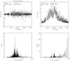 |
Fig. 1 Upper panels: reconstructed series for spots+plages RVsppl (left) and all components including convection RVtot (right). Set 3 and Set 4 are indicated by horizontal arrows. Set 1 and Set 2 cover the whole range. Lower panels: corresponding periodograms. The periodograms are in the same arbitrary units. |
We found out that the convection was dominating the signal and was the main limitation to planet detection. It is therefore important to find a way to estimate stellar activity and to efficiently correct for it. A possible approach is to use the variations in Ca index and to look for correlations with the RV signal. This has been done by Boisse et al. (2011), for example, in the case of a simple stellar activity signal (one spot). It is important to remember, however, that the Ca index is related to plages only and that when the activity pattern is complex, we do not expect in general a correlation between the Ca index and the RV signal. This lack of correlation is due to spot and plages (when considering the photometric contribution to the RV signal), as shown in Papers I and II. The contribution of the convection to the RV signal, however, should be strongly correlated with the Ca index, as both are directly related to the filling factor of plages. If the convection is dominant over spots, we expect the Ca index to be a good indicator. Dumusque et al. (2011) have used the Ca index to correct for the activity contribution of four stars (stellar types K and F) with a solar-like magnetic cycle, which allowed them to detect planets with masses between 0.22 and 2 MJup. This shows that it is possible to correct part of the convection signal using the Ca index, but to a yet undetermined precision. An important issue is whether it is possible to reach the 1 MEarth detection limit level in the habitable zone for a solar-type star with an activity level and pattern similar to the Sun.
We note that the use of the Ca index is not the only way to deal with this issue. Aigrain et al. (2012) have implemented a method to derive activity-induced RV variation from photometric time series and applied it to stellar observations and to the solar-reconstructed RV used in this paper. Photometric variations have also been fitted in order to extract information about the spots and plages (e.g. Lanza et al. 2007). These methods, however, do not take into account the convection contribution.
The objectives of this paper are therefore twofold: i) to determine the detection limits on reconstructed solar RV for different levels of convection; ii) to propose and test a method to correct for the convective component. In Sect. 2, we therefore compute the detection limits on the RV time series for various temporal samplings and RV noise conditions. We also evaluate the impact of the amplitude of the convective component on the detection limits. While we focus our study on light planets at 1.2 AU, we also study the impact of the distance on the detection limits. In Sect. 3, we describe the Ca emission activity index (observed and model) that will be used to correct for the convective contribution. In Sect. 4, we evaluate two methods to perform this correction, and in Sect. 5 we study their limitations. We illustrate our results for a 1 MEarth planet in Sect. 6 and discuss them in Sect. 7.
2. Detection limits on reconstructed radial velocities
2.1. Time series and method
In this section, we compute the detection limits for the time series presented in Paper II and shown in Fig. 1, hereafter RVsppl (spots and plages only, without convection) and RVtot (all components, including the convection component RVconv). We used spots and plages observed daily over one cycle to build solar maps and derive spectra. The RV time series result from the sum of three components computed on the spectra: the RV variations due to the spot temperature contrast; the RV variations due to the plage temperature contrast; the convective component due to the attenuation of the convective blueshift in the presence of magnetic fields present in plages. The sum of the two first components corresponds to RVsppl, while RVtot corresponds to all components. We analyse the influence of the sampling and of the noise associated with these RV data on the detection limits.
2.1.1. Temporal samplings
The temporal samplings are the following. On the original time series (covering solar cycle 23, with a temporal cadence close to one day), we first apply a mask eliminating four months per year to simulate the fact that a star is not observable throuhgout the year. This should naturally introduce a one-year periodicity in the time series. In the resulting time series, we consider four temporal samplings:
-
All points (hereafter one-day sampling),
-
1 point every 4 days,
-
1 point every 8 days,
-
1 point every 20 days.
To avoid introducing the sampling periodicity, in the last three considered cases, we add a time shift to the sampling between −2 days and +2 days (randomly) to each observing time. Because there are a few gaps in the original time series, these gaps are still present in the final times series. What is mostly tested here is the number of observation, for a given length of the time series. The typical number of points for each sampling is shown in Table 1: they range from 2377 for the best sampling to 131 for the worse. These different samplings applied to the full time series correspond in the following to Set 1.
In addition, we study a smaller data set, hereafter Set 2, for which we have a measured solar Ca index1 (978 points, covering the full cycle and thus exhibiting the full range of activity levels). We apply to this data the same sampling selection as above, i.e. we consider all points or 1 point every 4, 8 or 20 days on the time series. We note that because Set 2 covers the same length as Set 1 but with fewer points, the actual sampling is sparser: all points of Set 2 after the four-month gaps represent about 3.2 times fewer points for the same duration. We therefore multiply the sampling by 3.2 for Set 2 to correspond to the sparser effective sampling.
Typical number of observations.
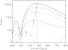 |
Fig. 2 Periodograms (zoom on the wide peaks) of the RV variations produced by a 100 (respectively 75, 50, 25, 5 from top to bottom) MEarth planet at a phase of zero and period of 480.1 days, for Set 3, solid line (respectively dashed, dotted, dot-dashed, dot-dot-dot-dashed). The vertical line indicates the theoretical position of the peak. The arrows indicate the position of the planet peak for each planet mass. |
Finally, to study the impact of the activity level and of shorter time series, we define two other samples, each covering three years and corresponding to different activity levels: Set 3 corresponds to the three first years of the cycle (low activity level) and Set 4 corresponds to three years during the maximum of activity. The typical number of points for all samples is shown in Table 1.
2.1.2. RV noise
As in Paper II, we add noise to the RV data with levels as expected from future instruments (VLT/Espresso, E-ELT/Codex). We therefore consider four RV noise levels in the following: no noise, 1 cm/s, 5 cm/s, and 10 cm/s. Unless stated precisely, we compute detection limits for a planet at 1.2 AU, i.e. with a period of 480.1 days, to avoid a planet peak at one year that might be in conflict with observation peaks.
2.1.3. Detection limits
In this paper we use two methods to compute the detection limits. They are described in more detail in Meunier et al. (2012, hereafter Paper III):
-
the correlation-based method (based on the correlation betweenthe stellar signal added to the planet signal with the planet signalalone),
-
the local power amplitude (LPA) method, based on the comparison of the power that is due to the planet and localised around the planet period, with the power in the RV series without the planet.
As in Paper III, the detection limits are computed assuming circular orbits.
In Paper III, we also used two other methods: the root mean squared (rms) method (based on the comparison of the amplitude planet signal and the rms of the observed signal), and the peak method (based on the comparison of the amplitude of the peak at the planet period with the amplitude of other peaks in the periodogram). The rms method usually gives the largest value because it does not take into account the temporal structure of the signal and is dominated by the rotation modulation. The peak method, which was shown to be the least robust in Paper III, also gives larger detection limits. Furthermore, even for a massive planet producing a large peak, the period of the peak can be significantly different from the planet period of 480.1 days. This is mostly seen for Set 3 and Set 4 and for RVtot. An example is shown in Fig. 2: we observe a shift of the peak period towards lower (in that example) periods as the planet mass decreases, even if the peak remains large. This is probably due to a combination of the temporal sampling (which creates some strong peaks at various periods in the periodograms) and the power structure of the RV signal. This is another illustration of the fact that this method is less robust. In the following, we only consider the results obtained with the correlation-based method and the LPA one, as these give the best detection limits and were shown to be more robust.
2.1.4. Parameters
In Sect. 4, we evaluate the possibility to correct for the contribution of the convection to the RV signal by using measured activity indexes in the calcium line. The detection limit after correction will be computed and compared to those of the present section to estimate the performances of the various methods to correct for the convection signal. To understand better the results and to characterise the corrected time series, it is useful to define three parameters:
-
the rms of the corrected signal,
-
the total power in the periodogram for periods between 50 and 1000 days,
-
the correlation between the RV time series after correction and the spot+plage signal RVsppl time series.
The comparison of these parameters after correction will show the amount of improvement with respect to the RV signal with convection RVtot and how the detection limits after correction are close to the signal without convection RVsppl.
2.2. Results for a planet at 1.2 AU
2.2.1. Case without convection
Figure 3 shows the detection limits versus sampling for various noise conditions when considering the reconstructed RVsppl for spots and plages only (i.e. without taking into account the convection contribution) for Set 1. Our purpose is to test the impact of the RV noise on the results. It appears that the variations in detection limits are dominated by the sampling and the RV noise, at least up to a level of 10 cm/s, is negligible, as already noted in Paper II. This is the case for the two methods used to compute the detection limits for RVtot and the other data set (Sets 2, 3, 4).
For the RVsppl signal, the two methods give detection limits that are close to each other when the sampling is good. The detection limits for all data sets are shown in Fig. 4 (two upper rows). For an excellent temporal sampling, the detection limits are below or around 1 MEarth and remain good with sparser sampling, although closer to the 2 MEarth regime or above.
The three parameters defined in Sect. 2.1.4 are shown in Fig. 5 (green symbols). The rms RV is typically 0.3 m/s, the power in the range 30−60. The correlation is, as expected, 1 in this case. These values will serve as a reference when evaluating the performances of the correction method in Sect. 4.
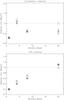 |
Fig. 3 Detection limits versus sampling for RVsppl (i.e. no convection), Set 1, and a planet at 1.2 AU. Different RV noise levels are considered: no noise (stars), 1 cm/s (diamonds), 5 cm/s (triangle), and 10 cm/s (square). Each panel corresponds to a detection limit method. |
2.2.2. Case with convection
Figure 4 (last two rows) shows the detection limits for RVtot and all samples for no noise on the RV signals. In that case, even in the best conditions in terms of sampling (i.e. close to 1 point per day over a cycle) and noise, the detection limit is significantly above 1 MEarth: for Set 1, it is about 7 MEarth (i.e. in the Super-Earth regime) with the most optimistic method (correlation-based method), and the LPA method provides detection limits above 15 MEarth at best. The detection limits are worse as the sampling is degraded, especially for 1 observation every 20 days. They are also significantly degraded for the other sets and are above 10 MEarth for Set 2 and 3 and above 16 MEarth for Set 4.
The three parameters (rms RV, total power, and correlation with RVsppl) are shown in Fig. 5 (red symbols). The rms RV is typically around 2.5 m/s for Set 1 and Set 2, which are covering the full cycle. They are lower for the other data sets that span a smaller time range, i.e. showing a smaller long-term variation. The power is in the range 103−104, i.e. between 1 and 2.5 order of magnitude above the RVsppl level. The correlation between RVsppl and RVtot is small, between 0 and 0.2.
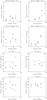 |
Fig. 4 Two first rows: detection limits versus sampling for the spots+plages RV signal for Sets 1 to 4, no RV noise, for the correlation-based method (stars, orange), and the LPA method (squares, blue). Two last rows: same for the total RV signal. |
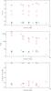 |
Fig. 5 Upper panel: rms of the RV signal versus the sampling for zero RV noise, for the spots+plages RV signal (green), and for the total RV signal (red) for Set 1 (stars), Set 2 (diamonds), Set 3 (triangle), and Set 4 (squares). Middle panel: same for the total power computed from the periodogram. Lower panel: same for the correlation with the spots+plages RV signal corresponding to the same sampling. |
2.2.3. Impact of the presence of a planet
The detection limits are impacted by the presence of a planet because the detection limit computations are based on the assumption that there is no planet: the detection limits are therefore always larger than the mass of such a planet if it is present in the RV signal. For example, a 5 MEarth planet will lead to a peak of amplitude A and the detection limit methods will search for peaks larger than A. Figure 6 shows the periodograms for a 1 MEarth alone for Set 1 and best sampling, to be compared with the periodograms when the activity signal is added (without or with convection). This shows that the detection limit below 1 MEarth for the case without convection is realistic as the planet peak is very significant, while the planet peak is much below the activity power when convection is present.
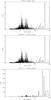 |
Fig. 6 Upper panel: periodogram of a 1 MEarth at 1.2 AU with the Set 1 sampling (all days). The vertical dotted line indicates the position of the planet peak. Middle panel: same for the RVsppl added to the signal of this planet. Lower panel: same for the RVtot added to the signal of this planet. Power is in arbitrary unit but on the same scale on all plots. |
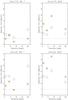 |
Fig. 7 Upper left panel: detection limits versus sampling for a modified RVtot corresponding to a convection contribution ten times smaller than the solar one for Set 1. Detection limits are computed using the correlation-based method (stars, orange), and the LPA method (squares, blue). There is no noise level on the RV signal. Upper right panel: same for Set 3. Lower panels: same for a convection contribution five times smaller than the solar one. |
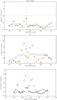 |
Fig. 8 Upper panel: detection limits versus planet period for RVsppl (Set 1, no RV noise, daily sampling). Detection limits are computed using the correlation-based method (stars, orange), and the LPA method (squares, blue). Middle panel: same for RVtot. Lower threshold: correlation threshold for RVsppl (stars) and RVtot (diamonds). The vertical dashed lines indicate the one-year period position. |
2.2.4. Results for different convection levels
To get an idea of the impact of the convection level on the detection limits, we compute the same detection limits as before but after changing the level of convection in RVtot. The results are shown in Fig. 7 for selected examples and no RV noise, to be compared with Fig. 4. For Set 1, for example, they are in the range 1−2 MEarth for a convection divided by 10 and in the range 2−7 MEarth for a convection divided by 5, instead of 6−23 MEarth, when full convection is taken into account. We find that, as estimated in Paper II from periodogram analysis in a few cases, a very low level of convection (one order of magnitude weaker than in the Sun) is necessary to reach the Earth-mass regime: with levels of convection ten times lower, the detection limits obtained for an excellent sampling, although larger than the RVsppl detection limits obtained in Sect. 2.2.1, are close to one Earth mass. With levels of convection five times lower, detection limits of a few Earth masses can be reached, i.e. moderate levels of convection may make it possible to reach the Super-Earth mass regime. These results also give an idea of the amplitude of the correction of the convective component that needs to be reached under a perfect case (no RV noise). When adding the RV noise, the results are similar to that of Fig. 3, i.e. the impact is very small (no difference or of the order of the mass step).
2.3. Results for planets at different periods
Here we compute the detection limits in the same conditions for other periods between 200 and 600 days. The results are shown in Fig. 8 for Set 1 and all points considered. With no convection (upper panel), the detection limits are similar to the one at 1.2 AU and are all below 1 MEarth. With convection (lower panel), they are all above 1 MEarth. The high values in the range 320−440 days, especially for RVtot, are likely due to the temporal sampling including a four-month gap every year, this introduces some power around 365 days. The correlation-based detection limits are noisier than the LPA detection limits, because the correlation threshold is less stable (and more dependent on the temporal sampling of the observation, as described in Paper III), which directly impacts the detection limits.
3. The Ca time series
In the next section we test two methods using the calcium activity index to correct the convective component, as both quantities are strongly correlated (Paper II). The reason for using the calcium activity index is that, on the one hand, the RV amplitude induced by the convection is proportional to the surface covered by plages and, on the other hand, the calcium emission is also proportional to the surface covered by plages2. In this section we describe the Ca time series we are using.
3.1. Observed Ca time series
We use the measured solar calcium emission index (Sacramento Peak Observatory), hereafter Ca, measured during the same cycle. It is available on a smaller number of days than for the complete data set (978 points over the considered cycle instead of 3586 points for Set 1, without the four-month gaps). When using this time series, we will compare our results with those presented in the previous section for Set 2.
Using a measured Ca index has the advantages of giving realistic variations of the chromospheric emission. The noise level on the Sacramento Peak index is estimated to be about 0.6%3, corresponding to a signal-to-noise ratio (S/N) of about 166.
3.2. Building reconstructed Ca time series
Due to the limited number of Ca measurements, we decided to test the performance of the Ca correction using reconstructed Ca, which would allow the full time series to be covered. As already mentioned, there is a strong correlation between the filling factor of plages and network and the total RV when the latter is dominated by the convection (i.e. a strong attenuation of the convection in plages, ΔV, is necessary to have this correlation) and there is also a strong correlation between this filling factor and the Ca emission. Because both Ca and RV (due to convection) are correlated with the filling factor (hereafter ff), we are able to build an artificial Ca time series to test our correction method on longer time series. This is possible because we know ff, which we would not know in the case of stellar observations: the ff is used here to build Ca times series in order to test the method, but is not used to perform the correction. As a consequence, this represents an ideal case, because the dispersion due to temperature and magnetic field variations between different localisations in plages is not taken into account (see Sect. 5.2).
The first step is to use the correlation between ff and measured Ca on 978 points to build a law that relates ff and Ca. In our case, this law is Ca = 0.0879+2.63 10-7 ff, resulting from a linear fit between the measured Ca (Sect. 3.1) and the corresponding reconstructed ff. This basic law is then used to build Ca on the whole sample (because the simulation provides ff). In the following, we consider four noise levels:
-
no noise (hereafter σ0).
-
a noise level similar to the most optimistic conditions determined by Lovis et al. (2011), i.e. 7 × 10⁻⁴ (hereafter σhigh) and corresponding to the smallest dispersion observed in their sample. It corresponds to an average S/N on Ca of about 130. This is only slightly below the S/N for solar observations (166), for which many more photons are available than for any other stars, and is therefore very optimistic.
-
a noise level of 1.9 × 10⁻³ (hereafter σmed). It corresponds to an average S/N of about 50.
-
a noise level that would be obtained for the faintest stars (9.4 × 10⁻³, hereafter σlow), which corresponds to an average S/N of 10.
When adding the noise (i.e. all cases except the first one), we perform ten realisations of the noise4. An example of the Ca time series for each noise level is shown in Fig. 9.
4. Correction of the convective component
In this section, we evaluate two methods to correct for the contribution of convection to the RV variations. We first study the possibility to use a sinusoidal fit on the Ca II index to correct for the RV variations from the convection component. In the second approach, we use the correlation between Ca II index and the RV to derive a correction. In both cases we will use either the observed Ca or the reconstructed Ca described in Sect. 3.
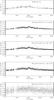 |
Fig. 9 From top to bottom: observed Ca emission index (Sacramento peak, upper panel) and reconstructed Ca index with various noise levels (see Sect. 3.2), for all available data points. |
4.1. Correction using sinusoidal Ca fitting
4.1.1. The method
In this section, we fit the Ca variations and then use the derived period to fit a sinusoidal function on the observed RV (the period being fixed and equal to the Ca one). Such an approach was adopted for different stars observed over long periods of time (activity cycles) by Dumusque et al. (2011); Lovis et al. (2011). We use this approach with reconstructed Ca with no noise and with the observed Ca.
4.1.2. The results
The results for the best sampling of Set 1 and Set 2 are shown in Table 2 (for the reconstructed Ca, no Ca noise). An example of the corrected RV obtained for the Sun is shown in Fig. 10. The corresponding detection limits are shown in Fig. 11.
For Set 2 (lower panel of Fig. 11), the detection limits are in the range 2.5−5.8 MEarth, depending on the method for the best sampling. They are above 10 MEarth for the worst samplings. When applied to the observed Ca, the detection limits are similar to those obtained with the reconstructed Ca when comparing the same set (Set 2). The Ca measurements are made on a limited number of days, but this does not impact the sinusoidal fit as the data cover the whole cycle.
For Set 1, with the best sampling, the correlation-based detection limit is about 2 MEarth, and it is about 4.5 MEarth for the LPA method. For Set 1 and 1 point every 20 days, it is in the range 7−8 MEarth. This correction method therefore allows the detection limits to be significantly (by a factor ~4) improved (as in Dumusque et al. 2011), but does not allow the 1 MEarth range and the RVsppl detection limit (first line in the table) to be reached.
These detection limits can be explained by the variations of the parameters (defined in Sect. 2.1.4): for Set 1 for example, the rms RV remains large after correction (in the range 1.3−1.5 m/s), as the power is closer to the value before correction (corresponding to RVtot) than to the RVsppl level (our objective if the correction was perfect), while the correlation with RVsppl is not improved at all. Furthermore, the rms RV after correction for observed Ca and reconstructed Ca (around 1.3 m/s for Set 2) is also almost the same, as are the periodograms: they are not dominated by the Ca noise (present in observed Ca but not in the reconstructed Ca), but by the large residuals due to the sinusoidal fit. This is mostly due to the fact that the solar cycle variations are not sinusoidal. They are not only asymmetric (the rising phase is faster than the decreasing phase), but they also present some significant variations for time scales of a year or a few years. These are of large amplitude and are not corrected here. Therefore, we conclude that this method is not adequate to perform a precise correction of the convective component, even with no noise.
The Ca noise therefore has a strong impact on the detection limits. Furthermore, computations made for reconstructed Ca with a given noise level show a dispersion in detection limit (see Table 2), and this effect is stronger for low S/N. The results are therefore sensitive to the realisation of the Ca noise. This is studied in more detail in Sect. 5.1.
Detection limits for the best sampling of Set 1 and Set 2 for selected conditions and a planet at 1.2 AU.
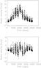 |
Fig. 10 Upper panel: RVtot versus time for Set 1, best sampling. The solid line is the sinusoidal fit derived as described in Sect. 4.1. Lower panel: RV after correction using the sinusoidal fit method, assuming no Ca noise. |
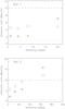 |
Fig. 11 Upper panel: detection limits versus the sampling for the sinusoidal fit procedure, Set 1, and no noise on reconstructed Ca. Detection limits are computed using the correlation-based method (stars, orange), and the LPA method (squares, blue). Lower panel: same for Set 2. |
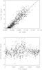 |
Fig. 12 Upper panel: total RV signal versus the measured Ca index (978 data points). The rms RV is 2.50 m/s. The linear fit is represented as a solid line. Lower panel: corrected RV signal using the linear fit. The rms RV is 1.05 m/s. |
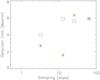 |
Fig. 13 Detection limits versus sampling for the corrected signal using measured Ca (Set 2) for the correlation-based method (stars, orange), and the LPA method (squares, blue). |
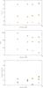 |
Fig. 14 Upper panel: rms versus sampling for the corrected RV using measured Ca (Set 2) for four RV noise levels (orange), for the original spots+plages RV signal (green, +, our objective after correction) and the total RV signal (red, x, values before correction). Middle panel: same for the power. Lower panel: same for the correlation with the spots+plages RV signal on the same sampling. |
4.2. Correction using Ca-RV correlation
4.2.1. The method
The method is as follows. We fit the RVtot versus Ca (either observed or reconstructed, for the sampling we are interested in) curve by a linear function, as shown in Fig. 12. We obtain for example, RVfit = −47.4 + 546.8Ca for the observed Ca (Set 2), which is substracted from the original RVtot to provide a corrected RV (hereafter RVcorr). This is done for various samplings as in the previous section. The law relating Ca and RV is computed for each sampling, i.e. on the available data points. The resulting RVcorr is then analysed as previously: the detection limits and the three criteria (rms, power, and correlation) defined in Sect. 2.1.4 are computed.
4.2.2. Results with observed Ca
We compute the detection limits using this method for the observed Ca time series and Set 2. The detection limits after correction are shown in Fig. 13. They are compared with those shown in the sixth panel (before correction) and second panel (our objective) in Fig. 4. The detection limits are significantly improved after correction, as they are now well below 10 MEarth instead of being in the 10−20 MEarth regime. With the best sampling and most optimistic method, we find detection limits around 2−3 MEarth, i.e. above 1 MEarth. They are between 4 and 7 MEarth for the LPA method. However, these values are all larger than the detection limit for RVsppl, Set 2. With the worst sampling, the detection limits are in the range 5−10 MEarth, i.e. in the Super-Earth regime or above.
The parameters defined in Sect. 2.1.4 are shown in Fig. 14. The rms RV and power after correction are significantly improved (in the range 1−1.2 m/s), but remain far from the RVsppl values. The correlation of the corrected RV with RVsppl is not improved at all.
The comparison with the sinusoidal fit approach (Sect. 4.1) shows that the detection limits are very similar for the correlation method and slightly improved for the LPA method. The rms RV after correction is indeed slightly better (for the best sampling of Set 2, we obtain 1.07 m/s instead of 1.30 m/s), and the periodogram in the period range we are interested in presents less power. However, the improvement is marginal and does not allow us to reach the 1 MEarth regime. The two methods applied to this signal therefore perform similarly.
4.2.3. Results with reconstructed Ca
The analysis above was based on Set 2 and thus with a smaller set of data points than Set 1. The aim of this section is to estimate the results on longer time series and different Ca noise levels. To do so, it is necessary to use the reconstructed Ca series defined in Sect. 3.2 and then test the quality of the correction for various noise levels in Ca. The impact of various effects will be studied in the following section. We also compare the results obtained with Set 2 with the previous ones (including with the sinusoidal fit method). Using these reconstructed Ca time series, we can apply the correction technique described in Sect. 4.2.1 on any samplings and RV noise levels, either on the full cycle Set 1, the restricted sample of points Set 2 (to compare with the previous results) or shorter durations (Set 3 and Set 4).
The detection limits are shown in Fig. 15 and are summarised for the best sampling of Set 1 and Set 2 in Table 2. The errorbar-like symbols on the figure represent the maximum range covered by the detection limits over ten realisations and not the uncertainty on the average detection limit (which would be smaller). This range is slightly underestimated, given the number of realisations.
When we assume no noise on the Ca index, we find that the correction allows us to reach detection limits around 1 MEarth for sampling up to one point every eight days: these detection limits are slightly above those obtained for RVsppl (see Fig. 4) but are very similar, which is expected since we build the RV and Ca from the same ff, which are supposed to be perfectly known. However, the sinusoidal fit method could not recover that performance, even with no Ca noise.
With a very good S/N on Ca (σhigh, second row in Fig. 15), a 1 MEarth planet could be detected in certain cases (i.e. some realisations, but not all of the Ca noise): the range covered by the detection limits usually covers a 1 MEarth planet. However, for a given data set and sampling, a large fraction of the noise realisations leads to detection limits that are above 1 MEarth, usually in the domain of a few MEarth.
For a median S/N on Ca (50), the detection limits are almost all above 1 MEarth, from a few MEarth planets to 10 MEarth for the best samplings and Set 1 or Set 2. For more degraded temporal samplings, it is possible to obtain detection limits as large as 10 MEarth or larger for some realisations of the Ca noise, and they can reach 20 MEarth in the worst cases. For low S/N on Ca, the detection limits are even larger and are usually in the 10−20 MEarth range.
The corresponding criteria (rms RV, correlation with RVsppl and power, described in Sect. 2.1.4) are shown in Fig. 16. Assuming no noise, the rms RV after correction is very close to the RVsppl rms, as is the power, and the correlation with RVsppl is good (around 0.7), although not perfect. When adding noise to the Ca index, the parameters are further from the RVsppl levels as the S/N noise on Ca decreases. For a medium S/N, for example, the power is still more than one order of magnitude larger than for RVsppl and has almost not decreased at all for the worst S/N. Finally, we note that when assuming no Ca noise, the correlation between the corrected RV and the RVsppl time series is significantly improved, but it is only marginally improved even with the σhigh noise level. This shows that even where the correction is good enough to suppress most of the convective component to improve the detection limits to a very good level, the resulting RV still contains some contaminations in addition to the theoretical RVsppl: it will make the extraction of the spots and plages components difficult.
4.2.4. Notes on the Ca noise
As for the sinusoidal method, we observe a large dispersion in detection limits (see Table 2) depending on the Ca noise realisation. The results are therefore sensitive to the realisation of the Ca noise. This will be studied in more detail in Sect. 5.1.
 |
Fig. 15 Detection limits versus sampling for the corrected signal using reconstructed Ca for the correlation-based method (stars, orange), and the LPA method (squares, blue). Each row corresponds to a different Ca noise level (from top to bottom: no noise, σhigh, σmed, σlow). Each column corresponds to a data set (from left to right: from Set 1 to Set 4). The errorbar symbols indicate the minimum value and maximum values for each detection limit, computed for ten realisations of the Ca noise. |
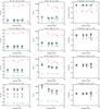 |
Fig. 16 Left panels: rms versus sampling for the corrected RV using the measured Ca for four data sets (blue, the errorbar symbols indicating the minimum and maximum values), the original spots+plages RV signal (green, +, our objective after correction) and the total RV signal (red, x, values before correction). The two latter rms are shown for Set 1 and Set 2. Each row corresponds to a different Ca noise level (from top to bottom: no noise, σhigh, σmed, σlow). Middle panels: same for the power. Right panels: same for the correlation with the spots+plages RV signal on the same sampling. |
The residuals after a linear fit of the observed Ca index versus RV are slightly larger than what would be expected from the noise level of 0.6% (see Sect. 3.1) and correspond to a S/N of about 50. There are several possible origins for this, in addition to the measurement errors:
-
Although both RV and Ca are verywell correlated with the filling factor of plages and network, theattenuation of the convective blueshift ΔV and theCa emission vary from one plage to another, andfrom one location inside a plage to another. The measuredCa includes that effect but not the reconstructedRV (and therefore RVtot), for which a constant ΔV (i.e.independent of the local magnetic field or plage size) was chosento be representative of the average structures and applied. Theimpact of this effect is studied in Sect. 5.
-
Although we expect the largest plages to exhibit the largest ΔV and be the brightest, there is probably a dispersion in this relationship.
-
The observations (reconstructed RV and Ca) were taken on the same day but not exactly at the same time. As a result, the Sun rotated by a few degrees between the time at which the Ca index was measured and the time at which the structures used to build the reconstructed RV times series were identified from MDI/SOHO data. We estimate that a typical difference of 12 hours between both measurements would introduce a noise of about 0.7%. This represents an upper limit.
We note that the detection limits for the observed Ca are within the range obtained for the medium S/N of 50. Although the S/N on observed Ca is about 166, i.e. closer to the high S/N considered in this section, the actual S/N to consider is closer to 50 due to the effects mentionned above. There is therefore a good agreement between the observed Ca and reconstructed Ca detection limits.
4.3. Conclusion
When compared with the sinusoidal fit approach in the same conditions (reconstructed Ca with no noise) the Ca-RV correlation method provides much better detection limits and allows levels below 1 MEarth with no noise or very good Ca S/N to be reached. This test is, however, very optimistic as we are dealing with ideal conditions, with detection limits below 1 1 MEarth for the best sampling and no Ca noise, and above 1 MEarth in the presence of noise (except for a few realisations of the high S/N case), up to almost 7 MEarth for a low Ca S/N and good sampling. Realistic detection limits should lie between those obtained with realistic Ca noise and the results for observed Ca. We could interpret these results as follows: on observed Ca (i.e. noisy data), both correction methods provide similar (but poor) detection limits because the residual rms RV is dominated by the large dispersion in Ca. In an ideal case, the sinusoidal fit approach is not adapted because of the variation of activity level at various time scales (whose residuals dominate the signal), while the Ca-RV correlation approach takes these into account and is therefore more adapted.
5. Robustness of the Ca-RV correction
In this section, we study in more detail some possible limitations of the Ca-RV method that seems the most promising.
5.1. Impact of the Ca noise and sampling realisation
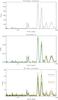 |
Fig. 17 Upper panel: periodogram of the RV before correction for Set 1, best sampling. Middle panel: periodogram of the 10 Ca time series for that sampling and a medium Ca S/N. Lower panel: periodogram of the 10 RV series after correction. The horizontal lines on the right indicate the maximum power in the periodograms. |
As noted in Sect. 4.1, there is a strong impact of the Ca noise realisation on the resulting detection limits (Fig. 15). Figure 17 illustrates why we have such a dispersion. The upper panel shows the periodogram of the RV signal before correction for Set 1 (best sampling). The middle panel shows the periodograms for the 10 Ca time series for a medium Ca S/N. We observe a variation of the maximum amplitude of power of the order of ±10%. The lower panel shows the ten periodograms of the RV after correction. The power is significantly reduced compared to the upper panel, by a factor of at least 15. However, the maximum power varies by a factor 2 (as the detection limit for this configuration shown in Table 2) over these ten realisations. This level is directly correlated with the LPA detection limits (correlation larger than 0.99), while the maximum Ca power (middle panels) is strongly anti-correlated with this level (correlation of −0.98). The variations of amplitude from one Ca realisation to another is relatively small, but it is amplified on the corrected RV due to its small level. The detection limits drastically depend on the actual Ca noise realisation (in addition to the Ca S/N). Hence, for a given target, it is not possible to give precise detection limits because the Ca noise realisation may change. A reference is the highest value obtained for different Ca noise realisations.
The temporal sampling also has a strong impact (Fig. 15). It regards the choice of the selected days of the original sampling (when choosing one point every four days, for example), but also the choice of the four-month gap. As an illustration, we computed the detection limits for the observed Ca and Set 1 with the gap located at a different period during the year and obtained a significantly different detection limit: for the best sampling (one point every day), differences are of the order of 0.2 MEarth but can reach several MEarth for one point for every 20 day-sampling. It is beyond the scope of this paper to perform a systematic study of the detection limits for a large number of gap positions. However, we point out that this impact can be quantified in advance and various samplings tested, while the Ca noise realisation is not controlled.
5.2. Impact of the varying Ca intensity and convective blueshift attenuation
Both RV and Ca are very well correlated with ff of plages and network. However, there is an effect that is present in the measured Ca (Sect. 3.1) but not in the RV simulations: different plages have different properties. The previous section, being ideal, may therefore be too optimistic. The reconstructed RVs are indeed computed assuming that the convective blueshift attenuation (Paper II) is constant (i.e. the same for all structures): a constant ΔV was applied to all structures, representative of all structures on average. Furthermore, the Ca emission also varies from one structure to another, which is not taken into account either in the above Ca reconstruction, while it is present in the measured Ca. In this section, we quantify the impact of this effect. If the difference between the results obtained when using observed Ca index and when using reconstructed Ca index is due to this effect, we expect the impact to be of the order of 1.5 MEarth for the correlation method (2.9 MEarth for LPA) for a good temporal sampling as derived from the difference between Fig. 13 and Fig. 15 (considering Set 2 and high Ca S/N).
We first compute a modified RV , which takes into account a variable ΔV: we use the law ΔV = 55.log A + 0.21, with A the size of the structure in part-per-million (ppm) of the solar disk derived from the Fig. 7 of Meunier et al. (2010b).
As for the Ca variations, although it is well known that larger structures exhibit larger emission levels, we are not aware of a precise law relating the two. We consider here two methods:
-
Method 1: Worden et al. (1998)derived Ca intensities for several categories ofplage and network structures. We used their values for twoextreme categories (each covering a large range of sizes) and weconsidered a linear relation between the size and Ca: aCa contrast of 0.33 for 95 ppm structures and acontrast of 0.95 for the largest ones (about 4000 ppm). This leadsto an index Ca1.
-
Method 2: Meunier (2003) derived the magnetic flux Φ as a function of the size A from the network to plage sizes. We used that relation log Φ = 1.175log A + 18.7 to derive the magnetic flux. We then found the average magnetic field B in each structure from A and Φ. Finally, we used the relation between the magnetic field B and the Ca emission derived by Ortiz & Rast (2005) Ca = 0.016 B0.66. This leads to an index Ca2.
Ca1 and Ca2 are used to produce new ff times series, which are then used as the original one in the procedure to build reconstructed Ca (see Sect. 3.2). The resulting reconstructed Ca are close to the original one. With the first approach, the correlation between the two is 0.97, with an rms on the difference of about 1%; with the second approach, the correlation between the two is 0.99, with an rms on the difference of 0.4%.
We first compute detection limits after correction for Set 1 and no noise to study the impact of these effects and compare them with Fig. 15 (upper left-hand panel). With the LPA method, if we replace RVtot by RV, the detection limits are slightly increased by ~0.2−0.9 MEarth. If we replace the reconstructed Ca by Ca1, the same detection limits are increased by ~1−1.9 MEarth (0.2−0.7 MEarth for Ca2). However, if we replace both RVtot by RV and Ca by Ca1, the results are very similar to those presented in Sect. 4.2, and the variation is between −0.1 and 0.3 MEarth (same variation for Ca2). The results are qualitatively similar for the correlation-based method. This shows that taking into account one of the effects (either variable ΔV or variable Ca intensity) modifies the detection limits and increases them, but taking into account none or both (i.e. considering consistent dependences) provides similar results. This shows that we can be confident of the performances of the Ca-RV method in excellent noise and sampling conditions (i.e. allowing a 1 MEarth detection limit to be reached) since on real data the RV and Ca series will be consistent.
Finally, we make the same computation considering high S/N Ca noise and no noise, and compare the results with variable Ca intensity with the results of Sect. 4.2 obtained for Set 2. The detection limit for Ca with no noise is 0.5 MEarth for both methods, while it is 2.7 and 4.0 MEarth, respectively for the correlation and the LPA methods. When taking into account a varying Ca intensity in the reconstructed Ca, the detection limits are increased to 2.6 and 3.5 MEarth, respectively for the correlation and the LPA methods for the first method (Ca1). The agreement with the observed Ca detection limit is therefore quite good. The improvement is not as good for the second method (Ca2), as the detection limits are only increased to 1.6 and 2.3 MEarth. However, there is an uncertainty associated to the Ca noise realisation (in that case for the observed Ca).The same computation with a high S/N Ca noise shows that the upper limit (over ten realisations) of the detection limits are larger when taking into account a varying Ca variation, so that there is a better agreement with the observed Ca detection limits. However, except for the first method (Ca1) and LPA, they remain below the observed Ca detection limits, showing that this effect may not explain everything.
We conclude that this effect has therefore a small impact on the detection limits computed with the reconstructed RV and that the use of consistent convective blueshift attenuation and Ca emission gives similar results (i.e. either both variable RV and Ca or both constant RV and Ca).
5.3. Impact of an error on the Ca-RV laws
In this section and the next one, we study the impact of possible errors in the estimation of the Ca-RV law as deduced from measured Ca index. We consider the uncertainties on the linear fit of RV versus Ca. The important parameter is the slope. We compute the detection limits for the “no Ca noise” case, but use the slope plus or minus the 1-σ uncertainty on the slope. The detection limits are not significantly different from the computation made in Sect. 3.2.1, showing that the uncertainty of the law estimation does not significantly impact the result, including when the sampling is bad. We therefore conclude that the use of a slope varying within the errorbars does not significantly impact the results.
5.4. Impact of the presence of a planet on the correction
We study the impact of the presence of a planet at the period we are interested in or at other periods on the RV-Ca law, i.e. on the correction. We first consider a planet with a period of 200, 480, and 600 day, with no Ca noise, Set 1, and masses between 1 and 10 MEarth. The RV-Ca laws derived from the simulation are slightly different from the no planet case, but the slopes are compatible with the no planet case at the 1-σ level in almost all cases. This should not significantly impact the detection limits. For a high S/N Ca noise level, the slope of the RV-Ca law tends to be smaller than in the no planet case. For degraded sampling the uncertainties increase and therefore the slopes become compatible in most cases, the difference being mostly significant for the one-day sampling: part of the difference in detection limits may be due to an error in the law estimation and therefore in the correction process. Overall, the impact of the presence of a planet on the correction itself is small.
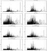 |
Fig. 18 First row: periodogram of the total RV signal added to the RV signal due to a 1 MEarth at 1.2 AU after correction (method described in Sect. 4.2), with the Set 1 sampling (all days) and no Ca noise. The vertical dotted line indicates the position of the planet peak. The left panel shows the best detection case out of 7 planet phases, while the right panel shows the worse case. Second row: same for Set 2 and no Ca noise. Third row: same for Set 1, high Ca S/N, and a Ca realisation leading to a detection limit below 1 MEarth. Fourth row:same for Set 1, high Ca S/N, and a Ca realisation leading to a detection limit above 1 MEarth for the correlation method (1.6 MEarth). Power is in arbitrary unit but on the same scale on all plots. |
6. Periodograms after correction
In this section, we give a few examples of periodograms after correction in the presence of a 1 MEarth at 1.2 AU. In the case of excellent sampling and Ca S/N conditions, the detection limits are below 1 MEarth when no planet is present in the RV signal. The upper panels of Fig. 18 show the RV after the correction described in Sect. 4.2 for a 1 MEarth at 1.2 AU for the Set 1 sampling (all days) and no Ca noise. In this computation the planet is present before the correction. The detection limits are 0.7 MEarth for the correlation method and 0.3 MEarth for the LPA method. This plot should be compared to those shown in Fig. 6, especially the middle panel (for RVsppl, i.e. what we should obtain if the correction was perfect). We note that the amplitude of the planet peak is sensitive to the phase and therefore show two extreme cases (out of seven configurations). In both cases, there is a clear peak due to the planet, which would not have been visible without the correction.
The second rows show the same plots for Set 2 (all days, no noise), for which the detection limits were 0.5 MEarth for both methods. Here again we see the planet peak, although in the worst phase configuration the planet peak is hardly above the adjacent peaks. This shows that, for some phases, the detection of a 1 MEarth would probably be difficult to make, but it should be possible in some cases.
The two last rows show the same plots again, but for Set 1 and two realisations of the Ca noise, for the high Ca S/N considered in Sect. 3 (about 130). We discussed previously the high sensitivity to the Ca noise realisation, with the detection limit below or above 1 MEarth depending on the realisation (Table 2). The first of these two rows corresponds to a case for which we find a detection limit below 1 MEarth: in the two extreme cases for the phase configurations, the planet peak is clearly above the nearby peaks. The last row corresponds to a realisation for which the detection limit is above 1 MEarth. For the worst phase configuration the planet peak cannot be identified (justifying the detection limit above 1 MEarth). However, for certain phase configurations, it is still possible to make a detection.
We estimated that to get a significant fraction of detection of a 1 MEarth at 1.2 AU (above 50% of all phases and Ca realisations), it is necessary to have at least 1000 observations and a Ca S/N above 130. With a S/N around 100, this proportion falls to 30−40%, and for a smaller number of points, the fraction is also typically well below 10%, even with a very good Ca S/N level.
7. Discussion and conclusion
We have first compared detection limits by quantifying the impact of the presence of solar-type activity on the detectability of Earth-mass exoplanets as simulated in Paper II. We confirm that for a very good sampling and without convection it is possible to reach detection limits below 1 MEarth. However, the presence of convection dominates the signal leading to detection limits above 6 MEarth at best, and usually well above 10 MEarth. The amplitude of the convection component would have to be reduced by a factor of at least 10 to allow the 1 MEarth regime to be reached. We also confirm that in the domain 0−10 cm/s the RV noise has a small impact on the result.
We tested two methods using Ca emission index to correct the RV signal from the convection contribution. The first one is based on a sinusoidal fit of the temporal variations of Ca, the second on the direct relationship between Ca index and the RV signal. We obtained the following results:
-
The two methods perform similarly but poorly when theCa noise is high. They both lead to an improvementof the detection limits (down to 2.5 MEarth in the bestcases, but above 10 MEarth for very low S/N), but do notallow 1 MEarth to be reached.
-
For very low Ca noise, the second method performs better, as the first remains dominated by the residuals due to the fact that the solar activity can not be modelised by a sinusoidal function. However, an excellent Ca noise level is required to reach the 1 MEarth regime (S/N significantly larger than 100).
-
The detection limits are very sensitive to the exact realisation of the temporal sampling (which can be tested in advance for actual stellar observations) and to the actual Ca noise realisation. It is therefore not possible to precisely predict detection limits after correction.
-
The use of reconstructed Ca to test methods is possible, although one has to keep in mind its limitations and, in particular, the dependence of RV and Ca on magnetic fields.
-
The presence of a planet in the signal impacts the detection limits, mostly because of the additional power at certains periods, especially for excellent Ca S/N5. The impact is not directly related to the quality of the correction.
We also find that the original level of the convection contribution must be small in order to achieve an excellent performance of the correction, especially if the Ca measurements are noisy. For a small convection amplitude, the determination of the RV-Ca law is probably less precise than for a high level of convection, as there is a smaller amplitude of variation of RV (which is then less dominated by the convection component, because the spot and plage components have an average of zero). The correction to be made, however, is also smaller. We conclude that the smaller the convection level, the easier the correction.
For Sun-like conditions, i.e. similar activity, convection level, and orientation, the use of the Ca-RV relationship to evaluate the correction of the convective contribution is more effective than the use of a sinusoidal fit on the Ca variations. A planet 1 MEarth or below could be detected after performing a correction of the RV times series if both the temporal sampling and the noise on the Ca index are excellent. We estimate that a probability larger than 50% to detect a 1 MEarth at 1.2 AU is obtained with more than 1000 observations and a Ca S/N larger than 130. We emphasise that this study is limited to the solar case, assuming an edge-on star. Further studies will consider other types of
stars, seen under different configurations. This study is based on several simplifying assumptions, which may overestimate the capability to correct for the activity signal, for example, constant spot and plage temperatures and constant convection inhibition in active regions for all features, as well as the Zeeman effect (Reiners et al. 2013).
Ca emission index, corresponding to the integration of the flux over 1 Å and centred on the Ca II K line, measured at the Sacramento Peak Solar Observatory.
The total RV variations also include the contributions from spots and plages, which are not proportional to the surface covered by plages: because these RV components change sign at the central meridian (where the surface and convective component are maximal), these spot and plage contributions add some dispersion to the relationship between total RV and surface. This contribution is small when the convection dominates the RV signal.
S. Keil, priv. comm.
For small data sets the temporal sampling is also slightly different due to the addition of a small random shift (see Sect. 2.1.1).
The detection limit computations assume that there is no planet in the observed signal. If a planet is present and increases the power in the periodogram at a given period, the detection limit is increased accordingly at this period (because the planet peak is interpreted as due to another source, either noise or stellar), independently of the correction.
Acknowledgments
We acknowledge the Sacramento Peak Observatory of the U.S. Air Force Philips Laboratory and S. Keil for providing the Ca index and informations on these data. We acknowledge financial support from the French Programme National de Planétologie (PNP, INSU). We also acknowledge support from the French National Research Agency (ANR) through project grant NT05-4_44463.
References
- Aigrain, S., Pont, F., & Zucker, S. 2012, MNRAS, 419, 3147 [NASA ADS] [CrossRef] [Google Scholar]
- Boisse, I., Bouchy, F., Hébrard, G., et al. 2011, A&A, 528, A4 [NASA ADS] [CrossRef] [EDP Sciences] [Google Scholar]
- Desort, M., Lagrange, A.-M., Galland, F., Udry, S., & Mayor, M. 2007, A&A, 473, 983 [NASA ADS] [CrossRef] [EDP Sciences] [Google Scholar]
- Dumusque, X., Lovis, C., Ségransan, D., et al. 2011, A&A, 535, A55 [NASA ADS] [CrossRef] [EDP Sciences] [Google Scholar]
- Hatzes, A. P. 2002, Astron. Nachr., 323, 392 [NASA ADS] [CrossRef] [Google Scholar]
- Isaacson, H., & Fischer, D. 2010, ApJ, 725, 875 [NASA ADS] [CrossRef] [Google Scholar]
- Lagrange, A.-M., Desort, M., & Meunier, N. 2010, A&A, 512, A38 [NASA ADS] [CrossRef] [EDP Sciences] [Google Scholar]
- Lanza, A. F., Bonomo, A. S., & Rodonò, M. 2007, A&A, 464, 741 [NASA ADS] [CrossRef] [EDP Sciences] [Google Scholar]
- Lovis, C., Dumusque, X., Santos, N. C., et al. 2011, A&A, submitted [arXiv:1107.5325] [Google Scholar]
- Meunier, N. 2003, A&A, 405, 1107 [NASA ADS] [CrossRef] [EDP Sciences] [Google Scholar]
- Meunier, N., Desort, M., & Lagrange, A.-M. 2010a, A&A, 512, A39 [NASA ADS] [CrossRef] [EDP Sciences] [Google Scholar]
- Meunier, N., Lagrange, A.-M., & Desort, M. 2010b, A&A, 519, A66 [NASA ADS] [CrossRef] [EDP Sciences] [Google Scholar]
- Meunier, N., Lagrange, A.-M., & De Bondt, K. 2012, A&A, 545, A87 [NASA ADS] [CrossRef] [EDP Sciences] [Google Scholar]
- Ortiz, A., & Rast, M. 2005, Mem. Soc. Astron. It., 76, 1018 [Google Scholar]
- Reiners, A., Shulyak, D., Anglada-Escude, G., et al. 2013, A&A, accepted [arXiv:1301.2951] [Google Scholar]
- Saar, S. H., & Donahue, R. A. 1997, ApJ, 485, 319 [NASA ADS] [CrossRef] [Google Scholar]
- Worden, J. R., White, O. R., & Woods, T. N. 1998, ApJ, 496, 998 [Google Scholar]
All Tables
Detection limits for the best sampling of Set 1 and Set 2 for selected conditions and a planet at 1.2 AU.
All Figures
|
Fig. 1 Upper panels: reconstructed series for spots+plages RVsppl (left) and all components including convection RVtot (right). Set 3 and Set 4 are indicated by horizontal arrows. Set 1 and Set 2 cover the whole range. Lower panels: corresponding periodograms. The periodograms are in the same arbitrary units. |
| In the text | |
|
Fig. 2 Periodograms (zoom on the wide peaks) of the RV variations produced by a 100 (respectively 75, 50, 25, 5 from top to bottom) MEarth planet at a phase of zero and period of 480.1 days, for Set 3, solid line (respectively dashed, dotted, dot-dashed, dot-dot-dot-dashed). The vertical line indicates the theoretical position of the peak. The arrows indicate the position of the planet peak for each planet mass. |
| In the text | |
|
Fig. 3 Detection limits versus sampling for RVsppl (i.e. no convection), Set 1, and a planet at 1.2 AU. Different RV noise levels are considered: no noise (stars), 1 cm/s (diamonds), 5 cm/s (triangle), and 10 cm/s (square). Each panel corresponds to a detection limit method. |
| In the text | |
|
Fig. 4 Two first rows: detection limits versus sampling for the spots+plages RV signal for Sets 1 to 4, no RV noise, for the correlation-based method (stars, orange), and the LPA method (squares, blue). Two last rows: same for the total RV signal. |
| In the text | |
|
Fig. 5 Upper panel: rms of the RV signal versus the sampling for zero RV noise, for the spots+plages RV signal (green), and for the total RV signal (red) for Set 1 (stars), Set 2 (diamonds), Set 3 (triangle), and Set 4 (squares). Middle panel: same for the total power computed from the periodogram. Lower panel: same for the correlation with the spots+plages RV signal corresponding to the same sampling. |
| In the text | |
|
Fig. 6 Upper panel: periodogram of a 1 MEarth at 1.2 AU with the Set 1 sampling (all days). The vertical dotted line indicates the position of the planet peak. Middle panel: same for the RVsppl added to the signal of this planet. Lower panel: same for the RVtot added to the signal of this planet. Power is in arbitrary unit but on the same scale on all plots. |
| In the text | |
|
Fig. 7 Upper left panel: detection limits versus sampling for a modified RVtot corresponding to a convection contribution ten times smaller than the solar one for Set 1. Detection limits are computed using the correlation-based method (stars, orange), and the LPA method (squares, blue). There is no noise level on the RV signal. Upper right panel: same for Set 3. Lower panels: same for a convection contribution five times smaller than the solar one. |
| In the text | |
|
Fig. 8 Upper panel: detection limits versus planet period for RVsppl (Set 1, no RV noise, daily sampling). Detection limits are computed using the correlation-based method (stars, orange), and the LPA method (squares, blue). Middle panel: same for RVtot. Lower threshold: correlation threshold for RVsppl (stars) and RVtot (diamonds). The vertical dashed lines indicate the one-year period position. |
| In the text | |
|
Fig. 9 From top to bottom: observed Ca emission index (Sacramento peak, upper panel) and reconstructed Ca index with various noise levels (see Sect. 3.2), for all available data points. |
| In the text | |
|
Fig. 10 Upper panel: RVtot versus time for Set 1, best sampling. The solid line is the sinusoidal fit derived as described in Sect. 4.1. Lower panel: RV after correction using the sinusoidal fit method, assuming no Ca noise. |
| In the text | |
|
Fig. 11 Upper panel: detection limits versus the sampling for the sinusoidal fit procedure, Set 1, and no noise on reconstructed Ca. Detection limits are computed using the correlation-based method (stars, orange), and the LPA method (squares, blue). Lower panel: same for Set 2. |
| In the text | |
|
Fig. 12 Upper panel: total RV signal versus the measured Ca index (978 data points). The rms RV is 2.50 m/s. The linear fit is represented as a solid line. Lower panel: corrected RV signal using the linear fit. The rms RV is 1.05 m/s. |
| In the text | |
|
Fig. 13 Detection limits versus sampling for the corrected signal using measured Ca (Set 2) for the correlation-based method (stars, orange), and the LPA method (squares, blue). |
| In the text | |
|
Fig. 14 Upper panel: rms versus sampling for the corrected RV using measured Ca (Set 2) for four RV noise levels (orange), for the original spots+plages RV signal (green, +, our objective after correction) and the total RV signal (red, x, values before correction). Middle panel: same for the power. Lower panel: same for the correlation with the spots+plages RV signal on the same sampling. |
| In the text | |
|
Fig. 15 Detection limits versus sampling for the corrected signal using reconstructed Ca for the correlation-based method (stars, orange), and the LPA method (squares, blue). Each row corresponds to a different Ca noise level (from top to bottom: no noise, σhigh, σmed, σlow). Each column corresponds to a data set (from left to right: from Set 1 to Set 4). The errorbar symbols indicate the minimum value and maximum values for each detection limit, computed for ten realisations of the Ca noise. |
| In the text | |
|
Fig. 16 Left panels: rms versus sampling for the corrected RV using the measured Ca for four data sets (blue, the errorbar symbols indicating the minimum and maximum values), the original spots+plages RV signal (green, +, our objective after correction) and the total RV signal (red, x, values before correction). The two latter rms are shown for Set 1 and Set 2. Each row corresponds to a different Ca noise level (from top to bottom: no noise, σhigh, σmed, σlow). Middle panels: same for the power. Right panels: same for the correlation with the spots+plages RV signal on the same sampling. |
| In the text | |
|
Fig. 17 Upper panel: periodogram of the RV before correction for Set 1, best sampling. Middle panel: periodogram of the 10 Ca time series for that sampling and a medium Ca S/N. Lower panel: periodogram of the 10 RV series after correction. The horizontal lines on the right indicate the maximum power in the periodograms. |
| In the text | |
|
Fig. 18 First row: periodogram of the total RV signal added to the RV signal due to a 1 MEarth at 1.2 AU after correction (method described in Sect. 4.2), with the Set 1 sampling (all days) and no Ca noise. The vertical dotted line indicates the position of the planet peak. The left panel shows the best detection case out of 7 planet phases, while the right panel shows the worse case. Second row: same for Set 2 and no Ca noise. Third row: same for Set 1, high Ca S/N, and a Ca realisation leading to a detection limit below 1 MEarth. Fourth row:same for Set 1, high Ca S/N, and a Ca realisation leading to a detection limit above 1 MEarth for the correlation method (1.6 MEarth). Power is in arbitrary unit but on the same scale on all plots. |
| In the text | |
Current usage metrics show cumulative count of Article Views (full-text article views including HTML views, PDF and ePub downloads, according to the available data) and Abstracts Views on Vision4Press platform.
Data correspond to usage on the plateform after 2015. The current usage metrics is available 48-96 hours after online publication and is updated daily on week days.
Initial download of the metrics may take a while.