| Issue |
A&A
Volume 550, February 2013
|
|
|---|---|---|
| Article Number | A58 | |
| Number of page(s) | 18 | |
| Section | Cosmology (including clusters of galaxies) | |
| DOI | https://doi.org/10.1051/0004-6361/201118388 | |
| Published online | 28 January 2013 | |
The galaxy stellar mass function and its evolution with time show no dependence on global environment⋆
1 Astronomical Department, Padova University, 35122 Padova, Italy
e-mail: This email address is being protected from spambots. You need JavaScript enabled to view it.
2 INAF – Astronomical Observatory of Padova, 35122 Padova, Italy
3 Observatories of the Carnegie Institution of Science, Pasadena, CA, USA
4 School of Physics and Astronomy, University of Nottingham, Nottingham NG7 2RD, UK
5 INAF – Astronomical Observatory of Trieste, 34143 Trieste, Italy
6 Department of Astronomy & Astrophysics, University of Chicago, Chicago, IL, USA
7 INAF – Astronomical Observatory of Arcetri, 50125 Firenze, Italy
Received: 3 November 2011
Accepted: 31 October 2012
Abstract
We present an analysis of the galaxy stellar mass function in different environments at intermediate redshift (0.3 ≤ z ≤ 0.8) for two mass-limited galaxy samples. We use the IMACS Cluster Building Survey (ICBS; M∗ ≥ 1010.5 M⊙) to study cluster, group and field galaxies at z = 0.3–0.45, and the ESO Distant Cluster Survey (EDisCS; M∗ ≥ 1010.2 M⊙) to investigate cluster and group galaxies at z = 0.4–0.8. Our analysis thus includes galaxies with masses reaching just below that of the Milky Way. Excluding the brightest cluster galaxies, we show that the shape of the mass distribution does not seem to depend on global environment, Our two main results are: (1) Galaxies in the virialised regions of clusters, in groups, and in the field follow similar mass distributions. (2) Comparing the ICBS and EDisCS mass functions to mass functions in the local universe, we detect evolution from z ~ 0.4–0.6 to z ~ 0.07 in the sense that the population of low-mass galaxies has grown with time with respect to the population of massive galaxies. This evolution is independent of environment, i.e., the same for clusters and the field. Furthermore, considering only cluster galaxies, we find that no differences can be detected in their mass functions either within the virialised regions, or when we compare galaxies inside and outside the virial radius. Finally, we find that red and blue galaxies have different mass functions. However, the shapes of the mass functions of blue and red galaxies do not seem to depend on their environment (clusters groups and the field).
Key words: galaxies: evolution / galaxies: formation / galaxies: clusters: general / galaxies: luminosity function, mass function
This paper includes data gathered with the 6.5 m Magellan Telescopes located at Las Campanas Observatory, Chile.
© ESO, 2013
1. Introduction
In standard Λ cold dark matter (ΛCDM) cosmological models, cold dark matter haloes form from the gravitational collapse of dark matter around peaks in the initial density field. Haloes assemble hierarchically in such a way that smaller haloes merge to form larger and more massive ones in dense environments (Mo & White 1996; Sheth & Tormen 2002). According to the current paradigm of galaxy formation, galaxies form within these haloes due to the cooling of hot gas. Haloes and galaxies evolve simultaneously and the evolution of a galaxy is driven by the evolution of its host halo. If the halo is accreted by a larger halo, the galaxy will also be affected and, in some cases, the galaxy’s diffuse hot gas reservoir may be stripped, thus removing its fuel for future star formation (e.g. Larson et al. 1980; Balogh et al. 2000; Weinmann et al. 2006; van den Bosch et al. 2008). The evolution can also be governed by the interplay between smooth and clumpy cold streams, disk instability, and bulge formation. Intense and relatively smooth streams can maintain an unstable dense gas-rich disk. Instability with high turbulence and giant clumps is self-regulated by gravitational interactions within the disk (see, e.g., Dekel et al. 2009, and references therein). Galaxies may also experience major mergers, which transform late-type galaxies into early-type ones with a central bulge component (e.g. Driver et al. 2006; Drory & Fisher 2007). Mergers drive gas towards the centres of galaxies, where it can trigger a burst of star formation and fuel the central black hole, the feedback from which can heat the remaining gas and eventually quench star formation (e.g. Mihos & Hernquist 1996; Wild et al. 2007; Pasquali et al. 2008; Schawinski et al. 2009).
Several studies have shown that there are additional external disturbances acting mainly on galaxies in dense environments, and generally preventing the survival of spiral structure. For example, ram pressure (Gunn & Gott 1972; Bekki 2009) is a gas-driven drag force capable of stripping a galaxy of much of its interstellar gas, hence preventing the formation of new stars. Galaxy harassment (Moore et al. 1996; Boselli & Gavazzi 2006) is a mechanism that strips a galaxy of part of its mass and may change its morphology as a consequence of frequent high speed encounters. Harassment has the potential of changing any internal property of a galaxy within a cluster, including its gas distribution and content, the orbital distribution of its stars, and its overall shape. Finally, cluster tidal forces (Byrd & Valtonen 1990) can act with different efficiency depending on the environment in such a way that gas-rich field galaxies infalling into larger structures may be transformed into gas-poor lenticular galaxies.
For all these reasons, galaxies are expected to be strongly influenced by the environment in which they reside during their evolution. It is also broadly accepted that the evolution of a galaxy depends very strongly on its stellar mass. Kauffmann et al. (2003) found that colour, specific star formation rate, and internal structure are strongly correlated with galaxy stellar mass. Pasquali et al. (2009) demonstrated that the star formation and AGN activity of galaxies have a much stronger dependence on stellar mass than on halo mass. Thomas et al. (2010) argued that the formation of early-type galaxies is environment-independent and driven only by self-regulation processes and intrinsic galaxy properties such as mass.
Distinguishing the separate contribution of environmental processes and processes driven by intrinsic galaxy properties is clearly critical to understanding galaxy evolution. In the “nature versus nurture” debate, mass represents the primary “intrinsic property” expected to be closely related to the initial conditions. The “environment”, on the other hand, represents all the possible external processes that can influence galaxies in their evolution.
There are many papers in the literature where the effect on galaxies of the global environment and mass are analysed separately (see e.g. Guo et al. 2009; Iovino et al. 2010; Mercurio et al. 2010; Peng et al. 2010). The basic idea is to study variations in galaxy properties as a function of mass fixing the environment, or as a function of the environment fixing the galaxy mass. However, studies of galaxy properties as a function of mass often ignore the possibility that the galaxy mass distribution itself may vary with environment.
In this paper we investigate whether (and how) the effects of mass and environment are related and whether the environment can influence the galaxy masses themselves. In particular, we will consider the galaxy stellar mass distribution in different environments. Galaxy stellar masses can be estimated reasonably easily, even though the uncertainties are still relatively large, but there is not a unique way to describe the environment.
Different methods of estimating stellar masses agree reasonably well within the errors. Examples include Bell & de Jong (2001), who use a relation between the stellar mass-to-light ratio and the galaxy colour, and Bolzonella et al. (2010), who use a SED fitting technique based on the code Hyperzmass, a modified version of the photometric redshift code Hyperz (Bolzonella et al. 2000). Note, however, that different choices of the IMF, stellar population synthesis model, SFR history, metallicity and extinction law can systematically affect the stellar mass estimates (see, e.g., Marchesini et al. 2009; Muzzin et al. 2009; Conroy et al. 2010).
When describing or quantifying the environment, it is possible to refer to either global or local environments. As discussed in detail in Muldrew et al. (2012), there is no universal environmental measure and the most suitable method generally depends on the spatial scale(s) being probed. Concerning the global environment, galaxies are commonly subdivided into, for instance, superclusters, clusters, groups, the field and voids, which can be expected to roughly correspond to the galaxies’ host halo mass. The local environment is generally described using estimates of the local density, which can be calculated following several definitions and methods.
Several works have focused on the galaxy mass distribution and its evolution in the field, but very little is known about the galaxy stellar mass function in clusters. Studies focused on field galaxies (Drory et al. 2005; Gwyn & Hartwick 2005; Fontana et al. 2006; Bundy et al. 2006; Pozzetti et al. 2007; Drory et al. 2009; Baldry et al. 2012), present the mass function for the global field galaxy population at different redshifts and obtain consistent results. Fontana et al. (2004, 2006); Bundy et al. (2006); Borch et al. (2006); and Pozzetti et al. (2010) demonstrated that galaxies with M∗ ≥ 1011 M⊙ exhibit relatively modest evolution in their total mass function from z = 1 to z = 0. This implies that the evolution of relatively-massive objects (with masses close to the local characteristic mass) is essentially complete by z ~ 1. On the other hand, the mass functions of less massive galaxies were found to evolve more strongly than those of massive ones, displaying a rapid rise since z ~ 1. Readers interested in the evolution of the mass function at z > 1 should see Elsner et al. (2008); Kajisawa et al. (2009); Marchesini et al. (2009); Caputi et al. (2011); González et al. (2011) and Mortlock et al. (2011).
There have been a number of mass function studies separating galaxies by morphology. Galaxies with different morphologies and star formation histories can contribute in different ways to the mass function. Broadly speaking, galaxies can be separated into different populations such as early and late types according to their star formation histories (using rest-frame colours, SEDs or spectra) or their structure (using quantitative structural parameters or visual morphologies). Balogh et al. (2001) analysed the environmental dependence of the luminosity function and the associated stellar mass function of passive and star forming galaxies in the Two Micron All Sky Survey. They found that the mass function of field star-forming galaxies has a much steeper high mass end than that of field passive galaxies. In clusters, however, both star-forming and passive galaxies have a steep high mass end.
Subdividing field galaxies according to their colour in the local universe (Baldry et al. 2004, 2006, 2008) and at intermediate redshifts (Borch et al. 2006; Bolzonella et al. 2010) it has been found that the mass function is bimodal, with early-type galaxies dominating at high masses and late-types mostly contributing at intermediate and low masses. Moreover, these authors also find that the mass functions of early- and late-type galaxies evolve differently with redshift.
Vulcani et al. (2011) studied for the first time the mass function of cluster galaxies, finding quite a strong evolution with redshift. Clusters in the local universe are proportionally more populated by low mass galaxies than clusters at high z. This study concluded, first, that the mass growth caused by star formation plays a crucial role in driving the observed evolution; second, that this star-formation-driven mass growth must be accompanied by infall of galaxies onto clusters; and third, that the mass distribution of the infalling galaxies may be different from that of cluster galaxies. To test this last result, a comparison was made between the mass function of cluster galaxies and that of field galaxies found in the literature. Preliminary analysis suggests that at high masses (log M∗/M⊙ ≥ 11), the mass functions of field and cluster galaxies at high-z seem to have rather similar shapes. However, the situation at intermediate/low masses is not clear since different field studies give quite different results in this mass range. Using the field mass function of Ilbert et al. (2010), it seems as if field galaxies have a steeper mass function than cluster galaxies at intermediate/low masses, thus suggesting significant environmental mass segregation. In contrast, the results of Bundy (2005)1 suggest that there are no large differences between the mass distributions of galaxies in different environments at high z. Based on these results, it remains unfortunately unclear whether field and cluster galaxies have similar or different mass distributions. It is also important to note that the preliminary results presented in Vulcani et al. (2011) were obtained using inhomogeneous data and slightly different redshift ranges, so definite conclusions cannot be drawn.
On the theoretical side, Moster et al. (2010) found a correlation between the stellar mass of the central galaxy and the mass of the dark matter halo. Using N-body simulations, they found that the clustering properties of galaxies are predominantly driven by the clustering of the halos and subhaloes in which they reside, and provided a model to predict clustering as a function of stellar mass at any redshift. This result could also suggest that the total (central + satellites) mass function may depend on environment. However, the correlation between the total galaxy stellar mass function and the mass of the parent halo has not yet been studied. It would be very interesting to understand whether simulations predict a mass segregation with environment, considering the initial and evolved halo mass and how they predict the evolution with redshift in different environments. This would allow us to understand the role of the halo mass in influencing the evolution of galaxy masses. This analysis is deferred to a forthcoming paper (Vulcani et al., in prep.).
2. Aims of this work
So far, observational studies have shown that in different environments early- and late-type galaxies are present in different proportions and follow different mass distributions. As mentioned above, the theoretical expectation is that the stellar mass of central galaxies depends on the environment. This may also raise the expectation that the total mass function could be different in different environments. The main goal of our work is to test this possibility by studying the stellar mass distribution as a function of the halo mass. Note that to compare mass functions of galaxies in clusters, groups and the field means also to compare mass functions of galaxies hosted in haloes with different masses.
We want to investigate whether the mass function is “universal” and, if this is the case, how this came about. The main questions of this paper are: (i) do observations suggest that the mass function at intermediate redshifts is driven by the halo mass? (ii) does the mass function of red and blue galaxies separately depend on halo mass? (iii) does the evolution of the mass functions depend on global environment (a proxy for halo mass)? Alternatively, we wish to know whether it is possible for the galaxy mass distribution to be unaffected by where the galaxies form and which halo they grow in. If that is the case, we will need to ask whether there is some mechanism imprinting the same stellar mass distribution on all galaxies, regardless where they are.
The analysis presented in this work is complementary to that presented in Vulcani et al. (2012). There we analysed the role of the local density in shaping the mass function, using a nearest-neighbour-based density measure largely independent of dark matter halo mass (Muldrew et al. 2012). In that paper, we addressed the following questions: does the mass function depend on local density at low- and intermediate-z, both in clusters and in the field? How does the mass function change with local density? These two papers therefore address different points. The two ways to define the “environment” are not equivalent and provide different information (the effect of halo masses versus local phenomena). Sometimes the differences between local and global environment are subtle and confusing, and it is therefore possible that part of the results presented in this paper will surprise the reader. They are not in line with what it is generally expected. We will show here that, even if the mass function does depend on local density (as we show in Vulcani et al. 2012), the differences in local density distributions in clusters compared to the field are insufficient to induce a difference in the mass functions in these global environments. Thus, the investigation of the dependence of the mass functions on global environment that we carry out in this paper is an independent test of whether the global environment alone is able to produce a difference in the galaxy mass function. Note that Vulcani et al. (2012) brings together the results of both studies, contrasting the role of global and local environments in shaping the mass function.
List of ICBS clusters analysed in this paper.
The study of the mass functions of galaxies has only been developed in the last years, while much more effort has been devoted to characterising luminosity functions. The literature contains a variety of papers that carefully analyse luminosity functions, their evolution with redshift and their dependence on environment. At first sight, it seems reasonable to expect that the stellar mass function will simply mirror the luminosity function behaviour, given that stellar masses are derived from luminosities. For this reason it is commonly thought that results derived from the luminosity function would also apply to the mass function. However, this is not necessarily the case. A simple linear correlation between mass and luminosity does not exist: not all galaxies have the same mass-to-light ratio. In cases such as passively-evolving old galaxies the mass-to-light ratios are fairly constant, but galaxies with different star formation histories can have significantly different mass-to-light ratios. As a consequence, the luminosity function does not provide, in general, direct information on the mass function (see Appendix A). It is therefore not unreasonable to expect that the environmental effects on the luminosity and mass functions may not be the same.
Furthermore, it is important to note that the samples used when analysing luminosity and mass functions should be assembled following different criteria. Traditionally, luminosity functions are studied in magnitude-limited samples, where a cut in luminosity is performed. In contrast, mass function studies require, ideally, mass-limited samples, including all galaxies more massive than a given limit regardless of their colour or morphological type. As discuss in Appendix B of Vulcani et al. (2011), the choice of a magnitude limit implies a natural mass limit below which the sample is incomplete. Hence the mass distribution derived from a magnitude-limited sample is meaningless because it is affected by incompleteness: galaxies will be missing at masses below the limit corresponding to the mass of a galaxy with the reddest colour and the faintest magnitudes in the sample. It is therefore clear that mass-limited samples are needed in environmental and evolutionary studies of the mass function,
The goal of this paper is thus to compare the galaxy stellar mass distribution in cluster regions, cluster infalling regions, groups, and the field using homogeneous data. This will allow us to establish whether and by how much the total galaxy stellar mass function depends on global environment at a fixed redshift. Note that it is interesting to consider the mass function not only in clusters but also in their outskirts, where galaxies will have time to become part of the clusters themselves by z = 0. We will also divide galaxies by colour, separating the mass functions of star-forming and passive galaxies in all environments.
The paper is organized as follows. In Sect. 3 we present the two surveys we use in our analysis, the IMACS Cluster Building Survey (ICBS) and the ESO Distant Cluster Survey (EDisCS). In Sect. 4 we define the different environments. Section 5 shows the results, with Sect. 5.1 presenting the galaxy stellar mass function as a function of the global environment, Sect. 5.2 compares our findings with some results from the literature, quantifying the evolution of the mass function in different environments We then analyse the galaxy stellar mass function in clusters (Sect. 5.3), dividing it by colour (Sect. 5.4). In Sect. 6 we discuss our results, explaining their implications for the evolution of mass functions (Sect. 6.1), and the dependence of the mass distribution on galaxy properties (Sect. 6.2). We then contrast the different roles played by the global and local environments in shaping the mass function (Sect. 6.3). Finally, in Sect. 7 we summarise our results.
Throughout this paper, we assume H0 = 70 km s-1 Mpc-1, Ωm = 0.30, and ΩΛ = 0.70. The adopted initial mass function (IMF) is that of Kroupa (2001) in the mass range 0.1–100 M⊙. All magnitudes used in this paper are Vega magnitudes.
3. Data set
In this paper, we take advantage of two different surveys to carry out an analysis of the mass function. We use ICBS data to characterise galaxies at intermediate redshifts (0.3 ≤ z ≤ 0.45) and EDisCS data to study a large sample of galaxies at 0.4 ≤ z ≤ 0.8.
The ICBS provides homogeneous spectroscopic data of galaxies in several environments. Spectroscopy yields accurate redshifts, and therefore the membership to the different environments is well established.
EDisCS contains a much larger sample of cluster and group galaxies, although spectroscopic redshifts are available for only a subset of them. Photometric redshifts are therefore used, even though they are less reliable. In Appendix A of Vulcani et al. (2011), we showed that the galaxy mass function determined using photo-z’s and photo-z membership agrees with the mass function determined using only spectroscopic members and spectroscopic completeness weights in the mass range across which they overlap.
3.1. ICBS
The ICBS (Oemler et al. 2012a) is focused on the study of galaxy evolution and infall onto clusters from a clustercentric radius R ~ 5 Mpc to the cluster inner cores. Data have been acquired using the wide field of the Inamori-Magellan Areal Camera and Spectrograph (IMACS) on the Magellan-Baade telescope for four fields containing clusters at intermediate redshift.
The ICBS aims at defining a homogeneous sample of clusters by selecting the most massive cluster per comoving volume at any redshift. Clusters were selected using the Red-Sequence Cluster Survey method Gladders & Yee (2000), either from the RCS itself, or from the Sloan Digital Sky Survey in regions of the sky not covered by the RCS. As described in Oemler et al. (2012a), direct imaging in the griz bands was obtained for two of the fields with the f/2 camera of IMACS. Imaging in the BVRI bands was obtained for the other two fields using the Wide Field CCD camera on the du Pont Telescope. In addition, very deep r-band photometry, complete to r = 25.0, was obtained for all fields with IMACS. Spectroscopic targets were selected from r-band photometry down to a limiting magnitude r = 22.5 for all fields.
The IMACS f/2 spectra have an observed-frame resolution of 10 Å full width at half-maximum with a typical S/N ~ 20−30 per resolution element in the continuum. In each 28′ diameter IMACS field, spectra for 65% of the galaxies brighter than r ~ 22.5 were taken on the 6.5 m Baade Telescope at Las Campanas. Of those observed, only about 20% failed to yield redshifts, or turned out to be stars. Details of the data and its analysis are presented in Oemler et al. (2012a) and Oemler et al. (2012b).
The data discussed in this paper come from four fields containing rich galaxy clusters at z = 0.33, 0.38, 0.42 and 0.43, as well as other structures at different redshifts. In this paper, we restrict our analysis to ICBS galaxies in the redshift range 0.3 < z < 0.45 in all environments. This was done in order to focus on a limited redshift range so that a common magnitude and mass limit could be set up to z = 0.45. Consequently, we have analysed data for galaxies in these four rich clusters together with field and group galaxies within the chosen redshift range in all four fields. In Table 1 we provide information for the four target clusters. Velocity dispersions (σ) were calculated using ROSTAT (Beers et al. 1990). Galaxies were accepted as cluster members if their redshifts placed them within ± 3σ from the cluster redshift.
Since the projected density of cluster/supercluster members is low at the large clustercentric distances probed by the ICBS, our sample necessarily includes ~ 1000 “field” galaxies at redshifts 0.2 < z < 0.8 in each survey field. This gives us the opportunity to compare the evolution of cluster and field galaxies over this redshift range. Figure 1 shows the redshift distribution for the four fields RCS 1102, RCS 0221, SDSS 1500, and SDSS 0845 in the redshift range considered. The cluster regions (±3σ from the cluster redshift) are also indicated.
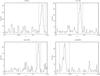 |
Fig. 1 ICBS: redshift distribution in the four fields observed by the survey: RCS0221, RCS1102, SDSS0845, and SDSS1500. The cluster regions ( ± 3σ from cluster redshift) are also indicated (vertical dotted lines). |
Absolute magnitudes were determined using INTERREST (Taylor et al. 2009) from the observed photometry. The tool interpolates the rest-frame magnitudes from the observed photometry in bracketing bands (see Rudnick et al. 2003). The code uses a number of template spectra to carry out this interpolation. Rest-frame colours are derived from the interpolated rest-frame apparent magnitudes.
Galaxy stellar masses are derived using the relation between M/LB and rest-frame (B − V) colour given in Bell & de Jong (2001) (1)For a Bruzual & Charlot model with solar metallicity and a Salpeter (1955) IMF (0.1–125 M⊙), aB = −0.51 and bB = 1.45. Since our broadband photometry does not cover the entire field of the redshift survey, galaxies without the required photometry had synthetic colours calculated from the flux-calibrated IMACS spectra. The error in the measured masses is ~0.3 dex. All our masses are scaled to a Kroupa (2001) IMF, by adding –0.19 dex to the logarithmic value of the Salpeter masses.
The magnitude completeness limit of the ICBS spectroscopy is r ~ 22.5. At the redshift limit of the ICBS sample, z ~ 0.45, we determine the value of the mass of a galaxy with an absolute B magnitude corresponding to r = 22.5, and a rest-frame colour (B − V) ~ 1, the reddest colour of galaxies in ICBS clusters. From this we determine that the ICBS mass completeness limit at the redshifts of interest is M∗ = 1010.5 M⊙. The colour distributions of both the ICBS and EDisCS samples (see Figs. 6 and 7) confirm that they are complete and unbiased down to our mass limit.
In this paper, galaxies are given weights proportional to the inverse of the spectroscopic incompleteness. Since the main galaxy property that we wish to analyse is galaxy stellar mass, we compute the incompleteness correction taking into account the number of galaxies for which an estimate of the mass is available. Above our mass limit, 91% of all galaxies brighter than r = 22.5 with available spectroscopy have mass estimates2.
The incompleteness correction depends on both the apparent magnitude and the position in the field. We subdivided each field into three different regions according to their distance from the centre of the main cluster (R/R200 ≤ 1;1 < R/R200 ≤ 2; and R/R200 > 2)3 and we then determined the completeness weights in 0.4 r magnitude bins around each galaxy as the ratio of the number of galaxies with a spectroscopic redshift and a given mass to the number of galaxies in the original photometric catalog.
For all clusters we excluded the Brightest Cluster Galaxy (BCG), identified as the most luminous cluster member, because its characteristics could alter the general conclusions. The final mass-limited ICBS sample consists of 596 galaxies with M∗ ≥ 1010.5 M⊙ in all environments. After correcting for incompleteness, this number becomes 1295.
3.2. EDisCS
The EDisCS multiwavelength photometric and spectroscopic survey of galaxies (White et al. 2005) was developed to characterise both the clusters themselves and the galaxies within them. It observed 20 fields containing galaxy clusters at 0.4 < z < 1. These clusters were selected from the Las Campanas Distant Cluster Survey (LCDCS) catalog (Gonzalez et al. 2001).
For all 20 fields deep optical multiband photometry obtained with FORS2/VLT (White et al. 2005) and near-IR photometry obtained with SOFI/NTT is available. ACS/HST mosaic F814W imaging was also acquired for 10 of the highest redshift clusters (Desai et al. 2007). FORS2/VLT was additionally used to obtain spectroscopy for 18 of the fields (Halliday et al. 2004; Milvang-Jensen et al. 2008).
The FORS2 field covers R200 for all clusters with the exception of cl 1232.5–1250, for which the field only covers 0.5R200 (Poggianti et al. 2006). The R200 values were computed from the velocity dispersions by Poggianti et al. (2008).
Photometric redshifts were computed for each object from both optical and infrared data using two independent codes, a modified version of the publicly-available Hyperz (Bolzonella et al. 2000) and the code of Rudnick et al. (2001), as modified in Rudnick et al. (2003) and Rudnick et al. (2009). The accuracy of both methods is σ(δz) ~ 0.05–0.06, where  Photo-z membership (see also De Lucia et al. 2004; and De Lucia et al. 2007, for details) was determined using a modified version of the technique first developed in Brunner & Lubin (2000). The probability P(z) for a galaxy to be at redshift z is integrated in a slice Δz = ± 0.1 around the cluster redshift to give Pclust for the two codes. A galaxy was rejected as a member if Pclust is smaller than a certain probability Pthresh for either code. For each cluster Pthresh was calibrated using the spectroscopic redshifts to maximise the efficiency of spectroscopic non-member rejection while retaining at least ~ 90% of the confirmed cluster members independently of rest-frame (B − V) or observed (V − I).
For EDisCS galaxies, stellar masses were estimated following Bell & de Jong (2001) and then scaled to a Kroupa (2001) IMF. Total absolute magnitudes were derived from the photo-z fits (Pelló et al. 2009) and rest-frame luminosities calculated using the methods of Rudnick et al. (2003) and Rudnick et al. (2006), as presented in Rudnick et al. (2009). As a check, stellar masses for spectroscopic members were also estimated using the kcorrect tool (Blanton & Roweis 2007)4. These masses agree with the photo-z based ones within the errors. A detailed discussion on stellar mass estimates and the consistency between different methods can be found in Vulcani et al. (2011).
List of EDisCS clusters and groups analysed in this paper.
To build the EDisCS mass-limited sample, we used all photo-z members of all clusters and groups. Using the photo-z membership selection instead of the spectroscopic one we maximise sample size while still retaining adequate quality. Furthermore, the spectroscopic magnitude limit (I = 22 or I = 23, depending on redshift) would correspond a stellar mass limit M∗ = 1010.6 M⊙ (Vulcani et al. 2010). Using photo-z’s allows us to push the mass limit to significantly lower values. Our adopted conservative magnitude completeness limit for the EDisCS photometry is I ~ 24 (the sample remains close to 90% complete at I ~ 25, White et al. 2005). For the most distant cluster in our sample (cl 1216.8–1201 at z ~ 0.8) the stellar mass of a galaxy with an absolute B magnitude corresponding to I = 24 and (B − V) ~ 0.9, the reddest colour, is M∗ = 1010.2 M⊙. We take this value as the EDisCS stellar mass completeness limit for the photo-z sample. As before, BCGs were excluded. Table 2 presents the list of clusters used and some basic properties.
Definitions adopted to characterise the different environments for ICBS (upper panel) and EDisCS (bottom panel).
Number of galaxies in each environment above the stellar mass completeness limits.
The final mass-limited EDisCS sample of galaxies with M∗ ≥ 1010.2 M⊙ consists of 2962 objects.
4. Definition of the different environments
The mass-limited galaxy samples defined above were divided into different environments. For the ICBS survey, the cluster galaxy sample includes all the cluster members, i.e., galaxies lying within 3σ of the cluster redshift. These are then subdivided according to their clustercentric distance. Galaxies in the “cluster virialised regions” are defined as those with R/R200 ≤ 1, and those with R/R200 > 1 are said to live in the “cluster outskirts”. Moreover, we further subdivide the cluster core (virialised region) into three zones: inner parts (R/R200 ≤ 0.2), intermediate parts (0.2 < R/R200 ≤ 0.6), and outer parts (0.6 < R/R200 ≤ 1).
The group galaxy sample was defined from a group catalog constructed using the standard method of Huchra & Geller (1982). We identify groups by a friends-of-friends technique where the linking velocity distance used to connect friends is 350 km s-1 and the projected linking length DL scales with the incompleteness of the data as
![Mathematical equation: $$ D_{\rm L} = D_0 \left[ I(r,\alpha,\delta) \frac{\int_{-\infty}^{M_{\rm pair}} \Phi(M) {\rm d}M}{\int_{-\infty}^{M_{\rm lim}} \Phi(M) {\rm d}M} \right]^{-1/2}\cdot\vspace*{-2mm} $$](/articles/aa/full_html/2013/02/aa18388-11/aa18388-11-eq133.png) In this formula, D0 = 0.40 Mpc is the linking length at a fiducial redshift zfid = 0.30. I(r,α,δ) is the incompleteness of the data at a given r magnitude and position in the field, as described in Oemler et al. (2012a). The numerator is the integral of the galaxy luminosity function to the limiting absolute magnitude at the distance of the galaxy pair, corrected for galaxy evolution as described in Oemler et al. (2012b) and the denominator is the integral of the galaxy luminosity function to the absolute magnitude limit at the fiducial redshift.
In this formula, D0 = 0.40 Mpc is the linking length at a fiducial redshift zfid = 0.30. I(r,α,δ) is the incompleteness of the data at a given r magnitude and position in the field, as described in Oemler et al. (2012a). The numerator is the integral of the galaxy luminosity function to the limiting absolute magnitude at the distance of the galaxy pair, corrected for galaxy evolution as described in Oemler et al. (2012b) and the denominator is the integral of the galaxy luminosity function to the absolute magnitude limit at the fiducial redshift.
Although this method makes efficient use of all the data, it produces groups whose properties vary systematically with redshift because of the definition of DL. However, since we only consider a fairly narrow redshift range, this drawback does not affect our analysis.
Finally, we call “field galaxies” all those galaxies that are not cluster members.
Within the EDisCS sample we are able to reliably identify only two main environments: (1) clusters, with their virialised regions, outskirts, and the inner, intermediate and outer regions defined as before, and (2) groups. EDisCS clusters are defined as systems with velocity dispersion σ > 400 km s-1. Cluster members are selected using the photo-z technique described above. Groups are defined as systems with at least eight spectroscopic members and velocity dispersions in the range 150 km s-1 ≤ σ ≤ 400 km s-1. Group members are also selected using the photo-z method. Table 3 summarises the definitions adopted to characterise the different environments, separately for ICBS (upper panel) and EDisCS (bottom panel).
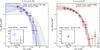 |
Fig. 2 Observed mass functions and Schechter (1976) function fits for galaxies in the different environments. Left panel: ICBS cluster regions (black crosses and solid line) and field (blue empty stars and dotted line). Right panel: EDisCS clusters (black crosses and solid line) and groups (red filled hexagons and dotted line). Mass functions are normalised using the total integrated stellar mass above the mass completeness limits. Errorbars on the x-axis represent the width of the bin. Errorbars on the y-axis are computed combining the Poissonian errors (Gehrels 1986) and the uncertainties due to cosmic variance and cluster-to-cluster variations. Shaded area represent 1σ errors on the Schechter fits. The labels at the top show both the observed and completeness-weighted galaxy numbers for ICBS, while for EDisCS only observed numbers are given. The K–S probabilities are also shown as percentages. The bottom left in-sets in each panel show the M∗ and α Schechter fit parameters with 1σ errors. No significant differences are evident between the galaxy stellar mass distributions in different environments. For ICBS, similar results are also obtained comparing the cluster regions and the non-cluster regions (plot not shown). |
Note that the definitions of groups are not the same in both samples. However, this does not affect our findings since we never compare them directly.
As mentioned above, we exclude the BCGs from both samples when we consider the cluster regions because they could alter the general trends. The properties of BCGs are in many aspects very different from those of other galaxies, and they the subject of many specific studies (e.g., Aragón-Salamanca et al. 1998; Whiley et al. 2008; Fasano et al. 2010).
Above the mass limit of M∗ ≥ 1010.5 the ICBS sample contains 178 cluster galaxies in the virialised regions, 177 in the cluster outskirts, and 241 field galaxies, 90 of which belong to groups (see Table 4 for completeness-corrected numbers). The EDisCS sample has 268 galaxies in the cluster virialised regions, 749 in the outskirts, and 620 group galaxies above a mass limit of M∗ ≥ 1010.2 (see Table 4).
5. Results
Using the mass-selected samples defined above we have built histograms characterising the mass distribution of galaxies located in different environments The width of each mass bin is 0.2 dex. For the ICBS sample each galaxy is weighted by its spectroscopic incompleteness correction. Note that we do not need to apply this correction for EDisCS galaxies since we are using photo-z defined samples. The errorbars on the x-axis represent the width of the bins. The errorbars on the y-axis are computed combining the uncertainties derived from Poisson errors (Gehrels 1986) and those resulting from cosmic variance5. Throughout this paper all mass functions are normalised using the total integrated stellar mass above the mass completeness limit (Rudnick et al. 2009). so that the total galaxy stellar mass in each histogram is equal to 1. Such a normalisation allows us to focus our analysis on the shape of the mass functions and not on the number density, which is obviously very different across the different environments.
To quantify the differences between different mass functions, we perform Kolmogorov-Smirnov (K–S) tests which tell us whether we can disprove the null hypothesis that two data sets are drawn from the same parent distribution. Since the standard K–S test does not consider (in)completeness when compiling the cumulative distributions (i.e., it assigns weight 1 to each object), we modified it in such a way that the relative importance of each galaxy in the cumulative distribution depends on its weight. Obviously, in the case of photo-z samples (EDsiCS) all galaxies have weight = 1 so using the modified test is equivalent to using the standard one. For ICBS data we use the modified K–S test to take into account the spectroscopic incompleteness.
We recall that a “positive” (statistically significant) K–S result provides robust proof that the two distributions are different, but a negative K–S result does not mean that the distributions are identical. Therefore, visual inspections of the mass distributions, in particular at their high-mass ends, could be useful.
In the analysis that follows we always use the mass limit of M∗ ≥ 1010.5 M⊙ for the ICBS survey, while for EDisCS we use its own mass limit (M∗ ≥ 1010.2 M⊙) for internal comparisons but the ICBS mass cut when comparing both surveys.
5.1. The mass function in different environments is very similar
First of all, we wish to characterise the galaxy stellar mass distribution of galaxies located in different global environments, to see whether it depends on the region in which galaxies reside.
To begin, we compare galaxies in the cluster virialised regions (R/R200 ≤ 1) with field and group galaxies. Using ICBS data only we can compare the most widely different environments, the cluster virialised regions and the field. The left panel of Fig. 2 shows no significant differences between the shapes of the galaxy stellar mass distributions for these two environments. The K–S test is unable to reject the null hypothesis that the two distributions are drawn from the same sample (PK − S ~ 46%). A visual inspection of the mass functions provides confirmation of the K–S result: their shapes are similar, within the errors, in both environments. To increase the quality of the data statistics, we also compare the galaxies in the cluster virialised regions with those in the field+cluster outskirts. Again, we do not find detectable differences (PK − S ~ 40%; plot not shown).
In the right panel of Fig. 2 we compare EDisCS cluster and group galaxies reaching lower masses than before (M∗ ~ 1010.2 M⊙). Yet again, there is no clear evidence of a dependence of the shape of the mass function on the environment. The K–S test is still inconclusive (PK − S ~ 21%) even with the better statistics provided by the larger samples. A visual inspection clearly reveals that the shapes of the mass functions are very similar.
Photometric redshifts can be uncertain, especially for blue galaxies (see Rudnick et al. 2009). In principle, photo-z errors could bias the stellar mass functions derived for EDisCS galaxies. However, we checked, first, that the magnitudes at which Rudnick et al. (2009) found discrepancies in the galaxy luminosity functions correspond to lower stellar masses than those considered here (our Mg is always brighter than − 20.2). In addition, the photo-z counts are fully consistent with the statistically background-subtracted counts for both red and blue galaxies. Furthermore, for the mass range in common, the mass function determined from photo-z’s is in agreement (within the errors) with the mass function determined using only spectroscopic members after taking into account spectroscopic completeness (Vulcani et al. 2011). These tests provide reasonable confidence in the results obtained using photo-z techniques.
For both ICBS and EDisCS, the results concerning the low mass end of the mass functions are statistically robust. At the high mass end, however, the size of the uncertainties do not allow a reliable characterisation of the mass functions and their putative differences. It is therefore not possible to conclude whether the apparent similarities are real or simply due to the size of the errors.
The strength of our results can be double checked by considering analytical fits to the mass functions using a least-square-fitting method. Assuming that the number density Φ(M) of galaxies with stellar mass M∗ can be described by a Schechter (1976) function, the galaxy stellar mass function can be written as  (2)where M = log (M∗/M⊙), α is the low-mass-end slope, Φ∗ the normalisation and
 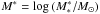 corresponds to the characteristic stellar mass
  at which the mass function exhibits a rapid change in slope. Schechter function fits consider only galaxies above our conservative mass completeness limits. Table 5 gives the best-fit Schechter function parameters for the mass functions of galaxies in different environments (see also Sects. 5.2 and 5.3).
Note that because the mass functions have been normalised, the values of Φ∗ do not provide meaningful information on the true galaxy density. Since we are only concerned about comparing the shapes of the mass functions, in what follows we only carry out comparisons involving M∗ and α.
Allowing all the parameters to be fitted freely, we find that the mass functions in different environments show comparable α and M∗. Explicitly, given that the errors in these two parameters are correlated, we explored a grid of α and M∗ and calculated the corresponding χ2 values and from these the likelihood of two mass functions having the same pair of parameters. We found that that the fitted mass functions agree within 1σ. This exercise gives additional support to our finding that the shapes of the mass functions do not seem to depend on the global environment. This result is particularly robust for EDisCS since the better statistics allow for good constraints on the Schechter function parameters6.
It is important to point out that, in agreement with previous studies (e.g., Bell et al. 2003; Baldry et al. 2008), we find that a Schechter function is not able to adequately describe the highest mass end of the cluster and group mass functions. A sort of “bump” or excess is seen at M∗ ~ 1012.3 M⊙ in both clusters and groups. However, a Schechter function fits well the distributions for masses below M∗ ~ 1012 M⊙. It could be argued that for EDisCS this bump may be caused by contamination by interlopers since we use photo-z’s to determine membership. However, most of the high-mass photo-z members are also spectroscopic members, and galaxies in the bump do not show larger photo-z errors than lower mass galaxies. We note that a similar bump has also been detected in the mass function of the low-z spectroscopic cluster galaxy sample in the WINGS survey (WIde-field Nearby Galaxy-cluster Survey, Fasano et al. 2006. See Sect. 5.2).
In the ICBS survey we have also considered more narrowly-defined environments separately. When comparing the mass functions of galaxies in clusters, groups and the field outside groups we fail to detect any obvious differences in their shapes. Even though the statistical uncertainty is larger and the mass functions are thus noisier, the PK − S is always inconclusive.
Confidence in the robustness of our results is reinforced by the fact that the mass functions derived from EDisCS and ICBS independently show a similar lack of environmental dependence. These two surveys have different strengths. ICBS provides spectroscopically-defined relatively small samples with very reliable separation into the different environments. On the other hand, EDisCS provides a larger galaxy sample extending to lower masses, albeit affected by the intrinsic photo-z uncertainties.
These results seem be at odds with the findings of Kovač et al. (2010). They studied ~ 8500 galaxies from the zCOSMOS-bright redshift survey in the COSMOS field. They found that the shape of the stellar mass function is different for group, field and isolated galaxies up to z ~ 0.7 at least. Their stellar mass function shows an upturn at low masses in the group environment. They also found that more massive galaxies preferentially reside in groups. However, their samples reach much lower masses than ours (down to M ⋆ ~ 109.5 M⊙) and, more importantly, their selection of group and field galaxies are very different from the one adopted here. Therefore, a direct comparison of the results cannot be made at this point.
We finish this section by noticing that, even though the mass functions appear to have similar shapes in all the environments studied here, there is a hint that a small difference may be present. The mass functions seem to extend to different maximum masses, the so-called mass function cut-off. In the ICBS survey the most massive galaxies in clusters have M∗ ~ 1011.9 M⊙, while in the field they have M∗ ~ 1011.7 M⊙, and in groups M∗ ~ 1011.6 M⊙. In EDisCS, the virialised regions of clusters seem to contain galaxies as massive as M∗ ~ 1012.5 M⊙, while cluster outskirts only reach M∗ ~ 1012.1 M⊙ and groups M∗ ~ 1012.3 M⊙.
5.2. The evolution of the mass functions is very similar in different environments
We have shown in this paper that for masses M∗ ≥ 1010.2 − 10-10.5 M⊙ the shape of the galaxy stellar mass function at intermediate redshifts does not seem to depend on the global environment in which galaxies reside. We have carried out a complementary study in the local universe (Calvi et al., in prep.) using a mass-limited sample (M∗ ≥ 1010.25 M⊙) of galaxies from the Padova Millennium Galaxy and Group Catalog (PM2GC) (Calvi et al. 2011) and the WINGS survey. This work also shows that cluster, group and field galaxies at low-z have comparable mass functions7. As the next natural step, we investigate now whether the evolution of the galaxy stellar mass function changes with environment.
In Vulcani et al. (2011), we compared cluster galaxy stellar mass functions at low and high-z using WINGS and EDisCS data and found a strong evolution from z ~ 0.8 to z ~ 0, which we attributed primarily to mass growth due to star formation in late-type cluster galaxies and infalling galaxies. We found that the shape at M∗ > 1011 M⊙ does not evolve but the mass function at high redshift is flat below M∗ ~ 1010.8 M⊙, while in the Local universe it flattens out at significantly lower masses. The population of M∗ = 1010.2 − 1010.8 M⊙ galaxies must have grown significantly between z = 0.8 and z = 0.
Pozzetti et al. (2010), using data from the zCOSMOS-bright 10k spectroscopic sample, quantified the evolution of the mass function in the field since z ~ 1. They used data from Baldry et al. (2008), who selected galaxies from the NewYork University Value-Added Galaxy Catalog sample as reference at z = 0. They found a continuous increase with time in the mass function for log M/M∗ < 11 and a much slower increase at higher masses.
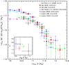 |
Fig. 3 Comparison between the mass function in clusters and in the field at different redshifts. At low-z, red filled squares: PM2GC (general field); cyan empty squares: Baldry et al. (2008) (general field); blue empty triangles: WINGS (clusters). At intermediate-z, black crosses: ICBS (field); black skeleton triangles: ICBS (clusters). At higher-z: magenta skeleton stars: Pozzetti et al. (2010) (field); green filled triangles EDisCS (clusters). Mass functions are normalised using the total integrated stellar mass in the range 11.2 < log M∗/M⊙ < 11.7 (the last bin in the ICBS). Errorbars and in-set as in Fig. 2. The evolution of the shape of the mass function seems not to depend on environment, being similar in clusters and in the field. However, in all cases the amount of growth as a function of cosmic time is different at the low- and high-mass ends. |
We are now in the position to compare the evolution of the mass function in clusters with that in the field. In Fig. 3, we examine the evolution from z ~ 0.4−0.8 to z ~ 0. At z ~ 0.07 we show the mass functions for WINGS clusters and Baldry et al. (2008) and PM2GC for the general field. At z ~ 0.4, those of clusters and field from ICBS. At z ~ 0.6, the mass functions shown are those of EDisCS clusters and Pozzetti et al. (2010) field (priv. comm.).
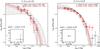 |
Fig. 4 Observed mass functions and corresponding Schechter function fits for galaxies at different clustercentric distances (R/R200 ≤ 1 and R/R200 > 1) for the ICBS survey (left panel) and EDisCS (right panel). Black crosses and solid lines represent cluster regions, and red empty stars and dotted lines the cluster outskirts. Mass function normalisations, errorbars, labels and in-sets are as in Fig. 2. In both panels, no statistical differences are detected between the mass functions of galaxies located at different clustercentric distances. |
Perhaps unexpectedly, the evolution does not depend on global environment: it seems similar in clusters and the field. At similar redshifts, the shape of the mass functions of field and cluster galaxies overlap quite significantly, within the errors. As cosmic time increases, the number of galaxies at low and intermediate masses grows with respect to the number of massive galaxies. This growth is similar in clusters and in the field.
However, it is hard to quantify accurately the evolution from z ~ 0.4 and z ~ 0.6 to z = 0, due to the uncertainties. In Table 5, best-fit Schechter function parameters are given for the WINGS, PM2GC, ICBS and EDisCS samples. For these, stellar mass estimates and mass functions are derived in the same way and the results are directly comparable. The best-fit parameters for WINGS and PM2GC agree well within the errors. The EDisCS and ICBS parameters also agree within the errors, but the large uncertainties inherent to the ICBS sample do not allow good constraints of the mass function. From lower to higher z, the characteristic mass increases, while a clear trend for the low mass end slope α is not found.
A direct quantitative comparison with the findings of Pozzetti et al. (2010) and Baldry et al. (2008) cannot be made since these results were obtained using heterogenous data and slightly different redshift ranges. We stress that comparing stellar mass functions derived from independent works can be dangerous, since different methods to derive stellar masses which make different assumptions can result in differences in the mass estimates by a factor of ~2–3. These systematic differences can be significant at the high-mass end, thus biasing the derived evolution.
5.3. The mass function in different cluster regions
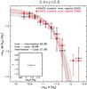 |
Fig. 5 Observed mass functions and Schechter fits for galaxies in different EDisCS cluster regions inside R/R200 = 1. For sake of clarity, only inner (black crosses and solid line) and outer parts (red filled hexagons and dotted line) are plotted. Mass function normalisations, errorbars, labels and the in-set as in Fig. 2. The shape of the mass function is similar in the different regions. |
We now shift our attention to comparing different environments within clusters. As described in Sect. 4, we subdivide clusters into regions with different galaxy clustercentric distances. We first compare in Fig. 4 the mass functions in cluster regions (R/R200 ≤ 1) and the outskirts (R/R200 > 1). Using both ICBS and EDisCS data, K–S tests are unable to detect clearly significant differences (PK − S ≥ 10% in both cases). This is also supported by the Schechter function fit results (see Table 5). For this comparison we have fixed the low-mass-end slope α for the outskirts to be the same as the one obtained for the cluster regions since it is not well constrained. As before, these fits do not describe adequately the bump observed in the EDisCS mass functions at M∗ ~ 1012.3 M⊙, but they work well at lower masses. The fitted parameters indicate that the shape of the mass function is similar in both regions. This is clearly seen for EDisCS, where the statistics are better, but it also seems to be true for the ICBS sample despite the larger statistical uncertainties (Fig. 4).
We next compare three different zones within the cluster virialised regions, the inner (0 ≤ R/R200 < 0.2), intermediate (0.2 ≤ R/R200 < 0.6), and outer (0.6 ≤ R/R200 < 1) parts. Both for ICBS data and EDisCS, the Schechter parameters are compatible within the errors and the K–S test is always inconclusive and thus unable to detect any strong variation with clustercentric distance. To illustrate these results, Fig. 5 shows the mass functions for the inner and outer regions of EDisCS clusters. We do not show the plot for ICBS data since the quality of the statistics is quite low.
In summary, no overall differences are detected between the cluster virialised regions and their outskirts. This agrees with our previous result that the global environment does not alter the shape of the mass distribution since the outskirts of clusters can be considered to be a transition region between the cluster virialised regions and the field, and no differences have been detected between their mass functions. Our results agree with those of von der Linden et al. (2010) derived using SDSS data: excluding BCGs, they found no evidence for mass segregation in clusters since the median mass of cluster galaxies seems to be invariant with cluster radius.
5.4. The mass function of red and blue galaxies does not depend on environment
In previous subsections, we have shown that there appears to be no dependence of the shape of the mass function on the global environment. Our finding is quite surprising because it is known that galaxies located in different environments have different morphological and star formation distributions. The question that arises is whether different galaxy types also follow the same mass distribution.
We subdivide galaxies by colour to separate galaxies with different star formation properties. Following Peng et al. (2010), and after converting to our adopted IMF and the Vega system, galaxies are assigned to the red sequence if their rest-frame colours obey
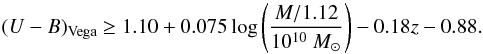 The rest of the galaxies are assigned to the blue cloud.
Figures 6 and 7 present rest-frame (U − B) colours as a function of stellar mass for the ICBS and EDisCS galaxy samples respectively. The cut adopted to separate the red and blue populations is shown. Given the broad redshift range spanned by EDisCS galaxies we divide this sample into four redshift slices. In doing so we avoid the blurring effect of mixing galaxies with very different redshifts and the red sequence and the blue cloud are more easily visible.
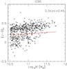 |
Fig. 6 Rest-frame U − B colour vs. stellar mass for the complete ICBS sample. The line separating red and blue galaxies is shown. |
At 0.4 < z < 0.8, contamination from dusty star-forming galaxies can be quite important when selecting red galaxies using only one colour (Wolf et al. 2009). Hence, the stellar mass function of red galaxies is not the stellar mass function of quiescent galaxies only. In EDisCS, the level of dusty star-forming galaxy contamination is ~ 10% for our adopted red galaxy selection (estimated following Brammer et al. 2011). Unfortunately, we cannot make a similar estimate for ICBS given the limited wavelength coverage of our data.
Tables 6 and 7 show the fraction of red and blue galaxies in both samples. As expected, these fractions depend strongly on environment. In the cluster regions, red galaxies dominate, especially at high masses. For M∗ ≥ 1010.5 M⊙, ~ 90% of all galaxies in ICBS are red, and ~60% in EDisCS. This difference shows the expected redshift evolution, If we use the smaller EDisCS mass cut (M∗ ≥ 1010.2 M⊙), we find that for this survey the red fraction is slightly lower (~54%), indicating that blue galaxies have preferentially low masses, as expected. In the ICBS sample, the red fraction reaches a minimum of 41.7% in the cluster outskirts.
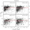 |
Fig. 7 Rest-frame U − B colour vs. stellar mass for the complete EDisCS sample split into four redshift bins. The line separating red and blue galaxies is also shown. |
Fractions of blue and red galaxies in the ICBS sample (0.3 < z < 0.45).
Fractions of blue and red galaxies in the EDisCS sample (0.4 < z < 0.8).
The fraction of red galaxies depends strongly on mass in both samples. Red galaxies dominate the high mass end in any environment. These fractions (see Table 8) are consistent within 1–2σ with the fractions of quiescent galaxies obtained from the number densities given by Brammer et al. (2011) for field galaxies at z ~ 0.613: 50 ± 12% for log M∗/M⊙ = 10.2 − 10.6, 75 ± 19% for log M∗/M⊙ = 10.6 − 11.0, and 92 ± 33% for log M∗/M⊙ = 11.0 − 11.68.
In Fig. 8 we show the mass function of red and blue galaxies using EDisCS data. For M∗ ≥ 1010.2 M⊙, red and blue galaxies have different mass distributions in all the environments considered (clusters, cluster outskirts and groups), Visual inspection and K–S tests indicate these differences are highly significant in all cases. The blue galaxy population tends to contain proportionally more low mass galaxies than the red one. This is particularly evident in clusters (both virialised regions and outskirts). The blue mass function is thus steeper than the red one.
ICBS red and blue galaxies also have clearly different mass functions in the field and outskirts (plots not shown). However, the poor statistics of the ICBS cluster sample prevent the detection of any differences even if present at the same level as in EDisCS clusters. We tested this by using the EDisCS cluster sample to build 1000 Monte-Carlo samples of cluster galaxies with the same numbers and selection criteria as ICBS. In the majority of cases, K–S tests fail to detect significant differences between the mass functions of red and blue galaxies, even though they do exist. Moreover, adopting the higher ICBS mass limit (M∗ ≥ 1010.2 M⊙) for the EDisCS cluster galaxies we still find that red and blue galaxies follow different mass distributions (PK − S = 0.18%). Therefore, the differences are not limited to those found at lower masses.
Red galaxy fractions as a function of mass both in the EDisCS and ICBS samples.
Finally, we compare separately the mass function of blue (Fig. 9) and red (Fig. 10) galaxies in different environments. Visual inspection of the plots and K–S tests provide no indication that the environment affects the mass function of blue and red galaxies. We also derive best-fit Schechter function parameters (Table 9) to the observed mass functions. Since the data lack the necessary number statistics to allow robust estimation of the faint end slope α, we assume fixed values for the red and blue samples separately. For the red galaxies we use α = −0.7 (the same value found by Borch et al. 2006), For the blue galaxies we use α = −1.25, The value used by Borch et al. (2006) (α = −1.45) is too high to describe well our mass functions, so our choice is based on the value obtained by free-fitting the EDisCS mass functions. Due to the high mass limit and the low number statistics, we are unable to find a good fit to the mass function of the blue galaxies in the ICBS clusters. As before, we note that a Schechter fit does not describe well the highest mass end of the EDisCS galaxies.
The analysis of the fit parameters indicates that in all environments red and blue galaxies have comparable values of (within 1–2σ errors). Our findings are in agreement with Borch et al. (2006) and Ilbert et al. (2010). These authors also found that at intermediate redshifts galaxies of different colour show rather similar . Explicitly, at z ~ 0.5, Borch et al. (2006) found that red galaxies have  and blue galaxies 10.93 ± 0.12. Similarly, Ilbert et al. (2010) found that red sequence galaxies have
  and intermediate activity galaxies 10.93 ± 0.03. In summary, we find that galaxies of the same colour are described by mass functions with similar shape and in all environments. This conclusion is particularly robust for the EDisCS survey, given its high number statistics.
6. Discussion
The results from the EDisCS and ICBS samples presented in previous sections are generally in qualitative agreement (or, at the very least, compatible within the uncertainties). Unfortunately, given the different characteristics of both surveys (different redshift ranges and selection criteria), a direct quantitative comparison is not possible. In both surveys, by sampling the mass functions in a broad range of global environments, we are effectively studying galaxies in dark matter haloes with a wide range of masses. Despite this, we find no obvious dependence of the galaxy mass distribution on global environment. Explicitly, galaxies located in clusters, groups, and the field seem to follow mass distributions characterised by similar shapes. This result is surprising and, at some level, perhaps contrary to most expectations.
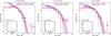 |
Fig. 8 Observed mass functions and Schechter fits for blue and red EDisCS galaxies in clusters (left panel), in cluster outskirts (central panel) and in groups (right panel). Blue filled squares and solid lines correspond to blue galaxies, and red empty triangles and dotted lines to red galaxies. Mass function normalisation, errorbars, labels and in-sets as in Fig. 2. In the in-sets, errorbars represent the 1σ (solid line) and 2σ (dotted line) errors. In clusters, in cluster outskirts, and in groups blue and red galaxies have different mass distributions. |
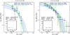 |
Fig. 9 Observed mass function and Schechter function fits for blue galaxies in different environments for the ICBS (left panel) and EDisCS (right panel) samples. Black crosses and solid lines represent the cluster regions, blue filled squares and dotted lines the cluster outskirts, and green empty triangles and dashed lines the groups. The mass distribution of ICBS blue cluster galaxies could not be fitted given the small number of bins. Mass function normalisations, errorbars, labels and in-sets as in Fig. 2. In the in-sets, errorbars represent the 1σ (solid line) and 2σ (dotted line) errors. For blue galaxies, no differences can be detected between the mass functions of galaxies located in clusters, groups, and in the field. |
It will be useful to compare our observational results with theoretical expectations trying to understand whether simulations predict any mass segregation with environment, considering both the initial and evolved halo masses, and their evolution with redshift as a function of environment. This will be the subject of a future paper (Vulcani et al., in prep.). In this section we will concentrate on the empirical results trying to clarify the emerging picture.
6.1. The evolution of the mass function in different environments
In Vulcani et al. (2011) we argued that the evolution observed in clusters is driven by the mass growth of galaxies caused by star formation in both cluster galaxies and, more importantly, in galaxies infalling from the cluster surrounding areas. In that preliminary analysis carried out with inhomogeneous data, we also hypothesized that infalling galaxies could perhaps follow a steeper mass distribution than cluster galaxies. If that were the case, infalling galaxies would contribute more to the intermediate-to-low mass population. However, we found no evidence of any difference between the cluster and field mass functions taken from the literature. In the present work we have analysed the mass functions of galaxies in the field and, most importantly, in the cluster surrounding areas in a self-consistent way. We have thus been able to characterise the mass distribution of galaxies that are supposed to fall into clusters and compare it to the cluster mass function at the same redshift. We have found that for the mass ranges considered (log M∗/M⊙ ≥ 10.5), the mass function is invariant with environment: galaxies located in different environments contain very similar mass distributions. We can thus conclude that the observed evolution of the mass function in clusters (Vulcani et al. 2011) can probably not be explained by galaxies of different masses residing in different environments. This seems to be the case at least for the relatively high galaxy masses studied here. For these galaxies, star formation is the only major process left to explain the observed mass growth, both in clusters and in the field.
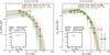 |
Fig. 10 Observed mass function and Schechter function fits for red galaxies in different environments for the ICBS (left panel) and EDisCS (right panel) samples. Black crosses and solid lines represent the cluster regions, red filled squares and dotted lines the cluster outskirts, and green empty triangles and dashed lines the groups. Mass function normalisations, errorbars, labels and in-sets as in Fig. 2. In the in-sets, errorbars represent the 1σ (solid line) and 2σ (dotted line) errors. For red galaxies, no differences can be detected between the mass functions of galaxies located in clusters, groups, and in the field. |
Best-fit Schechter function parameters ( , α, φ∗) for the mass functions of galaxies in different environments and with different colours.
Moreover, by analysing also the field mass function of galaxies in the local universe (Calvi et al., in prep.), we have investigated the evolution of the field mass function from z ~ 0.4 to z ~ 0 and compared this to the evolution found in clusters (Vulcani et al. 2011). Our results show that for log M∗/M⊙ ≥ 10.2 the galaxy stellar mass function evolves in the same way in all environments. In all cases, it becomes steeper with time. Thus, the number of intermediate-mass galaxies grows proportionally at the same rate in clusters and in the field.
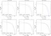 |
Fig. 11 Schechter fits for the blue (blue dotted lines) and red (red dashed lines) galaxies in the ICBS (upper panels) and EDisCS (lower panels) samples in clusters (left panels), the outskirts (central panels) and groups (right panel for EDisCS) and the field (right panel for ICBS). Black vertical dashed lines represent the range in stellar mass probed by these surveys. The curves are not normalised. The blue ICBS cluster mass function is omitted due to poor number statistics. |
Our findings are quite surprising since it is well known that galaxies in different environments and with different stellar masses have different star formation properties and are subject to different physical processes. We expected that the processes responsible for suppressing or halting star formation would be different in clusters and in the field, resulting in different mass growth rates and timescales in different environments. What we find instead is that at the redshifts considered most of the galaxy mass appears to have already been assembled, and that environment-dependent processes have had no significant influence on galaxy mass.
6.2. The blue and red mass functions
In Sect. 5.4 we found that in all environments red and blue galaxies have different mass functions: blue galaxies have steeper mass functions than red ones (Fig. 8). However, we also found that, separately, blue and red galaxies have very similar mass function in all environments (see Figs. 9 and 10). Additionally, the fraction of red and blue galaxies strongly depends on environment: red galaxies dominate the cluster regions while blue galaxies are found mostly in the field. It is therefore quite surprising that the total mass function is almost always the same in all environments.
Figure 11 shows the Schechter functions fitted to the mass functions of galaxies in different environments for colour-selected galaxy samples (see Tables 5 and 9). The fits are used to extrapolate towards lower masses. No additional normalisation has been applied. This figure clearly shows that in all environments blue galaxies dominate in number the mass functions at low masses. Hence, the shape of the total mass function at low masses is regulated by the shape of the blue mass functions. Since the mass functions of blue galaxies have similar α values, the similarity of the total mass functions in the different environments is explained (at least for masses < ). In addition, the similarity of for red and blue galaxies in clusters, groups and the field makes the high mass end of the mass functions similar in all environments.
6.3. Global and local environment
In Vulcani et al. (2012), we analysed specifically the dependence of the mass function on local density, using collectively the WINGS, PM2GC, ICBS, and EDisCS samples. We found that both in the local and distant universe, in clusters and in the field, local density plays an important role in driving the mass distribution. In general, lower density regions host proportionally a larger number of low-mass galaxies than higher density ones. In the field, local density regulates the shape of the mass function for low and high galaxy masses. The situation in clusters is slightly different: local density seems to be important only when we reach relatively low masses (log M∗/M⊙ ≤ 10.1 in WINGS and log M∗/M⊙ ≤ 10.4 in EDisCS). The local density seems to have no significant effect for more massive samples.
In the same study we also found that not only the shape of the mass function is different, but also the highest mass reached: the most massive galaxies are located only the highest density regions, and they are clearly absent in the the lowest densities studied (this is often called mass segregation).
Combining the results of Vulcani et al. (2012) with those of this paper we find that galaxy samples with comparable mass selection limits have mass distributions that vary with local density but not with global environment. In other words, global and local environment appear to influence the shape of the mass functions in very different ways. While the global environment seems to have little effect, local density is clearly important in determining the most fundamental of all galaxy properties, its mass. Clearly, the global and local environments are linked to different physical processes. Their distinct effect on the mass function needs to be understood in order to understand the drivers of galaxy formation and transformation.
6.4. Some caveats
Obviously, the results presented in this paper are only valid for galaxies in the mass ranges covered by our samples. We have no information for masses below log M∗/M⊙ ≃ 10.2 in clusters and groups, and log M∗/M⊙ ≃ 10.5 in the field. At lower masses the situation could well be very different, and deeper surveys are needed to establish the role of the environment for low-mass galaxies.
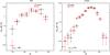 |
Fig. A.1 Luminosity functions in different environments. Left panel: ICBS cluster regions (black crosses) and field (red filled squares). Right panel: EDisCS clusters (black crosses) and groups (red filled squares). In each panel, luminosity functions are normalised using the total integrated luminosity. At the bottom of each panel, the K–S probabilities are given. Significant differences are evident between the luminosity functions in different environments. |
Nevertheless, the mass limits we have adopted are relatively low, so our study is not only relevant to massive galaxies. For instance, the EDisCS mass limit (M∗ ~ 1.6 × 10¹⁰ M⊙) is lower than the critical mass proposed by Kauffmann et al. (2003) separating low-z galaxies in two distinct populations with different stellar population ages, surface mass densities, concentrations, and star formation rates (3 × 10¹⁰ M⊙).
The lack of evidence suggesting a dependence of the mass function on global environment could also be partly due to small number statistics, at least in some cases. Although most of our results seem reasonably reliable, in particular those confirmed in both galaxy samples and those with high statistical significance (e.g., those derived for EDisCS), larger samples would still be desirable. A larger spectroscopic sample of field galaxies would allow, for instance, a better assessment of whether truly isolated galaxies still follow the same mass distribution.
Using photo-z selection for EDisCS galaxies is also not ideal. The level of contamination, even if reasonably low (see e.g. Halliday et al. 2004; Milvang-Jensen et al. 2008), may conceivably still have some effect. Larger spectroscopic surveys would therefore help to confirm (or otherwise) our results.
Our results also depend on the adopted IMF. We implicitly assume that it is universal, regardless of time, environment, and galaxy morphological type. Of course, this may not always be the case. Reports of IMF variation with the star-formation rate (Gunawardhana et al. 2011) or the velocity dispersion of the galaxies (Treu et al. 2009; van Dokkum & Conroy 2011; Thomas et al. 2011; Dutton et al. 2011; Cappellari et al. 2012; Spiniello et al. 2012) have recently appeared in the literature. Obviously, if the IMF is not universal, our results may be quite different since the stellar mass estimates could change in different ways at different galaxy masses. It is fair to say, though, that it would require quite a contrived variation of the IMF with galaxy mass in order to make intrinsically-different mass functions appear the same in all global environments.
7. Conclusions
In this paper we have analysed the shape of the stellar mass function for galaxies in different environments: clusters, groups, and the field. We have used two mass-limited samples covering different redshift ranges, ICBS (0.3 ≤ z ≤ 0.45) and EDisCS (0.4 ≤ z ≤ 0.8). The stellar mass ranges considered are M∗ ≥ 1010.5 M⊙ for ICBS and M∗ ≥ 1010.2 M⊙ for EDisCS. Our main results are:
-
Galaxies in clusters (R ≤ R200), groups, and the field seem to follow similar mass distributions. We find no statistical evidence suggesting a dependence of the shape of the galaxy stellar mass function on global environment at z = 0.3–0.8.
-
By comparing of the ICBS mass functions with mass functions in the local universe (Vulcani et al. 2011 for cluster galaxies and Calvi et al., in prep., for field ones), we find that the evolution of the shape of the mass function from z ~ 0.4 to z ~ 0.07 is the same in the field and in clusters, and hence independent of the global environment. However, the amount of growth with time of the mass function is higher for low-mass galaxies than for massive ones.
-
Galaxies inhabiting the virialised regions of clusters at various clustercentric distances have very similar mass functions. This is also the case for galaxies inside and outside R200.
-
Red and blue galaxies in clusters, groups and the field have different mass functions. However, When comparing the mass functions separately for red and blue galaxies in different environments, no differences are detected.
In summary, we find that the global environment does not seem to have a prominent role in shaping galaxy stellar mass functions. In contrast, the local environment does seem to have significant influence in determining the galaxy mass distribution (Vulcani et al. 2012). This suggests that the most fundamental of all galaxy properties, its mass, is not very dependent on the mass of the halo it inhabits, but it does depend on local scale processes. Global and local environments are clearly linked to different physical processes. Understanding their distinct roles in altering galaxy properties is important in order to understand the drivers of galaxy formation and evolution.
These data are the combination of Bundy et al. (2005) and Bundy et al. (2006) (Bundy, priv. comm.).
The remaining 9% of the relevant galaxies have no mass estimates due to bad photometry or colours.
R200 is defined as the radius delimiting a sphere with interior mean density 200 times the critical density of the universe at that redshift, and is commonly used as an approximation of the cluster virial radius. The R200 values for our structures are computed from the velocity dispersions using the formula
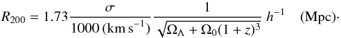
For field samples, we computed the errors given by cosmic variance by estimating the differences between the field mass function and the mass functions obtained using each field separately. Similarly, for clusters we computed the errors due to cluster to cluster variance by comparing the mass functions of each cluster separately.
For EDisCS, we also computed the best-fit Schechter (1976) parameters using the STY (Sandage et al. 1979) method (see, e.g., Marchesini et al. 2009) which is an unbinned maximum likelihood method. In this case the parameters are compatible within 2σ. We do not adopt this method throughout the entire paper because it is not trivial to take into account the ICBS completeness weights.
In agreement with the results of Sect. 5.1, the cut-off masses of low-z mass functions also seem to be different in different environments.
The specific way in which passive and star-forming galaxies are selected strongly affects their measured fractions. Therefore, comparisons between different studies need to be taken with care. Note also that Brammer et al. (2011) study field galaxies in a redshift range slightly higher than the ICBS one.
Acknowledgments
We thank the anonymous referee for her/his detailed and careful comments and suggestions which helped us to improve the manuscript. We thank Lucia Pozzetti for providing the z-COSMOS data for the field mass functions and useful discussion. We also thank Micol Bolzonella for her suggestions. B.V. and B.M.P. acknowledge financial support from ASI contract I/016/07/0 and ASI-INAF I/009/10/0. B.V. also acknowledges financial support from the Fondazione Ing. Aldo Gini. G.D.L. acknowledges financial support from the European Research Council under the European Community’s Seventh Framework Programme (FP7/2007-2013)/ERC grant agreement No. 202781.
References
- Adami, C., Biviano, A., & Mazure, A. 1998, A&A, 331, 439 [NASA ADS] [Google Scholar]
- Aragón-Salamanca, A., Baugh, C. M., & Kauffmann, G. 1998, MNRAS, 297, 427 [NASA ADS] [CrossRef] [Google Scholar]
- Baldry, I. K., Glazebrook, K., Brinkmann, J., et al. 2004, ApJ, 600, 681 [NASA ADS] [CrossRef] [Google Scholar]
- Baldry, I. K., Balogh, M. L., Bower, R. G., et al. 2006, MNRAS, 373, 469 [NASA ADS] [CrossRef] [Google Scholar]
- Baldry, I. K., Glazebrook, K., & Driver, S. P. 2008, MNRAS, 388, 945 [NASA ADS] [Google Scholar]
- Baldry, I. K., Driver, S. P., Loveday, J., et al. 2012, MNRAS, 421, 621 [NASA ADS] [Google Scholar]
- Balogh, M., Navarro, J., & Morris, S. 2000, gfe..conf, [Google Scholar]
- Balogh, M. L., Christlein, D., Zabludoff, A. I., & Zaritsky, D. 2001, ApJ, 557, 117 [NASA ADS] [CrossRef] [Google Scholar]
- Beers, T. C., Flynn, K., & Gebhardt, K. 1990, AJ, 100, 32 [NASA ADS] [CrossRef] [Google Scholar]
- Bekki, K. 2009, MNRAS, 399, 2221 [NASA ADS] [CrossRef] [Google Scholar]
- Bell, E. F., & de Jong, R. S. 2001, ApJ, 550, 212 [NASA ADS] [CrossRef] [Google Scholar]
- Bell, E. F., McIntosh, D. H., Katz, N., & Weinberg, M. D. 2003, ApJS, 149, 289 [NASA ADS] [CrossRef] [Google Scholar]
- Bell, E. F., Wolf, C., Meisenheimer, K., et al. 2004, ApJ, 608, 752 [NASA ADS] [CrossRef] [Google Scholar]
- Blanton, M. R., & Roweis, S. 2007, AJ, 133, 734 [NASA ADS] [CrossRef] [Google Scholar]
- Bolzonella, M., Miralles, J.-M., & Pelló, R. 2000, A&A, 363, 476 [NASA ADS] [Google Scholar]
- Bolzonella, M., Kovač, K., Pozzetti, L., et al. 2010, A&A, 524, A76 [NASA ADS] [CrossRef] [EDP Sciences] [Google Scholar]
- Borch, A., Meisenheimer, K., Bell, E. F., et al. 2006, A&A, 453, 869 [NASA ADS] [CrossRef] [EDP Sciences] [Google Scholar]
- Boselli, A., & Gavazzi, G. 2006, PASP, 118, 517 [NASA ADS] [CrossRef] [Google Scholar]
- Brammer, G. B., Whitaker, K. E., van Dokkum, P. G., et al. 2011, ApJ, 739, 24 [NASA ADS] [CrossRef] [Google Scholar]
- Brunner, R. J., & Lubin, L. M. 2000, AJ, 120, 2851 [NASA ADS] [CrossRef] [Google Scholar]
- Bundy, K., Ellis, R. S., Conselice, C. J., et al. 2005, BAAS, 37, 1235 [NASA ADS] [Google Scholar]
- Bundy, K., Ellis, R. S., Conselice, C. J., et al. 2006, ApJ, 651, 120 [NASA ADS] [CrossRef] [Google Scholar]
- Byrd, G., & Valtonen, M. 1990, ApJ, 350, 89 [NASA ADS] [CrossRef] [Google Scholar]
- Calvi, R., Poggianti, B. M., & Vulcani, B., 2011, MNRAS, 416, 727 [NASA ADS] [Google Scholar]
- Cappellari, M., McDermid, R. M., Alatalo, K., et al. 2012, Nature, 484, 485 [NASA ADS] [CrossRef] [Google Scholar]
- Caputi, K. I., Cirasuolo, M., Dunlop, J. S., et al. 2011, MNRAS, 413, 162 [NASA ADS] [CrossRef] [Google Scholar]
- Conroy, C., White, M., & Gunn, J. E. 2010, ApJ, 708, 58 [NASA ADS] [CrossRef] [Google Scholar]
- De Lucia, G., Poggianti, B. M., Aragón-Salamanca, A., et al. 2004, ApJ, 610, L77 [NASA ADS] [CrossRef] [Google Scholar]
- De Lucia, G., Poggianti, B. M., Aragón-Salamanca, A., et al. 2007, MNRAS, 374, 809 [NASA ADS] [CrossRef] [Google Scholar]
- Dekel, G., Farberovich, V., Fleurov, V., & Soffer, A. 2009 [arXiv:0911.1537] [Google Scholar]
- Desai, V., Dalcanton, J. J., Aragón-Salamanca, A., et al. 2007, ApJ, 660, 1151 [NASA ADS] [CrossRef] [Google Scholar]
- Dressler, A., Oemler, A., Jr.,Poggianti, B. M., et al. 2004, ApJ, 617, 867 [NASA ADS] [CrossRef] [Google Scholar]
- Driver, S. P., Allen, P. D., Graham, A. W., et al. 2006, MNRAS, 368, 414 [NASA ADS] [CrossRef] [Google Scholar]
- Drory, N., & Fisher, D. B. 2007, ApJ, 664, 640 [NASA ADS] [CrossRef] [Google Scholar]
- Drory, N., Salvato, M., Gabasch, A., et al. 2005, ApJ, 619, L131 [NASA ADS] [CrossRef] [Google Scholar]
- Drory, N., Bundy, K., Leauthaud, A., et al. 2009, ApJ, 707, 1595 [NASA ADS] [CrossRef] [Google Scholar]
- Dutton, A. A., Conroy, C., van den Bosch, F. C., et al. 2011, MNRAS, 416, 322 [NASA ADS] [Google Scholar]
- Elsner, F., Feulner, G., & Hopp, U. 2008, A&A, 477, 503 [NASA ADS] [CrossRef] [EDP Sciences] [Google Scholar]
- Fasano, G., Marmo, C., Varela, J., et al. 2006, A&A, 445, 805 [NASA ADS] [CrossRef] [EDP Sciences] [Google Scholar]
- Fasano, G., Bettoni, D., Ascaso, B., et al. 2010, MNRAS, 404, 1490 [NASA ADS] [Google Scholar]
- Fontana, A., Pozzetti, L., Donnarumma, I., et al. 2004, A&A, 424, 23 [NASA ADS] [CrossRef] [EDP Sciences] [Google Scholar]
- Fontana, A., Salimbeni, S., Grazian, A., et al. 2006, A&A, 459, 745 [NASA ADS] [CrossRef] [EDP Sciences] [Google Scholar]
- Gehrels, N. 1986, ApJ, 303, 336 [NASA ADS] [CrossRef] [Google Scholar]
- Gladders, M. D., & Yee, H. K. C. 2000, AJ, 120, 2148 [NASA ADS] [CrossRef] [Google Scholar]
- Gonzalez, A. H., Zaritsky, D., Dalcanton, J. J., & Nelson, A. 2001, ApJS, 137, 117 [NASA ADS] [CrossRef] [Google Scholar]
- González, V., Labbé, I., Bouwens, R. J., et al. 2011, ApJ, 735, L34 [NASA ADS] [CrossRef] [Google Scholar]
- Guo, Y., McIntosh, D. H., Mo, H. J., et al. 2009, MNRAS, 398, 1129 [NASA ADS] [CrossRef] [Google Scholar]
- Gunawardhana, M. L. P., Hopkins, A. M., Sharp, R. G., et al. 2011, MNRAS, 415, 1647 [NASA ADS] [CrossRef] [Google Scholar]
- Gunn, J. E., & Gott, J. R., III 1972, ApJ, 176, 1 [NASA ADS] [CrossRef] [Google Scholar]
- Gwyn, S. D. J., & Hartwick, F. D. A. 2005, AJ, 130, 1337 [NASA ADS] [CrossRef] [Google Scholar]
- Halliday, C., Milvang-Jensen, B., Poirier, S., et al. 2004, A&A, 427, 397 [NASA ADS] [CrossRef] [EDP Sciences] [Google Scholar]
- Holden, B. P., Franx, M., Illingworth, G. D., et al. 2009, ApJ, 693, 617 [NASA ADS] [CrossRef] [Google Scholar]
- Huchra, J. P., & Geller, M. J. 1982, ApJ, 257, 423 [NASA ADS] [CrossRef] [Google Scholar]
- Kajisawa, M., Ichikawa, T., Tanaka, I., et al. 2009, ApJ, 702, 1393 [NASA ADS] [CrossRef] [Google Scholar]
- Kauffmann, G., Heckman, T. M., White, S. D. M., et al. 2003, MNRAS, 341, 54 [Google Scholar]
- Kovač, K., Lilly, S. J., Knobel, C., et al. 2010, ApJ, 718, 86 [NASA ADS] [CrossRef] [Google Scholar]
- Kroupa, P. 2001, MNRAS, 322, 231 [NASA ADS] [CrossRef] [Google Scholar]
- Ilbert, O., Salvato, M., Le Floc’h, E., et al. 2010, ApJ, 709, 644 [NASA ADS] [CrossRef] [Google Scholar]
- Iovino, A., Cucciati, O., Scodeggio, M., et al. 2010, A&A, 509, A40 [NASA ADS] [CrossRef] [EDP Sciences] [Google Scholar]
- Larson, R. B., Tinsley, B. M., & Caldwell, C. N. 1980, ApJ, 237, 692 [NASA ADS] [CrossRef] [Google Scholar]
- Marchesini, D., van Dokkum, P. G., Förster Schreiber, N. M., et al. 2009, ApJ, 701, 1765 [NASA ADS] [CrossRef] [Google Scholar]
- Mercurio, A., Haines, C. P., Merluzzi, P., et al. 2010, jena.conf, [Google Scholar]
- Mihos, J. C., & Hernquist, L. 1996, ApJ, 464, 641 [NASA ADS] [CrossRef] [Google Scholar]
- Milvang-Jensen, B., Noll, S., Halliday, C., et al. 2008, A&A, 482, 419 [NASA ADS] [CrossRef] [EDP Sciences] [Google Scholar]
- Mo, H. J., & White, S. D. M. 1996, MNRAS, 282, 347 [NASA ADS] [CrossRef] [Google Scholar]
- Moore, B., Katz, N., Lake, G., Dressler, A., & Oemler, A. 1996, Nature, 379, 613 [NASA ADS] [CrossRef] [Google Scholar]
- Mortlock, A., Conselice, C. J., Bluck, A. F. L., et al. 2011, MNRAS, 413, 2845 [Google Scholar]
- Moster, B. P., Somerville, R. S., Maulbetsch, C., et al. 2010, ApJ, 710, 903 [NASA ADS] [CrossRef] [Google Scholar]
- Muldrew, S. I., Croton, D. J., Skibba, R. A., et al. 2012, MNRAS, 419, 2670 [NASA ADS] [CrossRef] [Google Scholar]
- Muzzin, A., Marchesini, D., van Dokkum, P. G., et al. 2009, ApJ, 701, 1839 [NASA ADS] [CrossRef] [Google Scholar]
- Oemler, et al. 2012a, submitted [Google Scholar]
- Oemler, et al. 2012b, submitted [Google Scholar]
- Pasquali, A., Leroy, A., Rix, H.-W., et al. 2008, ApJ, 687, 1004 [NASA ADS] [CrossRef] [Google Scholar]
- Pasquali, A., van den Bosch, F. C., Mo, H. J., et al. 2009, MNRAS, 394, 38 [NASA ADS] [CrossRef] [Google Scholar]
- Peng, Y.-j., Lilly, S. J., Kovač, K., et al. 2010, ApJ, 721, 193 [NASA ADS] [CrossRef] [Google Scholar]
- Pelló, R., Rudnick, G., De Lucia, G., et al. 2009, A&A, 508, 1173 [NASA ADS] [CrossRef] [EDP Sciences] [Google Scholar]
- Poggianti, B. M., von der Linden, A., De Lucia, G., et al. 2006, ApJ, 642, 188 [NASA ADS] [CrossRef] [Google Scholar]
- Poggianti, B. M., Desai, V., Finn, R., et al. 2008, ApJ, 684, 888 [NASA ADS] [CrossRef] [Google Scholar]
- Pozzetti, L., Bolzonella, M., Lamareille, F., et al. 2007, A&A, 474, 443 [NASA ADS] [CrossRef] [EDP Sciences] [Google Scholar]
- Pozzetti, L., Bolzonella, M., Zucca, E., et al. 2010, A&A, 523, A13 [NASA ADS] [CrossRef] [EDP Sciences] [Google Scholar]
- Rudnick, G., Franx, M., Rix, H.-W., et al. 2001, AJ, 122, 2205 [NASA ADS] [CrossRef] [Google Scholar]
- Rudnick, G., Rix, H.-W., Franx, M., et al. 2003, ApJ, 599, 847 [NASA ADS] [CrossRef] [Google Scholar]
- Rudnick, G., Labbé, I., Förster Schreiber, N. M., et al. 2006, ApJ, 650, 624 [NASA ADS] [CrossRef] [Google Scholar]
- Rudnick, G., von der Linden, A., Pelló, R., et al. 2009, ApJ, 700, 1559 [NASA ADS] [CrossRef] [Google Scholar]
- Salpeter, E. E. 1955, ApJ, 121, 161 [Google Scholar]
- Sandage, A., Tammann, G. A., & Yahil, A. 1979, ApJ, 232, 352 [NASA ADS] [CrossRef] [EDP Sciences] [Google Scholar]
- Schechter, P. 1976, ApJ, 203, 297 [Google Scholar]
- Sheth, R. K., & Tormen, G. 2002, MNRAS, 329, 61 [NASA ADS] [CrossRef] [Google Scholar]
- Schawinski, K., Virani, S., Simmons, B., et al. 2009, ApJ, 692, L19 [NASA ADS] [CrossRef] [Google Scholar]
- Spiniello, C., Trager, S. C., Koopmans, L. V. E., & Chen, Y. P. 2012, ApJ, 753, L32 [NASA ADS] [CrossRef] [Google Scholar]
- Taylor, E. N., Franx, M., van Dokkum, P. G., et al. 2009, ApJS, 183, 295 [NASA ADS] [CrossRef] [Google Scholar]
- Thomas, D., Maraston, C., Schawinski, K., Sarzi, M., & Silk, J. 2010, MNRAS, 404, 1775 [NASA ADS] [Google Scholar]
- Thomas, J., Saglia, R. P., Bender, R., et al. 2011, MNRAS, 415, 545 [NASA ADS] [CrossRef] [Google Scholar]
- Treu, T., Gavazzi, R., Gorecki, A., et al. 2009, ApJ, 690, 670 [NASA ADS] [CrossRef] [Google Scholar]
- van den Bosch, F. C., Aquino, D., Yang, X., et al. 2008, MNRAS, 387, 79 [Google Scholar]
- von der Linden, A., Wild, V., Kauffmann, G., White, S. D. M., & Weinmann, S. 2010, MNRAS, 404, 1231 [NASA ADS] [Google Scholar]
- van Dokkum, P. G., & Conroy, C. 2011, ApJ, 735, L13 [NASA ADS] [CrossRef] [Google Scholar]
- Vulcani, B., Poggianti, B. M., Finn, R. A., et al. 2010, ApJ, 710, L1 [NASA ADS] [CrossRef] [Google Scholar]
- Vulcani, B., Poggianti, B. M., Aragón-Salamanca, A., et al. 2011, MNRAS, 412, 246 [NASA ADS] [CrossRef] [Google Scholar]
- Vulcani, B., Poggianti, B. M., Fasano, G., et al. 2012, MNRAS, 420, 1481 [NASA ADS] [CrossRef] [Google Scholar]
- Weinmann, S. M., van den Bosch, F. C., Yang, X., & Mo, H. J. 2006, MNRAS, 366, 2 [NASA ADS] [CrossRef] [Google Scholar]
- Whiley, I. M., Aragón-Salamanca, A., De Lucia, G., et al. 2008, MNRAS, 387, 1253 [NASA ADS] [CrossRef] [Google Scholar]
- White, S. D. M., Clowe, D. I., Simard, L., et al. 2005, A&A, 444, 365 [NASA ADS] [CrossRef] [EDP Sciences] [Google Scholar]
- Wild, V., Kauffmann, G., Heckman, T., et al. 2007, MNRAS, 381, 543 [NASA ADS] [CrossRef] [Google Scholar]
- Wolf, C., Aragón-Salamanca, A., Balogh, M., et al. 2009, MNRAS, 393, 1302 [NASA ADS] [CrossRef] [Google Scholar]
Appendix A: Is the mass function simply a mirror of the luminosity function?
Using exactly the same samples as in Sect. 5.1, in this Appendix we build the corresponding luminosity functions to test whether luminosity and mass functions yield equivalent information and results in terms of their environmental differences. We use the absolute magnitudes MV derived in Sects. 3.1 and 3.2 for both ICBS and EDisCS.
In parallel with the mass functions, in each magnitude bin we sum all galaxies belonging to the environment under consideration to obtain the total number of galaxies. The width of each magnitude bin corresponds to 0.4 dex in luminosity. As for the mass functions, histograms are normalised using the total integrated luminosity down to the relevant limits.
For the ICBS survey (left panel of Fig. A.1), we compare cluster regions and the field. The two distributions are different: in clusters the number of more luminous galaxies is proportionally higher than in the field. A K–S test supports this visual impression giving a probability of ~1.4% for both distributions being similar.
In EDisCS (right panel of Fig. A.1), we compare the cluster regions with groups. Again, both from a visual inspection and from a K–S test (PK − S ~ 2.5%), we conclude that the two distributions are different. Groups seem to have a higher number of more luminous galaxies than clusters.
Therefore, using both ICBS and EDisCS data, the luminosity functions of galaxies in different global environments seem statistically different, while the mass functions are indistinguishable (see Sect. 5.1). This shows that studying the luminosity function does not give direct information on the mass function. Galaxies have different colours and mass-to-light ratios and therefore stellar masses do not scale from luminosities by a constant factor.
All Tables
Definitions adopted to characterise the different environments for ICBS (upper panel) and EDisCS (bottom panel).
Number of galaxies in each environment above the stellar mass completeness limits.
Best-fit Schechter function parameters (, α, φ∗) for the mass functions of galaxies in different environments and with different colours.
All Figures
|
Fig. 1 ICBS: redshift distribution in the four fields observed by the survey: RCS0221, RCS1102, SDSS0845, and SDSS1500. The cluster regions ( ± 3σ from cluster redshift) are also indicated (vertical dotted lines). |
| In the text | |
|
Fig. 2 Observed mass functions and Schechter (1976) function fits for galaxies in the different environments. Left panel: ICBS cluster regions (black crosses and solid line) and field (blue empty stars and dotted line). Right panel: EDisCS clusters (black crosses and solid line) and groups (red filled hexagons and dotted line). Mass functions are normalised using the total integrated stellar mass above the mass completeness limits. Errorbars on the x-axis represent the width of the bin. Errorbars on the y-axis are computed combining the Poissonian errors (Gehrels 1986) and the uncertainties due to cosmic variance and cluster-to-cluster variations. Shaded area represent 1σ errors on the Schechter fits. The labels at the top show both the observed and completeness-weighted galaxy numbers for ICBS, while for EDisCS only observed numbers are given. The K–S probabilities are also shown as percentages. The bottom left in-sets in each panel show the M∗ and α Schechter fit parameters with 1σ errors. No significant differences are evident between the galaxy stellar mass distributions in different environments. For ICBS, similar results are also obtained comparing the cluster regions and the non-cluster regions (plot not shown). |
| In the text | |
|
Fig. 3 Comparison between the mass function in clusters and in the field at different redshifts. At low-z, red filled squares: PM2GC (general field); cyan empty squares: Baldry et al. (2008) (general field); blue empty triangles: WINGS (clusters). At intermediate-z, black crosses: ICBS (field); black skeleton triangles: ICBS (clusters). At higher-z: magenta skeleton stars: Pozzetti et al. (2010) (field); green filled triangles EDisCS (clusters). Mass functions are normalised using the total integrated stellar mass in the range 11.2 < log M∗/M⊙ < 11.7 (the last bin in the ICBS). Errorbars and in-set as in Fig. 2. The evolution of the shape of the mass function seems not to depend on environment, being similar in clusters and in the field. However, in all cases the amount of growth as a function of cosmic time is different at the low- and high-mass ends. |
| In the text | |
|
Fig. 4 Observed mass functions and corresponding Schechter function fits for galaxies at different clustercentric distances (R/R200 ≤ 1 and R/R200 > 1) for the ICBS survey (left panel) and EDisCS (right panel). Black crosses and solid lines represent cluster regions, and red empty stars and dotted lines the cluster outskirts. Mass function normalisations, errorbars, labels and in-sets are as in Fig. 2. In both panels, no statistical differences are detected between the mass functions of galaxies located at different clustercentric distances. |
| In the text | |
|
Fig. 5 Observed mass functions and Schechter fits for galaxies in different EDisCS cluster regions inside R/R200 = 1. For sake of clarity, only inner (black crosses and solid line) and outer parts (red filled hexagons and dotted line) are plotted. Mass function normalisations, errorbars, labels and the in-set as in Fig. 2. The shape of the mass function is similar in the different regions. |
| In the text | |
|
Fig. 6 Rest-frame U − B colour vs. stellar mass for the complete ICBS sample. The line separating red and blue galaxies is shown. |
| In the text | |
|
Fig. 7 Rest-frame U − B colour vs. stellar mass for the complete EDisCS sample split into four redshift bins. The line separating red and blue galaxies is also shown. |
| In the text | |
|
Fig. 8 Observed mass functions and Schechter fits for blue and red EDisCS galaxies in clusters (left panel), in cluster outskirts (central panel) and in groups (right panel). Blue filled squares and solid lines correspond to blue galaxies, and red empty triangles and dotted lines to red galaxies. Mass function normalisation, errorbars, labels and in-sets as in Fig. 2. In the in-sets, errorbars represent the 1σ (solid line) and 2σ (dotted line) errors. In clusters, in cluster outskirts, and in groups blue and red galaxies have different mass distributions. |
| In the text | |
|
Fig. 9 Observed mass function and Schechter function fits for blue galaxies in different environments for the ICBS (left panel) and EDisCS (right panel) samples. Black crosses and solid lines represent the cluster regions, blue filled squares and dotted lines the cluster outskirts, and green empty triangles and dashed lines the groups. The mass distribution of ICBS blue cluster galaxies could not be fitted given the small number of bins. Mass function normalisations, errorbars, labels and in-sets as in Fig. 2. In the in-sets, errorbars represent the 1σ (solid line) and 2σ (dotted line) errors. For blue galaxies, no differences can be detected between the mass functions of galaxies located in clusters, groups, and in the field. |
| In the text | |
|
Fig. 10 Observed mass function and Schechter function fits for red galaxies in different environments for the ICBS (left panel) and EDisCS (right panel) samples. Black crosses and solid lines represent the cluster regions, red filled squares and dotted lines the cluster outskirts, and green empty triangles and dashed lines the groups. Mass function normalisations, errorbars, labels and in-sets as in Fig. 2. In the in-sets, errorbars represent the 1σ (solid line) and 2σ (dotted line) errors. For red galaxies, no differences can be detected between the mass functions of galaxies located in clusters, groups, and in the field. |
| In the text | |
|
Fig. 11 Schechter fits for the blue (blue dotted lines) and red (red dashed lines) galaxies in the ICBS (upper panels) and EDisCS (lower panels) samples in clusters (left panels), the outskirts (central panels) and groups (right panel for EDisCS) and the field (right panel for ICBS). Black vertical dashed lines represent the range in stellar mass probed by these surveys. The curves are not normalised. The blue ICBS cluster mass function is omitted due to poor number statistics. |
| In the text | |
|
Fig. A.1 Luminosity functions in different environments. Left panel: ICBS cluster regions (black crosses) and field (red filled squares). Right panel: EDisCS clusters (black crosses) and groups (red filled squares). In each panel, luminosity functions are normalised using the total integrated luminosity. At the bottom of each panel, the K–S probabilities are given. Significant differences are evident between the luminosity functions in different environments. |
| In the text | |
Current usage metrics show cumulative count of Article Views (full-text article views including HTML views, PDF and ePub downloads, according to the available data) and Abstracts Views on Vision4Press platform.
Data correspond to usage on the plateform after 2015. The current usage metrics is available 48-96 hours after online publication and is updated daily on week days.
Initial download of the metrics may take a while.