| Issue |
A&A
Volume 548, December 2012
|
|
|---|---|---|
| Article Number | A39 | |
| Number of page(s) | 11 | |
| Section | Interstellar and circumstellar matter | |
| DOI | https://doi.org/10.1051/0004-6361/201220067 | |
| Published online | 16 November 2012 | |
Synthetic observations of first hydrostatic cores in collapsing low-mass dense cores
II. Simulated ALMA dust emission maps
1
Laboratoire de radioastronomie, UMR 8112 du CNRS, École Normale Supérieure
et Observatoire de Paris,
24 rue Lhomond,
75231
Paris Cedex 05,
France
e-mail: This email address is being protected from spambots. You need JavaScript enabled to view it.
2
ESO, Karl Schwarzschild Strasse 2, 85748
Garching bei München,
Germany
3
Max-Planck-Institut für Astronomie, Königstuhl 17, 69117
Heidelberg,
Germany
Received: 20 July 2012
Accepted: 2 October 2012
Abstract
Context. First hydrostatic cores are predicted by theories of star formation, but their existence has never been demonstrated convincingly by (sub)millimeter observations. Furthermore, the multiplicity in the early phases of the star formation process is poorly constrained.
Aims. The purpose of this paper is twofold. First, we seek to provide predictions for ALMA dust continuum emission maps from early Class 0 objects. Second, we show to what extent ALMA will be able to probe the fragmentation scale in these objects.
Methods. Following our companion paper, we post-processed three state-of-the-art radiation-magneto-hydrodynamic 3D adaptive mesh refinement calculations to compute the emanating dust emission maps. We then produced synthetic ALMA observations of the dust thermal continuum from first hydrostatic cores.
Results. We present the first synthetic ALMA observations of dust continuum emission from the first hydrostatic cores. We analyze the results given by the different bands and configurations and we discuss for which combinations of the two the first hydrostatic cores would most likely be observed. We also show that observing dust continuum emission with ALMA will help in identifying the physical processes occurring within collapsing dense cores. If the magnetic field is playing a role, the emission pattern will show evidence of a pseudo-disk and even of a magnetically driven outflow, which pure hydrodynamical calculations cannot reproduce.
Conclusions. The capabilities of ALMA will enable us to make significant progress towards understanding the fragmentation at the early Class 0 stage and discovering first hydrostatic cores.
Key words: stars: formation / stars: low-mass / magnetohydrodynamics (MHD) / radiative transfer / techniques: interferometric / methods: numerical
© ESO, 2012
1. Introduction
It has been established that most stars form in multiple systems (Duquennoy & Mayor 1991; Janson et al. 2012). This indicates a fragmentation process during star formation, which can be explained by several mechanisms (e.g., Bodenheimer et al. 2000; McKee & Ostriker 2007). The first picture is to consider the interplay between turbulence and gravity within molecular clouds, which can lead to an initial fragmentation prior to the collapse (Hennebelle & Chabrier 2008). In this picture, the stellar initial mass function (IMF) is mainly determined at the dense-core formation stage, and the dense cores undergo collapse without fragmenting into individual objects (e.g., Price & Bate 2007; Hennebelle & Teyssier 2008; Commerçon et al. 2010). On the other hand, fragmentation may also occur during the collapse of molecular clouds (e.g Bate & Bonnell 2005; Bate 2012) or within disks that are formed because of the conservation of angular momentum (e.g., Whitworth & Stamatellos 2006; Commerçon et al. 2008). The fragmentation process thus remains a matter of intense debate; in particular, disk formation and early fragmentation (i.e., during the early phase of the collapse) appear to be critical for better constraining the star formation mechanism (e.g., Li et al. 2011; Joos et al. 2012; Seifried et al. 2012).
The tremendous combined developments of observational and supercomputing capabilities allow study of astrophysical processes on scales that have remained unresolved until today. In particular, strong advances in understanding the star formation process have been achieved during the past ten years. On the one hand, thanks to various (sub)millimeter interferometric facilities (e.g., the IRAM Plateau de Bure Interferometer, PdBI, and the Submillimeter Array, SMA) and to the Spitzer and Herschel space telescopes, much progress has been achieved towards understanding the formation and structure of prestellar dense cores and constraining the evolutionary stages of star-forming regions (e.g., Kennicutt & Evans 2012). On the other hand, numerical models of star formation integrate more and more physical processes. Among the most important ones, magnetic fields and radiative transfer appear to shape the collapse and fragmentation of prestellar dense cores (e.g., Hennebelle & Teyssier 2008; Bate 2009), while their combined feedback dramatically inhibits fragmentation in low- and high-mass collapsing dense cores (Commerçon et al. 2010, 2011b). Unfortunately, there is currently no direct evidence of these mechanisms, since observations are not yet able to probe the fragmentation scale in nearby star-forming regions. While wide ≳5000 AU multiple systems are often detected around the youngest (Class 0) protostars (e.g., Chen et al. 2008; Launhardt et al. 2010), the highest resolution observations so far with synthesized half power beamwidths of 0.3″−1″ (e.g., using the IRAM PdBI or the SMA) show a lack of close ≲2000 AU multiple systems (Maury et al. 2010). However, at a distance of the nearest star-forming regions (e.g., 140 pc for Taurus), this angular resolution only probes linear scales larger than 40–50 AU. To probe smaller scales, Atacama Large Millimeter/Submillimeter Array (ALMA) observations are definitely needed.
First hydrostatic cores (FHSC), i.e., first Larson cores (Larson 1969) are the first protostellar objects formed during the star formation process with typical sizes of a few AU. Although their existence is predicted by theory (e.g., Larson 1969; Masunaga et al. 1998; Tomida et al. 2010b; Commerçon et al. 2011a), there is still no strong observational evidence of such objects, because FHSCs are deeply embedded within collapsing cores, and their lifetimes are relatively short (at most a few thousand years, e.g., Tomida et al. 2010a; Commerçon et al. 2012, hereafter Paper I) compared to the Class 0 phase duration (0.1–0.2 Myr, Evans et al. 2009). Several candidate FHSCs are known (e.g., Belloche et al. 2006; Chen et al. 2010; Pineda et al. 2011; Chen et al. 2012), but none has yet been confirmed. We showed in Paper I that spectral energy distributions (SEDs) of star-forming clumps can help in identifying FHSC candidates, but are not able to assess the physical conditions within the cores and, in particular, the level of fragmentation. For that, high-resolution interferometric imaging is needed. It is also unclear to what extent FHSCs can be distinguished from more evolved very low-luminosity objects (VeLLOs; di Francesco et al. 2007) and second hydrostatic cores (i.e., the protostars).
Summary of the physical structures and FHSC lifetimes found in the three models.
To address this necessity for theoretical predictions of the appearance of early phases of star formation, Krumholz et al. (2007), Semenov et al. (2008), Cossins et al. (2010), and Offner et al. (2012) have presented synthetic ALMA observations of dust continuum or line emission. In this paper, we present the first predictive dust-emission maps of embedded FHSCs as they should be observable with ALMA. This study focusing on dust continuum is considered as a first step towards FHSC characterization in combination with the results of Paper I.
The paper is organized as follows. Section 2 presents the physical models and the method we use to derive synthetic ALMA dust emission maps. Section 3 reports on the results we obtain to select the best ALMA configuration and the best receiver band for observing FHSCs. We discuss the limitation of our work in Sect. 4. Section 5 presents our conclusions and perspectives concerning future work needed to confirm the results obtained as a first step along with dust continuum observations.
2. Method
In this study, we restrict our work to the early stages of the star formation process, i.e., the first collapse and FHSC formation. As mentioned in the introduction, a lot of progress has been made in theory and observations to characterize what we would expect at those early stages. In the following, we combine state-of-the-art tools to produce synthetic ALMA dust emission observations.
2.1. The physical models
We performed 3D full radiation-magneto-hydrodynamic (RMHD) calculations using the adaptive mesh refinement code RAMSES (Teyssier 2002), which integrates the equations of ideal magneto-hydrodynamics (Fromang et al. 2006) and uses the gray flux-limited-diffusion approximation for the radiative transfer (Commerçon et al. 2011c). We used the same RMHD calculations presented in Paper I, which consisted in letting rotating (in solid-body rotation) 1 M⊙ dense cores collapse, with initially uniform temperature, density, and magnetic field. The ratio of the initial thermal and rotational energies to the gravitational energy are α = 0.35 and β = 0.045, respectively. We ran three different models with the same initial conditions except for the initial magnetization, which is parametrized by the mass-to-flux to critical mass-to-flux ratio μ = (M0/Φ)/(M0/Φ)c. The three models are depicted as MU2 model (strong magnetic field, μ = 2), MU10 model (intermediate magnetic field, μ = 10), and MU200 model (quasi-hydro case, μ = 200). These three models are representative of the diversity of FHSCs and of their environments (disk, pseudo-disk, and outflow), which are both predicted by the theory. The different physical structures and FHSC lifetimes found in the three models are summarized in Table 1. In the MU2 model, only one FHSC is formed, surrounded by a pseudo-disk, and an outflow was launched. The MU10 model does not fragment either and results in a system composed of a disk, a pseudo-disk, and an outflow. The MU200 model has classical features of hydrodynamical models, in which relatively large disks (~150 AU) are formed and subsequently fragment. Readers are referred to Paper I for a thorough description of the different models and their limitations. The MU2 and MU10 models are more representative of the observed magnetization level in star-forming regions (i.e., μ ≈ 2−3, Falgarone et al. 2008; Crutcher et al. 2010), even though determining magnetic field strength remains challenging.
In the following, the calculations have been post-processed at the same times as in Fig. 2 of Paper I. These are representative of the characteristics of the three models, i.e., t0 + 0.78 kyr for the MU2 model, t0 + 1.81 kyr for the MU10 model, and t0 + 3.26 kyr for the MU200 model (where t0 corresponds to the FHSCs formation in each model, i.e. 50.4 kyr for MU2, 35.7 kyr for MU10, and 35.4 kyr for MU200).
2.2. Dust emission models with RAMDC-3D
We used the same interface as presented in Paper I, which couples the outputs of the RMHD calculations, which are done within RAMSES, to the 3D radiative transfer code RADMC-3D1. In this interface, we assumed that gas and dust are thermally coupled (Tdust = Tgas), which is a valid approximation given the high density within the dense cores (e.g, Galli et al. 2002). We also assumed that the gas temperature Tgas computed in the RMHD calculations is correct (Commerçon et al. 2011a; Vaytet et al. 2012). We used the low-temperature opacities of Semenov et al. (2003) for a model in which dust is made of homogeneous spheres with a “normal” (Fe/Fe + Mg = 0.3) silicate composition.
Characteristics of the ALMA bands used, denoted B.
The dust thermal continuum emission maps were computed on a square box with physical size Δx = 1300 AU and a resolution δx = 2.54 AU. Since models were assumed to be at a distance D = 150 pc, this translates into an angular extent Δϑ = 8.67″ and an angular resolution δϑ = 0.017″. Four different viewing angles are used in the following: θ = 0° (equatorial plane seen face-on), θ = 45°, θ = 60°, and θ = 90° (edge-on view, perpendicular to the rotational axis). These model dust-emission maps were computed for six ALMA bands (3, 4, 6, 7, 8, and 9), including the four that are in use in the early science stage (see Table 2), over a total bandwidth Δν = 8 GHz centered on the band’s central frequency ν0. This was done by computing a set of ten emission maps, one for each of ten 800 MHz sub-bands, and averaging them. The resulting map gives the mean specific intensity ⟨Iν⟩ of the thermal dust emission over the band, in erg cm-2 s-1 Hz-1 sr-1, and is then converted to a brightness temperature map in K via2
2.3. Producing synthetic ALMA observations
The GILDAS software package3, which has been developed and maintained by IRAM, is primarily intended for reducing and analyzing observational data acquired via the IRAM instruments (single-dish 30-m radiotelescope at Pico Veleta and 6-antenna array at IRAM PdBI). It also includes a full ALMA simulator with up-to-date array configurations4, which was primarily developed to assess the impact of the ALMA compact array (ACA) on the imaging capabilities of ALMA (Pety et al. 2001; Tsutsumi et al. 2004).
To produce synthetic ALMA observations from our dust emission models, maps were converted to the GILDAS data format (GDF) and projected on a fixed sky position (α0,δ0) = (0°, −23°) such that sources transit at the zenith of the array. The field-of-view in each band (see Table 2), given by 1.22λ0/d with d = 12 m the antenna diameter and λ0 the central wavelength of the band, shows that a single pointing suffices to map the emission in all cases.
Characteristics of the full ALMA configurations used, denoted C.
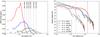 |
Fig. 1 Left: probability density function from the distribution of samples in the u − v plane for the 4 configurations used here (numbers 5, 10, 15, and 20, indicated next to each curve) as a function of u − v radius |

ALMA consists of two subarrays, the fifty 12-m antennas and the twelve 7-m antennas of the ACA. The array operation will consist in constantly moving antennas around, so that no two observations may be obtained with exactly the same configuration. We did not consider the compact array and focused on imaging the cores’ thermal emission with ALMA alone. To keep the number of simulations down to a manageable number, we selected four “typical” configurations (out of the 28 representative configurations implemented in GILDAS), whose properties are listed in Table 3. Since we made one simulation per model, per configuration, per inclination angle, and per band, the total number of simulations is thus 3 × 4 × 4 × 5 = 240. In all cases, model sources are observed for a total integration time of 18 minutes centered on the transit.
The ALMA simulator is a full pipeline, including the deconvolution of dirty images via a CLEAN algorithm (Clark 1980). Outputs can thus be compared directly to input images smoothed to the same resolution, which the simulator also provides.
3. Results
3.1. A necessary compromise
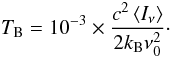
In our models, thermal dust emission at millimeter and submillimeter wavelengths mostly comes from structures that are larger than the FHSC (i.e., from the disk and the pseudo-disk). Nevertheless, to distinguish between different magnetization levels μ, one needs to resolve the fragmentation scale of a few AU. This constraint means that only extended configurations of the array will be able to provide sufficient angular resolution, in the few tens of milliarcsecond range. However, this comes with an increase in the minimum baseline length, so that large-scale emission is lost owing to the central hole in the visibility (Fourier) space, also called u − v plane.
To make this idea more quantitative, Fig. 1 (left) shows the distribution of visibility samples as a function of radius in the u − v plane for the four configurations. Marked on this graph are the baselines duv = cD/(2πν0d) corresponding to a physical size d = 10 AU (roughly equal to the size of fragments in the MU200 models) at a distance D = 150 pc, for the six central frequencies ν0. In the right plot of Fig. 1, we display the power spectra of the face-on input maps at 100 GHz (band 3) and 661 GHz (band 9), with the wavenumber axis k rescaled to match that of the u − v radius in the left hand plot. This is done by noticing that the largest wavenumber in the power spectrum corresponds to the pixel physical size δx.
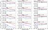 |
Fig. 2 Ratio Fobs/Fmodel of the observed flux to the model flux as a function of frequency, for the three different models (MU2, MU10, and MU200), four array configurations (C = 5,10,15,20), and four inclinations (θ = 0°,45°,60°,90°). Magnetization level decreases from left to right, and inclination angle θ increases from top to bottom. |
The fragmentation in the MU200 model appears as the excess power on intermediate scales compared to MU2 and MU10. This excess is clearly seen for 300 m ≲ duv ≲ 2000 m at 100 GHz, with duv = 2000 m roughly corresponding to the 10 AU scale at 150 pc. As far as the four configurations used here are concerned, this range of baselines is beyond C = 5 and best probed by configurations C = 15 and C = 20. However, both of these configurations have a larger central hole than C = 5 and C = 10, and therefore should lose a larger amount of flux. This flux loss becomes greater at higher frequencies, since duv ∝ 1/ν0 implies a global compression of the sources’ power spectra towards smaller baselines.
For a global view of the emission loss on large scales, Fig. 2 shows the ratio between the observed flux to the model flux as a function of frequency and array configuration. As expected, the most compact configurations (C = 5 and C = 10) allow essentially all of the flux to be recovered in bands 3 to 7. Only in bands 8 and 9 do we see a ~50% drop in the received flux for the non-fragmenting models MU2 and MU10. Figure 2 also confirms that flux loss increases with frequency in configurations 15 and 20, since most (~80%) of the flux is already lost at 144 GHz in configuration 20. Overall, it appears that observing in bands 3 and 4 with configuration 15 may provide the best compromise, as the flux loss is very limited (less than 8%), and according to the left hand plot in Fig. 1, it should be able to resolve the fragmentation scale, at least in band 4.
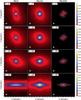 |
Fig. 3 Brightness distribution maps in Jy/beam, output by the ALMA simulator in band B = 3 (100 GHz), and array configuration C = 15. Magnetization level decreases from left to right, and inclination angle θ increases from top to bottom. Contours show the 3σS sensitivity limit in this band, as given by the ALMA Sensitivity Calculator. Here σS = 14.55 μJy. The synthesized beam is shown in the bottom left corner of each plot. For a given θ, color scales are identical across all columns. |
3.2. Emission maps
We show in Fig. 3 to 6 the brightness distribution maps output by the ALMA simulator in bands 3 and 4 for configurations 15 and 20. In each figure, four inclination angles are shown, i.e., θ = 0°,45°,60°, and 90°. Also shown are the sensitivity limits 3σS in these two bands, given by the ALMA Sensitivity Calculator5. The most extended configuration and the highest frequency probe the fragmentation scales best (C = 20, B = 4 in Fig. 6). However, as we discussed above, a significant amount of the flux emanating from the extended emission is lost in configuration 20. On the other hand, the fragmentation scale is barely resolved with C = 15 and B = 3. A better compromise between high-resolution imaging and flux recovering is found using either C = 15 and B = 4 or C = 20 and B = 3. Overall, there is a clear distinction between the two magnetized models (MU2 and MU10) and the quasi-hydro MU200 model. As expected theoretically, as soon as a magnetic field is taken into account, with field strengths in the range of what is actually observed (e.g., Falgarone et al. 2008; Crutcher et al. 2010; Maury et al. 2012), the picture changes dramatically.
Interestingly, many features that directly probe the physical conditions can already be observed with the dust emission (see Table 1). In the MU200 model, the fragmentation is resolved for inclination angles θ < 60°, and only the compact emission of the disk is observed in the edge-on view. In contrast to that, the dust emission is much more extended in the magnetized MU2 and MU10 models, and corresponds to density features that are typical of magnetized collapse: the pseudo-disk and the outflow. In both cases, the most powerful emission comes from the central FHSC (point-like source, yellow area). In the MU10 model, the disk emission is observed (blue regions) for inclination angles θ < 60°, but it remains relatively weak in comparison to the pseudo-disk one. The pseudo-disk emission features are very similar in the MU2 and MU10 models for inclination angles θ < 60°. In the edge-on view (θ = 90°), the emission from the pseudo-disk is clearly observed in the MU2 and MU10 models, and is much more extended than that of the disk in the MU200 model. The pattern of the pseudo-disk observed with C = 20 and B = 4 in the MU2 model may lead to confusion since it has the shape of a flared disk. Additional line emission observations are then needed to distinguish between a disk and a pseudo-disk in that case. Last but not least, the outflow is also observed in the MU10 model in Figs. 3 to 5 with an extent of ~4″ along the polar axis, corresponding to ~300 AU. This is not surprising since the outflow tends to transport more mass in the case of a lower magnetization (Hennebelle & Fromang 2008,and see Fig. 2 in Commerçon et al. 2012).
We investigate thoroughly the effects of noise (thermal and atmospheric phase) and pointing errors on the synthetic observations in Appendix A. The main conclusions drawn from the noise-free case remain unchanged, except that more flux is lost in noisy observations. We refer interested readers to Appendix A.
4. Discussion
One limitation of this work is that we used a unique dust opacity model from Semenov et al. (2003), in which dust grains can grow, so that we do not predict the variation in the dust emission with different dust grain properties. The dust properties (size, composition, and morphology) within dense cores are still very uncertain, but there is nevertheless theoretical and observational evidence of dust grain growth within dense cores (e.g., Ormel et al. 2009; Steinacker et al. 2010). Ormel et al. (2011) compare the dust grain opacities they got from the various grain models of Ormel et al. (2009) with the Ossenkopf & Henning (1994) opacities model and find that the opacity in the submillimeter wavelength range only varies by a factor of a few between all the different models. We also checked that the Semenov et al. (2003) opacities we used are similar to those from the Ossenkopf & Henning (1994) by factors close 1, so that the choice in the opacity will not change the picture. In addition, we show in Paper I (Fig. 4) that the radius at which the optical depth equals unity does not depend strongly on the opacity for (sub)millimeter wavelengths. We thus speculate that our predictions are relatively robust given the small variations in optical depth and in opacity in the (sub)millimeter wavelength range.
The second main limitation comes from our idealized initial and boundary conditions, which do not account for the dense core environment (e.g., eventual mass accretion on the core while it collapses) and initial turbulence, whereas the latter can potentially modify the magnetic braking and thus the fragmentation properties during the collapse (e.g., for higher mass dense cores, Seifried et al. 2012). Turbulence, however, is observed to be sub- to trans-sonic in low-mass dense cores (Goodman et al. 1998; André et al. 2007), so that it will not dramatically change the outcome of the magnetized dense core collapse. In addition, magnetic fields dominate the dynamics and inhibit the fragmentation even more when combined with radiative transfer because of the energy released from the accretion shock at the FHSC border (Commerçon et al. 2010, 2011b). We thus conclude that the three models presented here are representative of the variety of FHSCs that can be formed with various initial conditions.
Finally, all the analysis and the ALMA synthetic map calculations have been done for objects placed at a distance of 150 pc. The best compromise between flux loss and angular resolution may thus be altered for objects at significantly different distances, but the method remains unchanged.
5. Summary and perspectives
We have presented synthetic dust emission maps of FHSCs as they will be observed by the ALMA interferometer, using state-of-the-art radiation-magneto-hydrodynamic models of collapsing dense cores with different levels of magnetic intensity. We post-processed the RMHD calculations performed with the RAMSES code using the 3D radiative transfer code RADMC-3D to produce dust-emission maps. The synthetic observations were then computed using the ALMA simulator within the GILDAS software package.
We showed that ALMA will shed light on the fragmentation process during star formation and will help in distinguishing not only between the different physical conditions, but also between the different models of star formation and fragmentation. The forthcoming facility will yield interferometric observations of FHSC candidates (selected using SED data, see Paper I) in nearby star-forming regions with enough angular resolution to probe the fragmentation scale. We also showed that the intensity of the magnetic field in this early phase of protostellar collapse will also be assessed, since we do see clear morphological differences between the magnetized and non-magnetized models, i.e., pseudo-disk and outflow in the former case versus disk and fragmentation features in the latter case. We stressed that owing to the unprecedented sensitivity and coverage of the instrument, this will be achievable in a very short time (18 min), so that many FHSC candidates may be observed in a single observing run.
Reaching high enough angular resolution to probe the fragmentation scales and limiting the loss of large-scale emission requires a compromise, which is achieved using frequency bands 3 and 4 and the relatively extended configurations 15 and 20. We also investigated the effect of noise on the interferometric observations and showed that in typical conditions (see Fig. A.1), ALMA will still be able to reveal fragmentation. We noted that the effect of atmospheric phase noise can be efficiently reduced using water-vapor radiometers on the ALMA antennas.
We did not discuss the impact of the ALMA Compact Array (ACA) on our simulated observations. Its purpose is to provide measurements for the large-scale emission and improve the wide-field imaging capabilities of ALMA (Pety et al. 2001), but it is not meant to resolve fragmented molecular cores. In our models, this requires a 0.5′′ angular resolution (see e.g., the case B = 3 and C = 15 in Figs. 1 and 3), but the longest baselines accessible to ACA are ~100 m, so that the highest angular resolution available, at the high-frequency end of band 10 (950 GHz), is 0.8′′. However, ACA could help recover some of the lost flux from the disk, pseudo-disk, and outflow.
Our work is currently limited to the dust continuum emission, which cannot provide robust means yet to distinguish between FHSC and second hydrostatic cores and to decide on the nature of VeLLOs. Further work including molecular line emission calculations is thus warranted to better probe the physical conditions (density, temperature, etc.) in observed collapsing cores, for instance to disentangle the disk and the pseudo-disk, which should harbor different line profiles (rotation-dominated versus infall-dominated). Line emission predictions are thus the obvious next step toward characterizing FHSCs.
The factor 10-3 comes from the CGS to SI conversion of the specific intensity, as the ALMA simulator assumes input brightness distributions to be in K.
iram.fr/IRAMFR/GILDAS/
We used release apr11h of GILDAS. The latest releases also contain early science Cycle 1 configurations of the array.
The weather conditions used are that of the first octile, i.e., 0.47 mm of precipitable water vapor above the instrument.
Acknowledgments
We thank the anonymous referee for his/her comments. F.L. wishes to thank Jérôme Pety, Alwyn Wootten, and Ian Heywood for their collaboration in including the final ALMA configurations in the GILDAS simulator. The research of B.C. is supported by postdoctoral fellowships from the CNES and by the French ANR Retour Postdoc program.
References
- André, P., Belloche, A., Motte, F., & Peretto, N. 2007, A&A, 472, 519 [NASA ADS] [CrossRef] [EDP Sciences] [Google Scholar]
- Asayama, S., Kawashima, S., Iwashita, H., et al. 2008, in Ninteenth Int. Symp. on Space Terahertz Technology, ed. W. Wild, 244 [Google Scholar]
- Bate, M. R. 2009, MNRAS, 392, 1363 [NASA ADS] [CrossRef] [Google Scholar]
- Bate, M. R. 2012, MNRAS, 419, 3115 [NASA ADS] [CrossRef] [Google Scholar]
- Bate, M. R., & Bonnell, I. A. 2005, MNRAS, 356, 1201 [NASA ADS] [CrossRef] [Google Scholar]
- Belloche, A., Parise, B., van der Tak, F. F. S., et al. 2006, A&A, 454, L51 [NASA ADS] [CrossRef] [EDP Sciences] [Google Scholar]
- Bodenheimer, P., Burkert, A., Klein, R. I., & Boss, A. P. 2000, in Protostars and Planets IV, eds. V. Mannings, A. P. Boss, & S. S. Russell (Tucson: Univ. Arizona Press), 675 [Google Scholar]
- Chen, X., Bourke, T. L., Launhardt, R., & Henning, T. 2008, ApJ, 686, L107 [NASA ADS] [CrossRef] [Google Scholar]
- Chen, X., Arce, H. G., Zhang, Q., et al. 2010, ApJ, 715, 1344 [Google Scholar]
- Chen, X., Arce, H. G., Dunham, M. M., et al. 2012, ApJ, 751, 89 [NASA ADS] [CrossRef] [Google Scholar]
- Clark, B. G. 1980, A&A, 89, 377 [NASA ADS] [Google Scholar]
- Commerçon, B., Hennebelle, P., Audit, E., Chabrier, G., & Teyssier, R. 2008, A&A, 482, 371 [NASA ADS] [CrossRef] [EDP Sciences] [Google Scholar]
- Commerçon, B., Hennebelle, P., Audit, E., Chabrier, G., & Teyssier, R. 2010, A&A, 510, L3 [NASA ADS] [CrossRef] [EDP Sciences] [Google Scholar]
- Commerçon, B., Audit, E., Chabrier, G., & Chièze, J.-P. 2011a, A&A, 530, A13 [NASA ADS] [CrossRef] [EDP Sciences] [Google Scholar]
- Commerçon, B., Hennebelle, P., & Henning, T. 2011b, ApJ, 742, L9 [NASA ADS] [CrossRef] [Google Scholar]
- Commerçon, B., Teyssier, R., Audit, E., Hennebelle, P., & Chabrier, G. 2011c, A&A, 529, A35 [NASA ADS] [CrossRef] [EDP Sciences] [Google Scholar]
- Commerçon, B., Launhardt, R., Dullemond, C., & Henning, T. 2012, A&A, 545, A98 [NASA ADS] [CrossRef] [EDP Sciences] [Google Scholar]
- Cossins, P., Lodato, G., & Testi, L. 2010, MNRAS, 407, 181 [NASA ADS] [CrossRef] [Google Scholar]
- Crutcher, R. M., Wandelt, B., Heiles, C., Falgarone, E., & Troland, T. H. 2010, ApJ, 725, 466 [NASA ADS] [CrossRef] [Google Scholar]
- di Francesco, J., Evans, II, N. J., Caselli, P., et al. 2007, in Protostars and Planets V, eds. B. Reipurth, D. Jewitt, & K. Keil (Tucson: Univ. Arizona Press), 17 [Google Scholar]
- Duquennoy, A., & Mayor, M. 1991, A&A, 248, 485 [NASA ADS] [Google Scholar]
- Evans, II, N. J., Dunham, M. M., Jørgensen, J. K., et al. 2009, ApJS, 181, 321 [NASA ADS] [CrossRef] [Google Scholar]
- Falgarone, E., Troland, T. H., Crutcher, R. M., & Paubert, G. 2008, A&A, 487, 247 [NASA ADS] [CrossRef] [EDP Sciences] [Google Scholar]
- Fromang, S., Hennebelle, P., & Teyssier, R. 2006, A&A, 457, 371 [NASA ADS] [CrossRef] [EDP Sciences] [Google Scholar]
- Galli, D., Walmsley, M., & Gonçalves, J. 2002, A&A, 394, 275 [NASA ADS] [CrossRef] [EDP Sciences] [Google Scholar]
- Goodman, A. A., Barranco, J. A., Wilner, D. J., & Heyer, M. H. 1998, ApJ, 504, 223 [NASA ADS] [CrossRef] [Google Scholar]
- Hennebelle, P., & Chabrier, G. 2008, ApJ, 684, 395 [NASA ADS] [CrossRef] [Google Scholar]
- Hennebelle, P., & Fromang, S. 2008, A&A, 477, 9 [NASA ADS] [CrossRef] [EDP Sciences] [Google Scholar]
- Hennebelle, P., & Teyssier, R. 2008, A&A, 477, 25 [NASA ADS] [CrossRef] [EDP Sciences] [Google Scholar]
- Janson, M., Hormuth, F., Bergfors, C., et al. 2012, ApJ, 754, 44 [NASA ADS] [CrossRef] [Google Scholar]
- Joos, M., Hennebelle, P., & Ciardi, A. 2012, A&A, 543, A128 [NASA ADS] [CrossRef] [EDP Sciences] [Google Scholar]
- Kennicutt, R. C., & Evans, N. J. 2012, ARA&A, 50, 531 [NASA ADS] [CrossRef] [Google Scholar]
- Krumholz, M. R., Klein, R. I., & McKee, C. F. 2007, ApJ, 665, 478 [NASA ADS] [CrossRef] [Google Scholar]
- Larson, R. B. 1969, MNRAS, 145, 271 [NASA ADS] [CrossRef] [Google Scholar]
- Launhardt, R., Nutter, D., Ward-Thompson, D., et al. 2010, ApJS, 188, 139 [NASA ADS] [CrossRef] [Google Scholar]
- Li, Z.-Y., Krasnopolsky, R., & Shang, H. 2011, ApJ, 738, 180 [NASA ADS] [CrossRef] [Google Scholar]
- Masunaga, H., Miyama, S. M., & Inutsuka, S.-I. 1998, ApJ, 495, 346 [Google Scholar]
- Maury, A. J., André, P., Hennebelle, P., et al. 2010, A&A, 512, A40 [NASA ADS] [CrossRef] [EDP Sciences] [Google Scholar]
- Maury, A. J., Wiesemeyer, H., & Thum, C. 2012, A&A, 544, A69 [NASA ADS] [CrossRef] [EDP Sciences] [Google Scholar]
- McKee, C. F., & Ostriker, E. C. 2007, ARA&A, 45, 565 [NASA ADS] [CrossRef] [Google Scholar]
- Offner, S. S. R., Capodilupo, J., Schnee, S., & Goodman, A. A. 2012, MNRAS, 420, L53 [NASA ADS] [Google Scholar]
- Ormel, C. W., Paszun, D., Dominik, C., & Tielens, A. G. G. M. 2009, A&A, 502, 845 [NASA ADS] [CrossRef] [EDP Sciences] [Google Scholar]
- Ormel, C. W., Min, M., Tielens, A. G. G. M., Dominik, C., & Paszun, D. 2011, A&A, 532, A43 [NASA ADS] [CrossRef] [EDP Sciences] [Google Scholar]
- Ossenkopf, V., & Henning, T. 1994, A&A, 291, 943 [NASA ADS] [Google Scholar]
- Pety, J., Gueth, F., & Guilloteau, S. 2001, in ALMA Memo, 398 [Google Scholar]
- Pineda, J. E., Arce, H. G., Schnee, S., et al. 2011, ApJ, 743, 201 [NASA ADS] [CrossRef] [Google Scholar]
- Price, D. J., & Bate, M. R. 2007, MNRAS, 377, 77 [NASA ADS] [CrossRef] [Google Scholar]
- Seifried, D., Banerjee, R., Pudritz, R. E., & Klessen, R. S. 2012, MNRAS, 423, L40 [Google Scholar]
- Semenov, D., Henning, T., Helling, C., Ilgner, M., & Sedlmayr, E. 2003, A&A, 410, 611 [NASA ADS] [CrossRef] [EDP Sciences] [Google Scholar]
- Semenov, D., Pavlyuchenkov, Y., Henning, T., Wolf, S., & Launhardt, R. 2008, ApJ, 673, L195 [NASA ADS] [CrossRef] [Google Scholar]
- Steinacker, J., Pagani, L., Bacmann, A., & Guieu, S. 2010, A&A, 511, A9 [NASA ADS] [CrossRef] [EDP Sciences] [Google Scholar]
- Teyssier, R. 2002, A&A, 385, 337 [NASA ADS] [CrossRef] [EDP Sciences] [Google Scholar]
- Tomida, K., Machida, M. N., Saigo, K., Tomisaka, K., & Matsumoto, T. 2010a, ApJ, 725, L239 [NASA ADS] [CrossRef] [Google Scholar]
- Tomida, K., Tomisaka, K., Matsumoto, T., et al. 2010b, ApJ, 714, L58 [NASA ADS] [CrossRef] [Google Scholar]
- Tsutsumi, T., Morita, K.-I., Hasegawa, T., & Pety, J. 2004, in ALMA Memo, 488 [Google Scholar]
- Vaytet, N., Audit, E., Chabrier, G., Commerçon, B., & Masson, J. 2012, A&A, 543, A60 [NASA ADS] [CrossRef] [EDP Sciences] [Google Scholar]
- Whitworth, A. P., & Stamatellos, D. 2006, A&A, 458, 817 [NASA ADS] [CrossRef] [EDP Sciences] [Google Scholar]
Appendix A: Noisy observations
The simulations presented in the main body of the paper were performed in the unrealistic case of noiseless observations. To truly assess ALMA’s ability to resolve fragmented cores, an extension of this study to noisy observations is required, taking into account the different causes of noise: pointing errors, thermal noise, and phase noise.
We start with an error-free simulation of the MU200 model viewed face-on (θ = 0°) in band B = 4, with configuration C = 20. All parameters are identical to those of the general set of simulations, but we add zero-spacing with a single-dish observation, so that in this case all of the flux is recovered (0.1090 Jy) instead of 96% of it (0.1046 Jy) with ALMA alone.
The following errors, whose results are summarized in Table A.1, may then be added, separately or simultaneously, to the simulated observations :
-
▸
0.6′′ random pointing errors σα, which correspond to ~15% of the primary beam width at 144 GHz. They may be applied to the ALMA antennas alone or to both ALMA and single-dish measurements.
-
▸
Thermal noise σT. In band 4, the ALMA Sensitivity Calculator suggests using the 6th octile for the atmospheric conditions, which corresponds to 2.75 mm of precipitable water vapor and a zenith opacity τ = 0.057. The band 4 receiver noise is set to T144 = 40 K following Asayama et al. (2008). Regarding the single-dish measurements, we use a system temperature Tsys = 100 K. The simulator allows for setting none, either, or both ALMA and single-dish thermal noises.
-
▸
Atmospheric phase noise σφ. The ALMA simulator allows for a turbulent atmospheric screen to pass over the interferometer, distorting the waveplanes and causing phase errors. This 2D phase screen is characterized by a second-order structure function that is the combination of three power laws in three spatial ranges, scaled so that the rms phase difference for a 300-m baseline takes a specific value. In our case, we chose this value to be either 30° or 45° (Pety et al. 2001). Situated at an altitude z = 1000 m, the screen passes over the instrument at a windspeed w = 10 m s-1. Calibration, which is done every 26 s using a calibrator 2 degrees away from the source perpendicularly to the wind direction, may include the use of water vapor radiometers (WVR), which directly measure the amount of precipitable water vapor along the line of sight in the atmosphere above each antenna.
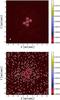 |
Fig. A.1 Brightness distribution maps, in Jy/beam, for two cases considered in section A. The top plot shows the case of an error-free observation at 144 GHz with ALMA in configuration C = 20, combined with single-dish. The bottom plot shows the case of an observation with the same combination of instruments, but with 0.6′′ pointing errors on all antennas, thermal noise as described in the text, and uncorrected atmospheric phase noise with a 45° rms phase difference on 300-m baselines. Contours on both plots correspond to the 3σS sensitivity limit given by the ALMA Sensitivity Calculator, where σS = 17.41 μJy for the typical atmospheric conditions in band B = 4. |
Effect of the different noise types.
Table A.1 gives simulation results associated to the various noise situations considered: fluxes S in the output (deconvolved) maps and median fidelities F0.3, F1, F3, and F10 on pixels whose intensities in the model image are higher than 0.3%, 1%, 3%, and 10% of the peak, respectively. The fidelity is basically the inverse of the relative error between the output map and the model (Pety et al. 2001), so that the higher the fidelity, the better the reconstruction. What is apparent is that atmospheric phase noise has the strongest impact on the reconstruction process, with a third of the flux being lost in the worst-case scenario and fidelities dropping to a few (30%–50% relative error on the output maps). The use of WVR is a definite plus in this situation, because relative errors then drop to a little over 10%. However, even in the worst possible situation considered here, and without WVR correction, ALMA still is able to uncover fragmentation, since Fig. A.1 shows that all five fragments in the model map are fully observed above the noise level in these typical conditions.
All Tables
All Figures
|
Fig. 1 Left: probability density function from the distribution of samples in the u − v plane for the 4 configurations used here (numbers 5, 10, 15, and 20, indicated next to each curve) as a function of u − v radius |
| In the text | |
|
Fig. 2 Ratio Fobs/Fmodel of the observed flux to the model flux as a function of frequency, for the three different models (MU2, MU10, and MU200), four array configurations (C = 5,10,15,20), and four inclinations (θ = 0°,45°,60°,90°). Magnetization level decreases from left to right, and inclination angle θ increases from top to bottom. |
| In the text | |
|
Fig. 3 Brightness distribution maps in Jy/beam, output by the ALMA simulator in band B = 3 (100 GHz), and array configuration C = 15. Magnetization level decreases from left to right, and inclination angle θ increases from top to bottom. Contours show the 3σS sensitivity limit in this band, as given by the ALMA Sensitivity Calculator. Here σS = 14.55 μJy. The synthesized beam is shown in the bottom left corner of each plot. For a given θ, color scales are identical across all columns. |
| In the text | |
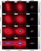 |
Fig. 4 Same as Fig. 3 but for B = 4 and C = 15. Here, σS = 16.05 μJy. |
| In the text | |
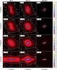 |
Fig. 5 Same as Fig. 3 but for B = 3 and C = 20. Here, σS = 14.55 μJy. |
| In the text | |
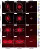 |
Fig. 6 Same as Fig. 3 but for B = 4 and C = 20. Here, σS = 16.05 μJy. |
| In the text | |
|
Fig. A.1 Brightness distribution maps, in Jy/beam, for two cases considered in section A. The top plot shows the case of an error-free observation at 144 GHz with ALMA in configuration C = 20, combined with single-dish. The bottom plot shows the case of an observation with the same combination of instruments, but with 0.6′′ pointing errors on all antennas, thermal noise as described in the text, and uncorrected atmospheric phase noise with a 45° rms phase difference on 300-m baselines. Contours on both plots correspond to the 3σS sensitivity limit given by the ALMA Sensitivity Calculator, where σS = 17.41 μJy for the typical atmospheric conditions in band B = 4. |
| In the text | |
Current usage metrics show cumulative count of Article Views (full-text article views including HTML views, PDF and ePub downloads, according to the available data) and Abstracts Views on Vision4Press platform.
Data correspond to usage on the plateform after 2015. The current usage metrics is available 48-96 hours after online publication and is updated daily on week days.
Initial download of the metrics may take a while.