| Issue |
A&A
Volume 540, April 2012
|
|
|---|---|---|
| Article Number | A1 | |
| Number of page(s) | 19 | |
| Section | Interstellar and circumstellar matter | |
| DOI | https://doi.org/10.1051/0004-6361/201117623 | |
| Published online | 13 March 2012 | |
Variations on a theme – the evolution of hydrocarbon solids⋆
I. Compositional and spectral modelling – the eRCN and DG models
1 Institut d’Astrophysique Spatiale, CNRS, IAS UMR8617, 91405 Orsay, France
2 Université Paris Sud, IAS UMR 8617, 91405 Orsay, France
e-mail: This email address is being protected from spambots. You need JavaScript enabled to view it.
Received: 4 July 2011
Accepted: 30 October 2011
Abstract
Context. The compositional properties of hydrogenated amorphous carbons are known to evolve in response to the local conditions.
Aims. We present a model for low-temperature, amorphous hydrocarbon solids, based on the microphysical properties of random and defected networks of carbon and hydrogen atoms, that can be used to study and predict the evolution of their properties in the interstellar medium.
Methods. We adopt an adaptable and prescriptive approach to model these materials, which is based on a random covalent network (RCN) model, extended here to a full compositional derivation (the eRCN model), and a defective graphite (DG) model for the hydrogen poorer materials where the eRCN model is no longer valid.
Results. We provide simple expressions that enable the determination of the structural, infrared and spectral properties of amorphous hydrocarbon grains as a function of the hydrogen atomic fraction, XH. Structural annealing, resulting from hydrogen atom loss, results in a transition from H-rich, aliphatic-rich to H-poor, aromatic-rich materials.
Conclusions. The model predicts changes in the optical properties of hydrogenated amorphous carbon dust in response to the likely UV photon-driven and/or thermal annealing processes resulting, principally, from the radiation field in the environment. We show how this dust component will evolve, compositionally and structurally in the interstellar medium in response to the local conditions.
Key words: dust, extinction / ISM: general
Appendices A and B are available in electronic form at http://www.aanda.org
© ESO, 2012
1. Introduction
In this paper we will refer to an amorphous hydrocarbon particle as any finite-sized, macroscopically-structured (i.e. a contiguous network of atoms), solid-state material consisting solely of carbon and hydrogen atoms. There is now a wealth of laboratory data on such materials (e.g., Smith 1984; Robertson 1986; Angus & Hayman 1988; Robertson & O’Reilly 1987; Mennella et al. 1995; Scott et al. 1997; Grishko & Duley 2000; Ferrari & Robertson 2004; Duley et al. 2005b; Hu & Duley 2008a) and also a number of theoretical models which interpret their inherent structures (e.g., Robertson 1986; Robertson & O’Reilly 1987; Angus & Jansen 1988; Robertson 1988; Tamor & Wu 1990; Jones 1990; Duley 1995; Dadswell & Duley 1997; Duley et al. 2005a) and it is upon these data and models that we shall rely in constructing a model for the evolution of hydrocarbon grains in the interstellar medium (ISM).
It has long been known that laboratory hydrocarbon solids darken upon exposure to ultraviolet (UV) light and to heating (e.g., Iida et al. 1985; Smith 1984), and that this photo-darkening of the materials is accompanied by a decrease in the band gap or optical gap energy, Eg. It is this property that is at the heart of the inherent variability of the optical properties of such solid materials, and that is of prime interest in the context of the applicability of these properties in unravelling the histories of hydrocarbon grains in the ISM (e.g., Duley 1996).
The evolution of hydrocarbon materials is therefore of key interest for the study of interstellar dust properties because it appears that graphite is no longer a tenable candidate to explain the dust properties associated with carbon-rich interstellar dust (e.g., Dartois et al. 2004b, 2005; Serra Díaz-Cano & Jones 2008; Compiègne et al. 2011). Amorphous hydrocarbons, however, do appear to be a widespread component of interstellar dust in galaxies (e.g., Dartois et al. 2004a). These materials are consistent with the observed infrared absorption bands (e.g., Dartois et al. 2004b; Dartois & Muñoz-Caro 2007) and show temperature-dependent luminescence (e.g., Robertson 1986) consistent with the observed interstellar luminescence in the red, the so-called extended red emission (ERE, Duley et al. 1997; Duley 2001; Dartois et al. 2005; Godard & Dartois 2010) and with the likely irradiation effects and the associated aliphatic to aromatic transformation in the ISM (e.g., Jones 1990; Dartois et al. 2004a,b; Pino et al. 2008; Mennella 2008; Godard et al. 2011), in circumstellar regions (e.g., Goto et al. 2003, 2007; Sloan et al. 2007; Pino et al. 2008), in interplanetary dust particles (IDPs, Muñoz Caro et al. 2006) and solar system organics (Dalle Ore et al. 2011).
The work presented here was conceived with the application of the random covalent network (RCN) theory for the structure of amorphous hydrocarbon materials (Phillips 1979; Döhler et al. 1980; Thorpe 1983; Angus & Jansen 1988; Jones 1990) to the astrophysical context (Jones 1990) and this series of follow-up papers has therefore been some 21 years in gestation.
In this paper we study the compositional, structural and spectral properties of amorphous hydrocarbon materials and apply this to the nature of low-temperature particles in the ISM.
The paper is organised as follows: in Sects. 2 and 3 we present the eRCN and defective graphite (DG) models for the structural evolution of hydrogenated amorphous carbons and their associated spectra, in Sect. 4 we discuss the astrophysical implications for the evolution of carbonaceous dust in the ISM, in Sect. 5 we summarise the model predictions, in Sect. 6 we discuss the limitations of the eRCN/DG models, and in Sect. 7 we present out conclusions.
In the ensuing, associated papers we study the compositional and wavelength-dependent optical properties of amorphous hydrocarbons within the astrophysical context (Jones 2012a, hereafter Paper II) and the rôle of size effects on those optical properties (Jones 2012b, hereafter Paper III).
2. Structural models for amorphous hydrocarbons
Hydrocarbon materials span the entire compositional range between the ordered diamond-like solids and graphite-like solids (CHn, where n ≈ 0) and organic polymers (CHn, where n ≈ 2), but it is the amorphous hydrocarbon materials that exist between these various forms that are of most interest here (CHn, where 0 ≤ n ≤ 2). This is because amorphous hydrocarbons exhibit properties that can change in response to their irradiation and thermal histories (e.g., Jones 1990).
The crucial parameters that define the structures (i.e. the short-range order) of amorphous hydrocarbon materials are the carbon atom bonding, in particular the ratio of the sp3 and sp2 fractions, and the hydrogen content (Robertson 1986; Robertson & O’Reilly 1987; Angus & Jansen 1988; Jones 1990). Of particular relevance is the way in which the sp3 and sp2 carbon atoms cluster, as indeed they must if they are to preserve the required atomic configurations (Angus & Jansen 1988; Jones 1990). Hydrocarbon solids therefore consist of domains of diamond-like or aliphatic (sp3 bonded) and graphite-like or aromatic (sp2 bonded) carbon intimately connected in networks that lack any long-range order but that are bridged by aliphatic and olefinic structures. The domains may consist of only a few to a few tens of atoms and contain both C and H atoms. At the short-range or atomic level there is some regularity in the networks due to the geometrical constraints imposed by the bonding of the carbon atoms as a function of their hybridisation state i.e. sp3 or sp2, over the long-range there is no significant order.
In order to understand the structures of hydrocarbon materials a particularly useful set of models have been the RCN theories (Phillips 1979; Döhler et al. 1980; Thorpe 1983; Angus & Jansen 1988; Jones 1990). These use the average nearest-neighbour bonding environment to constrain a macroscopic RCN of carbon and hydrogen atoms. The network is completely constrained when the number of constraints per atom (related to the coordination number) is equal to the number of mechanical degrees of freedom (the dimensionality, Phillips 1979). Within a network the formation of bonds leads to increased stability, however, in a random network directed bonds lead to strain energy due to distortions in the bond lengths and angles. The optimal network is one that just balances these two effects.
In the following sections we summarise the salient points of the RCN theories and extend the model to more complex compositions.
2.1. The basic random covalent network model
In order to aid the reader, we here summarise the essential elements of the RCN formalism, which is described in detail elsewhere (Phillips 1979; Döhler et al. 1980; Thorpe 1983; Angus & Jansen 1988; Jones 1990).
If in a network m is the coordination number of a given atom (1 for hydrogen, and 2, 3 and 4 for sp1, sp2 and sp3 carbon atoms, respectively) then the number of constraints for a given atomic site, Ncon, in a three-dimensional network, where the bonding is dominated by nearest neighbour, directed valence bonds is, as given by Döhler et al. (1980), 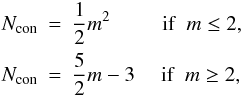 (1)and for a completely constrained network consisting of several types of atom of coordination number i and atomic fraction xi,
 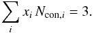 (2)Hydrocarbon materials can be considered to consist primarily of only hydrogen atoms, and sp2 and sp3 carbon atoms (Robertson 1986; Jones 1990). Any sp1 hybridised carbon atoms are of very low abundance in these materials and are, for simplicity, ignored in the RCN model. In this case two equations then relate the atom fractions for each component, x1 (H), x3 (sp2) and x4 (sp3), respectively, i.e.,
 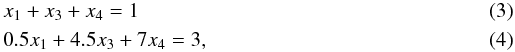 \arraycolsep1.75ptand with some simple algebra we then have that
 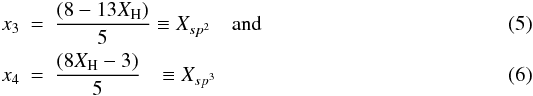 where XH is the atomic fraction of hydrogen ( ≡ x1). The ratio, R, of the sp3 and sp2 atom fractions and the average coordination number,
  , is then, following Angus & Jansen (1988),
  \arraycolsep1.75ptwhere we now replace the fundamental quantities x3 and x4, the sp2 and sp3 carbon atom fractions, respectively, by the more explicit symbols Xsp2 and Xsp3. The average carbon atom coordination number is obtained by considering only the Xsp2 and Xsp3 fractions in Eq. (8) and then re-normalising to the carbon atom fraction (1 − XH), i.e.,
  (9)From Eq. (7) we can see that for sp3 bonding only, i.e. setting Xsp2 = 0, we have XH = 8/13 = 0.615. For hydrogen concentrations greater than 0.615 the number of bonds is insufficient to use up all the degrees of freedom and the network will be “under-constrained”. For sp2 bonding only we can similarly set Xsp3 = 0 and in this case we have XH = 3/8 = 0.375. For hydrogen concentrations less than 0.375 the network would be “over-constrained”. In general, if the number of constraints per atom is greater than the number of dimensions then the network will re-construct in some way and small clusters violating this simple RCN model would be expected to appear. From the limits of the validity of Eq. (7) we see that these RCNs can therefore only exist over the hydrogen content range 0.38 ≲ XH ≲ 0.62.
Strictly, the above description is only valid for systems where the triply coordinated sp2 carbon atoms are randomly distributed. However, sp2 sites must pair up into, at least, ethylenic units, i.e., > C=C < , with a coordination number of 4 (Angus & Jansen 1988) and these structures are observed in the IR spectra of a-C:H (Dischler et al. 1983a,b). The equations governing the RCN network with paired sp2 sites, analogous to Eqs. (3) to (9), are then,  and in this case the above expressions are valid for 0.17 ≲ XH ≲ 0.62. This range, derived using a rather simple model, is in excellent agreement with laboratory data (Angus & Jansen 1988) and indicates the compositions for which completely constrained hydrocarbon networks can exist. In Fig. 1 we show R as a function of XH for the models presented in this section and calculated using Eqs. ((7), dotted line) and ((14), short dash-dotted line).
For RCN networks consisting of H atoms, sp3 carbon atoms and C2sp2 carbon ethylenic ( > C=C < ) groups, and where 0.17 ≲ XH ≲ 0.62, the range of values for the mean atomic coordination number, , given by Eq. (15), is  . For an H-poor, aromatic-rich structure the limiting lower limit must be close to three, while the upper limit should approach that for a (CH2)n polymer, i.e.,
  , which is clearly consistent with the H-rich limit of 2.15 derived here. The mean carbon atom coordination,
  , given by Eq. (16), is equivalently
  , which reproduces the expected values, i.e., 3.0 for sp2-only and 4.0 for sp3-only structures.
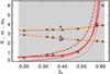 |
Fig. 1 Carbon atom ratio R as a function of XH. Dotted line: basic RCN model (Eq. (7)), short-dashed-dotted line: C2sp2 clusters (Eq. (14)), long-dashed line: all sp2 carbon atoms in C6 aromatic clusters (Eq. (35)) and solid line: multi-C6 ring aromatic clusters (Eq. (40)) and methyl groups (Eq. (52)). The upper and flatter solid lines show the mean atomic coordination number, |


Duley (1995) extended the RCN model to include sp3 C6H10 “diamond-like” clusters with four aliphatic CH2 groups and two tertiary CH groups. We note, however, that the smallest aliphatic cluster of this type is actually the adamantane-like cluster C10H16, which actually contains six aliphatic CH2 groups and four tertiary CH groups.
2.2. The extended RCN model (eRCN)
With the aim of simplifying our further, and following, extensions to the basic RCN model(s), and in order to facilitate the algebraic manipulations, we now parameterise Eqs. (4) and (11) to:  (17)and then, following some simple algebra, derive generalised expressions for the sp3 and sp2 carbon atom fractions (Xsp3 and Xsp2), their ratio R ≡ Xsp2/Xsp3, and the average atomic coordination number, , i.e.,
 ![Mathematical equation: \begin{eqnarray} &&X_{sp^3} = \frac{(8X_{\rm H}-3)}{5} = \frac{(b-a)X_{\rm H}-(b-3)}{(c-b)} = \frac{R(1-X_{\rm H})}{(1+R)}, \label{gen_Xsp3_abc} \\ &&X_{sp^2} = \frac{(8-13X_{\rm H})}{5} = \frac{(c-3)-(c-a)X_{\rm H}}{(c-b)} = \frac{(1-X_{\rm H})}{(1+R)}, \label{gen_Xsp2_abc} \\ &&R = \frac{(b-a)X_{\rm H}-(b-3)}{(c-3)-(c-a)X_{\rm H}}, \label{gen_R_abc} \\ &&\bar{m} = X_{\rm H} + 3X_{sp^2} + 4X_{sp^3}, \notag\\ &&\ \ \ \ = X_{\rm H} + 3\left[ \frac{(c-3)-(c-a)X_{\rm H}}{(c-b)} \right] + 4\left[ \frac{(b-a)X_{\rm H}-(b-3)}{(c-b)} \right], \notag\\ &&\ \ \ \ = X_{\rm H} + \frac{3(1-X_{\rm H})}{(1+R)} + \frac{4R(1-X_{\rm H})}{(1+R)}, \notag\\ &&\ \ \ \ = \frac{(3-2X_{\rm H})+(4-3X_{\rm H})R}{(1+R)}\cdot \label{gen_m_abc} \end{eqnarray}](/articles/aa/full_html/2012/04/aa17623-11/aa17623-11-eq54.png) In the above expressions, and in many of those that follow, the factor (1 − XH) often appears; this is simply the total carbon atomic fraction, i.e., (1 − XH) ≡ (Xsp2 + Xsp3) ≡ XC. However, given that the key parameter for RCN, and the following eRCN, models is XH, the substitution of XC for (1 − XH) is not particularly useful or informative and we chose not to make it here.
In the above expressions, and in many of those that follow, the factor (1 − XH) often appears; this is simply the total carbon atomic fraction, i.e., (1 − XH) ≡ (Xsp2 + Xsp3) ≡ XC. However, given that the key parameter for RCN, and the following eRCN, models is XH, the substitution of XC for (1 − XH) is not particularly useful or informative and we chose not to make it here.
It is clear that hydrogen atoms do not contribute to the connectivity of a network and, if we neglect their contribution and re-normalise to the total number of carbon atoms, we derive the general formula for the mean carbon atom coordination number,  , for the carbon framework, i.e.,
 ![Mathematical equation: \begin{eqnarray} \bar{m}_{\rm C} &\,=\,& 3\left(\frac{X_{sp^2}}{1-X_{\rm H}}\right) + 4\left(\frac{X_{sp^3}}{1-X_{\rm H}}\right) = \frac{(3+4R)}{(1+R)}, \notag\\ &=& 3 \left[ \frac{(c-3)-(c-a)X_{\rm H}}{(c-b)(1-X_{\rm H})} \right] + 4 \left[ \frac{(b-a)X_{\rm H}-(b-3)}{(c-b)(1-X_{\rm H})} \right]\cdot \label{gen_mC_abc} \end{eqnarray}](/articles/aa/full_html/2012/04/aa17623-11/aa17623-11-eq57.png) (22)In most RCN systems we find that
(22)In most RCN systems we find that  and c = 7 and we can therefore further simplify the above expressions to,
 ![Mathematical equation: \begin{eqnarray} &&X_{sp^3} = \frac{(2b-1)X_{\rm H}-(2b-6)}{2(7-b)}, \\ &&X_{sp^2} = \frac{(8-13X_{\rm H})}{2(7-b)}, \\ &&R = \frac{(2b-1)X_{\rm H}-(2b-6)}{(8-13 X_{\rm H})}, \label{gen_R_b} \\ &&\bar{m} = \frac{2(7-b)X_{\rm H} + 3[8-13X_{\rm H}] + 4[(2b-1)X_{\rm H}-(2b-6)]}{2(7-b)}, \notag\\ &&\ \ \ \ = \frac{(48-8b)-(29-6b)X_{\rm H}}{2(7-b)}, \label{gen_m_b} \\ &&\bar{m}_{\rm C} = \frac{3(8-13X_{\rm H}) + 4[(2b-1)X_{\rm H}-(2b-6)]}{2(7-b)}, \notag\\ &&\ \ \ \ \ \ = \frac{(48-8b)-(43-8b)X_{\rm H}}{2(7-b)(1-X_{\rm H})}\cdot \label{gen_mC_b} \end{eqnarray}](/articles/aa/full_html/2012/04/aa17623-11/aa17623-11-eq60.png) In our calculations we always use the appropriate expressions for a, b and c, substituted into Eqs. (18) to (22), so as to avoid any algebraic errors that may have crept into the derivation of the more explicit equations presented in the following sections.
In our calculations we always use the appropriate expressions for a, b and c, substituted into Eqs. (18) to (22), so as to avoid any algebraic errors that may have crept into the derivation of the more explicit equations presented in the following sections.
2.2.1. Aromatic structures in eRCNs
The RCN formalism was further extended to the more realistic case where the sp2 carbon atoms are allowed to cluster into C6 aromatic ring units Jones (1990), which is consistent with the fact that even-numbered C atom clusters are more stable and therefore favoured (Robertson 1986). This introduces six-fold coordination sites, X6, with Ncon = 12. The X6 sites exhibit only short-range order and their inclusion in the RCN scheme is therefore valid. The equations for atomic conservation and the summed atomic constraints then become 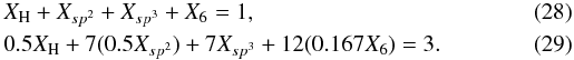 If f is the fraction of the sp2 carbon atoms in the C6 units then X6 ≡ fXsp2 and the two above equations become
 ![Mathematical equation: \begin{eqnarray} &&X_{\rm H} + (1-f)X_{sp^2} + X_{sp^3} + fX_{sp^2} = X_{\rm H} + X_{sp^2} + X_{sp^3} = 1, \\ &&0.5X_{\rm H} + 7 [0.5 (1-f) X_{sp^2}] + 12(0.167 f X_{sp^2}) + 7X_{sp^3} = 3, \notag\\ &&0.5X_{\rm H} + 7 [0.5 (1-f) + 2 f ] X_{sp^2} + 7X_{sp^3} = 3. \end{eqnarray}](/articles/aa/full_html/2012/04/aa17623-11/aa17623-11-eq69.png) The equations for R and are then, for a = 0.5, b = 7 [0.5(1 − f) + 2f] = 0.5(7 − 3f) an c = 7,
The equations for R and are then, for a = 0.5, b = 7 [0.5(1 − f) + 2f] = 0.5(7 − 3f) an c = 7, 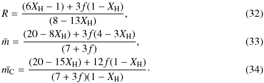 These equations reduce to those given previously when f = 0. The case for f = 1, i.e. all the sp2 carbon atoms in C6 rings, gives
  which leads to a good fit to the laboratory data for amorphous hydrocarbons for low values of XH (see Fig. 1). However, at higher hydrogen contents the fit is less good because too much order is introduced into the network due to the “forced” insertion of unrealistic aromatic ring structures into a predominantly aliphatic network.
The RCN model can be further adapted to allow for the presence of multi-C6 ring aromatic domains of sp2 carbon atoms, i.e., the introduction of polycyclic aromatics (Jones 1990). This formalism can be summarised in the following set of equations for the atomic conservation, the summed atomic constraints, the ratio R and the average atomic coordination numbers, respectively, ![Mathematical equation: \begin{eqnarray} &&X_{\rm H} + X_{sp^2} + X_{sp^3} = 1, \label{RvsXH_fit3_frac} \\ &&0.5X_{\rm H} + \{ 7 [0.5(1-f)] + Zf \} X_{sp^2} + 7X_{sp^3} = 3. \end{eqnarray}](/articles/aa/full_html/2012/04/aa17623-11/aa17623-11-eq77.png) In the interests of space-saving in the following, we define an aromatic carbon component parameter Yf = (7 − 2Z)f. Here we now have a = 0.5, b = (7 [0.5(1 − f)] + Zf) = 0.5 [7 − (7 − 2Z)f] = 0.5(7 − Yf) and c = 7 and then
In the interests of space-saving in the following, we define an aromatic carbon component parameter Yf = (7 − 2Z)f. Here we now have a = 0.5, b = (7 [0.5(1 − f)] + Zf) = 0.5 [7 − (7 − 2Z)f] = 0.5(7 − Yf) and c = 7 and then 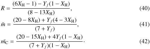 Here Z is a function of the number of six-fold rings, NR, in the polycyclic aromatic clusters and is the number of constraints per carbon atom for the given cluster, i.e.,
 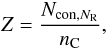 (43)where nC is the number of carbon atoms per aromatic cluster. The relevant expressions for Z for linear and compact aromatic clusters are given in Appendix A. As above, f is the fraction of sp2 carbon atoms in the aromatic clusters or domains and is an empirically-derived function of XH. Here we have adopted an expression, which differs from that of Jones (1990), in that we use a smooth transition from the maximum value of f (fmax) at low XH to f ≈ 0 at high XH using
 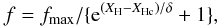 (44)where we take fmax = 0.6 as the maximum fraction of sp2 carbon atoms in the aromatic clusters, XHc = 0.33 as a critical hydrogen atom fraction and δ = 0.07, which parameterises the steepness of the transition between high and low f. It appears that our results are not particularly sensitive to the exact form of f, provided that the shape of the transition is physically “reasonable”.
If the simplifying assumption is again made that f = 1 then it is an easy matter to calculate R as a function of XH for a wide range of aromatic clusters (PAH-like species). Rather surprisingly when this is done the results do not differ significantly from the single six-fold ring case, even for 4–5 ring linear and compact aromatic clusters (Jones 1990). Therefore it seems that limiting the consideration to the case for only benzene-like rings in hydrocarbon RCNs would be a reasonable assumption to make. This is supported by the observation that the π − π ∗ transition in amorphous hydrocarbons occurs at 6.5 eV which is close to the prominent  transition of benzene at 7.0 eV (Fink et al. 1984), therefore implying that a common aromatic cluster in amorphous hydrocarbons is the six-fold ring.
This RCN model extended to include polycyclic aromatic clusters (eRCN) has been shown to give a good fit to experimental data in the range 0.2 < XH < 0.6 (Jones 1990), the range over which reliable experimental data are available (Angus & Hayman 1988, see Fig. 1). However, at values of XH < 0.2 the RCN approach is not valid because these hydrocarbons probably contain significant long-range order (aromatic carbon domains) and are therefore no longer true random networks.
In Fig. 1 we show R as a function of XH as given in Eqs. (7), (14), (35) and (40) for the basic RCN model and its more sophisticated eRCN derivatives.
It is interesting to compare the atomic coordination numbers for the best-fit model and Fig. 1 therefore shows the mean carbon-plus-hydrogen and carbon-atom-only coordination numbers, and , respectively, derived from our most sophisticated RCN-derived model that includes aromatic clusters, and methyl groups (see the following section).
2.2.2. The inclusion of methyl groups (–CH3) into eRCNs
Some years ago it was shown that modelling the infrared spectra of a-C:H in the C–H stretching and bending region at 2.5 − 10 μm (1000 − 4000 cm-1) required the, previously un-reported, presence of a significant methly group, –CH3, concentration (Ristein et al. 1998). This kind of grouping was not considered in the original RCN models (Döhler et al. 1980; Angus & Jansen 1988; Jones 1990). The presence of methy groups therefore requires a fundamental re-thinking and “re-tuning”, of the current RCN/eRCN models. This primarily arises because the methyl groups, like hydrogen atoms, are structure-terminating components with unit coordination number. There is therefore a degeneracy between H atoms and –CH3 groups in a RCN network.
In order to take into account the presence of methyl groups in the network we consider that a certain fraction, φ, of the sp3 carbon atom sites are replaced by –CH3 groups, effectively inserting an extra, “non-linking” –CH2– group into the some of the C–H bonds in the a-C:H structure. In this case the number of sp3 carbon atoms in the structure, Xsp3, is not affected but there is resultant increase in the hydrogen atom fraction by a factor of φXsp3. This corresponds to the addition of one extra hydrogen atom per sp3 methyl carbon atom, rather than three additional hydrogen atoms as might be expected. This is because in the eRCN model there are already one or two hydrogen atoms attached to every sp3 C atom for XH ≥ 0.5. Thus, the eRCN equations, including the presence of sp2 ethylenic C2 clusters (Eqs. (10), (11), (14), (15) and (16)), can be re-written in the form 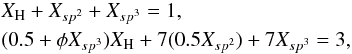 (45)which, upon re-arrangement, gives
  (46)where a = 0.5, b = 3.5 and c = (7 + φXH). Substituting into Eqs. (20)–(22) we have
 ![Mathematical equation: \begin{eqnarray} &&R = \frac{(6X_{\rm H}-1)}{(8-13X_{\rm H})+2 \phi X_{\rm H}(1-X_{\rm H})}, \\ &&\bar{m} = \frac{(20-8X_{\rm H})+2 \phi X_{\rm H}(3-2X_{\rm H})}{(7+2 \phi X_{\rm H})}, \\ &&\bar{m_{\rm C}} = \frac{(20-15X_{\rm H})+6 \phi X_{\rm H}(1-X_{\rm H})}{[7+2 \phi X_{\rm H}(1-X_{\rm H})]}, \end{eqnarray}](/articles/aa/full_html/2012/04/aa17623-11/aa17623-11-eq107.png)
 |
Fig. 2 R as a function of XH for the best-fit RCN model (Eq. (52), lower solid red line) and DG model (with L = 2, Eq. (75), lower dashed red line); the corresponding values of mC for each model are shown in the upper “flatter” red lines. Shaded: validity-ranges for the RCN (right) and DG (left) models, darker where they overlap. Thick dash-dotted: mean number of rings per aromatic cluster (NR/10). Thin dash-dotted: mean number of C atoms per aromatic cluster (nC/20). Short dashed: aromatic domain size (da in nm). Long-dashed: aromatic coherence length (La in nm). Diamonds; laboratory data for R (Angus & Jansen 1988, and references therein). |
If we now include the aromatic clusters back into this model with the methyl groups included then the eRCN equations (Eqs. (10) and (11)) can now be re-written in the form ![Mathematical equation: \begin{eqnarray} &&X_{\rm H} + X_{sp^2} + X_{sp^3} = 1, \\ &&0.5 X_{\rm H} + \{7 [0.5(1-f)]+Zf \} X_{sp^2} + (7+\phi X_{\rm H}) X_{sp^3} = 3, \end{eqnarray}](/articles/aa/full_html/2012/04/aa17623-11/aa17623-11-eq114.png) \arraycolsep1.75ptwhere a = 0.5, b = { 7 [0.5(1 − f)] + Zf } = 0.5(7 − Yf) and c = (7 + φXH). Using Eqs. (20)–(22) and substituting for a,b and c using
\arraycolsep1.75ptwhere a = 0.5, b = { 7 [0.5(1 − f)] + Zf } = 0.5(7 − Yf) and c = (7 + φXH). Using Eqs. (20)–(22) and substituting for a,b and c using ![Mathematical equation: \begin{eqnarray*} (c-b) &=& 0.5[(7+2 \phi X_{\rm H})+Y_f] , \\ (c-3) &=& 0.5(8+2 \phi X_{\rm H}) , \\ (c-a) &=& 0.5(13+2 \phi X_{\rm H}) , \\ (b-a) &=& 0.5(6-Y_f)~{\rm and} \\ (b-3) &=& 0.5(1-Y_f) , \end{eqnarray*}](/articles/aa/full_html/2012/04/aa17623-11/aa17623-11-eq117.png) we obtain R, and the average coordination numbers, and , for our most sophisticated eRCN network, i.e.,
we obtain R, and the average coordination numbers, and , for our most sophisticated eRCN network, i.e., 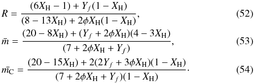 The above expression for R is plotted in Figs. 1 and 2, where we see that Eq. (52) gives a better fit to the laboratory data for the hydrogen-rich amorphous carbons. Here we have empirically assumed φ = 30(XH − 0.5)2, in order to give a physically-reasonable fit to the steep rise of R at high XH, and note that the fit is not particularly sensitive to the detailed form of the expression for φ.
In Fig. 2 we also plot other key quantities, namely: the number of rings per aromatic domain, NR = [5.8/4.3XH] 2, the aromatic domain size, da = 0.18(3NR + 4)0.5 nm, and the aromatic coherence length, La = 0.77/Eg(eV) nm ≡ 0.77/(4.3XH) nm (see Appendix A for more details).
Designation of, and formulæ for, the major eRCN bulk material structural groups.
2.2.3. A compositional de-construction of eRCNs
In this section we quantitatively examine the chemical compositional make-up and bonding configurations of eRCN-modelled a-C:Hs, i.e., we determine their C-Hn and (C-C)m bond fractions. This is done with the ultimate view of being able to predict the XH- and size-dependent, infrared spectral characteristics of these materials using the laboratory-measured cross-sections and intensities for the constituent structures (e.g., Ristein et al. 1998). The derived structures have a key bearing on the electronic and optical properties of these materials.
In “de-constructing” the network in this way we need to consider all of the possible, fundamental and basic CnHm (n ≥ 1, m ≥ 0) building blocks that make up solid, amorphous hydrocarbons. Table 1 presents the major bond groupings that we will consider in this study, gives their eRCN designations and the expressions that define their atomic fractions (derived later within this section).
The eRCN model clearly cannot account for the presence of interstitial H atoms because they do not affect the network, nevertheless their effects could be important (e.g., Sugai et al. 1989; Duley 1996; Duley & Williams 2011) and will need to be taken into account in more sophisticated models.
Note that, as above, we assume that any sp1 C-H or C ≡ C bonds are of such low abundance that their presence within, and influence upon, the eRCN model of the a-C:H structure and composition can be ignored without loss of generality (e.g., Robertson 1986; Kassavetis et al. 2007). Similarly, we also ignore the possible incorporation of oxygen and nitrogen atoms into the hydrocarbon structure. Although, the addition of sp1 carbon atoms and hetero-atoms could, in principle, be incorporated into a further extension of the eRCN formalism, with the inclusion of structure-terminating and bridging groups such as – C ≡ C –, ≡ C–H, – O – , – OH, = O, – NH2, = NH and the substitution of N for C in aromatic rings. However, and in practice, it is difficult to do this in a physically-meaningful way because of the inherent limitations of the method (see Appendix B). Dadswell & Duley (1997) have in fact already considered the incorporation of O atoms, in the form of OH groups, into the RCN structure and find that this can lead to a strong absorption feature in the 3 μm region.
In their work on a-C, a-C:H and ta-C materials, with band gaps in the range 0 − 3 eV, Kassavetis et al. (2007) find that their two Tauc-Lorentz (2-TL) oscillator model, for the optical properties, does not give an entirely satisfactory fit for a-C:H materials. They suggest that this is due to the presence of sp1 bonds and chain-like configurations that are inconsistent with the assumptions of their model. There is now convincing analytical and experimental evidence to support this suggestion because as-deposited, hydrogen-free, cluster-assembled carbon films can exhibit a significant sp1 carbon chain component, which is almost completely destroyed upon exposure to air (e.g., Ferrari & Robertson 2004).
As pointed out by Ferrari & Robertson (2004), the nature of the clustering of the sp2 phase (into chains or cage-like structures) and the orientation of those clusters can play a key role in the determination of the properties of amorphous (hydro)carbon materials.
Using femtosecond pulsed laser ablation and deposition to form tetrahedral carbon and amorphous diamond-like films Hu et al. (2007a,b) find that the composition of these materials includes sp1, sp2, and sp3-bonded carbon. They show that an observed excitation band in their UV-Raman spectra (2000 − 2200 cm-1 ≡ 4.55 − 5.00 μm) is consistent with the presence of sp1 chains in their materials, with sp1 carbon atom fractions of ≈ 6%. This work clearly provides a key insight into the detailed composition and structure of tetrahedral carbon films containing sp2 clusters and sp1 chains. However, it yet remains to be seen whether the properties of these (hydrogen-poor) materials, often produced under “stressful” conditions, can be applied to interstellar carbonaceous particles formed under less-intense energy conditions and where exposure to H atoms is practically ubiquitous.
Interest in the inclusion of nitrogen into amorphous carbons has led to the study of amorphous carbon nitrides, a-CNx, in which various N-bonding configurations have been classified (e.g., Ferrari & Robertson 2004). In their detailed study, Dartois et al. (2005) found that if nitrogen atoms are present in laboratory analogues of interstellar amorphous hydrocarbons then they tend to be found in structure-bridging groups rather than being incorporated into aromatic clusters. However, the similar frequencies for C–C and C–N modes does make the interpretation of the skeletal modes rather difficult (e.g., Ferrari & Robertson 2004). In general, a low content or absence of “hetero-atom” groups in ISM carbonaceous materials is apparent (Pendleton & Allamandola 2002; Dartois et al. 2005) and hence the simplifying assumption to ignore them here is justified. Nevertheless, there are indications for a carbonyl component (characteristic of ketones) in the carbonaceous dust in the Seyert galaxy NGC 1068 (Dartois et al. 2004a). Additionally, the incorporation of O and N into the CHON-type materials (in CHON, CH, CHO and CHN combinations) detected in the comet Halley dust (e.g., Clark et al. 1987) implies that the incorporation of O and N hetero-atoms into the eRCN structure could be important for solar system studies. However, such an extension of the eRCN model is not without its limitations, as pointed out in Appendix B.
We note that the expressions for the C-C bonds in Table 1 follow trivially from the earlier-defined expressions for the sp2 and sp3 carbon atom content of the eRCN (e.g., see Sect. 2.1). For the more abundant C-H bond configurations we adopt a simple statistical approach to arrive at the C-H bond definitions, i.e., we assume an equipartition of the hydrogen atoms between the sp2 and sp3 carbon atom sites where the H atoms can bond. Based on this assumption we derive expressions for the aromatic CH, olefinic CHn (n = 1,2) and aliphatic CHn (n = 1,2,3) bond concentrations.
For (e)RCNs the case where XH = 0.5 provides something of a critical point, which corresponds to structures with (H/C) = 1, i.e., where, statistically, each carbon atom is associated with one hydrogen atom. We therefore now consider the two regimes, XH ≤ 0.5 and XH > 0.5, in our de-construction of the eRCN bonding. In both cases the hydrogen-to-carbon atom concentration ratio can be expressed as, ![Mathematical equation: \begin{equation} \frac{[H]}{[C]} = \frac{X_{\rm H}}{(1-f)X_{sp^2}+X_{sp^3}} = \frac{X_{\rm H}}{(1-X_{\rm H})-fX_{sp^2}} \equiv \eta, \end{equation}](/articles/aa/full_html/2012/04/aa17623-11/aa17623-11-eq176.png) (55)where the denominator is the olefinic sp2 and aliphatic sp3 carbon atom fraction. As can be seen, we have for the moment, ignored the aromatic carbon and its associated hydrogen content, as indicated by the − fXsp2 term in the denominator. We return to this missing aromatic carbon component later in this section.
(55)where the denominator is the olefinic sp2 and aliphatic sp3 carbon atom fraction. As can be seen, we have for the moment, ignored the aromatic carbon and its associated hydrogen content, as indicated by the − fXsp2 term in the denominator. We return to this missing aromatic carbon component later in this section.
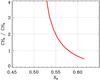 |
Fig. 3 The CH2/CH3 abundance ratio as a function of XH for the aliphatic carbon component in the best-fit eRCN model (Eq. (52)). |
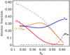 |
Fig. 4 The aromatic, fXsp2 (red), olefinic, (1 − f)Xsp2 (orange), total sp2, Xsp2 (grey dashed), aliphatic, Xsp3 (blue) and CH3, φXsp3 (black dashed), carbon atom fractions as a function of XH for the best-fit eRCN model (Eq. (52)). |
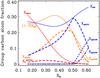 |
Fig. 5 As for Fig. 4 with the aromatic ( |


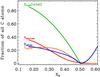 |
Fig. 6 The fraction of all carbon atoms (XC,noH(total), green), sp2 aromatic (Xsp2,ar,noH, red), olefinic (Xsp2,noH, orange) and sp3 (Xsp3,noH, blue) carbon atoms as a function of XH that are not attached to a hydrogen atom, for the best-fit eRCN model (Eq. (52)). |
Figure 3 shows the CH2/CH3 abundance ratio as a function of XH for the aliphatic carbon component in the best-fit eRCN model. In the diffuse ISM this ratio appears to be 2.5 ± 0.4 (Pendleton & Allamandola 2002) and in laboratory a-C:H is close to 2 (Dartois et al. 2005), which would seem to imply, based on the eRCN model, that the large carbonaceous grains in the ISM, that are observed in absorption, must be rather H-rich with XH lying in a narrow range close to ~0.53−0.55 and a H/C ratio of the order of 1.2.
For XH ≤ 0.5 each carbon atom is, at most, singly hydrogenated (see above) and we can ignore CH2 and CH3 groups. We then have  (56)
where i = 2 (i = 3) corresponds to single sp2 olefinic CH (sp3 aliphatic CH) bonds, and u is an aromatic C-H abundance re-normalising factor (see Table 1). Xi represents the corresponding carbon atom fraction, i.e., (1 − f)Xsp2 or Xsp3. Particularly important in the case of these hydrogen-poor eRCNs is the need to consider the sp2 (polycyclic) aromatic cluster hydrogen content. From Table A.1 (see also Fig. A.2) we can see that the aromatic cluster coordination number per carbon atom for an aromatic cluster is given by the cluster coordination number, mcluster, divided by the number of constituent carbon atoms, nC,
(56)
where i = 2 (i = 3) corresponds to single sp2 olefinic CH (sp3 aliphatic CH) bonds, and u is an aromatic C-H abundance re-normalising factor (see Table 1). Xi represents the corresponding carbon atom fraction, i.e., (1 − f)Xsp2 or Xsp3. Particularly important in the case of these hydrogen-poor eRCNs is the need to consider the sp2 (polycyclic) aromatic cluster hydrogen content. From Table A.1 (see also Fig. A.2) we can see that the aromatic cluster coordination number per carbon atom for an aromatic cluster is given by the cluster coordination number, mcluster, divided by the number of constituent carbon atoms, nC,  (57)where we have here assumed that the aromatic clusters are compact. Figure A.2 shows the behaviour of mar as a function of the number of aromatic rings, NR, in the cluster. Appendix A gives the details of the aromatic cluster characterising parameters. For the aromatic C-H fraction we then have
  (58)For XH > 0.5, a carbon atom can be multiply hydrogenated and we therefore need to calculate the concentrations of CHn groups for sp2 (where i = 2 and n = 1 or 2) and sp3 (where i = 3 and n = 1, 2 or 3). In this case it can be shown that, for n = 1 and 2,
 ![Mathematical equation: \begin{equation} X^i_{{\rm CH}_n} = u \, n \, [(-1)^n (n \eta-2)] \, X_i \, \left[ \ +0_{\ (i=2)}, \ -\frac{1}{3} X^3_{{\rm CH}_3, \ (i=3)} \ \right], \end{equation}](/articles/aa/full_html/2012/04/aa17623-11/aa17623-11-eq205.png) (59)where the term in the left hand square brackets gives (2 − η), for CH groups, or 2(η − 1), for CH2 groups (see Table 1), and is a C-H bond abundance factor. For the fractional abundance of methly groups, i.e., n = 3 (see Sect. 2.2.2), we have
(59)where the term in the left hand square brackets gives (2 − η), for CH groups, or 2(η − 1), for CH2 groups (see Table 1), and is a C-H bond abundance factor. For the fractional abundance of methly groups, i.e., n = 3 (see Sect. 2.2.2), we have  (60)Figures 4 and 5 show the carbon atom and CHn bond fractions, derived using the expressions (indicated in full in Table 1), as a function of XH for the best-fit eRCN model (Eq. (52)). The general trends to be seen in these figures are that, with decreasing XH, H-rich aliphatics give way to H-poorer olefinics and aromatics, and that sp3 CH3 and CH2 groups are progressively replaced by CH2 and then CH olefinics. Note that the aromatic CH abundance is rather low in these materials, which even in their H-poorest state contain more, and about equal fractions of, aliphatic and olefinic CH groups.
In Fig. 6 we show the fractions of the eRCN constituent carbon atoms that are not bonded to a hydrogen atom. The indicated trends are rather similar with the, not-unexpected, exception that for low values of XH most of the aromatic sp2 carbon atoms are not hydrogenated, as can clearly be seen by comparison with Fig. 5.
2.2.4. The predicted infrared spectra of bulk eRCN materials
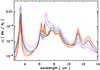 |
Fig. 7 The adopted wavelength-dependent, IR band cross-sections per carbon atom, σC (1 Mb = 10-18 cm2), for the eRCN model as a function of XH ( ≡ Eg). The upper curves (purple) are for the H-rich, wide band gap materials and the cross-sections, in the 8 μm region, decrease with decreasing XH from top to bottom – XH = 0.58 (purple), 0.52 (cobalt), 0.46 (blue), 0.40 (green), 0.34 (yellow), 0.29 (orange), 0.23 (brown) and 0.17 (red). |
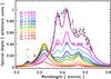 |
Fig. 8 The predicted eRCN spectrum in the 3.2−3.6 μm C-H stretching region as a function of XH calculated using the structural de-composition described in Sect. 2.2.3 and the data in Table 2. The diamonds, squares and triangles indicate the aliphatic, olefinic and aromatic band positions, respectively (see Table 2). The data with error bars are for the diffuse ISM absorption along the Galactic Centre IRS6E line of sight (black) and Cyg OB2 No. 12 (grey) (taken from Pendleton & Allamandola 2002). |
Adopting a compositional structure and the appropriate band parameters allows a prediction of the IR spectra, as was done for HAC materials in the 3 μm region (e.g., Duley 1995; Dadswell & Duley 1997; Duley et al. 2005a). This kind of study then enables a search for RCN solutions that would be compatible with observations (e.g., Duley 1995).
Using typical C-H and C-C band positions, widths and cross-sections taken from the literature (see Table 2 and references therein, and Fig. 7) and the eRCN structural de-construction described in Sect. 2.2.3 and Table 1, we show the predicted optical depth spectra τ(ν), in arbitrary units, for bulk eRCN materials in the 3 μm and 6−7 μm regions in Figs. 8 and 9, respectively. Here the optical depth normalised by the C atom column density, NC, is given by 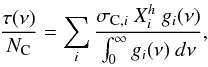 (61)where σC,i is the integrated cross-section per C atom for band i (see Table 2 and Fig. 7),
  is the relative abundance (atomic fraction) for group i (CnHm, where n = 1,2 and m = 0,1,2,3) of C atom hybridisation state h (where 2 ≡ sp2 or 3 ≡ sp3, in keeping with the nomenclature used in Tables 1 and 2) and g(ν) is the band profile. Anticipating the required behaviour of these bands at long wavelengths (FIR to cm), we here assume intensity-normalised, Drude profiles for all of the bands, i.e.,
  (62)where ν is in wavenumbers, ν0 is the band centre and γ the band width. The spectra in Figs. 8 and 9 have been normalised to the peak of the strongest band exhibited for all of the displayed, XH-dependent compositional spectra (i.e., the 3.42 band in the XH = 0.615 sample). In Fig. 10 we show the same spectral data but normalised to the strongest band in each spectrum in order to better indicate the evolution of the form of the spectra as a function of XH.
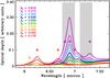 |
Fig. 9 The predicted eRCN spectrum in the 6.0−7.5 μm C-H bending and C-C mode region as a function of XH calculated using the structural de-composition described in Sect. 2.2.3 and the data in Table 2. The symbols are the same as for the previous figure. The grey shaded areas indicate the approximate full width of the observed a-C:H bands in this region (e.g., Pendleton & Allamandola 2002; Dartois et al. 2005). |
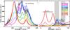 |
Fig. 10 The predicted full eRCN spectrum in the 3−8 μm C-H stretching and bending and C-C mode region as a function of XH calculated using the structural de-composition described in Sect. 2.2.3 and the data in Table 2. Here the spectra are normalised to the strongest band for each value of XH. The data with error bars and the shaded areas indicate the diffuse ISM bands as per Figs. 8 and 9. |
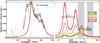 |
Fig. 11 The predicted full DG spectrum in the 3−8 μm C-H stretching and bending and C-C mode region as a function of XH calculated using the structural de-composition described in Sect. 2.2.3 and the data in Table 2. Here the spectra are normalised to the strongest band for each value of XH. On the left the strongest bands are for high XH > 0 (green to brown), while the opposite is true for the longer wavelength bands on the right (shortward of 6.8 μm). The data with error bars and the shaded areas indicate the diffuse ISM bands as per Figs. 8 and 9. |
Adopted C-H and C-C band modes in eRCN bulk materials: band centre (ν0), width (δ) and integrated cross-section (σ).
From Figs. 8–10 it can clearly be seen that, as XH decreases, the band intensities weaken with the transition from aliphatic-dominated structures to olefinic and aromatic-rich materials. It is interesting to note, from a close look at Figs. 8 and 9, that there is a rather clear separation of the spectral properties of eRCNs at XH ~ 0.5 as the dominant structure changes from aliphatic to olefinic/aromatic. Indeed the structure and spectra of eRCNs evolve “rapidly” in the region 0.5 < XH < 0.62 (cf. the steepness of R in this region of XH in Fig. 1), as a result of the loss of aliphatic material, and then evolve more “slowly” for XH < 0.5, where the transition is principally from olefinic to aromatic composition as the sp2 regions “coalesce” into larger aromatic domains as XH decreases. Thus, and as expected from the cross-sections indicated in Table 2, at low XH the spectra show only the relatively weaker aromatic bands occurring at shorter wavelengths than for the aliphatic, H-rich eRCNs (XH > 0.5) in both of the spectral windows shown in Figs. 8–10.
2.3. The defective graphite (DG) model for H-poor amorphous hydrocarbons
As shown above the eRCN model is only valid for amorphous hydrocarbons with XH ≳ 0.2. For H-poor amorphous hydrocarbons we therefore need to develope a new approach to modelling their structural properties. In order to do this we adopt and modify the “defective graphite” (DG) formalism of Tamor & Wu (1990), which considers carbon atom vacancies in an otherwise perfect graphite lattice. Such vacancies leave the three adjacent carbon atoms, which are supposed to transform from sp2 to sp3, each with two dangling bonds because the contiguity of the aromatic structure has been broken. Essentially, this lattice vacancy approach is a percolation issue because, with increasing vacancy concentration, a percolation threshold is reached, which is the point where the aromatic domains cease to percolate and become isolated (e.g., Stauffer & Aharony 1994). Ultimately all aromatic character will be lost at some higher vacancy concentration.
Figure 12 shows a graphite basal plane with two carbon atom vacancies, and indicates the essential elements of the DG network model. In Fig. 12 the lower, left defect contains three radical carbon atoms and results in a loss of the aromatic character in the three concerned rings. Each carbon atom adjacent to a defect (carbon atom vacancy) can then be “passivated” by the addition of two hydrogen atoms, to form three associated sp3 CH2 groups within the graphite basal plane. The loss of one carbon atom is then compensated by the addition of six hydrogen atoms. In the upper right defect the three adjacent carbon atoms have been transformed to sp3 and each has been bonded to two hydrogen atoms. In this case there is an associated loss of the aromatic character in six adjacent rings.
 |
Fig. 12 The defected graphite (DG) network model. The filled (open) circles represent carbon (hydrogen) atoms in an aromatic network. The inset dotted circles indicate rings with aromatic character. |
If we now consider a defect-free, graphite lattice with NC carbon atoms, into which we introduce Nv carbon atom vacancies (defects) each of which is associated with six hydrogen atoms, then 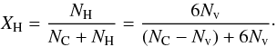 (63)If we now define the vacancy fraction within the defective graphite lattice as Q = (Nv/NC) then
 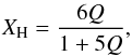 (64)where the total number of carbon and hydrogen atoms in the lattice is (1 + 5Q). The number of sp3 sites is then 3Nv and their atomic fraction is 3(Nv/NC) ≡ 3Q. Similarly, the atomic fraction
of sp2 sites is 1 − (Nv/NC) − 3Q = 1 − 4Q and for the DG model we can write  Substituting for Q using Eq. (64), i.e., Q = XH/(6 − 5XH), we then have
 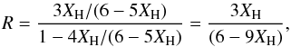 (68)which indicates that the range of validity for the DG model is 0 ≤ XH ≤ 0.66. However, the upper limit here is really determined by the defect concentration and the defected graphite metal-to-insulator transition. Tamor & Wu (1990) determine that this key transition occurs at Q = 1/24 ( ≡ 0.042) or, equivalently (via substitution into Eq. (64)), for XH = 0.21. We note that for Q > 1/12 (XH > 0.35) the structure is no longer a contiguous network and so XH = 0.35 (i.e., a composition of ≈ CH0.3 or C3H) represents a “hard” upper limit to XH and the validity of the DG model.
From the point of view of percolation, a hexagonal (honeycomb) lattice has a percolation threshold pc = 0.6962, which is the minimum site concentration for an infinite network in an infinite lattice (e.g., Stauffer & Aharony 1994). The critical vacancy threshold is then (1 − pc) = 0.3038. However, in this infinite honeycomb network not all sites are part of hexagonal ring systems and so this is not an appropriate model for a contiguous aromatic lattice, where each 6-fold aromatic ring is made up of six carbon atoms each shared by three rings ( , i.e., two carbon atoms per ring). Given that, and that each vacancy leads to the de-aromatisation of three rings (with no H atom addition), the critical vacancy threshold for a contiguous aromatic network is then (1 − pc)/(2 × 3) = 0.051, which is very close to the critical defect concentration of 0.042 for the metal-to-insulator transition in graphite found by Tamor & Wu (1990). Thus, for vacancy concentrations larger than ≃ 0.04 the percolation threshold is reached and the aromatic domains no longer percolate but become isolated from one another.
A lower limit to the H atom content of amorphous hydrocarbons comes from the results of irradiation studies, which show that H atom loss from a-C:H stops at about XH ≈ 0.05 (e.g., Adel et al. 1989; Marée et al. 1966; Godard et al. 2011). Such a lower limit to the DG model validity, and as an indicator of the minimum possible H atom content in processed a-C:H materials, could have important consequences for the evolution of dust under ISM conditions if this same lower limit holds true there. For a further discussion on this point see Paper II (Sect. 5.2).
In the same way as for the eRCN model we can derive the average atomic coordination number, m, and average carbon atom coordination number, mC, which are 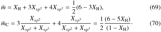 The fraction of sp2 atoms in aromatic rings is equal to Xsp2 in the DG case because all of them are part of a ring, therefore substituting for Q = XH/(6 − 5XH) from Eq. (64) we get the fraction f of the carbon atoms in aromatic rings
 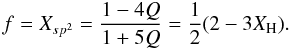 (71)Note that the above formalism implicitly takes into account the de-aromatisation of that part of the graphite lattice associated with the defect (i.e., the conversion of carbon atoms from sp2 to sp3), and therefore Xsp2 is a direct measure of the aromatic carbon atom fraction.
If we now consider the DG model in terms of stacked graphite sheets then we can see that defects (vacancies) in close proximity in adjacent sheets could lead to cross-linking between the layers. We note that nitrogen hetero-atoms could perhaps play an important role here because in nano-structured a-C:N films a strong cross-linking between graphitic planes is observed (e.g., Ferrari & Robertson 2004). In any event, cross-linking leads to a reduction in the hydrogen atom content for a given value of R by at least one hydrogen atom per defect. The loss of more than one hydrogen atom per defect, up to a maximum of three per defect, implies multiple cross-links per defect. A minimum condition for all of the stacked DG layers to cross-link into a macroscopic structure is when each vacancy is associated with two cross-links, each forming an aliphatic bridge to one of the two adjacent sheets. We further assume that the cross-links on the sp3 carbon atoms can, for steric hindrance reasons, only be on adjacent sp3 carbon atoms. Thus, both CH2 and CH groups can be present in the DG structure. If L is the number of cross-links per defect (0 ≤ L ≤ 3) then the number of hydrogen atoms per defect is (6 − L)Q and we have that 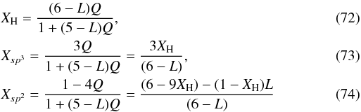 and
and  (75)where we use the substituion
  (76)We can also re-formulate Eqs. (69) and (70) for the atomic coordinations for cross-linked DG structures using this substitution for Q i.e.,
 ![Mathematical equation: \begin{eqnarray} &&{\bar m} = \frac{(6-3X_{\rm H})-(1-X_{\rm H})L}{2 -\frac{1}{3}(1-X_{\rm H})L}, \\ &&{\bar m_{\rm C}} = \frac{3[(6- 5X_{\rm H})-(1-X_{\rm H})L ]}{(6-L)(1-X_{\rm H})}, \end{eqnarray}](/articles/aa/full_html/2012/04/aa17623-11/aa17623-11-eq289.png) which reduce to Eqs. (69) and (70) when L = 0.
which reduce to Eqs. (69) and (70) when L = 0.
Figure 2 shows the results for the DG model of Eq. (75), over its range of validity 0 ≤ XH ≤ 0.35, assuming L = 2, i.e., that there are two cross-linking bonds per defect (carbon atom vacancy). As can be seen in Fig. 2, this DG model gives reasonable agreement with the eRCN model and has the advantage that it can be used to describe hydrogen-poorer hydrocarbons extending towards a graphite-like structure. Also shown in Fig. 2 are the mean carbon atom coordination numbers,  , for the eRCN (solid red line) and DG (dashed red line) models.
2.3.1. A compositional deconstruction of bulk DGs and their predicted infrared spectra
In the same way as was done for eRCNs (see Sect. 2.2.3) we can deconstruct the DG network into its component structures. However, in this case the process is much simplified because the network consists of only aromatic sp2 carbon atoms and aliphatic CH and CH2 groups (at the vacancy sites). We then have, respectively, for the aromatic and aliphatic C-C bonds and the aliphatic CH and CH2 groups concentrations:  , XC − C,DG = 2Xsp3, XCH2,DG = (3 − L) Xsp3 and XCH,DG = L Xsp3. Note that these equations indicate that the number of inter-atomic bonds is not equal to the total number of atoms in the structure. Thus, the atomic bond fractions have to be normalised by the total number of bonds, Xbond, which is given by
 ![Mathematical equation: \begin{eqnarray} &&X_{\rm bond} = \frac{3}{2} X_{sp^2}\ +\ 2\, X_{sp^3}\ +\ X_{\rm H} \notag\\ &&\ \ \ \ \ \ \ \ \ \, = \frac{3}{2} X_{sp^2}\ +\ \left[2+\frac{(6-L)}{3} \right] X_{sp^3} \label{eq_DG_bond_renorm} \end{eqnarray}](/articles/aa/full_html/2012/04/aa17623-11/aa17623-11-eq297.png) (79)where we have substituted
(79)where we have substituted  . We then have for the DG model that the atomic bond fractions in the structure are
  The only spectral bands that bulk DGs will show are therefore at 6.25 and 6.67 μm due to aromatic C ≃ C bonds, 3.45 μm due to aliphatic CH stretching, 3.42 and 3.51 μm due to aliphatic CH2 stretching modes, and at 6.9 μm due to aliphatic CH2 bending (e.g., see Table 2). However, for finite-sized particles the surface bonds will be terminated with H atoms and a large fraction of these will be aromatic CH bonds; as at the periphery of isolated polycyclic aromatic hydrocarbon (PAH) molecules. These DG particle, aromatic, surface CH bonds could provide a catalytic rôle in molecular hydrogen formation in the ISM (e.g., Rauls & Hornekær 2008; Le Page et al. 2009) and such processes, involving CH2 sites, could lead to a significant fraction of surface (or PAH “edge”) aliphatic CH2 groups, in addition to the aromatic CH sites. The consequences of particle size for the DG model are discussed in detail in a following paper.
3. The 3–13.5 μm spectra of hydrocarbon solids
In Fig. 13 we show the full, but provisional, spectra presented as the absorption coefficient, α, for our eRCN/DG materials. These spectra are well-constrained for wavelengths less than ≃7.3 μm where the band cross-sections have been determined experimentally. However, for the longer wavelength bands, and as indicated in the lower part of Table 2 (i.e., bands 20 to 27), we have introduced “place holder” bands with positions, widths and intensities, determined by comparison with a-C:H absorption coefficient data (taken from Robertson 1986, Fig. 14), and also guided by the band positions and widths in the interstellar emission spectra (e.g., Verstraete et al. 2001), with the aim of allowing a qualitative exploration of the behaviour of the spectral variations of these materials in the ISM. However, some progress in this area has been made with the measurement of the absorption and emission spectra of some HAC materials and carbon nano-particles in the 3 to 20 μm wavelength region (e.g., Scott et al. 1997; Duley et al. 2005a,b; Hu et al. 2006; Hu & Duley 2008a,b).
We caution the reader in the use of the spectral bands longward of 7.3 μm for the detailed interpretation of astronomical spectra, at least until such time as these bands have been measured in the laboratory for a wide range of amorphous hydrocarbon solids. Nevertheless, the adaptability of this model will allow for a rather easy revision of the complex index of refraction data once appropriate laboratory data become available.
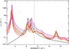 |
Fig. 13 The predicted eRCN and DG spectra, presented as the absorption coefficient, α, in the 2.5 − 13.5 μm region as a function of Eg calculated using the structural de-composition described in Sects. 2.2.3, 2.2.4 and 2.3 and for the data in Table 2. The adopted colour-coding for this plot is from large band gap (2.67 eV, purple) to low band gap (–0.1 eV, black) with intermediate values in steps of 0.25 eV from 2.5 (violet) to 0 eV (grey) with the addition of the Eg = 0.1 and − 0.1 eV cases (light grey and black, respectively), as per Paper II. The bands with central positions long-ward of the vertical grey line (λ(ν0) > 7.3 μm) are not yet well-determined by laboratory measurements. |
We note that the spectra shown in Fig. 13 exhibit most of the IR bands observed in absorption and in emission in the ISM and that the model predicts a general weakening of the aliphatic bands, as XH decreases, which is accompanied by a shift in character towards olefinic and aromatic-dominated bands. We also note that the relative intensities of the bands will depend upon particle size and not just on XH. This effect will be studied in detail in a follow-up paper.
4. Astrophysical implications
The evolution of the spectral properties of carbonaceous dust, from its formation in the circumstellar shells around evolved stars to its transition into the ISM, has clearly been demonstrated (e.g., Goto et al. 2003, 2007; Sloan et al. 2007; Pino et al. 2008). The eRCN/DG carbonaceous dust evolution model presented here, in which the nature of the dust is characterised by its hydrogen content, XH, and the carbon atom sp3/sp2 hybridisation ratio, R = Xsp3/Xsp2, allows a detailed exploration of the compositional transformations of these types of materials.
We now examine some of the consequences of hydrogenated amorphous carbon dust evolution, as predicted by the eRCN and DG models, within the astrophysical context. However, a full examination will be presented in a follow-up paper, once the optical properties (Paper II) and the size dependence of these properties have been investigated.
4.1. Structural variations and spectral properties
As a result of the effects of photo-darkening, aromatisation or “graphitisation” of a-C:H solids there is a transformation of carbon atoms from the sp3 to the sp2 hybridisation state that is necessarily accompanied by a net loss of H atoms from the structure (e.g., Duley 1996). The eRCN/DG model predicts a maximum hydrogen content of about 62%, which is in good agreement with experiment. Conversely, after extreme processing, it appears that practically all of the hydrogen can be removed from these materials. Ion irradiation experiments indicate a minimum H atom content of about 5% but amorphous carbon materials formed in the laboratory can be made essentially hydrogen free and so it is expected that the lower limit is therefore “H-free” materials.
In the ISM the large carbonaceous grains appear to have a CH2/CH3 ratio in the range ~ 2 − 3 (e.g., Pendleton & Allamandola 2002; Dartois et al. 2005). Fig. 3 indicates that, for the eRCN model, this would be equivalent to a rather narrow hydrogen atom fraction range, i.e., ~ 53 − 55% ( ≡ XH = 0.53 − 0.55). However, looking at Figs. 8, 9 and 10 we can see that it is the predicted spectra for a-C:H materials with XH ≥ 0.57 that appear to be more consistent with the absorption observed along the Galactic Centre IRS6E, Cyg OB2 No. 12 and IRS7 lines of site (e.g., Pendleton & Allamandola 2002; Dartois et al. 2004b) and towards Seyfert 2 galaxy nuclei by Dartois et al. (2004a) who identify the source material as being of a-C:H origin. We note that XH ≥ 0.57 implies a CH2/CH3 ratio ≃ 1 (see Fig. 3), rather than the expected value of ~ 2 − 3. Thus, while the spectal agreement is rather good in the 3 − 4 μm region, it does not appear to be coherent with the observed CH2/CH3 ratio. As indicated in Table 2, we needed to increase the intensity of only the 3.38 μm CH3 band in order to obtain a good match to the observational data. Thus, the discrepancies noted here could be due to uncertainties in the band strengths and/or assignments and/or to particle size effects.
The intrinsic CH, CH2 and CH3 groups responsible for the suite of absorption features around 3.4 μm show a clear transformation from sp3-dominated CHn bands to sp2-dominated CHn bands as aromatisation proceeds and as XH declines (see Figs. 4 and 5). The accompanying spectral variations shown in Figs. 10 and 11 predict that the spectrum evolves towards one dominated by olefinic and aliphatic CH groups, with bands at 3.32 and 3.47 μm in the case of eRCN, and only aliphatic CH and CH2 bands at 3.42, 3.45, 3.47 and 3.51 μm for the DG model. We note that the aromatic CH band at 3.28 μm is not apparent in these spectra because of the lower abundance of the aromatic CH groups (with respect to olefinic and aliphatic CH groups) in the eRCN model and also because its lower intrinsic absorption strength (see Table 2). Aromatic CH bands are expected in the DG spectra but they are not included here, i.e., the DG spectra do not yet take into account the likely hydrogenation of the aromatic surface nor the possibility of aromatic CH formation at defect sites. These aspects will be dealt with in detail in following paper.
The evolution of the structural and spectral properties of a “single” carbonaceous material therefore appears to provide a good model for the evolution of amorphous hydrocarbons in interstellar and circumstellar media. With the addition of surface hydrogenation, and additional size effects, to the calculation of the spectra the DG model can be carried forward to a study of the most aromatic carbon particles in the ISM. These will necessarily be the smallest particles, UV-photo-darkened and stochastically-heated to high temperatures, as a result of which they will be dehydrogenated and aromatised.
The sp3 to sp2 transition, as a result of UV photo-processing in the ISM, could possibly be counterbalanced by hydrogen atom addition to the structure as a result of (energetic) collisions (e.g., Duley 1996). However, it is not yet clear that this “reverse” process of ‘aliphatisation’ can occur because it requires that the incident H atoms are energetic enough to insert into aromatic rings and transform sp2 C atoms into sp3 sites. Given that the aromatic C ≃ C bond energy in benzene is of the order of 5 eV, and that for an H atom to insert it must break at least one CC bond, the activation energy for this process is at least 5 eV, equivalent to >5 × 10⁴ K, which would seem to indicate that there is a significant energy barrier to a-C/a-C:H hydrogenation in the ambient ISM. However, this is offset by the formation of an aromatic CH bond (~4.3 eV) and thus, if quantum mechanical tunnelling can occur, the barrier to aliphatisation could be as low as 0.7 eV ( ≈ 8000 K). These types of interactions have been well-studied experimentally and theoretically by Duley (2000) and Mennella (2008, 2010), within the context of carbonaceous dust evolution in dense regions, and we therefore do not enter into any further speculation on the aliphatisation issue here.
4.2. H2 formation in PDRs via a-C:H de-hydrogenation?
Recent observations and their interpretation appear to require rather efficient molecular hydrogen formation at “elevated” temperatures in photon-dominated regions (PDRs, e.g., Habart et al. 2004, 2011). Rauls & Hornekær (2008) and Le Page et al. (2009) propose that H2 formation can be catalysed by reactions involving the chemical trapping of H atoms at the periphery of PAH molecules in the ISM. In a rather similar vein, we note that in a-C:H materials “UV-photolysis” or ion irradiation, resulting in an aromatisation, induces H atom loss from the structure and is associated with the in situ formation of molecular hydrogen, as studied and modelled by Smith (1984), Adel et al. (1989), Marée et al. (1966) and Godard et al. (2011).
Initially, at least, the formation of H2 and CH bonds occurs as interstitial H atoms, with binding energies of the order of 0.05 − 0.2 eV ( ≡ 600 − 2400 K), become mobile, react and are lost from the solid, consistent with an observed increase in the aliphatic 3.4 μm band intensity for temperatures above 573 K, a process that rapidly terminates at higher temperatures (e.g., Smith 1984; Sugai et al. 1989; Duley 1996).
Thus, the formation of H2 associated with the aliphatic to aromatic transformation of amorphous hydrocarbon grains should occur in PDRs where the abundant UV photons will progressively de-hydrogenate any H-rich a-C:H material that has been “ablated” or “advected” from the nearby, denser molecular regions. In this case it is the de-hydrogenation of the smallest a-C(:H) particles that could contribute most to the formation of H2 because of their relatively large abundance and the fact that they will also undergo stochastic heating to temperatures of the order of hundreds of degrees K. However, their stock of hydrogen is rather low. The reverse process of H atom addition to the aromatic component of these small carbon grains (e.g., Rauls & Hornekær 2008; Le Page et al. 2009) could offset H atom loss by UV photo-dissociation. Thus, an equilibrium between the UV and/or thermal processing of small a-C:H particles in PDRs and H atom addition could be a viable source of H2 formation at “high” dust temperatures where more classical models for H2 formation appear to be inadequate (see Paper II for a quantification of this process).
4.3. a-C:H decomposition products
It is interesting to note that the aromatisation of a-C:H materials will yield decomposition products as the materials evolve. The principal product, as discussed above, will be molecular hydrogen. However, it is likely that other species will also be released as the structure re-adjusts to a new composition. As was clearly shown by Smith (1984), a-C(:H) loses its hydrogen not just as H2 but also as hydrocarbon molecules, which leads to significant mass loss from the samples during thermal annealing. The release of “molecular” daughter species is likely to become more pronounced as the particle size decreases as suggested by Duley (1996), Scott et al. (1997), Duley (2000) and Jones (2009).
Pety et al. (2005) proposed that the small hydrocarbons, such as CCH, c-C3H2, C4H that they observed in PDRs derive from precursor PAHs. This hypothesis was proposed by Scott & Duley (1996) and extended by Jones (2009) who both postulated that the precursors for these “PAHs” themselves derive from the photo-thermal de-construction of small a-C(:H) particles (as is indeed supported by the laboratory work of Smith 1984) in the transition from dense, molecular regions of the ISM to PDRs. These precursor “PAHs” may rather resemble the locally aromatic polycyclic hydrocarbons (LAPH), cousins of PAHs, that were proposed by Petrie et al. (2003) as a carrier of the IR emission bands.
Here we follow the suggestion of Scott & Duley (1996) and Jones (2009) that a-C(:H) materials in the photon-dominated ISM follow a continuous evolutionary sequence that schematically can be represented as: a-C:H → a-C → “PAHs”/“LAPHs” → small hydrocarbons. The exact evolutionary track of the carbonaceous particles will depend upon their size. This is clearly only a part of what must be a complete carbon cycle and so the above needs to be complemented by “return journey”, i.e., a re-formation of a-C(:H) materials somewhere in the ISM, perhaps this can occur by a-C(:H) accretion onto pre-existing grains as proposed long ago by Jones et al. (1990), more recently by Jones (2009) and alluded to by Jones & Nuth (2011).
5. Predictions of the eRCN/DG model
Here we summarise some of the more important predictions of the eRCN/DG model:
-
1.
The determination of a-C:H/a-C structures, containing onlysp2 and sp3 C atoms and H atoms, and their related spectra based on only the critical H atom content, XH (or equivalently the band gap energy Eg(eV) ≃ 4.3XH), as a result of UV photon-driven and/or thermal annealing, where sp3 C atoms are transformed into sp2 C atoms as annealing proceeds.
-
2.
With annealing the a-C:H spectra “evolve” more rapidly for the hydrogen-rich materials, i.e., 0.5 < XH < 0.62, than for the hydrogen-poorer materials, due to the loss of hydrogen from the structure and the necessary major structural re-arrangement that is required to compensate for this loss.
-
3.
The expected spectrum of the large carbonaceous grains in the ISM is given by the purple spectra in Figs. 8 to 10 and 13; based on the fit to the observed interstellar absorption in the 3.2 − 3.6 μm region the spectra indicate XH ≳ 0.57 with a CH2/CH3 ratio ≈ 0.5 − 1.3 (Fig. 3).
-
4.
That the photo-thermal dehydrogenation/decomposition of a-C:H provides an efficient route to molecular hydrogen formation, and to the production of small daughter hydrocarbons (e.g., CCH, c-C3H2, C4H, etc.), in regions where their formation would otherwise appear to be inhibited.
6. Limitations of the eRCN/DG model
The eRCN and DG structural models for a-C(:H) materials, and the spectral predictions that they engender, appear to work rather well. However, it must be remembered that they are only an approximation of reality and so they do have their limitations, which principally seem to be that:
-
The spectral bands long-wards of 7.3 μm are seemingly not yet well-enough determined experimentally for a-C(:H) materials. Caution should therefore be exercised in their use to interpret astrophysical observations.
-
The eRCN/DG model cannot currently deal with “dangling bonds” and therefore with dehydrogenated a-C(:H) materials that might include a significant fraction of them. Given that “dangling bonds” resulting from dehydrogenation will generally lead to a structural re-arrangement (as the eRCN/DG model indeed predicts) this is probably of little concern for the bulk composition. However, as Duley & Williams (2011) show, their effects could be rather important.
-
The model does not consider the role and consequences of interstitial H atoms (e.g., Sugai et al. 1989; Duley 1996; Duley & Williams 2011) because they do not bond into the network.
-
sp2 clustering into chain or three-dimensional cage-like structures is currently not considered but could be particularly important for small particles where the inclusion of C5 pentagons into the aromatic clusters would quite naturally lead to shell-like, “fullerene-type” clusters.
-
≡ C–H and –C ≡ C– sp1 sites, and chains thereof, are not included in the network calculations. To first order, they are expected to be of low abundance ( ≲ 5%) and this may not be a major limitation.
-
This version of the eRCN/DG model does not take into account the presence of hetero-atoms such as O and N but they could, in principle, be included in a modified version of the eRCN model.
7. Conclusions
In this paper, the first in a series, we present a self-consistent model for the evolution of the structural and spectral properties of hydrogenated amorphous carbon solids, a-C(:H), which is based on the RCN and defective graphite (DG) models. We show that the evolution of a “single” hydrogenated amorphous carbon material appears to provide an excellent model for the evolution of these types of carbonaceous dust materials in interstellar and circumstellar media. In particular, this model is consistent with the following laboratory and astronomical observations:
-
The expected CC and CHn bonding structures and chemical compositions of the suite of hydrogenated amorphous carbons (a-C:H/a-C).
-
The compositional and spectral evolutionary transition from aliphatic-dominated materials to olefinic-dominated (and eventually to aromatic-dominated) with increasing exposure to UV photons and with decreasing grain size.
-
The formation of molecular hydrogen, as a result of “annealing” after photon- or incident ion-induced dehydrogenation, at dust temperatures higher than those for “classical” surface formation processes.
-
The photo-thermal driven “aromatisation” production of daughter, hydrocarbon molecular species including: locally aromatic polycyclic hydrocarbons (LAPHs), “PAHs” and molecular fragments such as CCH, c-C3H2, C4H.
Note that the model here does not consider the effects of particle size on the compositional and spectral properties. However, the modelling approach presented here is clearly good for the analysis of bulk materials, and could be valid for particles as small as 10 nm, where their bulk properties dominate over those of their surfaces. A detailed presentation of particle size effects will be presented in forthcoming paper.
In the following paper (Paper II) we derive the optical properties of a-C(:H) materials from EUV energies to cm wavelengths.
Online material
Appendix A: Aromatic cluster characterisation
In the study of polycyclic aromatic hydrocarbon (PAH) molecules and polycyclic aromatic clusters in hydrogenated amorphous carbon solids (a-C:H or HAC) we need to characterise the constituent aromatic structures in terms of their number of carbon atoms, nC, number of aromatic, six-fold rings, NR, or coordination number, m. It has been shown that NR is a function of the band gap, Eg, of a given hydrogenated amorphous carbon, i.e., NR = [5.8/Eg(eV)] 2, and that Eg can be expressed as a function of XH, i.e. Eg ~ 4.3XH, the aromatic coherence length, La(nm) = [0.77/Eg(eV)] , a measure of the aromatic domain size, also depends on the band gap (e.g., Robertson 1986, 1991).
In Sect. 2.2.1 we introduced an “aromatic cluster parameter”, Z, which is a function of NR and is simply the number of constraints, Ncon, per carbon atom for the given cluster, i.e.,  (A.1)where nC is the number of carbon atoms per aromatic cluster. For rather small and compact aromatic clusters such as pyrene, perylene, etc. Jones (1990) showed that
  and for linear aromatic systems such as naphthalene and anthracene that Z = (5NR + 7)/(4NR + 2). For the linear clusters the expressions are valid for all NR. However, for compact clusters the expressions give a reasonable fit for NR ≤ 10 which is applicable to most of the aromatic clusters that occur in amorphous hydrocarbons (Robertson 1986) and therefore, by inference, in our eRCNs. Additionally, as pointed out by Robertson (1986), the compact clusters will be more stable that the row clusters.
The relevant expressions for linear and compact aromatic clusters are shown in Table A.1. The compact cluster expression given in the upper part of the table is in fact that for bi-linear clusters, i.e., two parallel and connected linear structures. The middle part of the table gives the expressions for clusters consisting of a given number of rows of linear structures, Nrow, where in this case the values of NR are restricted to NR ≥ pNrow where p is an integer ≥ 1. The expressions for compact clusters that give reasonable fits for all NR are given in the lower part of the table.
Expressions for (polycyclic) aromatic cluster structures.
The expressions for the number of carbon atoms per aromatic cluster, nC, and the coordination number mcoord of the cluster are plotted in Fig. A.1. The dashed lines in this figure show the simple fits to the data for general aromatic clusters, which are valid for the most compact clusters containing up to about 10-rings but deviate for larger systems (the expressions for compact clusters are taken from the upper portion of Table A.1). The areas indicated by the vertical rows of dots show the values for all possible aromatic clusters with a given number of rings, i.e., the values for all possible isomers. The upper limits to the dots are for the most extended linear acenes (naphthalene, anthracene, tetracene, pentacene, etc.). Note that the simple expressions, represented by the dashed lines, give a very good representation of moderately compact clusters over the entire range of NR considered here.
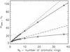 |
Fig. A.1 Number of carbon atoms nC (upper curves, diamonds) and coordination number mcoord (lower curves, triangles) for the most compact aromatic clusters possible (solid lines). The dashed lines show the simple fits to the data for general aromatic clusters. |
The coordination number per carbon atom in the aromatic cluster is plotted in Fig. A.2. In this figure the large diamonds show the values for the most compact aromatic clusters possible, i.e., for the large clusters these are the equivalent to the coronene, ovalene, circumcorenene, etc. structures. The small diamonds and their connecting dashed lines show the values for the multilinear acenes with Nrow = 1, 2, 3, 4 and 5 (from top to bottom). The small diamonds mark the actual cluster values and the dashed lines are calculated using the multilinear acene expressions (given in the middle of Table A.1). The horizontal dotted line indicates the limiting values (0.5) for simple linear acenes (Nrow = 1). Note that the compact cluster expression in the upper portion of Table A.1 is equivalent to the multilinear acene expression with Nrow = 2. The thick solid line gives a fit for the most compact aromatic clusters calculated using the expressions in the lower portion of Table A.1.
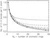 |
Fig. A.2 Ratio of the coordination number m to the number of carbon atoms nC in aromatic clusters, i.e., the maximum possible number of peripheral aromatic cluster C–H bonds per carbon atom. See the text for a full description of the plotted data. |
Appendix B: eRCN model extension possibilities
The mathematical basis of the RCN and eRCN models (e.g., Phillips 1979; Döhler et al. 1980; Thorpe 1983; Angus & Jansen 1988; Jones 1990) is a pair of equations with three inter-dependent variables, viz.,  (B.1)and
  (B.2)Solutions to these equations are found by combining or “collapsing” two of the variables into a single one, i.e., Xsp3/Xsp2 ≡ R, and solving for R as a function of XH. It is therefore evident that the addition of any new structural component into the system introduces a new variable, which renders the resulting equations unsolvable because we then have two equations and four variables. This limitation could be circumvented in several ways:
-
1.
By a collapsing of three of the variables into one, i.e.,Xsp/(Xsp3 + Xsp2) = P. However, this leads to ambiguities because of the degeneracy between the variables in the denominator and therefore to no useful or physically-realistic solutions.
-
2.
By fixing the concentration of the new component. This is a useful strategy but requires that the atomic fraction of the new component, W, is well-constrained by measurements and also that the number of involved atoms is invariant and independent of the network structure, i.e., no atomic loss, or transformation, of component W is allowed. New carbon atom hybridisation or polyatomic structures, such as sp1 C atoms or five-fold C5 aromatic rings, do not fulfil this condition and therefore cannot be treated in this way. The addition of hetero-atoms, such as O and N, should be possible using this approach, provided that their atomic abundances remain fixed. However, fixing the abundance of O and/or N atoms, and then treating their contribution as a constant, does not correctly take into account their accommodation into the structure and does not lead to realistic or useful solutions.
-
3.
By the elimination of one of the variables. For example, in order to introduce sp1 C atoms it is possible to eliminate either the Xsp3 or the Xsp2 component and then solve as a function of XH by combining the remaining two variables. However, in neither of these particular cases does this result in physically-meaningful solutions, which is not surprising since this treatment imposes unrealistic network constraints, i.e., networks consisting of only sp1 and sp2 atoms, with 2- and 3-fold coordination, or of only sp1 and sp3 atoms, with 2- and 4-fold coordination. The readers are left to verify this limitation for themselves.
In conclusion, it does not yet appear possible to add another carbon atom or hetero-atom component to the eRCN model in a physically-realistic way.
Acknowledgments
I would like to thank the referee, Walt Duley, for many valuable suggestions. This research was, in part, made possible through the financial support of the Agence National de la Recherche (ANR) through the program Cold Dust (ANR-07-BLAN-0364-01).
References
- Adel, M. E., Amir, O., Kalish, R., & Feldman, L. C. 1989, J. Appl. Phys., 66, 3248 [NASA ADS] [CrossRef] [Google Scholar]
- Angus, J. C., & Hayman, C. C. 1988, Science, 241, 913 [NASA ADS] [CrossRef] [PubMed] [Google Scholar]
- Angus, J. C., & Jansen, F. 1988, J. Vacuum Sci. Technol., 6, 1778 [Google Scholar]
- Clark, B. C., Mason, L. W., & Kissel, J. 1987, A&A, 187, 779 [NASA ADS] [Google Scholar]
- Compiègne, M., Verstraete, L., Jones, A., et al. 2011, A&A, 525, A103 [NASA ADS] [CrossRef] [EDP Sciences] [Google Scholar]
- Dadswell, G., & Duley, W. W. 1997, ApJ, 476, 184 [NASA ADS] [CrossRef] [Google Scholar]
- Dalle Ore, C. M., Fulchignoni, M., Cruikshank, D. P., et al. 2011, A&A, 533, A98 [NASA ADS] [CrossRef] [EDP Sciences] [Google Scholar]
- Dartois, E., & Muñoz-Caro, G. M. 2007, A&A, 476, 1235 [NASA ADS] [CrossRef] [EDP Sciences] [Google Scholar]
- Dartois, E., Marco, O., Muñoz-Caro, G. M., et al. 2004a, A&A, 423, 549 [NASA ADS] [CrossRef] [EDP Sciences] [Google Scholar]
- Dartois, E., Muñoz Caro, G. M., Deboffle, D., & d’Hendecourt, L. 2004b, A&A, 423, L33 [NASA ADS] [CrossRef] [EDP Sciences] [Google Scholar]
- Dartois, E., Muñoz Caro, G. M., Deboffle, D., Montagnac, G., & D’Hendecourt, L. 2005, A&A, 432, 895 [NASA ADS] [CrossRef] [EDP Sciences] [Google Scholar]
- Dischler, B., Bubenzer, A., & Koidl, P. 1983a, Solid State Commun., 48, 105 [NASA ADS] [CrossRef] [Google Scholar]
- Dischler, B., Bubenzer, A., & Koidl, P. 1983b, Appl. Phys. Lett., 42, 636 [NASA ADS] [CrossRef] [Google Scholar]
- Döhler, G. H., Dandaloff, R., & Bilz, H. 1980, J. Noncryst. Solids, 42, 87 [Google Scholar]
- Duley, W. W. 1995, ApJ, 445, 240 [NASA ADS] [CrossRef] [Google Scholar]
- Duley, W. W. 1996, MNRAS, 283, 343 [NASA ADS] [Google Scholar]
- Duley, W. W. 2000, ApJ, 528, 841 [NASA ADS] [CrossRef] [Google Scholar]
- Duley, W. W. 2001, ApJ, 553, 575 [NASA ADS] [CrossRef] [Google Scholar]
- Duley, W. W., & Williams, D. A. 2011, ApJ, 737, L44 [NASA ADS] [CrossRef] [Google Scholar]
- Duley, W. W., Seahra, S., & Williams, D. A. 1997, ApJ, 482, 866 [NASA ADS] [CrossRef] [Google Scholar]
- Duley, W. W., Grishko, V. I., Kenel, J., Lee-Dadswell, G., & Scott, A. 2005a, ApJ, 626, 933 [NASA ADS] [CrossRef] [Google Scholar]
- Duley, W. W., Lazarev, S., & Scott, A. 2005b, ApJ, 620, L135 [NASA ADS] [CrossRef] [Google Scholar]
- Ferrari, A. C., & Robertson, J. 2004, Phil. Trans. R. Soc. Lond. A, 362, 2477 [NASA ADS] [CrossRef] [Google Scholar]
- Fink, J., Müller-Heinzerling, T., Pflüger, J., et al. 1984, Phys. Rev. B, 30, 4713 [NASA ADS] [CrossRef] [Google Scholar]
- Godard, M., & Dartois, E. 2010, A&A, 519, A39 [NASA ADS] [CrossRef] [EDP Sciences] [Google Scholar]
- Godard, M., Féraud, G., Chabot, M., et al. 2011, A&A, 529, A146 [NASA ADS] [CrossRef] [EDP Sciences] [Google Scholar]
- Goto, M., Gaessler, W., Hayano, Y., et al. 2003, ApJ, 589, 419 [NASA ADS] [CrossRef] [Google Scholar]
- Goto, M., Kwok, S., Takami, H., et al. 2007, ApJ, 662, 389 [Google Scholar]
- Grishko, V. I., & Duley, W. W. 2000, ApJ, 543, L85 [NASA ADS] [CrossRef] [Google Scholar]
- Habart, E., Boulanger, F., Verstraete, L., Walmsley, C. M., & Pineau des Forêts, G. 2004, A&A, 414, 531 [NASA ADS] [CrossRef] [EDP Sciences] [Google Scholar]
- Habart, E., Abergel, A., Boulanger, F., et al. 2011, A&A, 527, A122 [NASA ADS] [CrossRef] [EDP Sciences] [Google Scholar]
- Hu, A., & Duley, W. W. 2008a, ApJ, 672, L81 [NASA ADS] [CrossRef] [Google Scholar]
- Hu, A., & Duley, W. W. 2008b, ApJ, 677, L153 [NASA ADS] [CrossRef] [Google Scholar]
- Hu, A., Alkhesho, I., & Duley, W. W. 2006, ApJ, 653, L157 [NASA ADS] [CrossRef] [Google Scholar]
- Hu, A., Griesing, S., Rybachuk, M., Lu, Q.-B., & Duley, W. W. 2007a, J. Appl. Phys., 102, 074311 [NASA ADS] [CrossRef] [Google Scholar]
- Hu, A., Lu, Q.-B., Duley, W. W., & Rybachuk, M. 2007b, J. Chem. Phys., 126, 154705 [NASA ADS] [CrossRef] [Google Scholar]
- Iida, S., Ohtaki, T., & Seki, T. 1985, in: Optical Effects in Amorphous Semiconductors, ed. P. C. Taylor, & S. G. Bishop (New York: AIP), AIP Conf. Proc., 120, 258 [Google Scholar]
- Joblin, C., D’Hendecourt, L., Leger, A., & Defourneau, D. 1994, A&A, 281, 923 [NASA ADS] [Google Scholar]
- Jones, A. P. 1990, MNRAS, 247, 305 [NASA ADS] [Google Scholar]
- Jones, A. P. 2009, in Cosmic Dust - Near and Far, ed. T. Henning, E. Grün, & J. Steinacker, ASP Conf. Ser., 414, 473 [Google Scholar]
- Jones, A. P. 2012a, A&A, 540, A2 (Paper II) [NASA ADS] [CrossRef] [EDP Sciences] [Google Scholar]
- Jones, A. P. 2012b, A&A, submitted (Paper III) [Google Scholar]
- Jones, A. P., & Nuth, J. A. 2011, A&A, 530, A44 [NASA ADS] [CrossRef] [EDP Sciences] [Google Scholar]
- Jones, A. P., Duley, W. W., & Williams, D. A. 1990, QJRAS, 31, 567 [NASA ADS] [Google Scholar]
- Kassavetis, S., Patsalas, P., Logothetidis, S., Robertson, J., & Kennou, S. 2007, Diamond & Related Materials, 16, 1813 [NASA ADS] [CrossRef] [Google Scholar]
- Le Page, V., Snow, T. P., & Bierbaum, V. M. 2009, ApJ, 704, 274 [NASA ADS] [CrossRef] [Google Scholar]
- Marée, C. H. M., Vredenberg, A. M., & Habraken, F. H. P. M. 1966, Mat. Chem. Phys., 46, 198 [Google Scholar]
- Mennella, V. 2008, ApJ, 682, L101 [NASA ADS] [CrossRef] [Google Scholar]
- Mennella, V. 2010, ApJ, 718, 867 [NASA ADS] [CrossRef] [Google Scholar]
- Mennella, V., Colangeli, L., Bussoletti, E., et al. 1995, ApJS, 100, 149 [NASA ADS] [CrossRef] [Google Scholar]
- Muñoz Caro, G. M., Matrajt, G., Dartois, E., et al. 2006, A&A, 459, 147 [NASA ADS] [CrossRef] [EDP Sciences] [Google Scholar]
- Pendleton, Y. J., & Allamandola, L. J. 2002, ApJS, 138, 75 [NASA ADS] [CrossRef] [Google Scholar]
- Petrie, S., Stranger, R., & Duley, W. W. 2003, ApJ, 594, 869 [NASA ADS] [CrossRef] [Google Scholar]
- Pety, J., Teyssier, D., Fossé, D., et al. 2005, A&A, 435, 885 [NASA ADS] [CrossRef] [EDP Sciences] [Google Scholar]
- Phillips, J. C. 1979, Phys. Rev. Lett., 42, 1151 [NASA ADS] [CrossRef] [Google Scholar]
- Pino, T., Dartois, E., Cao, A., et al. 2008, A&A, 490, 665 [CrossRef] [EDP Sciences] [Google Scholar]
- Rauls, E., & Hornekær, L. 2008, ApJ, 679, 531 [NASA ADS] [CrossRef] [Google Scholar]
- Ristein, J., Stief, R. T., Ley, L., & Beyer, W. 1998, J. Appl. Phys., 84, 3836 [NASA ADS] [CrossRef] [Google Scholar]
- Robertson, J. 1986, Adv. Phys., 35, 317 [NASA ADS] [CrossRef] [Google Scholar]
- Robertson, J. 1988, Philosophical Magazine Lett., 57, 143 [Google Scholar]
- Robertson, J. 1991, Prog. Solid State Chem., 21, 199 [CrossRef] [Google Scholar]
- Robertson, J., & O’Reilly, E. P. 1987, Phys. Rev. B, 35, 2946 [NASA ADS] [CrossRef] [EDP Sciences] [Google Scholar]
- Scott, A., & Duley, W. W. 1996, ApJ, 472, L123 [NASA ADS] [CrossRef] [Google Scholar]
- Scott, A. D., Duley, W. W., & Jahani, H. R. 1997, ApJ, 490, L175 [NASA ADS] [CrossRef] [Google Scholar]
- Serra Díaz-Cano, L., & Jones, A. P. 2008, A&A, 492, 127 [NASA ADS] [CrossRef] [EDP Sciences] [Google Scholar]
- Sloan, G. C., Jura, M., Duley, W. W., et al. 2007, ApJ, 664, 1144 [NASA ADS] [CrossRef] [Google Scholar]
- Smith, F. W. 1984, J. Appl. Phys., 55, 764 [NASA ADS] [CrossRef] [Google Scholar]
- Stauffer, D., & Aharony, A. 1994, Introduction to percolation theory, revised second edn. (CRC Press) [Google Scholar]
- Sugai, H., Yoshida, S., & Toyoda, H. 1989, Appl. Phys. Lett., 54, 1412 [NASA ADS] [CrossRef] [Google Scholar]
- Tamor, M. A., & Wu, C. H. 1990, J. Appl. Phys., 67, 1007 [NASA ADS] [CrossRef] [Google Scholar]
- Thorpe, M. 1983, J. Non Crystalline Solids, 57, 355 [Google Scholar]
- Verstraete, L., Pech, C., Moutou, C., et al. 2001, A&A, 372, 981 [NASA ADS] [CrossRef] [EDP Sciences] [Google Scholar]
- Wexler, A. 1967, Appl. Spectrosc. Rev., 1, 29 [Google Scholar]
All Tables
Adopted C-H and C-C band modes in eRCN bulk materials: band centre (ν0), width (δ) and integrated cross-section (σ).
All Figures
|
Fig. 1 Carbon atom ratio R as a function of XH. Dotted line: basic RCN model (Eq. (7)), short-dashed-dotted line: C2sp2 clusters (Eq. (14)), long-dashed line: all sp2 carbon atoms in C6 aromatic clusters (Eq. (35)) and solid line: multi-C6 ring aromatic clusters (Eq. (40)) and methyl groups (Eq. (52)). The upper and flatter solid lines show the mean atomic coordination number, |
| In the text | |
|
Fig. 2 R as a function of XH for the best-fit RCN model (Eq. (52), lower solid red line) and DG model (with L = 2, Eq. (75), lower dashed red line); the corresponding values of mC for each model are shown in the upper “flatter” red lines. Shaded: validity-ranges for the RCN (right) and DG (left) models, darker where they overlap. Thick dash-dotted: mean number of rings per aromatic cluster (NR/10). Thin dash-dotted: mean number of C atoms per aromatic cluster (nC/20). Short dashed: aromatic domain size (da in nm). Long-dashed: aromatic coherence length (La in nm). Diamonds; laboratory data for R (Angus & Jansen 1988, and references therein). |
| In the text | |
|
Fig. 3 The CH2/CH3 abundance ratio as a function of XH for the aliphatic carbon component in the best-fit eRCN model (Eq. (52)). |
| In the text | |
|
Fig. 4 The aromatic, fXsp2 (red), olefinic, (1 − f)Xsp2 (orange), total sp2, Xsp2 (grey dashed), aliphatic, Xsp3 (blue) and CH3, φXsp3 (black dashed), carbon atom fractions as a function of XH for the best-fit eRCN model (Eq. (52)). |
| In the text | |
|
Fig. 5 As for Fig. 4 with the aromatic ( |
| In the text | |
|
Fig. 6 The fraction of all carbon atoms (XC,noH(total), green), sp2 aromatic (Xsp2,ar,noH, red), olefinic (Xsp2,noH, orange) and sp3 (Xsp3,noH, blue) carbon atoms as a function of XH that are not attached to a hydrogen atom, for the best-fit eRCN model (Eq. (52)). |
| In the text | |
|
Fig. 7 The adopted wavelength-dependent, IR band cross-sections per carbon atom, σC (1 Mb = 10-18 cm2), for the eRCN model as a function of XH ( ≡ Eg). The upper curves (purple) are for the H-rich, wide band gap materials and the cross-sections, in the 8 μm region, decrease with decreasing XH from top to bottom – XH = 0.58 (purple), 0.52 (cobalt), 0.46 (blue), 0.40 (green), 0.34 (yellow), 0.29 (orange), 0.23 (brown) and 0.17 (red). |
| In the text | |
|
Fig. 8 The predicted eRCN spectrum in the 3.2−3.6 μm C-H stretching region as a function of XH calculated using the structural de-composition described in Sect. 2.2.3 and the data in Table 2. The diamonds, squares and triangles indicate the aliphatic, olefinic and aromatic band positions, respectively (see Table 2). The data with error bars are for the diffuse ISM absorption along the Galactic Centre IRS6E line of sight (black) and Cyg OB2 No. 12 (grey) (taken from Pendleton & Allamandola 2002). |
| In the text | |
|
Fig. 9 The predicted eRCN spectrum in the 6.0−7.5 μm C-H bending and C-C mode region as a function of XH calculated using the structural de-composition described in Sect. 2.2.3 and the data in Table 2. The symbols are the same as for the previous figure. The grey shaded areas indicate the approximate full width of the observed a-C:H bands in this region (e.g., Pendleton & Allamandola 2002; Dartois et al. 2005). |
| In the text | |
|
Fig. 10 The predicted full eRCN spectrum in the 3−8 μm C-H stretching and bending and C-C mode region as a function of XH calculated using the structural de-composition described in Sect. 2.2.3 and the data in Table 2. Here the spectra are normalised to the strongest band for each value of XH. The data with error bars and the shaded areas indicate the diffuse ISM bands as per Figs. 8 and 9. |
| In the text | |
|
Fig. 11 The predicted full DG spectrum in the 3−8 μm C-H stretching and bending and C-C mode region as a function of XH calculated using the structural de-composition described in Sect. 2.2.3 and the data in Table 2. Here the spectra are normalised to the strongest band for each value of XH. On the left the strongest bands are for high XH > 0 (green to brown), while the opposite is true for the longer wavelength bands on the right (shortward of 6.8 μm). The data with error bars and the shaded areas indicate the diffuse ISM bands as per Figs. 8 and 9. |
| In the text | |
|
Fig. 12 The defected graphite (DG) network model. The filled (open) circles represent carbon (hydrogen) atoms in an aromatic network. The inset dotted circles indicate rings with aromatic character. |
| In the text | |
|
Fig. 13 The predicted eRCN and DG spectra, presented as the absorption coefficient, α, in the 2.5 − 13.5 μm region as a function of Eg calculated using the structural de-composition described in Sects. 2.2.3, 2.2.4 and 2.3 and for the data in Table 2. The adopted colour-coding for this plot is from large band gap (2.67 eV, purple) to low band gap (–0.1 eV, black) with intermediate values in steps of 0.25 eV from 2.5 (violet) to 0 eV (grey) with the addition of the Eg = 0.1 and − 0.1 eV cases (light grey and black, respectively), as per Paper II. The bands with central positions long-ward of the vertical grey line (λ(ν0) > 7.3 μm) are not yet well-determined by laboratory measurements. |
| In the text | |
|
Fig. A.1 Number of carbon atoms nC (upper curves, diamonds) and coordination number mcoord (lower curves, triangles) for the most compact aromatic clusters possible (solid lines). The dashed lines show the simple fits to the data for general aromatic clusters. |
| In the text | |
|
Fig. A.2 Ratio of the coordination number m to the number of carbon atoms nC in aromatic clusters, i.e., the maximum possible number of peripheral aromatic cluster C–H bonds per carbon atom. See the text for a full description of the plotted data. |
| In the text | |
Current usage metrics show cumulative count of Article Views (full-text article views including HTML views, PDF and ePub downloads, according to the available data) and Abstracts Views on Vision4Press platform.
Data correspond to usage on the plateform after 2015. The current usage metrics is available 48-96 hours after online publication and is updated daily on week days.
Initial download of the metrics may take a while.