| Issue |
A&A
Volume 539, March 2012
|
|
|---|---|---|
| Article Number | A131 | |
| Number of page(s) | 15 | |
| Section | The Sun | |
| DOI | https://doi.org/10.1051/0004-6361/201117675 | |
| Published online | 06 March 2012 | |
An active region filament studied simultaneously in the chromosphere and photosphere
I. Magnetic structure
1
Instituto de Astrofísica de Canarias,
vía Láctea s/n, 38205
La Laguna, Tenerife
Spain
e-mail: This email address is being protected from spambots. You need JavaScript enabled to view it.
2
Departamento de Astrofísica, Universidad de La
Laguna, 38206 La
Laguna, Tenerife,
Spain
3
High Altitude Observatory (NCAR), Boulder, CO
80301,
USA
Received: 9 July 2011
Accepted: 2 December 2011
Abstract
Aims. A thorough multiwavelength, multiheight study of the vector magnetic field in a compact active region filament (NOAA 10781) on 2005 July 3 and 5 is presented. We suggest an evolutionary scenario for this filament.
Methods. Two different inversion codes were used to analyze the full Stokes vectors acquired with the Tenerife Infrared Polarimeter (TIP-II) in a spectral range that comprises the chromospheric He i 10 830 Å multiplet and the photospheric Si i 10 827 Å line. In addition, we used SOHO/MDI magnetograms, as well as BBSO and TRACE images, to study the evolution of the filament and its active region (AR). High-resolution images of the Dutch Open Telescope were also used.
Results. An active region filament (formed before our observing run) was detected in the chromospheric helium absorption images on July 3. The chromospheric vector magnetic field in this portion of the filament was strongly sheared (parallel to the filament axis), whereas the photospheric field lines underneath had an inverse polarity configuration. From July 3 to July 5, an opening and closing of the polarities on either side of the polarity inversion line (PIL) was recorded, resembling the recently discovered process of the sliding door effect seen by Hinode. This is confirmed with both TIP-II and SOHO/MDI data. During this time, a newly created region that contained pores and orphan penumbrae at the PIL was observed. On July 5, a normal polarity configuration was inferred from the chromospheric spectra, while strongly sheared field lines aligned with the PIL were found in the photosphere. In this same data set, the spine of the filament is also observed in a different portion of the field of view and is clearly mapped by the silicon line core.
Conclusions. The inferred vector magnetic fields of the filament suggest a flux rope topology. Furthermore, the observations indicate that the filament is divided in two parts, one which lies in the chromosphere and another one that stays trapped in the photosphere. Therefore, only the top of the helical structure is seen by the helium lines. The pores and orphan penumbrae at the PIL appear to be the photospheric counterpart of the extremely low-lying filament. We suggest that orphan penumbrae are formed in very narrow PILs of compact ARs and are the photospheric manifestation of flux ropes in the photosphere.
Key words: Sun: filaments, prominences / Sun: chromosphere / Sun: photosphere / Sun: magnetic topology / techniques: polarimetric
© ESO, 2012
1. Introduction
Solar filaments, also called prominences when observed in emission outside the disk, are elongated structures formed of dense plasma, which lies above polarity inversion lines (PILs) of the photospheric magnetic field (Babcock & Babcock 1955) and has a lower temperature than its surroundings. A functional definition of the PIL would be an imaginary line that separates two close areas of opposite polarity. On disk filaments are readily identifiable in the quiet Sun (quiescent filaments) and in active regions (active region filaments) when observed using common chromospheric wavelengths, e.g., the He i 10 830 Å multiplet and the Hα 6563 Å line. The magnetic field plays a major role in their formation, stability, and evolution. As a result, spectropolarimetric observations at different heights of the atmosphere combined with high angular resolution images are needed to obtain an overall picture of the physical processes that take place in filaments. The magnetic field strength and its orientation can be inferred using appropriate diagnostic techniques that are able to interpret the Zeeman effect, as well as scattering polarization and its modification through the Hanle effect (Tandberg-Hanssen 1995, and references therein). Although many line-of-sight (LOS) observations have been carried out in the past decades, it is important to emphasize the need for full-Stokes measurements in order to have complete information of the vector magnetic field.
According to observational studies, the magnetic field topology under active region (AR) filaments has sheared or twisted field lines along the PIL that can support dense plasma in magnetic dips (Lites 2005; López Ariste et al. 2006). Previous findings about prominence magnetic structure have shown models with dipped field lines in a normal (Kippenhahn & Schlüter 1957) or inverse1 (Kuperus & Raadu 1974; Pneuman 1983) polarity configuration, the latter having a helical structure. From a large sample of quiescent prominence observations, Leroy et al. (1984) found both types of configurations and a strong correlation between the magnetic field topology and the height of the prominence. On the other hand, Bommier et al. (1994) found predominantly inverse polarity configurations. However, more recent photospheric spectropolarimetric observations of AR filaments have revealed that both configurations can coexist in the same filament (Guo et al. 2010) or even evolve with time from one type to the other, as presented by Okamoto et al. (2008) from the analysis of vector magnetogram sequences.
The formation process of filaments is still a controversial issue in solar physics, so it has been widely debated. On the one hand, there is the sheared arcade model that, by large-scale photospheric footpoint motions (such as shear at, and convergence towards the PIL, and subsequent reconnection processes), is able to form dips and even helical structures, where plasma can be gravitationally confined (e.g., Pneuman 1983; van Ballegooijen & Martens 1989; Antiochos et al. 1994; Aulanier & Demoulin 1998; DeVore & Antiochos 2000; Martens & Zwaan 2001; Welsch et al. 2005; Karpen 2007). This model is capable of reproducing both inverse and normal polarity configurations in the same filament (Aulanier et al. 2002). However, recent observational works in a quiescent filament (Hindman et al. 2006) and along an AR filament channel (Lites et al. 2010) did not find evidence of these systematic photospheric flows that converged at the PIL and triggered reconnection processes. In our opinion, more observations are needed to support this important result.
On the other hand, the flux rope emergence model assumes that the twist in the field lines is already present in the convection zone before emerging into the atmosphere (e.g., Kurokawa 1987; Low 1994; Low & Hundhausen 1995; Lites 2005). The rise of twisted magnetic fields has been studied by various authors through both observations (Lites et al. 1995, 2010; Leka et al. 1996) and three-dimensional (3D) numerical simulations (e.g., Fan 2001; Archontis et al. 2004; Magara 2004; Martínez-Sykora et al. 2008; Fan 2009; Yelles Chaouche et al. 2009). Such an emerging helical flux rope scenario, combined with the presence of granular flows, is supposedly the main process of formation and maintenance of the AR filament studied by Okamoto et al. (2008, 2009). Recent nonlinear force-free field (NLFFF) extrapolations of photospheric magnetic fields underneath AR filaments (Guo et al. 2010; Canou & Amari 2010; Jing et al. 2010) have agreed that the main structure has to be a flux rope, although Guo et al. (2010) also find dipped arcade field lines in the same filament. Flux rope emergence from below the photosphere encounters severe difficulties to reach chromospheric layers and above, since it is loaded with mass (e.g., Archontis & Török 2008). Indeed, the previous work suggests that a second flux rope formed from instabilities and atmospheric reconnection is what lifts up the mass and forms the observed active region filaments.
The main difference between the sheared arcade and the emerging flux rope models is the existence of a flux concentration stuck at photospheric levels in the latter scenario. The reader is referred to the paper of Mackay et al. (2010) for a recent review of the magnetic structure of filaments.
In the past, only a few measurements have been made of the magnetic field strength in AR filaments. For instance, Kuckein et al. (2009), using the same data set as described in this paper, find a predominance of Zeeman-like signatures in the Stokes profiles. Using three different methods, they infer very strong magnetic fields in the filament (600–700 Gauss), with a dominant transverse component (with respect to the LOS).
The aim of this paper is to study the strength and topology of the magnetic field in an active region filament at photospheric and chromospheric heights simultaneously. Recently, several studies have presented analyses of the vector magnetic field in filaments or prominences from observations either in the photosphere (e.g., Lites 2005; López Ariste et al. 2006; Okamoto et al. 2008; Guo et al. 2010; Lites et al. 2010) or the chromosphere (e.g., Lin et al. 1998; Casini et al. 2003; Merenda et al. 2006; Kuckein et al. 2009), but none of them have inferred the field at both heights at the same time. The 10 830 Å spectral region, which includes a chromospheric He i triplet and a photospheric Si i line, offers a unique spectral window to understanding the physical processes that take place in AR filaments as already shown by Sasso et al. (2011). In this work, we focus on the overall magnetic configuration observed simultaneously in the photosphere and the chromosphere.
2. Observations
The active region filament, NOAA AR 10781, was observed on 2005 July 3 and 5 using the Tenerife Infrared Polarimeter (TIP-II, Collados et al. 2007) at the German Vacuum Tower Telescope (VTT, Tenerife, Spain). TIP-II acquires images at four different modulation states and combines them in order to measure the Stokes parameters (I, Q, U, and V) along the spectrograph slit.
The latitude and longitude of the filament region was N16-E8 (around μ ~ 0.95) for the first day, and N16-W18 (μ ~ 0.91) for the second. During the observations, real time Hα images and SOHO/MDI (Scherrer et al. 1995) magnetograms were used as a reference to position the slit (0 5 wide and 35′′ long) at the center of the AR, on top of the polarity inversion line. Figure 1 shows two Big Bear Hα images from July 1 and 5 where the filament can easily be recognized. On July 1, the filament shows a more diffusive nature than on July 5, when it displays a rather compact configuration with brighter Hα emission from the plage flanking it. Scans were taken with TIP-II from E to W with the slit parallel to the PIL and step sizes of 04 for July 3 and 03 for July 5, making up at least a field of view (FOV) of ~30″ × 35″, with a pixel size along the slit of 017.
The TIP-II spectral range spanned from 10 825 to 10 836 Å with an original spectral sampling of ~11.04 mÅ px-1. This spectral window included the photospheric Si i line at 10 827 Å and the chromospheric He i triplet at 10 830 Å. It also contained at least one telluric H2O line, which was used for the absolute velocity calibration.
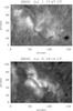 |
Fig. 1 Big Bear Hα image of the active region under study. The leader sunspot is seen in the bottom right corner. The filament is seen on both days, July 1 and 5. Note the more compact nature of the plage emission on the second day. |
All images were corrected for flat field and dark current and was calibrated polarimetrically following standard procedures (Collados 1999, 2003). The adaptive optics system of the VTT (KAOS, von der Lühe et al. 2003) was locked on nearby pores and orphan penumbrae, i.e., penumbral-like structures not connected to any umbra (a term coined by Zirin & Wang 1991), and highly improved the observations that had changeable seeing conditions. A binning of 3 px in the spectral domain, 6 px along the slit, and 3 px along the scanning direction was carried out to improve the signal-to-noise ratio needed for the full Stokes spectral line inversions. Thus, the final spectral sampling was ~33.1 mÅ px-1. The spatial resolution, when the KAOS system was locked, reached ~1′′. However, the binned data used for the inversions (except when stated otherwise) had a resolution of 2′′.
The He i triplet comprises three spectral lines, which according to the National Institute of Standards and Technology (NIST), are the 10 829.09 Å “blue” component and the “red” components at 10 830.25 Å and 10 830.34 Å lines. The last two are blended and consequently appear as a single spectral line in the solar spectrum. The formation height of the helium triplet happens in the upper chromosphere (Avrett et al. 1994), so it is especially interesting for the study of filaments and their magnetic properties, as already proved by many authors (Lin et al. 1998; Trujillo Bueno et al. 2002; Merenda et al. 2007; Casini et al. 2009; Kuckein et al. 2009; Sasso et al. 2011). The strong photospheric Si i absorption line at 10 827.089 Å originates between the terms  and has a Landé factor of geff = 1.5. The combination of these lines is an excellent diagnostic tool for studying magnetic fields and their coupling between the photosphere and the chromosphere.
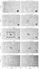 |
Fig. 2 Time sequence of SOHO/MDI continuum images of the whole active region NOAA 10781 between July 2 and 6 of 2005. The black box shows the size and location of the maps of Fig. 3, which have a smaller but more detailed FOV. A developed sunspot can be seen at the bottom right corner of the AR. Between July 2 and 3 the center of the AR was almost devoid of pores. On July 5 we increased the cadence of the sequence in order to show the quick appearance of new pores and orphan penumbrae at the PIL during that day. |
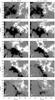 |
Fig. 3 SOHO/MDI line-of-sight magnetogram evolution of the compact plage between July 1 and 7 of 2005. Note that the date and time of each panel does not correspond to the panels in Fig. 2. Images are saturated at ± 400 G. Solar north and west correspond to up and right, respectively. The black boxes show the approximate scanned area of TIP-II for both days. On July 3, the space between both polarities broadens in the lower part of the PIL, whereas in the following days the whole AR is more compact. The size of the panels corresponds to the black rectangle in Fig. 2. White arrows indicate the direction to disk center. |
In this paper we also report on SOHO/MDI images that are used to understand the long-term (days) evolution of the AR in the PIL region.
2.1. Evolution of the AR (SOHO/MDI)
Active region NOAA 10781 emerged some weeks before our observing run on the rear side of the Sun. Its magnetic configuration, as seen by SOHO/MDI (see below), clearly corresponds to that of an AR that is in its decay phase, i.e., a round leader sunspot followed by facular regions of both polarities that show the latitudinal shear produced by the action of surface flows (e.g., van Ballegooijen 2008). The filament is found above the PIL in the plage region. The time sequence of continuum images of MDI between 2005 July 2 and 6 is presented in Fig. 2. Since filaments are not visible here, we expanded the FOV in order to use the AR leader sunspot, located in the lower righthand corner, as a reference. As shown in Fig. 2, it is not until July 4 that small pores start to emerge and gather together. White light images of the Transition Region and Coronal Explorer (TRACE) confirm this behavior. On July 5, we increased the cadence in Fig. 2 to show that more pores quickly emerged and orphan penumbrae formed (see black rectangle on the July 5 06:24 UT panel). Interestingly, these orphan penumbral regions act like a bridge connecting different small groups of pores together. However, during July 6 the pores and orphan penumbrae disappear completely. It is also worth noting that the leading sunspot of the AR, which on July 2 had a round and rather symmetric shape, also decays away slowly over this period of time and almost vanishes by the end of July 6.
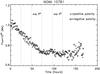 |
Fig. 4 Flux history curves for the positive (+ ) and negative (⋄ ) polarities of AR 10781. 24-h days are separated by the vertical dotted lines. |
Figure 3 provides LOS magnetograms from MDI starting on 2005 July 1 until July 7. This period was chosen in order to carry out a detailed study of the magnetic morphology and evolution of the AR. The FOV is smaller and the panels show different dates and times than Fig. 2. The AR and its PIL are well defined. The top left image shows the two polarity regions as of July 1. On the second day, the AR became more compact and the gray area in between the two opposite polarities, i.e. the PIL, developed a winding shape that pointed approximately in the N-S direction. The next two images (from July 3) show the AR becoming even more compact, since the black and white polarities approached each other. It is important to stress that, on this day, the AR rotated counterclockwise and the PIL oriented itself at ~45° with respect to solar north. These images also reveal that from July 2 to 3, although the whole AR became more compact, the lower-right part of the PIL first broadened, then become narrower again on the next day (a process that is also seen on the upper-left part of the PIL one day later). By July 5, the PIL was highly compact with the two polarities in close contact in the scaling of the figure (± 400 G). This behavior is consistent with the observations of Okamoto et al. (2008), who describe the opening and closing of the PIL region under an AR filament as a “sliding door”. The authors found observational evidence for the emergence of a flux rope under that AR filament.
2.2. Magnetic flux evolution of the AR
Recently, the study of AR filaments has been put in the context of the global flux history of the active region as a whole (van Ballegooijen & Mackay 2007). The seminal work of van Ballegooijen & Martens (1989) showed that flux ropes (and filaments) can be formed through successive cancellations at the PIL, transforming active region flux into flux rope field lines. This process submerges as much flux below the surface as is injected into the flux rope itself. Thus, evaluating the flux losses that occur during the last stages of an active region is important for understanding this evolutionary phase. Measurements of such flux losses in an active region by Sterling et al. (2010) yielded 2.8 × 10²¹ Mx day-1. More recently, for a medium sized active region, Green et al. (2011) quoted a lower rate of 2.5 × 10²⁰ Mx day-1. This number agrees better with the estimate by Dalda & Martinez Pillet (2008), who find 4.8 × 10²⁰ Mx day-1. The latter authors also report on a clear relation between the cancellation events at the PIL and an outward-directed coronal activity, but they caution that the contribution of the cancellation events was four times less than the global flux decay rate. According to this study, not all flux losses could have been attributed to cancellations at the PIL, with the resolution and sensitivity of SOHO/MDI magnetograms.
Figure 4 displays the flux history curves for the positive and negative polarities of this active region. The two days when TIP-II observations were taken are highlighted in the figure. The active region boundaries were visually selected for each SOHO/MDI map and adapted to the size changes of the AR created by the well-known flux transport processes. The magnetic flux of each pixel is multiplied by a factor 1/cos2(θ), where θ is the heliocentric angle, to account for the LOS projection of the magnetic field (which is assumed to be vertical) and the projection effect on the pixel area. The positive flux of the active region is computed by adding the contribution of all the pixels whose flux is larger than −30 G (before multiplying by the above factor). Similarly, the negative flux of the active region is computed by adding all the pixels with fluxes below + 30 G. By including pixels with fluxes in the range [–30, +30] G (which represents the peak-to-peak noise) in the computations, we ensure efficient noise cancellation. The two polarities coincide nicely in magnitude and show a similar evolution. A linear decay phase is observed during the first three days. The flux decay rate is 9.3 × 10²⁰ Mx day-1, which is intermediate in the range of values mentioned above. We do not pursue in this work whether this could have contributed to the formation of the flux rope. Magnetic-field extrapolations of some form would be needed to conduct such a study, and this is beyond the scope of this paper. After 30% of the observed initial flux is lost, the flux curves show a plateau region where no more net losses or gains are seen. The 30% fractional decrease is, of course, a lower limit since we do not observe the onset of the decay phase. This plateau region was also encountered by Dalda & Martinez Pillet (2008); however, in their study, the amount of flux lost was found to be in the range of 50−70% of the initial value.
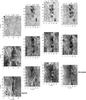 |
Fig. 5 From left to right slit-reconstructed images from the Tenerife Infrared Polarimeter (TIP-II) at different times. From top to bottom several wavelengths are presented that represent different layers in the atmosphere, from the photosphere to the chromosphere: continuum, Si i 10 827 Å line center and He i 10 830 Å red core intensities. The panels are located at different positions to approximately represent the alignment of their respective FOVs. The small white arrows indicate the position of the Stokes profiles presented in Figs. 7–9. |
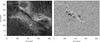 |
Fig. 6 Hα line core (left) and continuum (right) images from the Dutch Open Telescope taken on 2005 July 5th at 8:44 UT. The contour of the filament is superimposed upon the continuum image and shows that it partially lies on top of the orphan penumbrae, between the pores. In the left panel, the dashed white box indicates the approximate FOV of TIP-II for that day. |
The sliding door phenomenon was seen to occur on July 3. This date sits in the linear decay phase of the AR. However, this phase was already taking place before, and no particular slope change is seen on July 3. The appearance of the orphan penumbrae structures happens on July 4 and 5, coinciding with the flat section of the flux curve. Clearly, these processes (sliding door and orphan-penumbrae generation) cause a minimal impact on the flux curves. One way to explain this result would require that the amount of longitudinal flux change involved in both processes were at, or below, the noise level of the data (±0.3 × 10²¹ Mx).
2.3. TIP-II observations
The first set of spatial scans were taken on 2005 July 3, centered on the filament. Two maps with a FOV of 36″ × 35″, which was unfortunately not large enough to cover the whole active region (see Fig. 3), were acquired with TIP-II between 13:53 and 15:01 UT. The filament is seen all along the vertical direction. Slit-reconstructed maps at different wavelengths for one of the two data sets for this day are presented in the first column of Fig. 5. The frames in this figure are located at different positions to approximately represent the alignment of their respective FOVs. The bottom lefthand panel shows a tight filament spine, inferred from the strong He i absorption, which extends along the vertical direction. There are no big pores, but only some small magnetic features (dark patches) seen among the granulation in the continuum image on the top left panel of the figure. The Si i line core image (in the middle row) shows dark areas with larger absorption in regions of weak longitudinal field. This line weakens in faculae, as do most photospheric lines.
The second set of spectropolarimetric data was taken on July 5 between 7:36 and 14:51 UT, Cols. 2–4 in Fig. 5. Each scan took around 20 min to complete. The acquired maps were centered on a highly interesting area with very tight opposite polarities that corresponded, in continuum image, to pores and orphan penumbrae, all located along the PIL. Note that these maps overlap with the upper half of the former map from July 3 (see black boxes in Fig. 3 to get a better notion of the FOV). The He i red core intensity images in the bottom row of Fig. 5 still show the spine of the filament in the lower part. Moreover, the filament in the upper part appears to be more diffused and extended. One can easily distinguish dark helium threads formed on July 5 especially in the lower righthand panel of Fig. 5. Many authors have observed the presence of threads in filaments and prominences before (e.g., Menzel & Wolbach 1960; Engvold 1976; Lin et al. 2005, 2008; Okamoto et al. 2007). It is generally believed that dark thin features in the chromosphere near ARs trace magnetic field lines. This idea is particularly interesting when applied to threads seen in AR filaments, since it could explain the presence of magnetic dips where plasma is trapped. Nevertheless, care must be taken, since a recent paper by de La Cruz Rodríguez & Socas-Navarro (2011) proves that chromospheric fibrils mostly, but not always, trace magnetic field lines. From our maps we see that the threads observed with TIP-II change only slightly in a time range of five to six hours. This becomes apparent when closely comparing the helium maps of Cols. 2 and 4 in Fig. 5. The most prominent He i threads are located above pores or orphan penumbrae. A more detailed study of the magnetic configuration of these threads is presented below in Sect. 4.2.
Strong absorption in the Si i line core is present below the spine of the filament on July 5 (see Fig. 5). It is remarkable that the axis of the filament seems to lay so low in the atmosphere that even the highest layers of the photospheric silicon absorption line (at the core of the line) trace it.
2.4. DOT observations
High-resolution (0071/px) Hα 6563 Å images from the Dutch Open Telescope (DOT; Rutten et al. 2004) for the morning of 2005 July 5 confirm the presence of the filament, which has an inverse S-like shape and a spine in its lower part. This is also confirmed by inspection of TRACE at 171 Å images. Such an inverse S-like shape is likely to be expected in the northern hemisphere (Pevtsov et al. 2001). The lefthand panel of Fig. 6 shows one image of the Hα data set taken by the DOT at 8:44 UT. The filament is surrounded by a bright plage. The image reveals small arch-like structures in the upper half of the filament that are almost perpendicular to its axis and then, in the spine, stretch along it towards its center. These archs can be identified as the Hα counterpart of the He i threads mentioned before. A continuum image (with a 3 Å bandpass) is shown in the righthand panel of Fig. 6. This image is spatially aligned with the Hα panel on the left and has, superimposed on it in white, the Hα-contour of the filament. It is clear that the broader part of the filament lies on top of the orphan penumbrae, in between the pores, whereas the spine in the lower part is only surrounded by weaker magnetic features (small gray patches in the continuum image).
3. Spectral line inversion and data analysis
The average signal-to-noise ratio after binning the data is about 2000. Since the polarization signals of the Si i 10 827 Å line are much stronger than those of the He i triplet, it is not necessary to apply the same binning to the Si i Stokes profiles and suffer the corresponding loss of spatial resolution. However, for a better comparison between them we use the same binning criterion for both, unless stated otherwise. Two different inversion codes were used to fit the observed Stokes profiles. Both use a nonlinear least-squares Levenberg-Marquard algorithm to minimize the differences between the observed and synthetic spectra. For the He i 10 830 Å triplet a Milne–Eddington (ME) inversion code (MELANIE; Socas-Navarro 2001) that computes the Zeeman-induced Stokes spectra in the incomplete Paschen-Back (IPB) effect regime was used (see Socas-Navarro et al. 2004, for a detailed study of the effects of the IPB in the He i multiplet). MELANIE does not take the atomic-level polarization due to anisotropic radiation pumping and its modification via the Hanle effect into account. Nevertheless, by comparing the output of three different techniques with different levels of physical complexity, Kuckein et al. (2009) show that the polarization signals in this AR filament are dominated by the Zeeman effect, a fact that was supported by the excellent performance of the MELANIE inversions. This code normally uses a set of eleven free parameters, which are modified to obtain the best fits to the observed Stokes profiles: magnetic field strength (B), inclination (γ), azimuth (φ), line strength (η0), Doppler width (ΔλD), a damping parameter, LOS velocity (vLOS), the source function at τ = 0 and its gradient, macroturbulence factor and stray-light fraction (α = 1 − f), where f is the filling factor – or fraction of the magnetic component that occupies the resolution element. MELANIE requires an initial guess for the free parameters. For this purpose we carried out a magnetograph analysis and a Gaussian fit to Stokes I to obtain rough estimates for B, γ, φ, ΔλD and vLOS for each point along the slit.
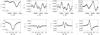 |
Fig. 7 Stokes profiles of the He i 10 830 Å triplet (four top panels) and the Si i 10 827 Å line (four bottom panels) at coordinates x ~ 20′′ and |

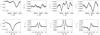 |
Fig. 8 Same as Fig. 7 but for coordinates x ~ 17′′ and y ~ 7′′ in Fig. 5, on July 5, 9:33–9:52 UT column (see white arrows pointing from left to right). These profiles belong to the spine of the filament. The magnetic field obtained from this particular fit for helium was BHe = 788 ± 11 G, γHe = 95.0° ± 0.2°, and φHe = 54.3° ± 1.1° and for silicon BSi = 1058 ± 26 G, γSi = 99.5° ± 0.8°, and φSi = 32.2° ± 1.5° with a f ~ 0.8. |
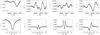 |
Fig. 9 Same as Fig. 7 but for coordinates x ~ 16′′ and y ~ 12′′, see white arrows in Fig. 5 (arrow pointing from right to left), 11, and 12, on July 5, 9:33–9:52 UT map. The Stokes profiles were observed at the polarity inversion line. The fitted parameters for the helium are BHe = 878 ± 11 G, γHe = 109.8° ± 0.3°, and φHe = 76.2° ± 1.8° and for the SIR case are BSi = 806 ± 21 G, γSi = 99.9° ± 0.8°, φSi = 56.1° ± 1.2°, and a photospheric filling factor of f ~ 0.8. |
For the thermodynamical parameters, several inversions of a few representative cases with random initial values, but within reasonable boundaries, were carried out. Averages of the retrieved parameters were calculated and used as initial guesses for the rest of the inversions.
Test inversions were carried out, where α was left as a free parameter, to control the fraction of a given nonmagnetic stray-light profile in the inversions. The results yielded almost no changes in the retrieved inclinations, azimuths, and LOS velocities. The inferred magnetic field strengths were greater than in the case without stray-light, but never by more than 100 G. Therefore, we finally decided to fix this parameter for the He i ME inversions, setting the filling factor to 1 (i.e., α = 0). The macroturbulence factor was also fixed to the calculated theoretical value of the spectral resolution of the data – a combination of slit, grating, and pixel resolution, which yielded 1.2 km s-1. Thus, only nine free parameters were left in the MELANIE fit.
The photospheric Si i 10 827 Å line was inverted using the SIR inversion code (Ruiz Cobo & del Toro Iniesta 1992) which is based on spectral line response functions (RFs) and assumes local thermodynamical equilibrium (LTE) and hydrostatic equilibrium to solve the radiative transfer equation. The advantage of using the SIR code is that a depth-dependent stratification of the physical parameters can be obtained as a function of the logarithm of the LOS continuum optical depth at 5000 Å (log τ).
We tested the effects on the inversions of using different initial model atmospheres (umbra, penumbra, and plage models), to asses their performance when reproducing the observed Stokes profiles. The penumbral model from del Toro Iniesta et al. (1994) seemed to yield the best results, which is consistent with what we see in the observations at the photosphere. However, some modifications to the model (such as assuming an initial constant magnetic field strength of 500 G and a LOS velocity of 0.1 km s-1) had to be implemented.
Different initial values for the inclination and azimuth did not affect the final fit to the observed Stokes profiles. Macroturbulence was fixed to the same value as for the ME inversions. However, for the inversion of the Si i line, the stray-light was initialized with 30% and left as a free parameter in the fit. Stray-light profiles for each map were computed by averaging the Stokes I of nonmagnetic areas, i.e., regions where Stokes Q, U, and V are negligible. The necessary atomic data for the Si i 10 827 Å line were taken from the work of Borrero et al. (2003). In particular, the value of the logarithm of the oscillator strength times the multiplicity of the lower level that we used was log (gf) = 0.363.
To have a rough idea of the formation height of silicon in order to associate an appropriate optical depth for the inferred vector magnetic field, response functions to magnetic field perturbations at various positions near or in the filament were calculated. Our atmospheric model covers heights from 1.2 up to −4.0 (in log τ units). The highest sensitivity for both days was found to take place at log τ = −2. Thus, from this point onwards, all of the figures derived from the inversions of the Si i line are referred to this height.
Figures 7–9 show the results of the MELANIE and SIR inversions of the Stokes parameters for three different positions along the filament: one in a helium dark thread, one in the spine, and one at the PIL. Each figure is made of eight plots: in the top (bottom) row we present the He i 10 830 Å (Si i 10 827 Å) observed Stokes I, Q, U, and V profiles obtained after performing the binning and the best fit achieved by the inversion code. The exact location of the selected fits is indicated by short white arrows in Figs. 5, 11, and 12 (see the captions of the figures for a detailed explanation). MELANIE does not provide the uncertainties in the retrieved atmospheric parameters. To estimate them, we used the synthetic Stokes profiles that resulted from the best fit of the model to the data. Then, several different realizations of the noise (with an amplitude of that of the noise in the observations) were added to the synthetic Stokes profiles, which were in turn inverted again. The standard deviation computed from the spread in the values of the retrieved parameters provided the errors quoted in the captions of Figs. 7−9. The SIR inversions directly provide uncertainties that are proportional to the inverse of the response functions to changes in the physical parameters.
We found a very satisfactory performance of the ME inversion code when fitting the He i Stokes profiles. This has already been described by Kuckein et al. (2009) who found in these data a ubiquitous presence of Zeeman-like signatures (see Stokes Q and U frames in Figs. 7–9) with no apparent contribution of atomic level polarization and its modification by the Hanle effect. The presence of strong Stokes Q and U profiles is indicative of strong transverse magnetic fields in the filament. In the photospheric Si i 10 827 Å absorption line we also find strong Stokes Q and U profiles, which occasionally have larger amplitudes than the corresponding Stokes V. Consequently, a predominant horizontal field is found at photospheric heights, too.
3.1. NLTE Si I line formation
Prior to the inversions of the Si i 10 827 Å line, we studied the possible impact of nonlocal thermodynamic equilibrium (NLTE) effects in the retrieved atmospheric parameters. SIR synthesizes the Stokes profiles under the assumption of local thermodynamic equilibrium. A recent study by Bard & Carlsson (2008) report that this line can be significantly affected by NLTE conditions. The authors show that the NLTE Si i line core intensity is deeper than the analogous LTE result for two different model atmospheres: quiet sun (FALC model) and sunspot umbra models (SPOTM model). To study possible effects on our inversion results, we introduced the departure coefficients β (which are defined as the ratio between population densities in NLTE over LTE) from the above cited paper (kindly provided to us by Carlsson), into the SIR code. Inversions of a few selected cases were run with the β coefficients from these models (together with the LTE case), and the differences between the inferred magnetic field strength (B), inclination (γ), and azimuth (φ) were studied. No significant changes were found for γ and φ between the β and non-β inversions; however, the field strength presented some variations. Differences with an rms value of 100 G, in the spine, and of 150 G, in the diffuse filament region in the upper part of the maps, were found. We also studied the behavior of the LOS velocities taking the various options for the β coefficients into account. The rms changes found in the spine and in the orphan penumbrae were around 0.1 and 0.2 km s-1, respectively.
These values are low, and similar to other errors arising from photon noise or systematics from the velocity calibration. NLTE effects of the Si i 10 827 Å line are certainly non-negligible when estimating the temperature (T) stratification, which was found in our tests, but this has no impact on our purely magnetic study. In general, the temperatures above the range of log τ = −0.5 and −1.0 do depend drastically on the departure coefficients used and cannot be trusted unless a self-consistent NLTE inversion of the line is carried out. However, we emphasize that no major influence on the returned vector magnetic field and velocities was found when neglecting NLTE departure coefficients.
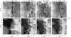 |
Fig. 10 Top: four gray-scale slit reconstructed images representing He i red core intensity, increasing with time from left to right. Superimposed are white arrows indicating the horizontal magnetic fields observed with TIP-II in the He i 10 830 Å multiplet after solving the 180° ambiguity. Especially in the top right panel the magnetic field lines are well aligned with the dark He i threads. Bottom: background images show photospheric vertical fields |
3.2. 180° ambiguity
Before transforming the vector magnetic field from the line-of-sight into the local solar frame of reference, we need to solve the well-known 180° ambiguity. Due to the angular dependence of Stokes Q and U with the azimuth, two configurations for the magnetic field, compatible with the measured Stokes profiles, are obtained, so the correct solution must be found by other means. Several methods for resolving the ambiguity in the azimuth can be found in the literature (Martin et al. 2008, and references therein). However, we were not able to apply them to our filament since the Hα high-resolution images clearly showed no barbs, and no sunspot was located immediately next to the filament to assure the continuity of the azimuth. Instead, we used the interactive IDL utility AZAM (Lites et al. 1995) to minimize the discontinuities between the two solutions of the azimuth on a pixel-by-pixel basis. Once we obtained the discontinuity-removed maps of the azimuth and the inclination in the local solar frame, we were left with two global solutions for each map, one of which needed to be rejected. In one of the two solutions the vector magnetic field pointed in the N-E direction (upward in Fig. 5), while in the other solution it pointed S-W (downward in the same figure). To select one or the other, we invoked the large-scale magnetic topology of the active region. Since our AR appeared during Solar Cycle 23 and was located in the northern hemisphere, the leader polarity must correspond to a magnetic field pointing outwards from the solar surface while the following polarity must contain a field that points inwards. In such a configuration, the toroidal field lines that created the AR necessarily had to point from W to E. If we now acknowledge that the leading polarity leans slightly towards the equator and the following polarity towards the pole (Joy’s Law), this generates a poloidal component pointing N, which corresponds to a N-E orientation of the vector magnetic field in Fig. 5 (pointing upwards) as the most probable solution.
4. Results
4.1. Vector magnetic field analysis in and underneath the filament
Average horizontal and vertical magnetic fields in each pixel were calculated using the equations given by Landi Degl’Innocenti (1992): 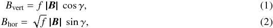 where f is the inferred filling factor, | B | the total field strength, and γ the inclination with respect to the local vertical. As mentioned in Sect. 3 we assumed f = 1 for Eqs. (1) and (2) in the case of the helium inversions. Since γ is the inclination in the local reference frame, vertical magnetic fields are radially oriented, whereas horizontal magnetic fields are parallel to the surface.
Figure 10 shows arrows denoting the horizontal magnetic field inferred from the He i triplet (upper panel) and the Si i line (lower panel) inversions after solving the 180° ambiguity for both days. Arrows are in black or white for a better distinction from the background. The gray-scale image in the top and bottom panels correspond, respectively, to a slit-reconstructed map of the He i core intensity (for the red component) and a photospheric magnetogram (saturated at ± 400 G). For July 3, the thin filament axis (or spine) lies mainly on top of the broad polarity inversion line, i.e., the gray area between opposite polarities. The photospheric vector magnetic field arrows in the lower panel depict an organized field with a predominantly inverse configuration at the PIL; i.e., the component of the transverse field perpendicular to the PIL tends to point from negative (black) to positive (white) polarity. Field vectors have, typically, a ~45° orientation clockwise with respect to the filament axis seen in the upper panel. Also, the transverse magnetic fields are stronger (longer arrows) to the right (positive polarity) than to the left (negative polarity) of the PIL. The chromospheric horizontal magnetic field presented in the upper panel appears to be highly sheared (i.e., field lines are parallel to the PIL and to the filament axis), but also displays an inverse configuration that dominates the surroundings of the spine (main axis). It is important to emphasize here that the chromospheric fields in the filament axis or spine have a stronger shear than the photospheric ones, the latter showing a preference for an inverse configuration.
The last three columns of Fig. 10 present the vector magnetic field topology of the maps of July 5 using the same criterion as described above. The spine is also seen on this day at the bottom of the panels, but the top part is dominated by a more diffuse filament in the chromosphere and by pores and orphan penumbrae in the photosphere. In all helium images (upper panels), the longest arrows, i.e., larger horizontal field component, are found in the filament between 10′′ and 22′′ on the x-axis. This also happens at photospheric layers. This readily shows that the filament area harbors the strongest horizontal fields in the region at both heights. Changes in the vector magnetic fields through the day are almost insignificant in a five to six hour time scale. Interestingly, the field lines are aligned with the dark helium threads (top panels). This can be easily seen in the last column of Fig. 10.
The inferred chromospheric field is clearly aligned with the spine (sheared configuration) in the lower part of the images and has a slightly inverse orientation close to it. This is the same behavior as observed on July 3. The photospheric fields show a predominance of the inverse configuration over the whole spine region, which again coincides with what had been observed two days earlier. In the upper part of the He i intensity images, above the spine, the chromospheric horizontal fields smoothly change orientation, displaying a normal configuration. This shift in orientation is complete in the top part of the figures, where the fields perpendicular to the PIL point straight from positive to negative polarity. The bottom panels of Fig. 10 for this day show that the photospheric horizontal fields are more aligned with the PIL, with a more sheared configuration than their chromospheric counterparts.
Thus, the filament seems to be divided in two substructures: (1) a chromospheric spine with field lines parallel to its axis and an inverse polarity configuration in the photosphere below it and (2) extensive dark helium patches or threads that show a normal polarity configuration above and, sheared field lines running along the PIL underneath, in the photosphere.
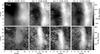 |
Fig. 11 The gray-scale images indicate the two components of the magnetic field strength inferred from the ME inversions of the He i 10 830 Å triplet. The upper/lower four panels show the vertical (Bvert)/horizontal (Bhor) fields in the local frame of reference. All images in the same row have the same intensity scale. Vertical and horizontal fields are saturated at ± 500 G and 800 G, respectively. Both polarities are close together and the PIL is only a few arcseconds wide in all panels. The white arrow indicates the location of the Stokes profiles shown in Fig. 9. |
4.2. Helium threads
We performed a more detailed study of the chromospheric He i threads, which appear in the top righthand panel of Fig. 10. The centers of two long threads are located around [x,y] = [20″,28″] and [20″,20″] , hereafter thread1 (TH1) and thread2 (TH2), respectively. They extend from just above the PIL to far into the positive polarity region. According to the orientation of the field lines, which are aligned with the threads, a normal polarity configuration pointing from positive to negative is present, and therefore it is natural to consider them as simple arches anchored in one polarity and reaching over the other. We suggest that these threads act like footpoints of the filament.
The following inferred magnetic properties are consistent with this interpretation. Along thread1, between x ∈ [18″,22″] , we found that the inclination changed from a more horizontal configuration, γTH1 ~ 66°, near the PIL to a more vertical one, γTH1 ~ 35° farther away from it, in the positive polarity plage region. An inclination of γ = 90° means that the field lines are parallel to the solar surface. Along with this, the horizontal fields decreased from  to 360 G, whereas the total field strength remained almost constant along the structure; i.e., the vertical component of the field
  increased. The same happened in thread2, between x ∈ [19″,22″] : inclinations became more vertical away from the PIL, going from γTH2 ~ 68° to 38°, while the horizontal fields decreased from
  to 360 G. These findings suggest that these threads magnetically link the chromosphere and the photosphere. The Si i data also show that the fields are more vertical near the ending points of both threads. As a consequence, the threads could constitute a channel for plasma to flow down along them. Mass flows from the filament into the photosphere through these channels will be studied in the second paper of this series.
4.3. Vertical and horizontal magnetic field components
The changes in the vertical (Bvert) and horizontal (Bhor) magnetic fields at both heights and for both days are displayed in Figs. 11 and 12. Several properties are worth mentioning.
-
1.
A comparison between Figs. 11 and 12 shows that the horizontal fields at the spine of the filament are stronger in the chromosphere than in the photosphere underneath. This is consistent throughout both days, along the spine on July 3 and outside the pores and orphan penumbrae (the lower half of the maps) on July 5. On average,
 by ~100 G.
 -
2.
Figure 11 shows that the spine in the chromosphere has a weaker horizontal magnetic field (
 400–500 Gauss) than the region above the orphan penumbrae observed on July 5, which reaches horizontal field strengths as high as 800 G (the region studied in detail by Kuckein et al. 2009).
 -
3.
The aforementioned chromospheric strong fields of July 5 are clearly related to the presence of pores and orphan penumbrae in the photosphere. The corresponding photospheric horizontal fields are the strongest there, too (see Fig. 5 for the exact location of the pores and orphan penumbrae). The observed
 in these areas is in the range of 1000–1100 G.
 -
4.
Vertical fields seem to be very similar at both heights. However,
appears to be weaker and have a more homogeneous distribution than  .
.
It is of interest to see the spatially widening and narrowing between opposite polarities. On July 3 there is a big gap (gray area of around 6′′ wide) between positive and negative polarities in the image. Interestingly, the absence of vertical fields is better seen at photospheric heights (see top left panel of Fig. 12) rather than in the chromosphere. The same widening can also be seen in the MDI LOS magnetograms (see Fig. 3; starting at the second row from the top). Two days later, on July 5, the opposite polarities have moved closer together, forming an extremely compact active region PIL. Although only the upper half map of July 3 overlaps with the lower half of July 5, the gap is undoubtedly smaller on the second day.
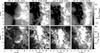 |
Fig. 12 Same as Fig. 11 but for the SIR inversions of the Si i 10 827 Å line. On July 5, the horizontal fields are concentrated at the pores (better seen when compared to Fig. 5) and reach top values of up to 1100 G. Black (negative) and white (positive) polarities of the top panels are close together, indicating a very compact AR. |
4.4. Azimuth changes between the photosphere and the chromosphere
Figure 13 analyzes the differences between the azimuths inferred from the He i (φHe) and Si i (φSi) inversions after solving the 180° ambiguity. Although only two data sets are presented, all of the other maps show very similar results. Figures 13a, b compare the photospheric and chromospheric horizontal fields for the two days. The white contours in the panels delimit the regions with predominantly horizontal magnetic fields. The adopted selection criterion defined “horizontal fields” as those having an inclination with respect to the local frame of reference in the range of 75° < γHe < 105°. Azimuth differences2, φHe − φSi, in between the white contours are presented in the histograms of Figs. 13c, e, revealing that:
-
1.
on July 3 (i.e., observing mostly the spine region) bothphotospheric and chromospheric fields seem to follow eachother, differing by only 5°–10°, with the He i arrows more aligned with the filament axis (see Fig. 13d);
-
2.
on July 5, on the other hand, it was the photospheric field that was more aligned with the PIL, and the azimuths showed a larger discrepancy, of 10°–20° on average;
-
3.
the φHe angles are systematically larger than the φSi.
To understand why the azimuth of the chromospheric vector field always pointed in a slightly counterclockwise direction with respect to the photospheric one, we provide the inset of Fig. 13d.
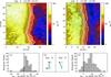 |
Fig. 13 a, b) Background color image shows the inclination angle γHe inferred from the He i inversions. Superimposed black (blue) arrows indicate the helium (silicon) horizontal fields in the local frame of reference. The white contour along the y-axis encloses horizontal fields according to the criterion of inclinations between 75° < γHe < 105°. c, e) Histogram densities of the inferred azimuth differences between helium and silicon, φHe − φSi, only for the arrows that are enclosed within the white contour in the a) and b) panels. d) Most common azimuth configurations between helium and silicon above y ~ 8 and y ~ 12, for July 3 and 5 respectively. |
On July 3, the chromospheric magnetic field was aligned with the spine, while the photospheric one displayed an inverse configuration, hence with smaller azimuth angles (angles are measured from the x-axis and increase counterclockwise). We interpret this as indicating that the field lines were wrapped around the filament axis. On July 5, the situation was reversed: the filament axis was delineated by the photospheric field lines, while the chromospheric ones showed a normal polarity configuration, thus mapping a higher part of the structure than two days earlier. Again the chromospheric azimuth angles were larger than the photospheric ones.
5. Discussion
This paper is an extensive study of the vector magnetic field at two different heights in a filament that lies on top of the polarity inversion line of an active region. This study is mostly based on TIP-II data in the 10 830 Å spectral region, but it also uses other multiwavelength data sources. Helium intensity core images clearly show the presence of a thin filament spine, which we identify with the filament axis, on top of the PIL on both days. Our observations reveal that this spine is dominated by strong homogeneous horizontal fields, typically in the range of 400−500 G in the chromosphere and 100 G smaller in the photosphere underneath. Vertical gradients of the field strength with stronger fields in the upper layers have already been observed (e.g., in polar crown prominences as shown by Leroy et al. 1983) and modeled in the past (Aulanier & Démoulin 2003) and been ascribed to the presence of dips (Anzer 1969; Demoulin & Priest 1989). The vector magnetic field in the filament spine at chromospheric heights is highly sheared (i.e., parallel to the PIL), while the photospheric vector field below the spine shows a uniformly inverse polarity. Such a configuration naturally suggests a flux rope topology. This scenario is also favored by the TRACE at 171 Å, which showed the filament with an inverse-S shape structure. Such a shape is thought to indicate the existence of an underlying flux rope (Gibson et al. 2002). This configuration of the spine, with inverse orientation in the photosphere and sheared field lines in the chromosphere, shows no significant change in the observed two-day interval. Evidence of the filament back on July 1 was presented in the BBSO Hα images (see Fig. 1). This readily shows that the process that created the filament occurred well before our observations. We tentatively identify this previously existing filament with the spine region in our observations, and remark on the fact that it showed almost no evolution during our observing campaign.
However, the PIL region was not inactive in this time lapse from the 3 to the 5 of July. MDI line-of-sight magnetograms show a widening (on July 3) and a narrowing (on July 5) of the opposite polarities of the AR. The photospheric longitudinal magnetic field obtained with TIP-II on July 3 also indicates a wide separation of both polarities compared to the more compact PILs observed on July 5. On this day, the FOV included not only the spine region, but also the newly appeared orphan penumbrae and pores. This region has a magnetic topology that is fundamentally different from that of the spine discussed before. The upper panels in Fig. 10 show chromospheric field lines with a normal polarity configuration (above y ~ 15′′). The horizontal fields there are stronger than in the spine, reaching up to 800 G (see Kuckein et al. 2009). This normal polarity configuration suggests there are field lines that directly connect opposite polarities. On the other hand and most noticeably, in the lower panels of Fig. 10, the photospheric field lines always point along the PIL, with a clear sheared configuration. The strengths of these PIL-aligned fields are high, in the range of 1000–1100 G. Now, the shear is seen in the photosphere, below the chromospheric arching field lines in a normal configuration. If a flux rope above the photosphere were found in the spine region, a similar flux rope would need to be sitting underneath it, at photospheric heights. A simple potential arcade model can be excluded here since no sheared field lines are expected in the photosphere for such a configuration. In the scenario that we suggest, the helium Stokes profiles would be mapping the top arching field lines with a normal configuration, while the axis of the rope, with sheared fields, would be located in the denser photosphere. The field strength of the structure is high enough to generate pore-like darkenings and penumbral alignments. Moreover, as these structures become visible following the widening and closing of the PIL region, we are tempted to suggest that what we are witnessing is the emergence to the surface of a flux rope structure. Unfortunately, the limited amount of observations at our disposal and the prevailing seeing conditions prevent a study of the evolution similar to the one by Okamoto et al. (2008, 2009). However, the simultaneous observations in the chromosphere and the photosphere that we present in this paper indicate that a similar process might be at work.
There is another subtle indication that a lower lying flux rope exists in this part of the FOV observed on July 5. As stated before, the spine region displays the same configuration on both days, in agreement with a flux rope located at chromospheric heights. However, there is one difference between the Si i absorption images on both days (see Fig. 5). While on July 3 the spine is not seen in the silicon core images, it does become obvious in those from July 5, suggesting that, in this case, the axis of the filament sits at lower heights. It is as if the proximity of the orphan penumbrae and pore region (interpreted here as a flux rope in the photosphere), forces the axis of the main filament to move to lower layers.
Recently, MacTaggart & Hood (2010) have studied the “sliding doors” effect through 3D magnetohydrodynamic (MHD) simulations. They report that this effect develops out of the emergence and expansion at the photosphere of a flux rope. In their simulations, the main axis of the flux bundle emerges, thanks to the magnetic buoyancy instability, to heights just slightly above the photosphere. For this area of the observed map (i.e., excluding the spine), we tentatively propose a scenario where an emerged flux rope is trapped (or slowly evolving) in the photosphere, as reported in the simulations of MacTaggart & Hood (2010). In this scenario, the observed pores and orphan penumbrae are the white-light counterparts of a flux rope trapped in the photosphere that is indeed part of the filament. To our knowledge, this is the first observational evidence of a trapped flux rope in the photosphere. Along with the works of Okamoto et al. (2008, 2009) and Lites et al. (2010), this work is the third example of observations of a “sliding door” and flux rope emergence scenario inside an AR filament, with almost the same time scale (~1 day).
One could argue that such an emergence process must leave a fingerprint on a flux history curve of the active region (as proposed recently by Vargas Domínguez et al. 2011). No such indication is seen in Fig. 4, neither when it emerged in the sliding door phase (on July 3), nor on July 4–5 when, at some point, the trapped flux rope emerged and generated the observed pores and orphan penumbrae system. However, it is important to point out that all these processes mainly involve transverse fields to which the longitudinal magnetograms from SOHO/MDI are blind. As long as the longitudinal flux involved in any of these events stays below the flux noise level in Fig. 4 (0.3 × 10²¹ Mx), it will remain undetectable. This can be accomplished by flux ropes that are not highly twisted (with a dominant axial flux over a poloidal component). For example, the case shown by Vargas Domínguez et al. (2011) involves a flux increase of 0.1 × 10²¹ Mx, which would be buried in the noise of our flux curves.
The filament formation model by van Ballegooijen & Martens (1989) and the model of active region evolution by van Ballegooijen & Mackay (2007) form, through successive reconnections above the photosphere, a twisted flux rope with a strong shear at the axis. The reconnection gives rise to two types of field lines: sheared field lines that form the axis of the helical rope and normally oriented loops below them (see Figs. 1 and 5 in van Ballegooijen & Martens 1989; van Ballegooijen & Mackay 2007, respectively). In these models, the photosphere acts as barrier to the submergence of sheared fields, which must stay in the corona once created by reconnection. However, the loops with a normal configuration must submerge below the photosphere and cross this layer at some point. This submergence is driven by tension forces pointing down and the involved spatial scales are small (900 km, see Fig. 1 in van Ballegooijen & Martens 1989). While these scales were not easily accessible to quantitative vector magnetograms in the past, the data presented in this paper achieve the needed resolution and can be used to search for evidence of these reconnected field lines. We did not find such a normally oriented component in our photospheric vector magnetic field maps. This is true not only for the inversions done with binned data, but also for the inversions done of the Si i line with the original resolution (1′′). Only inverse orientation (in the spine region) or sheared field lines (in the orphan penumbral region) have been detected at photospheric heights. In this sense, our observations fail to support the generation of these normal polarity submerging magnetic field lines. Another prediction of the aforementioned models is that velocity measurements must clearly show downflows in the photosphere close to the PIL, where the field lines submerge. Therefore, Doppler measurements are definitely needed to verify whether downflows or upflows of some kind are present at the base of the filaments. This will be described in Paper II of this series.
The scenario proposed in various recent works (see, e.g., Archontis & Török 2008; Mackay et al. 2010, for a review), where the original flux rope remains confined to photospheric heights and a secondary flux rope is produced after reconnection of the emerged top part of the original one, could well apply to our results. The spine region would correspond to the secondary flux rope in the chromosphere, while the orphan penumbral region would belong to the parent flux rope that stays deeper down in the denser layers. What remains unexplained by this model is the further disappearance by July 6 of the pores and orphan penumbrae observed in the SOHO/MDI continuum image (Fig. 2).
6. Conclusions
The main conclusions of the present work follow.
-
1.
The “sliding doors” effect described by Okamoto et al. (2008)was seen in our observations during the period between July 3 andJuly 5. This was identified in SOHO/MDI data and in the TIP-IISi i magnetograms for those days.
-
2.
The observed AR filament can be separated into two areas. The first was observed on July 3 and shows the filament axis, or spine, in the helium-absorption images. The He i data show the magnetic field (with horizontal field strengths of 400–500 G) aligned with the filament, indicating a strong sheared configuration. This region is also observed in the FOV of July 5, when portions of the spine are even seen in the silicon line core images. This would indicate that the part of the spine observed this day lies in lower layers than the portion observed two days earlier.
-
3.
The photospheric fields for this area of the filament show an inverse configuration of the magnetic field lines that we interpret to be the bottom of a flux rope structure. Similarly, we interpret the spine seen in helium as the signature of the flux rope axis.
-
4.
The second area corresponds to the orphan penumbrae that appear during the sliding door timeframe, and it clearly shows a different magnetic configuration. Helium observations exhibit a normal polarity configuration, whereas the silicon data show a strongly sheared region with very intense horizontal fields. This magnetic topology was interpreted as a scenario in which the chromospheric magnetic fields trace the top part of the flux rope, while the spine – or flux rope axis – is still lying in the photosphere.
-
5.
The observed orphan penumbrae region is thus the photospheric counterpart of this active region filament. Since the spine was also seen in the silicon line, we emphasized that active region filaments can have a clear photospheric signature. In particular, it would be interesting to find out if all orphan penumbral regions observed inside active regions are related to their filaments.
-
6.
The whole emergence process of these orphan penumbrae does not leave a clear imprint in the flux history of the active region. This was interpreted as due to the flux system being mostly transverse, with a low enough twist to not generate identifiable signals in SOHO/MDI longitudinal magnetograms.
-
7.
We did not observe flux loops with a normal polarity configuration in the photosphere, as suggested by some filament generation models based on footpoint motions and reconnection (see van Ballegooijen & Martens 1989; van Ballegooijen & Mackay 2007). While the preexisting filament observed on July 1 in the BBSO data could have been created in the way described in these works, the configuration and the evolution described here for the period from July 3 to July 5 suggests otherwise.
The current study was limited, not only by the small FOV of TIP-II, which nowadays has a slit that is twice as long as during our observing campaign in 2005, but also by the observational gap on July 4. Magnetic field extrapolations could undoubtedly shed more light on the magnetic structure of this filament. It is now crucial to carry out more multiwavelength measurements, like the one presented in here, but with higher cadence and bigger FOVs to fit the pieces of the puzzle together, in order to fully understand the origin, evolution, and magnetic topology of AR filaments. In particular, continuous vector magnetograms of active regions, together with simultaneous imaging of the corona, should be able to prove/disprove the proposed scenario for the last stages of their evolution. The instrument suite onboard the NASA/SDO satellite is the best candidate for such a study.
Throughout this paper, by inverse configuration we mean a magnetic field vector perpendicular to the filament’s axis that points from the negative to the positive polarity. This is the opposite of what one would expect in a potential field solution – where the field points from the positive to the negative side (and is referred to as normal configuration).
Azimuths are always positive and measured counterclockwise.
Acknowledgments
We thank an anonymous referee for greatly enhancing both the scientific content of the paper and its clarity. This work has been partially funded by the Spanish Ministerio de Educación y Ciencia, through Project No. AYA2009-14105-C06-03. Financial support by the European Commission through the SOLAIRE Network (MTRN-CT-2006-035484) and help received by C. Kuckein during his stay at HAO/NCAR are gratefully acknowledged. The work was based on observations made with the VTT operated on the island of Tenerife by the KIS in the Spanish Observatorio del Teide of the Instituto de Astrofísica de Canarias. The authors thank L. Yelles Chaouche, F. Moreno-Insertis, and G. Aulanier for helpful discussions. We also thank B. Lites for extensive comments on the manuscript. The Dutch Open Telescope is operated by Utrecht University at the Spanish Observatorio del Roque de los Muchachos of the Instituto de Astrofísica de Canarias. SOHO is a project of international cooperation between ESA and NASA. The National Center for Atmospheric Research (NCAR) is sponsored by the National Science Foundation (NSF). SOLIS data used here are produced cooperatively by NSF/NSO and NASA/LWS. Data from the Big Bear Solar Observatory, New Jersey Institute of Technology, are gratefully acknowledged.
References
- Antiochos, S. K., Dahlburg, R. B., & Klimchuk, J. A. 1994, ApJ, 420, L41 [Google Scholar]
- Anzer, U. 1969, Sol. Phys., 8, 37 [NASA ADS] [CrossRef] [Google Scholar]
- Archontis, V., & Török, T. 2008, A&A, 492, L35 [NASA ADS] [CrossRef] [EDP Sciences] [Google Scholar]
- Archontis, V., Moreno-Insertis, F., Galsgaard, K., Hood, A., & O’Shea, E. 2004, A&A, 426, 1047 [NASA ADS] [CrossRef] [EDP Sciences] [Google Scholar]
- Aulanier, G., & Demoulin, P. 1998, A&A, 329, 1125 [NASA ADS] [Google Scholar]
- Aulanier, G., & Démoulin, P. 2003, A&A, 402, 769 [NASA ADS] [CrossRef] [EDP Sciences] [Google Scholar]
- Aulanier, G., DeVore, C. R., & Antiochos, S. K. 2002, ApJ, 567, L97 [NASA ADS] [CrossRef] [Google Scholar]
- Avrett, E. H., Fontenla, J. M., & Loeser, R. 1994, in Infrared Solar Physics, ed. D. M. Rabin, J. T. Jefferies, & C. Lindsey, IAU Symp., 154, 35 [Google Scholar]
- Babcock, H. W., & Babcock, H. D. 1955, ApJ, 121, 349 [NASA ADS] [CrossRef] [Google Scholar]
- Bard, S., & Carlsson, M. 2008, ApJ, 682, 1376 [NASA ADS] [CrossRef] [Google Scholar]
- Bommier, V., Landi Degl’Innocenti, E., Leroy, J., & Sahal-Brechot, S. 1994, Sol. Phys., 154, 231 [NASA ADS] [CrossRef] [Google Scholar]
- Borrero, J. M., Bellot Rubio, L. R., Barklem, P. S., & del Toro Iniesta, J. C. 2003, A&A, 404, 749 [NASA ADS] [CrossRef] [EDP Sciences] [Google Scholar]
- Canou, A., & Amari, T. 2010, ApJ, 715, 1566 [NASA ADS] [CrossRef] [Google Scholar]
- Casini, R., López Ariste, A., Tomczyk, S., & Lites, B. W. 2003, ApJ, 598, L67 [NASA ADS] [CrossRef] [Google Scholar]
- Casini, R., López Ariste, A., Paletou, F., & Léger, L. 2009, ApJ, 703, 114 [Google Scholar]
- Collados, M. 1999, in Third Advances in Solar Physics Euroconference: Magnetic Fields and Oscillations, ed. B. Schmieder, A. Hofmann, & J. Staude, ASP Conf. Ser., 184, 3 [Google Scholar]
- Collados, M., Lagg, A., Díaz Garcí A, J. J., et al. 2007, in The Physics of Chromospheric Plasmas, ed. P. Heinzel, I. Dorotovič, & R. J. Rutten, ASP Conf. Ser., 368, 611 [Google Scholar]
- Collados, M. V. 2003, in SPIE Conf. Ser., ed. S. Fineschi, 4843, 55 [Google Scholar]
- Dalda, A. S., & Martinez Pillet, V. M. 2008, in Subsurface and Atmospheric Influences on Solar Activity, ed. R. Howe, R. W. Komm, K. S. Balasubramaniam, & G. J. D. Petrie, ASP Conf. Ser., 383, 115 [Google Scholar]
- de La Cruz Rodríguez, J., & Socas-Navarro, H. 2011, A&A, 527, L8 [NASA ADS] [CrossRef] [EDP Sciences] [Google Scholar]
- del Toro Iniesta, J. C., Tarbell, T. D., & Ruiz Cobo, B. 1994, ApJ, 436, 400 [NASA ADS] [CrossRef] [Google Scholar]
- Demoulin, P., & Priest, E. R. 1989, A&A, 214, 360 [NASA ADS] [Google Scholar]
- DeVore, C. R., & Antiochos, S. K. 2000, ApJ, 539, 954 [NASA ADS] [CrossRef] [Google Scholar]
- Engvold, O. 1976, Sol. Phys., 49, 283 [NASA ADS] [CrossRef] [Google Scholar]
- Fan, Y. 2001, ApJ, 554, L111 [NASA ADS] [CrossRef] [Google Scholar]
- Fan, Y. 2009, ApJ, 697, 1529 [NASA ADS] [CrossRef] [Google Scholar]
- Gibson, S. E., Fletcher, L., Del Zanna, G., et al. 2002, ApJ, 574, 1021 [NASA ADS] [CrossRef] [Google Scholar]
- Green, L. M., Kliem, B., & Wallace, A. J. 2011, A&A, 526, A2 [NASA ADS] [CrossRef] [EDP Sciences] [Google Scholar]
- Guo, Y., Schmieder, B., Démoulin, P., et al. 2010, ApJ, 714, 343 [NASA ADS] [CrossRef] [Google Scholar]
- Hindman, B. W., Haber, D. A., & Toomre, J. 2006, ApJ, 653, 725 [NASA ADS] [CrossRef] [Google Scholar]
- Jing, J., Yuan, Y., Wiegelmann, T., et al. 2010, ApJ, 719, L56 [NASA ADS] [CrossRef] [Google Scholar]
- Karpen, J. T. 2007, in New Solar Physics with Solar-B Mission, ed. K. Shibata, S. Nagata, & T. Sakurai, ASP Conf. Ser., 369, 525 [Google Scholar]
- Kippenhahn, R., & Schlüter, A. 1957, ZAp, 43, 36 [NASA ADS] [Google Scholar]
- Kuckein, C., Centeno, R., Martínez Pillet, V., et al. 2009, A&A, 501, 1113 [NASA ADS] [CrossRef] [EDP Sciences] [Google Scholar]
- Kuperus, M., & Raadu, M. A. 1974, A&A, 31, 189 [NASA ADS] [Google Scholar]
- Kurokawa, H. 1987, Sol. Phys., 113, 259 [NASA ADS] [CrossRef] [Google Scholar]
- Landi Degl’Innocenti, E. 1992, Magnetic field measurements, ed. F. Sanchez, M. Collados, M. & Vazquez, 71 [Google Scholar]
- Leka, K. D., Canfield, R. C., McClymont, A. N., & van Driel-Gesztelyi, L. 1996, ApJ, 462, 547 [NASA ADS] [CrossRef] [Google Scholar]
- Leroy, J. L., Bommier, V., & Sahal-Brechot, S. 1983, Sol. Phys., 83, 135 [Google Scholar]
- Leroy, J. L., Bommier, V., & Sahal-Brechot, S. 1984, A&A, 131, 33 [NASA ADS] [Google Scholar]
- Lin, H., Penn, M. J., & Kuhn, J. R. 1998, ApJ, 493, 978 [NASA ADS] [CrossRef] [Google Scholar]
- Lin, Y., Engvold, O., Rouppe van der Voort, L., Wiik, J. E., & Berger, T. E. 2005, Sol. Phys., 226, 239 [NASA ADS] [CrossRef] [Google Scholar]
- Lin, Y., Martin, S. F., & Engvold, O. 2008, in Subsurface and Atmospheric Influences on Solar Activity, ed. R. Howe, R. W. Komm, K. S. Balasubramaniam, & G. J. D. Petrie, ASP Conf. Ser., 383, 235 [Google Scholar]
- Lites, B. W. 2005, ApJ, 622, 1275 [NASA ADS] [CrossRef] [Google Scholar]
- Lites, B. W., Low, B. C., Martinez Pillet, V., et al. 1995, ApJ, 446, 877 [NASA ADS] [CrossRef] [Google Scholar]
- Lites, B. W., Kubo, M., Berger, T., et al. 2010, ApJ, 718, 474 [NASA ADS] [CrossRef] [Google Scholar]
- López Ariste, A., Aulanier, G., Schmieder, B., & Sainz Dalda, A. 2006, A&A, 456, 725 [NASA ADS] [CrossRef] [EDP Sciences] [Google Scholar]
- Low, B. C. 1994, Phys. Plasmas, 1, 1684 [NASA ADS] [CrossRef] [Google Scholar]
- Low, B. C., & Hundhausen, J. R. 1995, ApJ, 443, 818 [NASA ADS] [CrossRef] [Google Scholar]
- Mackay, D. H., Karpen, J. T., Ballester, J. L., Schmieder, B., & Aulanier, G. 2010, Space Sci. Rev., 151, 333 [NASA ADS] [CrossRef] [Google Scholar]
- MacTaggart, D., & Hood, A. W. 2010, ApJ, 716, L219 [NASA ADS] [CrossRef] [Google Scholar]
- Magara, T. 2004, ApJ, 605, 480 [NASA ADS] [CrossRef] [Google Scholar]
- Martens, P. C., & Zwaan, C. 2001, ApJ, 558, 872 [Google Scholar]
- Martin, S. F., Lin, Y., & Engvold, O. 2008, Sol. Phys., 250, 31 [NASA ADS] [CrossRef] [Google Scholar]
- Martínez-Sykora, J., Hansteen, V., & Carlsson, M. 2008, ApJ, 679, 871 [NASA ADS] [CrossRef] [Google Scholar]
- Menzel, D. H., & Wolbach, J. G. 1960, AJ, 65, 54 [NASA ADS] [CrossRef] [Google Scholar]
- Merenda, L., Trujillo Bueno, J., Landi Degl’Innocenti, E., & Collados, M. 2006, ApJ, 642, 554 [Google Scholar]
- Merenda, L., Trujillo Bueno, J., & Collados, M. 2007, in The Physics of Chromospheric Plasmas, ed. P. Heinzel, I. Dorotovič, & R. J. Rutten, ASP Conf. Ser., 368, 347 [Google Scholar]
- Okamoto, T. J., Tsuneta, S., Berger, T. E., et al. 2007, Science, 318, 1577 [NASA ADS] [CrossRef] [PubMed] [Google Scholar]
- Okamoto, T. J., Tsuneta, S., Lites, B. W., et al. 2008, ApJ, 673, L215 [NASA ADS] [CrossRef] [Google Scholar]
- Okamoto, T. J., Tsuneta, S., Lites, B. W., et al. 2009, ApJ, 697, 913 [NASA ADS] [CrossRef] [Google Scholar]
- Pevtsov, A. A., Canfield, R. C., & Latushko, S. M. 2001, ApJ, 549, L261 [NASA ADS] [CrossRef] [Google Scholar]
- Pneuman, G. W. 1983, Sol. Phys., 88, 219 [NASA ADS] [CrossRef] [Google Scholar]
- Ruiz Cobo, B., & del Toro Iniesta, J. C. 1992, ApJ, 398, 375 [NASA ADS] [CrossRef] [Google Scholar]
- Rutten, R. J., Hammerschlag, R. H., Bettonvil, F. C. M., Sütterlin, P., & de Wijn, A. G. 2004, A&A, 413, 1183 [NASA ADS] [CrossRef] [EDP Sciences] [Google Scholar]
- Sasso, C., Lagg, A., & Solanki, S. K. 2011, A&A, 526, A42 [NASA ADS] [CrossRef] [EDP Sciences] [Google Scholar]
- Scherrer, P. H., Bogart, R. S., Bush, R. I., et al. 1995, Sol. Phys., 162, 129 [Google Scholar]
- Socas-Navarro, H. 2001, in Advanced Solar Polarimetry – Theory, Observation, and Instrumentation, ed. M. Sigwarth, ASP Conf. Ser., 236, 487 [Google Scholar]
- Socas-Navarro, H., Trujillo Bueno, J., & Landi Degl’Innocenti, E. 2004, ApJ, 612, 1175 [NASA ADS] [CrossRef] [Google Scholar]
- Sterling, A. C., Chifor, C., Mason, H. E., Moore, R. L., & Young, P. R. 2010, A&A, 521, A49 [NASA ADS] [CrossRef] [EDP Sciences] [Google Scholar]
- Tandberg-Hanssen, E. 1995, The nature of solar prominences, Astrophys. Space Sci. Lib., 199 [Google Scholar]
- Trujillo Bueno, J., Landi Degl’Innocenti, E., Collados, M., Merenda, L., & Manso Sainz, R. 2002, Nature, 415, 403 [NASA ADS] [CrossRef] [PubMed] [Google Scholar]
- van Ballegooijen, A. A. 2008, in Subsurface and Atmospheric Influences on Solar Activity, ed. R. Howe, R. W. Komm, K. S. Balasubramaniam, & G. J. D. Petrie, ASP Conf. Ser., 383, 191 [Google Scholar]
- van Ballegooijen, A. A., & Mackay, D. H. 2007, ApJ, 659, 1713 [NASA ADS] [CrossRef] [Google Scholar]
- van Ballegooijen, A. A., & Martens, P. C. H. 1989, ApJ, 343, 971 [NASA ADS] [CrossRef] [Google Scholar]
- Vargas Domínguez, S., MacTaggart, D., Green, L., van Driel-Gesztelyi, L., & Hood, A. W. 2011, Sol. Phys., 178 [Google Scholar]
- von der Lühe, O., Soltau, D., Berkefeld, T., & Schelenz, T. 2003, in SPIE Conf. 4853, ed. S. L. Keil, & S. V. Avakyan, 187 [Google Scholar]
- Welsch, B. T., DeVore, C. R., & Antiochos, S. K. 2005, ApJ, 634, 1395 [NASA ADS] [CrossRef] [Google Scholar]
- Yelles Chaouche, L., Cheung, M. C. M., Solanki, S. K., Schüssler, M., & Lagg, A. 2009, A&A, 507, L53 [NASA ADS] [CrossRef] [EDP Sciences] [Google Scholar]
- Zirin, H., & Wang, H. 1991, Adv. Space Res., 11, 225 [NASA ADS] [CrossRef] [Google Scholar]
All Figures
|
Fig. 1 Big Bear Hα image of the active region under study. The leader sunspot is seen in the bottom right corner. The filament is seen on both days, July 1 and 5. Note the more compact nature of the plage emission on the second day. |
| In the text | |
|
Fig. 2 Time sequence of SOHO/MDI continuum images of the whole active region NOAA 10781 between July 2 and 6 of 2005. The black box shows the size and location of the maps of Fig. 3, which have a smaller but more detailed FOV. A developed sunspot can be seen at the bottom right corner of the AR. Between July 2 and 3 the center of the AR was almost devoid of pores. On July 5 we increased the cadence of the sequence in order to show the quick appearance of new pores and orphan penumbrae at the PIL during that day. |
| In the text | |
|
Fig. 3 SOHO/MDI line-of-sight magnetogram evolution of the compact plage between July 1 and 7 of 2005. Note that the date and time of each panel does not correspond to the panels in Fig. 2. Images are saturated at ± 400 G. Solar north and west correspond to up and right, respectively. The black boxes show the approximate scanned area of TIP-II for both days. On July 3, the space between both polarities broadens in the lower part of the PIL, whereas in the following days the whole AR is more compact. The size of the panels corresponds to the black rectangle in Fig. 2. White arrows indicate the direction to disk center. |
| In the text | |
|
Fig. 4 Flux history curves for the positive (+ ) and negative (⋄ ) polarities of AR 10781. 24-h days are separated by the vertical dotted lines. |
| In the text | |
|
Fig. 5 From left to right slit-reconstructed images from the Tenerife Infrared Polarimeter (TIP-II) at different times. From top to bottom several wavelengths are presented that represent different layers in the atmosphere, from the photosphere to the chromosphere: continuum, Si i 10 827 Å line center and He i 10 830 Å red core intensities. The panels are located at different positions to approximately represent the alignment of their respective FOVs. The small white arrows indicate the position of the Stokes profiles presented in Figs. 7–9. |
| In the text | |
|
Fig. 6 Hα line core (left) and continuum (right) images from the Dutch Open Telescope taken on 2005 July 5th at 8:44 UT. The contour of the filament is superimposed upon the continuum image and shows that it partially lies on top of the orphan penumbrae, between the pores. In the left panel, the dashed white box indicates the approximate FOV of TIP-II for that day. |
| In the text | |
|
Fig. 7 Stokes profiles of the He i 10 830 Å triplet (four top panels) and the Si i 10 827 Å line (four bottom panels) at coordinates x ~ 20′′ and |
| In the text | |
|
Fig. 8 Same as Fig. 7 but for coordinates x ~ 17′′ and y ~ 7′′ in Fig. 5, on July 5, 9:33–9:52 UT column (see white arrows pointing from left to right). These profiles belong to the spine of the filament. The magnetic field obtained from this particular fit for helium was BHe = 788 ± 11 G, γHe = 95.0° ± 0.2°, and φHe = 54.3° ± 1.1° and for silicon BSi = 1058 ± 26 G, γSi = 99.5° ± 0.8°, and φSi = 32.2° ± 1.5° with a f ~ 0.8. |
| In the text | |
|
Fig. 9 Same as Fig. 7 but for coordinates x ~ 16′′ and y ~ 12′′, see white arrows in Fig. 5 (arrow pointing from right to left), 11, and 12, on July 5, 9:33–9:52 UT map. The Stokes profiles were observed at the polarity inversion line. The fitted parameters for the helium are BHe = 878 ± 11 G, γHe = 109.8° ± 0.3°, and φHe = 76.2° ± 1.8° and for the SIR case are BSi = 806 ± 21 G, γSi = 99.9° ± 0.8°, φSi = 56.1° ± 1.2°, and a photospheric filling factor of f ~ 0.8. |
| In the text | |
|
Fig. 10 Top: four gray-scale slit reconstructed images representing He i red core intensity, increasing with time from left to right. Superimposed are white arrows indicating the horizontal magnetic fields observed with TIP-II in the He i 10 830 Å multiplet after solving the 180° ambiguity. Especially in the top right panel the magnetic field lines are well aligned with the dark He i threads. Bottom: background images show photospheric vertical fields |
| In the text | |
|
Fig. 11 The gray-scale images indicate the two components of the magnetic field strength inferred from the ME inversions of the He i 10 830 Å triplet. The upper/lower four panels show the vertical (Bvert)/horizontal (Bhor) fields in the local frame of reference. All images in the same row have the same intensity scale. Vertical and horizontal fields are saturated at ± 500 G and 800 G, respectively. Both polarities are close together and the PIL is only a few arcseconds wide in all panels. The white arrow indicates the location of the Stokes profiles shown in Fig. 9. |
| In the text | |
|
Fig. 12 Same as Fig. 11 but for the SIR inversions of the Si i 10 827 Å line. On July 5, the horizontal fields are concentrated at the pores (better seen when compared to Fig. 5) and reach top values of up to 1100 G. Black (negative) and white (positive) polarities of the top panels are close together, indicating a very compact AR. |
| In the text | |
|
Fig. 13 a, b) Background color image shows the inclination angle γHe inferred from the He i inversions. Superimposed black (blue) arrows indicate the helium (silicon) horizontal fields in the local frame of reference. The white contour along the y-axis encloses horizontal fields according to the criterion of inclinations between 75° < γHe < 105°. c, e) Histogram densities of the inferred azimuth differences between helium and silicon, φHe − φSi, only for the arrows that are enclosed within the white contour in the a) and b) panels. d) Most common azimuth configurations between helium and silicon above y ~ 8 and y ~ 12, for July 3 and 5 respectively. |
| In the text | |
Current usage metrics show cumulative count of Article Views (full-text article views including HTML views, PDF and ePub downloads, according to the available data) and Abstracts Views on Vision4Press platform.
Data correspond to usage on the plateform after 2015. The current usage metrics is available 48-96 hours after online publication and is updated daily on week days.
Initial download of the metrics may take a while.