| Issue |
A&A
Volume 532, August 2011
|
|
|---|---|---|
| Article Number | A76 | |
| Number of page(s) | 14 | |
| Section | Stellar structure and evolution | |
| DOI | https://doi.org/10.1051/0004-6361/201116826 | |
| Published online | 26 July 2011 | |
4U 0115 + 63: phase lags and cyclotron resonant scattering⋆
1
ISDC data center for astrophysics, Université de Genève, chemin d’Écogia 16, 1290 Versoix, Switzerland
e-mail: This email address is being protected from spambots. You need JavaScript enabled to view it.
2
International Space Science Institute (ISSI) Hallerstrasse 6, 3012 Bern, Switzerland
3
Department of Computational and Data Science, George Mason University, 4400 University Drive, MS 6A3 Fairfax, VA 22030, USA
4
IAAT, Abt. Astronomie, Universität Tübingen, Sand 1, 72076 Tübingen, Germany
Received: 3 March 2011
Accepted: 19 June 2011
Abstract
Context. High-mass X-ray binaries are among the brightest objects of our Galaxy in the high-energy domain (0.1-100 keV). Despite our relatively good knowledge of their basic emission mechanisms, the complex problem of understanding their time- and energy- dependent X-ray emission has not been completely solved.
Aims. In this paper, we study the energy-dependent pulse profiles of the high-mass X-ray binary pulsar 4U 0115 + 63 to investigate how they are affected by cyclotron resonant scattering.
Methods. We analyzed archival BeppoSAX and RXTE observations performed during the giant outburst of the source that occurred in 1999. We exploited a cross correlation technique to compare the pulse profiles in different energy ranges and developed a relativistic ray-tracing model to interpret our findings. We also studied the phase dependency of the cyclotron absorption features by performing phase-resolved spectroscopy.
Results. The pulse profiles of 4U 0115 + 63 displayed clear “phase-lags” at energies close to those of the cyclotron absorption features that characterize the X-ray emission of the source. We reproduce this phenomenon qualitatively by assuming an energy-dependent beaming of the emission from the column surface and verify that our model is also compatible with the results of phase-resolved spectral analysis.
Conclusions. We show that cyclotron resonant scattering affects the pulse profile formation mechanisms in a complex way, which necessitates both improvements in the modeling and the study of other sources to be better understood.
Key words: X-rays: binaries / pulsars: individual: 4U 0115+63
Appendix A is available in electronic form at http://www.aanda.org
© ESO, 2011
1. Introduction
X-ray binary pulsars (XRBPs) are among the brightest objects in X-rays, and they were discovered in the early 70s thanks to the pioneering observations carried out by Giacconi et al. (1971) and Tananbaum et al. (1972). Many XRBPs comprise a young neutron star (NS), endowed with a strong magnetic field (B ~ 1012 G) and a supergiant or main sequence “donor” star. Depending on its nature, the donor star can lose a conspicuous amount of matter through a strong stellar wind and/or via the Roche lobe overflow (see e.g., Frank et al. 2002). A large part of this material is focused toward the NS as a consequence of the strong gravitational field of this object, and then threaded by its intense magnetic field at several thousand kilometers from the stellar surface. Once funneled down to the magnetic poles of the NS, accretion columns may form. Here, the gravitational potential energy of the accreting matter is first converted into kinetic energy and then dissipated in the form of X-rays. The luminosity generated by this process can reach values of ~1038 erg s-1 in the energy band 0.1–100 keV (see e.g., Pringle & Rees 1972; Davidson & Ostriker 1973). To a first approximation, the magnetic field lines of the NS rotate rigidly with the surface of the star, and thus the X-ray emission emerging from the accretion column is received by the observer modulated at the spin period of the compact object, if the magnetic and rotational axes are misaligned.
When averaged over many rotational cycles, the X-ray emission of the XRBPs folded at the spin period of the NS, i.e. the so-called “pulse profile”, shows a remarkable stability. Significant variations in the shape of profiles are observed when the XRBPs undergo transitions between different X-ray luminosity states, such as reported in the cases of EXO 2030 + 275 and V 0332 + 65, (Klochkov et al. 2008; Tsygankov et al. 2010,and references therein). They have so far been relatively well understood in terms of changes in the geometry of the intrinsic beam pattern1. At higher luminosities than the critical value for the characteristics of 4U 0115 + 63 (LX ≳ 4 × 1037 erg s-1, Basko & Sunyaev 1976), a radiative shock forms in a relatively extended (a few km) accretion column, and the radiation is emitted mainly from its lateral walls in the form of a “fan beam”. At lower luminosities, the radiative shock is suppressed, and matter reaches the base of the column with the free-fall velocity. Thus, the height of the column can be significantly reduced, and for very weak sources, it reduces to a hot-spot on the NS surface. In this case, the X-ray radiation escapes mostly along the axis of the column and the system shows a typical “pencil beam”. When the X-ray luminosity of a source is close to the Eddington limit a combination of pencil and fan beams might apply (as proposed for Her X-1, Leahy 2004a,b). In some cases, it has also been shown that the emission can originate in hollow cones (Kraus 2001; Leahy 2003,and references therein), be reprocessed onto the NS surface to produce a soft scattering halo around the base of the column, and/or be shadowed by the upper part of the accretion stream (Kraus et al. 1989; Kraus et al. 2003).
The majority of XRBPs show significant changes in the spectral energy distribution of the X-ray emission at different pulse phases. This is due to a variety of factors that change during the rotation of the star. In particular, the cross section of the scattering between photons and electrons trapped in a strong magnetic field strongly depends on the angle between the photon trajectory and the magnetic field lines, but the occultation of part of the column during the rotation of the NS also plays a significant role.
Among the different radiation processes, the cyclotron resonant scattering is probably the most crucial for the XRBPs, as it gives rise to the cyclotron resonant scattering features (CRSFs; see, e.g., Isenberg et al. 1998; Araya-Góchez & Harding 2000; Schönherr et al. 2007, for recent models). These features appear in the spectra of the XRBP sources in the form of relatively broad (1-10 keV) absorption lines. The CRSFs, if detected, provide a unique tool to directly estimate the NS magnetic field strength, because the centroid energy of the fundamental appears at Ecyc = 11.6 B12 × (1 + z)-1 keV, and higher harmonics can be observed at roughly integer multiples of Ecyc. (Here B12 is the magnetic field strength in units of 1012 G and z is the gravitational redshift in the line-forming region, Wasserman & Shapiro 1983.) Furthermore, since the intrinsic beam pattern emerges from the accretion column relatively close to the surface of the NS, the general relativity effects related to the “compactness” of this object (i.e., the ratio between its mass and radius) affects the way this radiation is perceived by a distant observer at different rotational phases.
Despite the intrinsic complexity of the problem, it was soon realized that the joint study of the pulsed profiles and spectral properties of the X-ray radiation from the XRBPs at different rotational phases would have provided an unprecedented opportunity to investigate the physics of these objects and the interaction between matter and radiation in the presence of strong gravitational and magnetic fields.
Early attempts to link the spectral characteristics of the radiation emerging from an accretion column to the pulse profiles of the XRBPs were presented by Meszaros & Nagel (1985a,b). Taking some of the basic interactions between matter and radiation in the column into account, these authors were able to produce the first energy-dependent beam patterns that could be used to predict the observed properties of pulse profiles and spectra of the XRBPs. A few years later, Riffert & Meszaros (1988), Meszaros & Riffert (1988), and Leahy & Li (1995) improved these calculations by including most of the relevant relativistic effects: light bending, gravitational red shift, and special relativistic beaming near the compact object. These are essential for comparing the model with the real observed pulse profiles (Riffert et al. 1993).
The major problem with these models is the symmetry of the simulated pulse profiles, whereas the real ones are asymmetric and characterized by complex structures. The symmetry is mainly due to the simplifications introduced in the theoretical treatment of the accretion process and the magnetic field geometry. A number of attempts to use different geometries have been discussed by Leahy (1990, 1991), and Riffert et al. (1993), but they were only partially successful. The most relevant improvement was obtained by introducing a misalignment between the two magnetic poles on the NS surface.
As all the physical processes and the geometrical complications described above can hardly be taken into account within a single theoretical model, Kraus et al. (1995) propose an alternative and promising way to investigate the pulse profile formation mechanism by means of a pulse decomposition method. From a set of observed pulse profiles in several energy bands and luminosity states, it is possible to determine the location of the accretion columns on the NS and thus decouple the geometrical effects in a nearly model-independent way2. The method was successfully applied to a number of XRBPs for which observations with sufficiently high statistics were available: Cen X-3 (Kraus et al. 1996), Her X-1 (Blum & Kraus 2000), EXO 2030 + 275 (Sasaki et al. 2010), A 0535 + 26 (Caballero et al. 2011), V 0332 + 53, and 4U 0115 + 63 (Sasaki et al. 2011). The reconstructed beam patterns show that, for EXO 2030 + 275 and 4U 0115 + 63, the beam patterns could be qualitatively modeled as the combination of the emission from a filled column (fan and/or pencil beam depending on luminosity), plus a soft scattering halo, whereas for A 0535 + 26 and V 0332 + 53 the presence of a hollow column seems to be preferred.
The reconstruction method presented by Kraus et al. (1995) has so far proved to be able to unveil some of the main geometrical properties of the accretion process in the brightest XRBPs. However, the beam patterns have only been reconstructed for rather large energy intervals (several keV) and thus they cannot be used to investigate how effects occurring in narrow energy ranges, e.g., the CRSFs, can affect the beam patterns.
In this work, we begin a study of the energy dependency of the pulse profile in XRBPs, at energies close to that of the CRSFs. As a case study, we consider the source 4U 0115 + 63, so far the only XRBPs that displayed CRSFs up to the sixth harmonics (Heindl et al. 2004; Ferrigno et al. 2009). A summary of the known properties of this source is provided in Sect. 2. In Sect. 3, we describe the data analysis technique and the results of the RXTE and BeppoSAX observations of 4U 0115 + 63 performed during the giant outburst of the source in 1999. We find clear evidence for phase shifts in the pulse profile of 4U 0115 + 63 at energies close to those of the different harmonics of the CRSF. In Sect. 4, we propose a simplified model to interpret these shifts in terms of energy dependent variations of the intrinsic beam pattern (see also Appendix A). We discuss our most relevant results and draw our conclusions in Sect. 5.
2. 4U 0115 + 63
4U 0115 + 63 was discovered in 1969 during one of its giant type II X-ray outbursts (Whitlock et al. 1989). On that occasion the X-ray luminosity of the source rose to  1037 erg s-1, a value that is about two orders of magnitude higher than its typical quiescent level. X-ray pulsations at a period of PS = 3.6 s were reported first by Cominsky et al. (1978). Rappaport et al. (1978) measured later the orbital parameters of the system by using SAS data, and estimated an orbital period of Porb = 24.3 d, an eccentricity of e = 0.34, and a value of the semi-major axis of the orbit of aXsini = 140.1 lt − s. Here i is the unknown inclination angle between the normal to the plane of the orbit and the line of sight to the observer.
Optical and IR observations permitted the object V 635 Cas to be identified as the companion star of 4U 0115 + 63 (Johns et al. 1978), located at a distance of 7–8 kpc (Negueruela & Okazaki 2001). An in-depth study of the relation between optical and X-ray emissions from the system showed that the type II outbursts from 4U 0115 + 63 were occurring almost regularly every three years or so (Whitlock et al. 1989), and were most likely related to instabilities in the disk due to radiative warping (Negueruela & Okazaki 2001; Negueruela et al. 2001).
In the hard X-ray domain, the continuum energy distribution from 4U 0115 + 63 could be reasonably well modeled by using, e.g., the phenomenological model NPEX (Nakajima et al. 2006). Cyclotron absorption lines were observed in the spectra of this source up the sixth harmonics (Wheaton et al. 1979; White et al. 1983; Heindl et al. 1999; Santangelo et al. 1999; Heindl et al. 2004; Ferrigno et al. 2009). The centroid energy of the fundamental line is usually at ~ 11–16 keV, the lowest among those measured from the other Galactic accreting NS displaying evidence of cyclotron absorption lines. The analysis of the data obtained with the GINGA satellite revealed that both the continuum emission from the source and the centroid energies of the different cyclotron lines were changing significantly with the NS pulse phase (Mihara et al. 2004). By using RXTE data, Nakajima et al. (2006) show that the energy of the lines also depends on the source overall luminosity, and suggest that these variations are related to the transition from a radiation-dominated flow at high luminosities (with a shock above the stellar surface) to a matter-dominated flow at low luminosities. According to this interpretation, the authors provide the first constraints on the height of the accretion column where the cyclotron lines are generated (~0.2–0.3 times the radius of the NS). Tsygankov et al. (2007). They confirm that the height of the accretion column decreases at lower luminosities and provide constraints on the size of the line forming region.
The first detailed account of the broad-band, phase-resolved spectral properties of the X-ray emission from 4U 0115 + 63 based on a physical model has been reported by Ferrigno et al. (2009). These authors apply it to one BeppoSAX data set, collected during the giant outburst of the source in 1999, the self-consistent model developed by Becker & Wolff (2007) to interpret the high-energy emission from XRBPs. They find that the continuum emission from the source at energies lower than the fundamental cyclotron line (~10 keV) is roughly constant through the pulse phase, and this component could be described by a model of thermal Comptonization of a blackbody with a temperature of 0.5 keV and a radius comparable to the size of the NS (~10 km). Conversely, the spectral properties of the emission above ~10 keV can be understood in terms of Compton reprocessing of the cyclotron emission. The latter is the main cooling channel of the accretion column in 4U 0115 + 63 and has been observed to be more prominent at the peak of the pulse. These results suggested that the observed radiation from 4U 0115 + 63 during periods of intense X-ray activity (LX ≳ 1037 erg s-1) is most likely escaping from the lateral walls of the accretion column and also from a scattering halo close to the surface of the NS. Interestingly, applying the beam pattern reconstruction method (Kraus et al. 1995, see also Sect. 1) on the same data also supports this conclusion (Sasaki et al. 2011) and provides the first constraints on the system geometrical properties (see Sect. 4).
3. Observations and data analysis
For this work, we used the observations of 4U 0115 + 63 performed with BeppoSAX (also indicated hereafter as SAX, Boella et al. 1997a) and RXTE (Bradt et al. 1993) during the giant outburst that occurred in 1999. A log of all the observations is provided in Table 1. Results obtained from these data have already been presented by Santangelo et al. (1999), Heindl et al. (1999), Heindl et al. (2004), Nakajima et al. (2006), and Ferrigno et al. (2009).
Log of the BeppoSAX and RXTE observations of 4U 0115 + 63 used for this work.
BeppoSAX data were analyzed with LHEASOFT v5.2, for which our research group maintained a working version of the Saxdas software. We considered all the data obtained with the high-energy narrow field instruments MECS (1.5–10.5 keV, Boella et al. 1997b), HPGSPC (7–44 keV, Manzo et al. 1997), and PDS (15–100 keV, Frontera et al. 1997). All data were reprocessed through the standard pipeline (saxdas v.2.1). Background subtraction was performed using the method of the earth occultation for the HPGSPC, the off-source pointing for the PDS, and the standard calibration files for the MECS. In the first observation, designated (a), we lowered the earth occultation threshold of the HPGSPC to − 1° instead of the standard − 2°, in order to properly estimate the background. The MECS source extraction radius was set to 8′ to optimize the S/N.
RXTE data were analyzed with heasoft v6.10. We considered data from the PCA (2–60 keV, Jahoda et al. 1996) and from the HEXTE (15–250 keV, Rothschild et al. 1998). Good Time Intervals (GTI) were created by imposing that at least 30 minutes passed after the satellite exited the SAA, and the elevation on the Earth limb was at least 10°. For the PCA, we additionally requested an electron ratio ≤ 0.15. We modeled the background using the estimator v3.8 for bright sources, and extracted the events in the mode E_125us_64M (time resolution 122 μs and 64 energy channels). The instrument specific response matrices were generated considering the corrected energy bounds and the gain corrections performed by the EDS. We estimated the background for the HEXTE instrument from the available off-set pointing and generated the corresponding response matrix with standard procedures.
3.1. Timing analysis
The timing analysis was performed exploiting the best known position of 4U 0115 + 63 (Ra, Dec = 19.630, 63.740 deg, J2000) in the most suitable energy ranges for the different instruments on-board BeppoSAX and RXTE (1.65–8.5 keV, MECS; 8.5–25 keV, HPGSPC; 25–100 keV, PDS; 3–45 keV, PCA; 45–80 keV, HEXTE). All the photon arrival times were first converted to the Solar system barycenter with the tools baryconv (BeppoSAX) or faxbary (RXTE), and then calculated in the center of mass of the binary using the available orbital ephemeris of 4U 0115 + 63 (Tamura et al. 1992). In each observation, the source spin period was estimated with a phase-shift method (see e.g., Ferrigno et al. 2007), and the results are reported in Table 1. The relatively high uncertainty affecting the period measurements is mainly due to the timing noise related to the variation of the pulse profile from one pulse to the other. This produces a scatter of ~2% on the phase of the first and second Fourier harmonics used in this analysis.
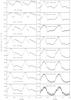 |
Fig. 1 Pulse profiles of 4U 0115 + 63 during observation (a) in different energy ranges. Data were collected with the MECS (2–8.5 keV), the HPGSPC (8.5–24 keV) and the PDS (24–90 keV). The phase-energy matrices of the three instruments were arbitrarily shifted by a few energy bins (maximum 3) to take their timing systematics into account and achieve an optimal alignment in their common energy ranges (8–11 keV for the MECS and HPGSPC, 20–25 keV for the HPGSPC and the PDS ). |
To extract the energy dependent pulse profiles and the phase resolved spectra, we binned the events recorded in each energy channel of each instruments in 100 (SAX) or 128 (RXTE) phase bins to form the “phase-energy matrices”. These matrices were then rebinned to achieve a sufficient S/N in each energy bin3 (at least 180 for BeppoSAX, and 60 for RXTE ). The exposure time of each phase bin was computed using the GTI of the corresponding observation and the reference time to fold the light curves was chosen so that the maximum of the high-energy pulse profiles in different observations remains at phase ~0.3.
3.2. Determination of phase lags
For all the observation in Table 1, we extracted a pulse profile in each of the energy bins of the phase-energy matrices (see Sect. 3.1). The pulse profiles showed a remarkable dependence on the energy (especially below ~5 keV), but did not change dramatically between the different observations. As an example, we show in Fig. 1 the pulse profiles extracted for the observation (a). Above ~5 keV, a prominent structure appears at phase ~0.3 (the “main peak”) and remains virtually stable at all the higher energies. The predominance of this structure is also confirmed by the analysis carried out in the left hand panel of Fig. 3. Here we represent with red (blue) colors the phases of all the pulse profiles extracted from the observations in Table 1 where the source count rate was higher (lower).
The relatively broad red spot, corresponding to the mean peak, seems to move in phase with the energy, thus showing a “phase-lag” in the pulse profiles. We note that this behavior is present in all observations. To investigate the origin of these phase lags in more detail, we extracted a reference pulse profile in the 8–10.5 keV energy range for each observation (see Fig. 2) and then computed the cross correlation between this reference profile and the pulse profiles extracted in different energy bands. We limit this analysis to the phases corresponding to the main peak (see Fig. 2) and use the discrete cross correlation function: 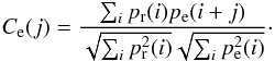 (1)Here, Ce(j) is the linear correlation coefficient calculated at the energy bin e and phase bin j. The indices of the phase bin for each pulse profile are j and i, while pr and pe are the reference and energy dependent pulse profiles, from which we subtracted their average values. The maximum value (and relative phase) of the correlation parameter for each energy bin, Ce,max, was estimated as a function of the phase by performing parabolic fits. Hereafter, we use normalized phase units, in which the phase is a real number in the range (0,1).
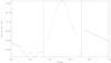 |
Fig. 2 Reference pulse profile of 4U 0115 + 63 extracted from observation (b). Data are from the PCA (energy range 8-10.5 keV). The pulse profile has been linearly scaled to have zero average and unitary standard deviation. The two vertical solid lines enclose the phase interval used for the correlation analysis: 0.33–0.72 (the phase is shifted with respect to Fig. 3 for clarity’s sake). |
A value of Ce,max ≪ 1 indicates that the pulse profiles pe extracted in the energy bin e are not strongly correlated with the reference pulse profile pr, so their shapes differ significantly. A value of Ce,max ~ 1 indicates that one profile can be obtained from the other using a linear function4 and intermediate values indicate a moderately different shape. The results of this analysis are shown in the right hand panel of Fig. 3 in a color representation and they provide a clear confirmation of significant phase lags in the energy-dependent pulse profiles.
A more quantitative representation of the measured phase lags is provided in Fig. 4. Here, we report the phase lags of the main peak for each observation with respect to the reference pulse, together with the corresponding uncertainties and the maximum correlation coefficient. To determine the phase lags and the associated uncertainties in the most appropriate way, we simulated 100 “phase-energy” matrices in which the number of events in each phase and energy bin was randomly selected from a Poisson distribution with an average value equal to the measured number of counts. We then carried out a correlation analysis for each of the simulated matrices and recorded the estimated phase lags. The measurement reported for each observation and energy bin in Fig. 4 was thus determined as the average of the simulated values and the corresponding uncertainty taken as one standard deviation form this value. We verified a posteriori that the values measured from the real data are consistent with the value obtained from the average of the simulations within the reported uncertainties.
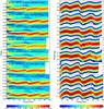 |
Fig. 3 Left panel: pulse profiles extracted from all the observations in Table 1 as a function of energy. Red (blue) colors indicate higher (lower) count rates at different pulse phases and energies. As discussed in Sect. 3.1, the higher intensity is around phase ~0.3, in correspondence with the “main peak”. The pulse profiles in this figure were all scaled to have in each energy bin a zero average value and a unitary standard deviation. Right panel: values of the correlation parameter Ce, as a function of phase lag with respect to the reference pulse profile and energy. Red (blue) colors indicate values of Ce close to unity ( ≪ 1). See text for details. |
The results reported in Fig. 4 show that the pattern of the phase lags vs. energy is very similar for all the observations. The main peak of the pulse is shifted toward lower phases at energies corresponding to the different absorption cyclotron features of 4U 0115 + 63. In correspondence of each of these shifts in phase, we also notice a deviation of the cross correlation coefficient from unity. This testifies that, at energies close to those of the different cyclotron features, the shape of the main peak is slightly different from that of the reference pulse profile. At the highest energies (40 keV), the marked decrease in the correlation coefficient is due to statistical noise. To correctly evidence the features visible that are in the pattern of the phase lags as a function of energy, we fit a model comprising several asymmetric Gaussian lines to these data5.
We note that the intrinsic energy resolutions of the different instruments (not accounted for in our phenomenological fit of the phase lags) affects the estimate of the centroid energies of the Gaussian empirical functions. From Fig. 4, it is clear that the third Gaussian is systematically detected with a centroid energy lower in the PDS than in the PCA data, because the former instrument is characterized by a lower energy resolution than the latter. The opposite effect is visible on the second Gaussian by comparing the PCA with the HPGSPC data, as the latter has a finer energy resolution than the former. Taking these systematic effects into account, we conclude that the phase lags measured from the different instruments and observations in Table 1 are in good agreement with each other, and no prominent variations of the phase lag pattern can be appreciated in the luminosity range of 4U 0115 + 63 spanned by the data.
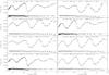 |
Fig. 4 Phase lags of the main peak in normalized phase units (points) and linear correlation coefficients (stars) as a function of energy. We considered here BeppoSAX data from the MECS (2–8.5 keV), the HPGSPC (8.5–25 keV), and the PDS (>25 keV). RXTE data are from the PCA (3–45 keV) and the HEXTE-B (>45 keV). The correlation function is computed on a phase interval of 0.4 phase units, centered on the maximum of the reference pulse profiles. The solid line represents the best-fit function to the phase lags (see text for the details). |
Finally, we checked that all the above results do not depend on the particular settings adopted in the method developed for the analysis described above. For this purpose, we performed a further analysis of the observation (b) by adopting different values of the range of both the phases used for the correlation analysis (Δφ) and the energy range chosen to extract the reference pulse profile (ΔE). All the results of this analysis are reported in Fig. 5. We note that the adoption of a smaller Δφ resulted in a significant decrease in the reliability of our analysis, as a large part of the peak falls outside the sampled window (also indicated by the lower value of the cross-correlation coefficient). Choosing a larger Δφ would instead lead to a loss of coherence in the cross-correlation due to the complex energy dependency of the pulse profiles outside the main peak. Changing the value of ΔE resulted, as expected, only in a systematic offset of the phase shifts. We thus concluded that the general trend of the phase shifts is not affected by the particular set of parameters used for the analysis.
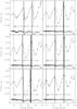 |
Fig. 5 Phase shifts measured from the observation (b) by using a different range of phases than adopted for the analysis in Fig. 4 to compute the shifts (Δφ) and a different energy range of the reference pulse profile (ΔE). Specific values of these parameters are indicated in different panels. The shaded intervals represent the centroid energy of the asymmetric Gaussians used to describe the lags with the 1σ uncertainty. The solid line is the best-fit function of the phase lags. |
3.3. Spectral analysis
In order to deeply investigate the relation between the phase lags and the energy of the cyclotron scattering features, we also performed a spectral analysis of the source.
We first extracted the phase-averaged spectra6 for each observation in Table 1 and performed a fit to these data with the phenomenological multicomponent model proposed for 4U 0115 + 63 by Ferrigno et al. (2009). For PCA, we added a 0.5% systematic error and fixed the absorption column at NH = 9 × 1021 cm-2, the best-fit value obtained in the BeppoSAX observations. This provided, in each case, an accurate measurements of the flux (and thus the luminosity) of the source (see Table 1). For each observation, we also report the centroid energy of the first three absorption lines in Fig. 6, together with the energy range at which the most negative phase lag occurs in the corresponding energy range. Although the most negative phase shifts occur slightly above the measured centroid energies for all lines, there is a clear indication of the link between timing and spectral features. In the following paragraphs, we clarify the origin of this apparent mismatch of energies.
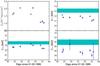 |
Fig. 6 Phase-averaged luminosity and centroid energy of the absorption lines. The horizontal cyan bands are the energy range of the most negative phase shift of the main peak measured from the BeppoSAX data. Uncertainties on fitted parameters are at 90% c.l. Upper left: X-ray luminosity (see Table 1). Upper right: centroid energy of the fundamental. Lower left: centroid energy of the first harmonic. Lower right: centroid energy of the second harmonic. |
A phase-resolved spectral analysis was carried out to study the variation in the properties of the cyclotron absorption lines at different phases (see e.g. Mihara et al. 2004). Following the discussion in Sect. 3.1, only the range of phases including the main peak was considered. We extracted source spectra in 64 and 50 phase bins for the PCA and the HPGSPC, respectively. We restricted the energy range for the phase-resolved analysis to the 10–35 keV interval and adopted in the fit a simplified spectral model comprising a power-law modified by a high-energy cut-off and three Gaussian absorption lines (gabs in XSPEC ). This permitted us to clearly identify the centroid energy of the fundamental and of the first harmonic in most spectra. We did check a posteriori that the simplified spectral model did not change our results significantly with respect to those already reported, e.g., by Ferrigno et al. (2009).
In Fig. 7, we show the values of the centroid, amplitude (σ), and optical depth (τ) of the fundamental vs. the pulse phase, while in Fig. 8, we show the corresponding results for the first harmonic for the three BeppoSAX observations. The pulse profiles in the relative energy ranges are also shown. For the second harmonic, we verified that the poorer S/N prevents such detailed analysis, by also using the PDS data to cover the range above 34 keV. The parameters of the lines could not be well constrained at different phases from those of the main peak, as in these cases the lines appeared absent or shallower and less pronounced. Despite the slightly different shape of the pulse profiles and the variation in the luminosity of the source (see Table 1), the three observations gave fairly similar results for the line parameters. This confirmed that the scattering region is located at roughly the same height above the NS in this luminosity range. In the upper right hand panel of these figures, we use a horizontal band to indicate the energy range in which the largest negative shift in phase of the pulse profiles in the BeppoSAX observations was measured. In both cases, the centroid energies correspond to the energy of the most negative phase shift in some phase interval. For the fundamental, such a phase range corresponds to the highest optical depth of the line, but to an intermediate value for the first harmonic. We notice that the phase resolved spectroscopy proves how the phase-averaged spectral results are a non-trivial average of phase variability and cannot be directly compared to our results for phase lags. For all the lines, the centroid energy estimated from the average spectra is lower than the energy of the corresponding phase lags, but the results of the phase-resolved spectroscopy clearly indicate that the energy dependency of the shift in phase of the pulse profiles is related to the cyclotron-scattering process. Similar results were obtained by performing a phase-resolved analysis of the RXTE data over a slightly wider range of luminosity.
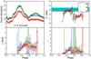 |
Fig. 7 Phase-resolved study of the fundamental absorption line for the BeppoSAX observations. Blue points correspond to observation (a), green circles to observation (d), and red diamonds to observation (f). Upper left: pulse profiles extracted in the energy range 11.2–13.2 keV (shifted in phase to be aligned). Upper right: centroid energy of the first cyclotron harmonic. The horizontal cyan band is the energy range of the most negative phase shift of the main peak measured from the SAX data. Lower left: amplitude of the line. Lower right: optical depth of the line. |
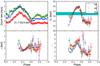 |
Fig. 8 Phase-resolved study of the first harmonic for the BeppoSAX observations. Blue points correspond to observation (a), green circles to observation (d), and red diamonds to observation (f). Uncertainties on fitted parameters are at 90% c.l. Upper left: pulse profiles extracted by using data from the HPGSPC in the energy range 21.7–23.5 keV. Upper right: centroid energy of the first cyclotron harmonics. The horizontal cyan band is the energy range of the most negative phase shift of the main peak measured from the BeppoSAX data. Lower left: amplitude of the line. Lower right: optical depth of the line. |
It is particularly interesting to note that in all cases the cyclotron lines get narrower and deeper in the descending edge of the pulse (i.e., the values of σ and τ are respectively lower and higher in these phases). We discuss this observational property of the line at the end of Sect. 4.
4. A model for the emission from an accretion column
In this section, we describe the model we developed to interpret the energy-dependent phase shifts of the pulse profiles from 4U 0115 + 63 and the properties of its cyclotron emission lines (see Sects. 3.2 and 3.3) in terms of an energy-dependent beamed emission emerging from two accretion columns on the NS. The model has a two-step structure: in the first part, we compute the flux emerging from the column as a function of its inclination angle with the line of sight (the “asymptotic beam pattern”). In the second part, we exploit the geometric parameters of 4U 0115 + 63 derived by Sasaki et al. (2011) using the pulse decomposition method to model the observed pulse profiles.
4.1. Asymptotic beam pattern of an accretion column
We considered in the model a spherical NS, with radius RNS and mass MNS. Based on the conclusion of Sasaki et al. (2011), we exclude the “hollow cone” geometry and then assume that the accretion column is homogeneously filled by the accreting material and characterized by a conical shape. The latter is a good approximation in case the accretion flow is confined by a dipolar magnetic field (Leahy 2003). Finally, we assume that the radiation is emitted from the lateral surface of the column, as expected for the X-ray luminosity of 4U 0115 + 63 in the observations analyzed here (LX ≃ 1038 erg s-1 > 4 × 1037 erg s-1Basko & Sunyaev 1976). As the emission from the accretion column is relatively close (at most a few km) to the NS surface, we also take the most relevant relativistic effects into account. We include in our model the relativistic beaming, the gravitational redshift and the gravitational lensing effect (also known as solid angle amplification), according to the method described by Leahy (2003). However, for the light bending, we use the approximate geodesic equation proposed by Beloborodov (2002)7. The mathematical details of the models are reported in Appendix A. The model parameters are thus the NS mass and radius, the semi-aperture of the accretion column, α0, the column height with respect to the NS surface, and the emissivity of the surface element of the column in its rest frame, I0,ν(r,φ0,α,φ1) (i.e., the intrinsic beam pattern). Here, ν is the radiation frequency, r the height at which the photon is emitted, φ0 its azimuth around the column axis, α the angle between the local radial direction and the photon trajectory, and φ1 is the corresponding azimuth (see Fig. A.1).
Deriving I0,ν(r,φ0,α,φ1) on a physical basis would require a detailed treatment of all the relevant photon-scattering processes in the accretion column, which is beyond the scope of the present paper. Instead, we consider a phenomenological model of I0,ν(r,φ0,α,φ1) depending just on the angle α. The dependency on φ1 can be neglected as the cyclotron scattering in the geometry considered here is almost independent from this angle, because the magnetic field lines are nearly perpendicular to the NS surface at the polar caps. We also assume that the intensity of the radiation emitted from the column does not depend on the radius r and the angle φ0. Including the dependence on φ0 could be relevant for tracing the coupling between the accretion disk with the magnetosphere. The dependency on r would account for the vertical density and velocity profiles in the accretion column (see also Leahy 2004a,b). We have verified that introducing a dependency of the emerging beam intensity on r does not have significant implications for the problem of modeling the observed phase shifts.
Our model of the radiation beaming comprises two emission components: one directed downwards and one upwards. Such beaming, at the end of our calculations, qualitatively reproduces the asymptotic beam patterns obtained by Sasaki et al. (2011) with the decomposition method (see Eq. (A.9)). The actual beaming is determined by the non-trivial interplay of special relativistic transformations due to the bulk motion of the emitting flow and anisotropic scattering. To estimate the magnitude of the special relativistic effects, we adopt the column model of Becker (1998) for two values of their parameter ϵc (0.5 and 1) defined in their Eq. (4.1). At the top of a 2 km column, the radiation advected downwards is two to three times more intense than the radiation escaping upwards for an isotropic field in the matter rest frame. The escaped radiation becomes nearly isotropic at the bottom of the column, where the flow settles. According to this model, most of the radiation is emitted in the lower part of the column, below the radiative shock, which is predicted to reside at a few hundred meters above the NS surface. Weighting the downward and upward emission with their emissivity does not affect our main assumption, as we find that the total downward radiation is 40–70% more intense than the upward one.
The bulk motion of the emitting plasma is not the only driver of the radiation beaming, because the scattering cross section are highly asymmetric in the strong magnetic field of HMXBs. Several studies have predicted a certain degree of anisotropy (see Kraus 2001, and references therein) for the radiation emitted far from the cyclotron resonances. More recently, Schönherr et al. (2007) have carried out MonteCarlo simulations and showed that the degree of anisotropy of the radiation in the energy range affected by the lines also depends on the optical depth of the plasma and does not exceed several percent (see their Fig. 7). No detailed studies have been carried out, to our knowledge, on the angular beaming of the radiation at energy close to the ones of the cyclotron scattering features, with the resolution required by the modern instruments. For this reason, our qualitative description of the radiation beam through the introduction of upwards and downwards components was mainly inspired by the study of the radiation spectral properties as a function of the viewing angle (see Schönherr et al. 2007, and references therein). For the results of the existing modeling8, we notice that the absorption line is deeper in the direction perpendicular to the magnetic field, thus resulting in an effective suppression of photon number in that direction. These photons are scattered primarly along the direction of the magnetic field, where the cross section is suppressed, and would presumably lead to an enhancement of the beamed radiation along the column axis. As the Doppler boosting is not extremely severe in the velocity field of the infalling plasma, we conclude that a considerable fraction of the photons will be able to escape in the vertical direction and originate to an upward directed component.
To summarize, we associate the downward component with the radiation advected by the plasma flow (as already proposed, see e.g., Kraus 2001) and the upward component, introduced here for the first time, with the (cyclotron) scattered radiation. The latter component should be prominent close to the NS surface, where the flow is characterized by a reduced bulk motion, but gives rise to a non-negligible contribution also along the column extension, owing to the relatively moderate Doppler boosting. We model the first component with a Gaussian centered on α = 150° and characterized by a width of 45° (normalization set arbitrarily to 100), and the second component with a Gaussian centered on the local zenith and characterized by a width of 45° and a variable normalization. Even though we use this heuristic approach, our model is able to qualitatively account for the most relevant properties of the intrinsic beam pattern emerging from the accretion column of 4U 0115 + 63.
Once I0,ν(α) is given, the asymptotic beam pattern can be computed as a function of the angle between the axis of the column and the line of sight to the observer (ψobs, see Appendix A for the details). In Fig. 9, we show the intrinsic beam patterns in the left hand panels, I0,ν(α), for different values of the normalization of the upward component. The corresponding asymptotic beam patterns are reported in the central panels. These were computed by assuming an accretion column of semi-aperture 4°, extended for 2 km above the surface of a canonical NS with mass 1.4 M⊙ and radius 10 km (column height from Nakajima et al. 2006). We notice that the shape of the beam is not very sensitive to the different parameters adopted for the column and the NS, provided that the upper part of the accretion column remains visible at large viewing angles ( ).
).
4.2. Simulated pulse profiles
Assuming the above asymptotic beam patterns, we computed the pulse profiles of 4U 0115 + 63 by using the geometrical parameters of the system described in Figs. 2 and 3 of Kraus et al. (1995, all measured with respect to the rotation axis of the NS). These are the direction of the line of sight to the source (Θ0), the colatitude of the two magnetic poles (Θ1, Θ2), and their difference in longitude (Δ). For the accretion column located on the i-magnetic pole, we can write the following relation between these angles: ![Mathematical equation: \begin{eqnarray} \lefteqn{\cos \psi_\mathrm{obs} = \cos \Theta_0 \cos \Theta_\mathrm{i} } \nonumber \\ & +\sin \Theta_0 \sin \Theta_i \cos \left[ \Omega (t-t_\mathrm{ref}) -(i-1)(\pi - \Delta ) \right], \label{eq:psi_obs} \end{eqnarray}](/articles/aa/full_html/2011/08/aa16826-11/aa16826-11-eq82.png) (2)where i = (1,2), and Ω = 2π/Pspin is the pulsar angular velocity measured at a reference time t = tref9. We assume in the following Θ0 = 60°, Θ1 = 148°, Θ2 = 74°, and Δ = 68° (Sasaki et al. 2011). As an example, we show the pulse profiles computed in the right hand panels of Fig. 9 by using the above geometrical parameters and the beam patterns reported in the central panels of the same figure. We did not consider other geometrical configurations, because we constructed the intrinsic beam pattern to reproduce the asymptotic beam pattern obtained for Θ0 = 60°. However, we verified that phase lags can be modeled also for other allowed configurations by adopting a different intrinsic beaming.
(2)where i = (1,2), and Ω = 2π/Pspin is the pulsar angular velocity measured at a reference time t = tref9. We assume in the following Θ0 = 60°, Θ1 = 148°, Θ2 = 74°, and Δ = 68° (Sasaki et al. 2011). As an example, we show the pulse profiles computed in the right hand panels of Fig. 9 by using the above geometrical parameters and the beam patterns reported in the central panels of the same figure. We did not consider other geometrical configurations, because we constructed the intrinsic beam pattern to reproduce the asymptotic beam pattern obtained for Θ0 = 60°. However, we verified that phase lags can be modeled also for other allowed configurations by adopting a different intrinsic beaming.
By comparing Figs. 1 and 9, we note that the model developed above can reproduce the shape of the pulse profiles of 4U 0115 + 63 relatively well at energies higher than the fundamental cyclotron scattering feature. In our model, the bump in the profile that follows the main peak is due to the emission from the accretion column closer to the observer’s line of sight. However, we note that the double-peak structure of the upward emission (represented by the dot-dashed line at phase 0.9–1.2 in Fig. 9), which results from the model, does not seem to be present in the observed pulse profiles. The suppression of the flux between these two peaks (at phase ~ 1.1) is unavoidable in the model, because it comes from the decreased flux of the asymptotic beam pattern at angles ψobs ≲ 30° produced by the self-obscuration of the column. The double peak could be avoided if the upward beam were emitted slightly outside the column (e.g., in a scattering halo near or on the NS surface), or if part of the radiation also escapes along the accretion column axis in a pencil beam. Our simplified model could not reproduce this kind of emission, as this would have required either a termination of the column at some height with emission from its top or the introduction of an emitting region around the column. However, we note that our calculation was not aimed at reproducing the exact shape of pulse profile, but rather at finding a plausible explanation for the phase lags observed in correspondence of the cyclotron lines, an effect which has never been reported before.
Indeed, the phase lags measured from the data are also reproduced relatively well in the model (see Fig. 9). According to our calculations, the displacement of the main peak in phase is due to the distortion of its shape at energies close to those of the cyclotron absorption lines, where the contribution of the upward Gaussian component to the intrinsic beam is enhanced. In our model, the larger estimated shift in phase is − 0.05 (measured in phase units, for N2 = 75–100), and the corresponding value of the cross-correlation coefficient is 0.85. The analysis was limited here to the phases 0.0–0.5 that correspond to the mean peak of the pulse profiles, see right panels of Fig. 9. This is in fairly good agreement with the results found from the data. We also note that the location of the main pulse peak moves to lower phases at low energy (E ≲ 5 keV), where a scattering halo on the NS surface dominates. This is a further indication that the scattered radiation is responsible for the observed phase shifts.
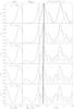 |
Fig. 9 Left panels: intrinsic beam patterns (arbitrary units) emerging from the lateral walls of the NS accretion column as a function of the angle α with respect to the local radial direction. The function is the sum of two Gaussians as described in Eq. (A.9). The value of the normalization of the upward Gaussian is indicated in each plot (N2). Central panels: asymptotic beam patterns (arbitrary units normalized to the values at 170 degrees) as a function of the angle ψobs between the axis of the accretion column and the line of sight to the observer. The beams are computed by assuming an accretion column with a semi-aperture of 4 degrees, and extended for 2 km above the surface of a neutron star with a mass of 1.4 M⊙ and a radius of 10 km. Right panels: synthetic pulse profiles computed for the geometry in 4U 0115 + 63 described in Sect. 4. The solid line corresponds to the total flux divided by two times its averaged value for plotting purposes. The dashed line represents the contribution from the farther pole from the line of sight to the observer, while the dot-dashed line indicates the contribution from the other pole. The gray vertical band corresponds to the location in phase of the pulse maximum. A leftward shift in phase is emerging while increasing the value of N2. |
Finally, we show that our model is compatible with the phase-resolved spectral properties of the absorption lines carried out in Sect. 3.3. In Fig. 10 (upper panel), we report the viewing angles (ψobs,i) of the two accretion columns onto the NS with respect to the line of sight as a function of the phase. We also plot the average viewing angle (solid line) calculated for the combined radiation of the two columns (weighted for their relative contribution estimated by using the beam pattern in our model), which results in a relatively large angle (~120−150°) on the descending portion of the main peak (phases ~ 0.3–0.6), and significantly lower values at other phases. To understand the meaning of these considerations, in the bottom panel of Fig. 10, we plot the relation between the angles α and ψ, which are calculated from the relativistic ray-tracing of the model (see also Fig. A.1). The former angle represents a good approximation of the relative direction between the radiation emerging from the column and the local magnetic field, while ψ is the trajectory deflection angle (see Fig. A.1), which differs from the column viewing angle (ψobs) by at most a few degrees. We note that ψ ~ 120−150° corresponds to α ~ 80−100°; therefore at the phases of the right flank of the main peak, the emerging radiation is emitted in a direction nearly perpendicular to the local magnetic field. At these inclinations, the resonant scattering features are expected to be deeper and narrower (see Schönherr et al. 2007, and references therein), in agreement with the results found from the phase-resolved spectral analysis carried out in Sect. 3.3.
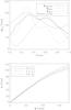 |
Fig. 10 Upper panel: inclination angles of the columns with respect to the line of sight to the observer obtained by assuming an intrinsic beam pattern with N2 = 25. The dashed line represents the column that is farther away from the observer; the dot-dashed line, the other. The solid line is the average inclination angle of the two columns weighted for their relative flux measured at the location of the observer. The dotted line is the synthetic pulse profile, scaled to fit into the plot. Lower panel: relation between the angles ψ and α of Fig. A.1 for different locations from the center of the NS in units of the gravitational radius. The three locations correspond to the base of the accretion column, its midpoint, and the top of the column, respectively (calculated according to the geometry of the system defined in Sect. 4). |
5. Discussion and conclusion
In this paper, we analyzed archival BeppoSAX and RXTE observations of 4U 0115 + 63 performed during the giant outburst of the source, which occurred in 1999. We investigated in particular the shape of the pulse profiles of the source at energies close to those of the cyclotron absorption features (~12, 24, 36, and 48 keV). At these energies, we measured a peculiar phase shift of the pulse profiles for the first time by using a cross-correlation method.
To interpret these findings, we created a geometrical model for the emission from an accretion column of a neutron star that considers the most relevant relativistic effects. The intrinsic beam pattern was calculated by assuming a parameterization for the emission with both a downward and an upward beam, which mimics the presence of the radiation advected in the column by the in-falling accreting material and the effect of resonant scattering. This model permits the reconstruction of the asymptotic beam patterns from 4U 0115 + 63 as perceived by a distant observer and thus the calculation of the simulated pulse profiles from the source by adopting the geometrical parameters determined by Sasaki et al. (2011).
Our method reproduced the general shape of the observed pulse profiles from 4U 0115 + 63 relatively well and the properties of their energy-dependent phase shifts described in Sect. 3.2. According to our interpretation, these phase shifts can stem from an energy-dependent beaming of the radiation, which we modeled as a variable contribution of the upward directed beam, whose origin can be ascribed to the resonant nature of the scattering cross-section in a strong magnetic field. The modeled pulse profiles get distorted at the energies corresponding to the CRSFs, creating a negative shift in phase that is in fairly good agreement with what is inferred from the observations. With the adopted system geometry, we were also able to naturally explain the phase-dependent measured properties of the absorption lines.
Although we adopted a phenomenological description of the radiation emerging from the accretion column of an HMXB, our calculations revealed the key role of an energy-dependent beaming for the pulse profile formation mechanism. Based on this idea, we were able to point out a plausible explanation for the energy-dependent phase shifts that we discovered. A more complex approach, which will solve the radiation transport problem using the actual cross sections and a realistic column velocity profile, will provide a self-consistent model of the spectral and timing characteristics of the XRB X-ray emission.
Significant changes of the pulse profiles with the energy, especially close to the resonances of the cyclotron scattering cross-section, have been reported so far in a number of different XRBPs (e.g., V 0332 + 53 Tsygankov et al. 2006). Applying the analysis method developed here to these other sources is ongoing and will be published elsewhere.
Online material
Appendix A: Calculation of the observed flux from an accretion column
We present a relativistic ray-tracing computations of the beam pattern emitted from the accretion column surface of a slowly rotating neutron star to model the phase lags observed in the X-ray pulse profiles of 4U 0115 + 63. We consider the geometrical properties of the column and the relativistic effects, i.e., light bending and the lensing effect in a Schwarzschild metric. Since the NS is slowly rotating, the relativistic travel time delay and the Doppler boosting have not been taken into account. The observer is located at positive infinity on the z-axis in the non-rotating observer frame with polar coordinates (r,θ,φ). The accretion column reference frame has the polar coordinates (r′,θ′,φ′) with the z′-axis coincident with the accretion column axis. See Fig. A.1 for the geometry of the systems. The deflection angle of a photon emitted from the accretion column surface is ψ, while α indicates the angle between the local radial direction and the photon direction at the emission point.
A.1. Light bending
The geodetic equation for an emitting position of a photon depends on the impact parameter, b (Misner et al. 1973), which is defined as 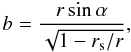 (A.1)where r is the radial coordinate of the emitting surface element, and rs = 2GM/c2 is defined as the Schwarzschild radius.
The relation between α and the photon deflection angle, ψ, i.e., the light bending, can be directly obtained using the approximated null geodetic equation, strictly valid for α < π/2 (see Beloborodov 2002, for more details): 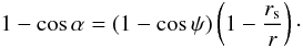 (A.2)For each column surface element at a given column orientation, ψobs, (see Eq. (2)), we determine the angle, α, and ,therefore, ψ, at which the emitted radiation reaches the observer (the only trajectories considered for the pulse profile modeling10).
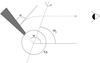 |
Fig. A.1 The geometry of the systems (not in scale). The dashed line shows a photon trajectory from the accretion column surface to the observer located at infinity, the dot-dashed line is the rotational axis of the NS. |
For photons emitted towards the NS surface (α > π/2), the allowed α values can be estimated by imposing that the trajectory not be swallowed by the relativistic photosphere of the compact object. This translates into the relation π/2 < α < αmax, where ![Mathematical equation: \appendix \setcounter{section}{1} \begin{equation} \alpha_\mathrm{max}=\pi - \sin^{-1} \left( \frac{3}{2} \sqrt{3 \left[1- \frac{r_\mathrm{s}}{r} \right]} \frac{r_\mathrm{s}}{r} \right), \end{equation}](/articles/aa/full_html/2011/08/aa16826-11/aa16826-11-eq116.png) (A.3)and r is the radial coordinate at which the photon is emitted from the column (e.g., point B in Fig. A.2). These trajectories have a “turning point” and thus possess a periastron; it is then convenient to express all relevant quantities in terms of the periastron distance, p. For αmax > αB > π/2, we first compute the impact parameter using Eq. (A.1), and then estimate the value p of the periastron by taking the largest real solution of the equation p3 − b2p + b2rs = 0. This equation is obtained by setting α = π/2 and r = p in Eq. (A.1), as αp = π/2 at the periastron. Using Eq. (A.2), we find ψp = cos-1(1 − 1/[1 − rs/p]) . The photon trajectory again reaches the radial coordinate r at point A (see Fig. A.2), where the angle formed by the photon with the local radial direction is αA = π − αB. The angle ψA can now be computed from Eq. (A.2). Finally, from simple symmetry considerations,
(A.3)and r is the radial coordinate at which the photon is emitted from the column (e.g., point B in Fig. A.2). These trajectories have a “turning point” and thus possess a periastron; it is then convenient to express all relevant quantities in terms of the periastron distance, p. For αmax > αB > π/2, we first compute the impact parameter using Eq. (A.1), and then estimate the value p of the periastron by taking the largest real solution of the equation p3 − b2p + b2rs = 0. This equation is obtained by setting α = π/2 and r = p in Eq. (A.1), as αp = π/2 at the periastron. Using Eq. (A.2), we find ψp = cos-1(1 − 1/[1 − rs/p]) . The photon trajectory again reaches the radial coordinate r at point A (see Fig. A.2), where the angle formed by the photon with the local radial direction is αA = π − αB. The angle ψA can now be computed from Eq. (A.2). Finally, from simple symmetry considerations, 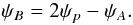 (A.4)This characterizes the considered trajectory fully, since the impact parameter for ψA has the same value as for the deflection angle at the emission point, ψB.
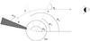 |
Fig. A.2 Schematic representation of a photon trajectory (dashed line) from the accretion column surface to the distant observer for trajectories with a turning point (not in scale). The emission point is B and the angle to be computed is ψB. A is the point at which the trajectory reaches for the second time the radial coordinate at which it originated. p indicates the location of the trajectory’s periastron. |
For each photon-emitting point we can now follow the photon trajectory to verify if it is absorbed by the NS or accretion column surface. For α < π/2, the trajectory can be directly computed using the following equation (Beloborodov 2002): ![Mathematical equation: \appendix \setcounter{section}{1} \begin{equation} \widehat{r}(\widehat{\psi}) = \left[ \frac { r_\mathrm{s}^2 ( 1- \cos \widehat{\psi})^2}{4 (1+\cos \widehat{\psi} )^2} + \frac{b^2}{\sin^2\widehat{\psi}}\right]^2 - \frac{r_\mathrm{s}^2 (1-\cos\widehat{\psi})}{2(1-\cos\widehat{\psi})}\,, \end{equation}](/articles/aa/full_html/2011/08/aa16826-11/aa16826-11-eq134.png) (A.5)where
(A.5)where  values are in the range (0,ψ).
For α > π/2, we use Eq. (A.1) to link  to
to  along the trajectory (the impact parameter b is constant in each geodesic). The corresponding value of is found with the method outlined above. The trajectories that hit the NS or intersect one of the optically thick accretion columns are excluded from the computation of the source flux measured at the observer’s location.
A.2. Lensing and red shift
We now compute the flux emitted by the column and measured by a distant observer. The flux emitted by a surface element from the accretion column, when it reaches the observed plane normal to the direction of the line of sight, is given by dFν = IνdΩ, where the solid angle can be expressed in terms of the impact parameter (Misner et al. 1973): 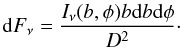 (A.6)Here, φ is the azimuthal angle around the line of sight of the plane containing the trajectory of the photon, and Iν(b,φ) is the differential intensity of the radiation emitted by the surface element when it reaches the observed plane at a distance D.
The impact factor b depends on r and α, but not on φ. The angle α can be expressed as a function of r and ψ, as shown in the previous section. We further note that the differential in Eq. (A.6) can be expressed as db = (db/dr)ψdr + (db/dψ)rdψ, and is computed along a line on a geometrical cone at constant φ, which is by definition a radial line. Therefore we can simplify the differential and write db = (db/dr)ψdr, since ψ is constant along a radial line.
Up to this point we expressed the equations in the observer’s reference frame defined above. To integrate the emission on the column surface, we transform the integration variables to the column’s frame to use quantities directly related to the accretion column. The Jacobian of the coordinate transformation involves only the variables r (constant) and φ, and is: |dφ/dφ′|; therefore, Eq. (A.6) can be written as 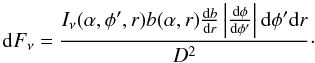 (A.7)We still need to express Iν in the system of reference of the column to account for the gravitational red-shift. Since I/ν3 is a Lorentz invariant, we can write
 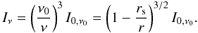 (A.8)As already described in Sect. 4, knowing the exact functional shape of I0,ν0(r,α) would require a detailed treatment of the cyclotron scattering process in a strong magnetic field (B ~ 1012 G) and of the relativistic beaming caused by the bulk motion of the plasma in the accretion column above the surface of the NS. This is outside the scope of the present paper. Instead, we aim at reproducing the beam pattern in the energy range of interest (>10 keV) found by using the pulse decomposition method described in Sasaki et al. (2011). For this purpose, we use a combination of two Gaussians, one pointed downwards and one upwards characterized by different amplitudes:
 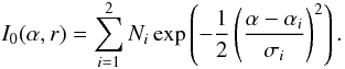 (A.9)\newpageIn the equation above, α1 = 150°, α2 = 0°, σ1 = 45°, σ2 = 45°, N1 = 100, and N2 assumed values from 0 to 100 to mimic a variable contribution from the cyclotron scattered radiation (See also Sect. 4).
The total flux emitted by the column is finally estimated from Eqs. (A.7)–(A.9) performing a Monte-Carlo integration with φ′ ∈ (0,2π), and r ∈ (rNS,rmax). The maximum height for the accretion column is equal to rmax − rNS. We did not include in the total flux the contribution of the photons that hit the NS surface and/or are absorbed by the column.
To verify the consistency of our results with similar calculations published before, we show in Fig. A.3 the beam patterns obtained from an isotropic emission on the lateral surface of an accretion column with the same configuration adopted in Fig. 3 of Riffert & Meszaros (1988). We found fairly good agreement between our results and those published by these authors. There is only a negligible discrepancy in the estimated fluxes of an accretion column extending up to 3.9 gravitational radii above the NS surface. Exact calculations predict that the critical height of a column for its total obscuration in the antipodal position should be 3.94rs. With the approximation used in our calculations, we obtained a value of 3.85rs. This discrepancy can only be relevant for a height of the column that is close to this critical value and for angles close to the antipodal position. Our approximation thus gives a satisfiable result for the accuracy required in the present work.
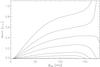 |
Fig. A.3 Column beam pattern seen by a distant observer and calculated for an isotropic emission in the case of a NS with a radius r = 3rS. The accretion column is assumed to have an half-aperture of 5 degrees, and an heights of (from bottom to top) 3.03, 3.15, 3.3, 3.6, 3.9, 4.2, and 4.6 rS. The angle ψ is measured from the line of sight to the axis of the column. |
In this paper, the “intrinsic beam pattern” is the intensity of radiation as a function of its orientation with respect to the infinitesimal surface element on the column surface, measured in the frame comoving with the column. The “asymptotic beam pattern” or “beam pattern” is an estimate of the flux integrated along the column surface as a function of the angle formed by the column axis with respect to the line of sight to the observer. It is measured at the location of the observer, and can be obtained from the intrinsic beam pattern after accounting for the general relativistic effects. Only the pulse profile can be measured directly from the observations.
The basic assumption is the equality of the beam patterns of the two accretion columns. Moreover, the decomposition is unique only if the angle between the rotation axis and the line of sight is known, otherwise this angle must be assumed.
We optimized these values for our analysis on a trial basis. The different values come from the different energy resolutions of the instruments.
The profiles in Eq. (1) have zero average but not unitary standard deviation, therefore in the ideal case of Ce,max = 1, they are related by a function that produces a phase shift and a rescale.
The empirical function used to fit the phase-lag energy dependency is ![Mathematical equation: \hbox{$f(e)=A+\sum_{i=1}^{4}N_i \exp \left[ -\left( e - E_i \right) ^2 / \sigma_{i,\lbrace d, u \rbrace }^2\right] $}](/articles/aa/full_html/2011/08/aa16826-11/aa16826-11-eq168.png) , where σi, { d,u } = σi,d for e ≤ Ei, σi, { d,u } = σi,u for e > Ei, and e is the energy. The fourth Gaussian is only poorly determined due to the low S/N of the data.
, where σi, { d,u } = σi,d for e ≤ Ei, σi, { d,u } = σi,u for e > Ei, and e is the energy. The fourth Gaussian is only poorly determined due to the low S/N of the data.
For the phase-averaged spectral analysis of the RXTE observations, we used the standard2 mode of the PCA data and both HEXTE units. For the spectral fitting, we used the XSPEC software (v.12.6.0u).
The range of validity of this approximation was extended as described in Appendix. A to account for the photons emitted above the NS surface in a downwards direction.
We concentrate our attention to the first harmonic, for which there is no photon spawning, which would add an unnecessary complication to our reasoning.
The spin period of accreting pulsars is not constant due to the torque exercised by the in-falling mass.
We neglect values of the angle ψ such that ψ > π. For these values multiple images of an emitting point could be formed. This is marginally relevant only for an accretion column located behind the NS, and thus not for 4U 0115 + 63 (see Sect. 4).
Acknowledgments
This research made use of data obtained through the High Energy Astrophysics Science Archive Research Center Online Service, provided by the NASA/Goddard Space Flight Center and the archive of BeppoSAX data available at the ASDC of ASI. C.F. thanks the research groups of IAA-Tübingen and Dr. Remeis-Sternwarte in Bamberg for developing and making available useful scripts to analyze RXTE data and A. Segreto for providing the software to perform phase resolved analysis of the BeppoSAX data. He also acknowledges illuminating discussions with J. Wilms and S. Paltani on the timing techniques, and the help of R. Doroshenko for the reduction of some BeppoSAX data. We thank ISSI for hosting and financing International group meetings on modeling and observations of cyclotron lines in High Mass X-ray binaries.
References
- Araya-Góchez, R. A., & Harding, A. K. 2000, ApJ, 544, 1067 [NASA ADS] [CrossRef] [Google Scholar]
- Basko, M. M., & Sunyaev, R. A. 1976, MNRAS, 175, 395 [NASA ADS] [CrossRef] [Google Scholar]
- Becker, P. A. 1998, ApJ, 498, 790 [NASA ADS] [CrossRef] [Google Scholar]
- Becker, P. A., & Wolff, M. T. 2007, ApJ, 654, 435 [NASA ADS] [CrossRef] [Google Scholar]
- Beloborodov, A. M. 2002, ApJ, 566, L85 [NASA ADS] [CrossRef] [Google Scholar]
- Blum, S., & Kraus, U. 2000, ApJ, 529, 968 [NASA ADS] [CrossRef] [Google Scholar]
- Boella, G., Butler, R. C., Perola, G. C., et al. 1997a, A&AS, 122, 299 [NASA ADS] [CrossRef] [EDP Sciences] [Google Scholar]
- Boella, G., Chiappetti, L., Conti, G., et al. 1997b, A&AS, 122, 327 [NASA ADS] [CrossRef] [EDP Sciences] [Google Scholar]
- Bradt, H. V., Rothschild, R. E., & Swank, J. H. 1993, A&AS, 97, 355 [NASA ADS] [Google Scholar]
- Caballero, I., Kraus, U., Santangelo, A., Sasaki, M., & Kretschmar, P. 2011, A&A, 526, A131 [NASA ADS] [CrossRef] [EDP Sciences] [Google Scholar]
- Cominsky, L., Clark, G. W., Li, F., Mayer, W., & Rappaport, S. 1978, Nature, 273, 367 [NASA ADS] [CrossRef] [Google Scholar]
- Davidson, K., & Ostriker, J. P. 1973, ApJ, 179, 585 [NASA ADS] [CrossRef] [Google Scholar]
- Ferrigno, C., Segreto, A., Santangelo, A., et al. 2007, A&A, 462, 995 [NASA ADS] [CrossRef] [EDP Sciences] [Google Scholar]
- Ferrigno, C., Becker, P. A., Segreto, A., Mineo, T., & Santangelo, A. 2009, A&A, 498, 825 [NASA ADS] [CrossRef] [EDP Sciences] [Google Scholar]
- Frank, J., King, A., & Raine, D. J. 2002, Accretion Power in Astrophysics (Cambridge University Press) [Google Scholar]
- Frontera, F., Costa, E., dal Fiume, D., et al. 1997, A&AS, 122, 357 [NASA ADS] [CrossRef] [EDP Sciences] [Google Scholar]
- Giacconi, R., Gursky, H., Kellogg, E., Schreier, E., & Tananbaum, H. 1971, ApJ, 167, L67 [NASA ADS] [CrossRef] [Google Scholar]
- Heindl, W. A., Coburn, W., Gruber, D. E., et al. 1999, ApJ, 521, L49 [NASA ADS] [CrossRef] [Google Scholar]
- Heindl, W. A., Rothschild, R. E., Coburn, W., et al. 2004, X-RAY TIMING 2003: Rossie and Beyond, AIP Conf. Proc., 714, 323 [Google Scholar]
- Isenberg, M., Lamb, D. Q., & Wang, J. C. L. 1998, ApJ, 505, 688 [NASA ADS] [CrossRef] [Google Scholar]
- Jahoda, K., Swank, J. H., Giles, A. B., et al. 1996, Proc. SPIE, 2808, 59 [NASA ADS] [CrossRef] [Google Scholar]
- Johns, M., Koski, A., Canizares, C., et al. 1978, IAU Circ., 3171 [Google Scholar]
- Klochkov, D., Santangelo, A., Staubert, R., & Ferrigno, C. 2008, A&A, 491, 833 [NASA ADS] [CrossRef] [EDP Sciences] [Google Scholar]
- Kraus, U. 2001, ApJ, 563, 289 [NASA ADS] [CrossRef] [Google Scholar]
- Kraus, U., Herold, H., Maile, T., Nollert, H.-P., & Rebetzky, A. 1989, A&A, 223, 246 [NASA ADS] [Google Scholar]
- Kraus, U., Nollert, H.-P., Ruder, H., & Riffert, H. 1995, ApJ, 450, 763 [NASA ADS] [CrossRef] [Google Scholar]
- Kraus, U., Blum, S., Schulte, J., Ruder, H., & Meszaros, P. 1996, ApJ, 467, 794 [NASA ADS] [CrossRef] [Google Scholar]
- Kraus, U., Zahn, C., Weth, C., & Ruder, H. 2003, ApJ, 590, 424 [NASA ADS] [CrossRef] [Google Scholar]
- Leahy, D. A. 1990, MNRAS, 242, 188 [NASA ADS] [Google Scholar]
- Leahy, D. A. 1991, MNRAS, 251, 203 [NASA ADS] [Google Scholar]
- Leahy, D. A. 2003, ApJ, 596, 1131 [NASA ADS] [CrossRef] [Google Scholar]
- Leahy, D. A. 2004a, MNRAS, 348, 932 [NASA ADS] [CrossRef] [Google Scholar]
- Leahy, D. A. 2004b, ApJ, 613, 517 [NASA ADS] [CrossRef] [Google Scholar]
- Leahy, D. A., & Li, L. 1995, MNRAS, 277, 1177 [NASA ADS] [Google Scholar]
- Manzo, G., Giarrusso, S., Santangelo, A., et al. 1997, A&AS, 122, 341 [NASA ADS] [CrossRef] [EDP Sciences] [Google Scholar]
- Meszaros, P., & Nagel, W. 1985a, ApJ, 298, 147 [NASA ADS] [CrossRef] [Google Scholar]
- Meszaros, P., & Nagel, W. 1985b, ApJ, 299, 138 [CrossRef] [Google Scholar]
- Meszaros, P., & Riffert, H. 1988, ApJ, 327, 712 [NASA ADS] [CrossRef] [Google Scholar]
- Mihara, T., Makishima, K., & Nagase, F. 2004, ApJ, 610, 390 [NASA ADS] [CrossRef] [Google Scholar]
- Misner, C. W., Thorne, K. S., & Wheeler, J. A. 1973 (San Francisco: W.H. Freeman and Co.) [Google Scholar]
- Nakajima, M., Mihara, T., Makishima, K., & Niko, H. 2006, ApJ, 646, 1125 [NASA ADS] [CrossRef] [Google Scholar]
- Negueruela, I., & Okazaki, A. T. 2001, A&A, 369, 108 [NASA ADS] [CrossRef] [EDP Sciences] [Google Scholar]
- Negueruela, I., Okazaki, A. T., Fabregat, J., et al. 2001, A&A, 369, 117 [NASA ADS] [CrossRef] [EDP Sciences] [Google Scholar]
- Pringle, J. E., & Rees, M. J. 1972, A&A, 21, 1 [NASA ADS] [Google Scholar]
- Rappaport, S., Clark, G. W., Cominsky, L., Li, F., & Joss, P. C. 1978, ApJ, 224, L1 [NASA ADS] [CrossRef] [Google Scholar]
- Riffert, H., & Meszaros, P. 1988, ApJ, 325, 207 [NASA ADS] [CrossRef] [Google Scholar]
- Riffert, H., Nollert, H.-P., Kraus, U., & Ruder, H. 1993, ApJ, 406, 185 [NASA ADS] [CrossRef] [Google Scholar]
- Rothschild, R. E., Blanco, P. R., Gruber, D. E., et al. 1998, ApJ, 496, 538 [NASA ADS] [CrossRef] [Google Scholar]
- Santangelo, A., Segreto, A., Giarrusso, S., et al. 1999, ApJ, 523, L85 [NASA ADS] [CrossRef] [Google Scholar]
- Sasaki, M., Klochkov, D., Kraus, U., Caballero, I., & Santangelo, A. 2010, A&A, 517, A8 [NASA ADS] [CrossRef] [EDP Sciences] [Google Scholar]
- Sasaki, M., Müller, D., Kraus, U., Ferrigno, C., & Santangelo, A. 2011, A&A, submitted [Google Scholar]
- Schönherr, G., Wilms, J., Kretschmar, P., et al. 2007, A&A, 472, 353 [NASA ADS] [CrossRef] [EDP Sciences] [Google Scholar]
- Tamura, K., Tsunemi, H., Kitamoto, S., Hayashida, K., & Nagase, F. 1992, ApJ, 389, 676 [NASA ADS] [CrossRef] [Google Scholar]
- Tananbaum, H., Gursky, H., Kellogg, E. M., et al. 1972, ApJ, 174, L143 [NASA ADS] [CrossRef] [Google Scholar]
- Tsygankov, S. S., Lutovinov, A. A., Churazov, E. M., & Sunyaev, R. A. 2006, MNRAS, 371, 19 [NASA ADS] [CrossRef] [Google Scholar]
- Tsygankov, S. S., Lutovinov, A. A., Churazov, E. M., & Sunyaev, R. A. 2007, Astronomy Letters, 33, 368 [NASA ADS] [CrossRef] [Google Scholar]
- Tsygankov, S. S., Lutovinov, A. A., & Serber, A. V. 2010, MNRAS, 401, 1628 [NASA ADS] [CrossRef] [Google Scholar]
- Wasserman, I., & Shapiro, S. L. 1983, ApJ, 265, 1036 [NASA ADS] [CrossRef] [Google Scholar]
- Wheaton, W. A., Doty, J. P., Primini, F. A., et al. 1979, Nature, 282, 240 [NASA ADS] [CrossRef] [Google Scholar]
- White, N. E., Swank, J. H., & Holt, S. S. 1983, ApJ, 270, 711 [NASA ADS] [CrossRef] [Google Scholar]
- Whitlock, L., Roussel-Dupre, D., & Priedhorsky, W. 1989, ApJ, 338, 381 [NASA ADS] [CrossRef] [Google Scholar]
All Tables
All Figures
|
Fig. 1 Pulse profiles of 4U 0115 + 63 during observation (a) in different energy ranges. Data were collected with the MECS (2–8.5 keV), the HPGSPC (8.5–24 keV) and the PDS (24–90 keV). The phase-energy matrices of the three instruments were arbitrarily shifted by a few energy bins (maximum 3) to take their timing systematics into account and achieve an optimal alignment in their common energy ranges (8–11 keV for the MECS and HPGSPC, 20–25 keV for the HPGSPC and the PDS ). |
| In the text | |
|
Fig. 2 Reference pulse profile of 4U 0115 + 63 extracted from observation (b). Data are from the PCA (energy range 8-10.5 keV). The pulse profile has been linearly scaled to have zero average and unitary standard deviation. The two vertical solid lines enclose the phase interval used for the correlation analysis: 0.33–0.72 (the phase is shifted with respect to Fig. 3 for clarity’s sake). |
| In the text | |
|
Fig. 3 Left panel: pulse profiles extracted from all the observations in Table 1 as a function of energy. Red (blue) colors indicate higher (lower) count rates at different pulse phases and energies. As discussed in Sect. 3.1, the higher intensity is around phase ~0.3, in correspondence with the “main peak”. The pulse profiles in this figure were all scaled to have in each energy bin a zero average value and a unitary standard deviation. Right panel: values of the correlation parameter Ce, as a function of phase lag with respect to the reference pulse profile and energy. Red (blue) colors indicate values of Ce close to unity ( ≪ 1). See text for details. |
| In the text | |
|
Fig. 4 Phase lags of the main peak in normalized phase units (points) and linear correlation coefficients (stars) as a function of energy. We considered here BeppoSAX data from the MECS (2–8.5 keV), the HPGSPC (8.5–25 keV), and the PDS (>25 keV). RXTE data are from the PCA (3–45 keV) and the HEXTE-B (>45 keV). The correlation function is computed on a phase interval of 0.4 phase units, centered on the maximum of the reference pulse profiles. The solid line represents the best-fit function to the phase lags (see text for the details). |
| In the text | |
|
Fig. 5 Phase shifts measured from the observation (b) by using a different range of phases than adopted for the analysis in Fig. 4 to compute the shifts (Δφ) and a different energy range of the reference pulse profile (ΔE). Specific values of these parameters are indicated in different panels. The shaded intervals represent the centroid energy of the asymmetric Gaussians used to describe the lags with the 1σ uncertainty. The solid line is the best-fit function of the phase lags. |
| In the text | |
|
Fig. 6 Phase-averaged luminosity and centroid energy of the absorption lines. The horizontal cyan bands are the energy range of the most negative phase shift of the main peak measured from the BeppoSAX data. Uncertainties on fitted parameters are at 90% c.l. Upper left: X-ray luminosity (see Table 1). Upper right: centroid energy of the fundamental. Lower left: centroid energy of the first harmonic. Lower right: centroid energy of the second harmonic. |
| In the text | |
|
Fig. 7 Phase-resolved study of the fundamental absorption line for the BeppoSAX observations. Blue points correspond to observation (a), green circles to observation (d), and red diamonds to observation (f). Upper left: pulse profiles extracted in the energy range 11.2–13.2 keV (shifted in phase to be aligned). Upper right: centroid energy of the first cyclotron harmonic. The horizontal cyan band is the energy range of the most negative phase shift of the main peak measured from the SAX data. Lower left: amplitude of the line. Lower right: optical depth of the line. |
| In the text | |
|
Fig. 8 Phase-resolved study of the first harmonic for the BeppoSAX observations. Blue points correspond to observation (a), green circles to observation (d), and red diamonds to observation (f). Uncertainties on fitted parameters are at 90% c.l. Upper left: pulse profiles extracted by using data from the HPGSPC in the energy range 21.7–23.5 keV. Upper right: centroid energy of the first cyclotron harmonics. The horizontal cyan band is the energy range of the most negative phase shift of the main peak measured from the BeppoSAX data. Lower left: amplitude of the line. Lower right: optical depth of the line. |
| In the text | |
|
Fig. 9 Left panels: intrinsic beam patterns (arbitrary units) emerging from the lateral walls of the NS accretion column as a function of the angle α with respect to the local radial direction. The function is the sum of two Gaussians as described in Eq. (A.9). The value of the normalization of the upward Gaussian is indicated in each plot (N2). Central panels: asymptotic beam patterns (arbitrary units normalized to the values at 170 degrees) as a function of the angle ψobs between the axis of the accretion column and the line of sight to the observer. The beams are computed by assuming an accretion column with a semi-aperture of 4 degrees, and extended for 2 km above the surface of a neutron star with a mass of 1.4 M⊙ and a radius of 10 km. Right panels: synthetic pulse profiles computed for the geometry in 4U 0115 + 63 described in Sect. 4. The solid line corresponds to the total flux divided by two times its averaged value for plotting purposes. The dashed line represents the contribution from the farther pole from the line of sight to the observer, while the dot-dashed line indicates the contribution from the other pole. The gray vertical band corresponds to the location in phase of the pulse maximum. A leftward shift in phase is emerging while increasing the value of N2. |
| In the text | |
|
Fig. 10 Upper panel: inclination angles of the columns with respect to the line of sight to the observer obtained by assuming an intrinsic beam pattern with N2 = 25. The dashed line represents the column that is farther away from the observer; the dot-dashed line, the other. The solid line is the average inclination angle of the two columns weighted for their relative flux measured at the location of the observer. The dotted line is the synthetic pulse profile, scaled to fit into the plot. Lower panel: relation between the angles ψ and α of Fig. A.1 for different locations from the center of the NS in units of the gravitational radius. The three locations correspond to the base of the accretion column, its midpoint, and the top of the column, respectively (calculated according to the geometry of the system defined in Sect. 4). |
| In the text | |
|
Fig. A.1 The geometry of the systems (not in scale). The dashed line shows a photon trajectory from the accretion column surface to the observer located at infinity, the dot-dashed line is the rotational axis of the NS. |
| In the text | |
|
Fig. A.2 Schematic representation of a photon trajectory (dashed line) from the accretion column surface to the distant observer for trajectories with a turning point (not in scale). The emission point is B and the angle to be computed is ψB. A is the point at which the trajectory reaches for the second time the radial coordinate at which it originated. p indicates the location of the trajectory’s periastron. |
| In the text | |
|
Fig. A.3 Column beam pattern seen by a distant observer and calculated for an isotropic emission in the case of a NS with a radius r = 3rS. The accretion column is assumed to have an half-aperture of 5 degrees, and an heights of (from bottom to top) 3.03, 3.15, 3.3, 3.6, 3.9, 4.2, and 4.6 rS. The angle ψ is measured from the line of sight to the axis of the column. |
| In the text | |
Current usage metrics show cumulative count of Article Views (full-text article views including HTML views, PDF and ePub downloads, according to the available data) and Abstracts Views on Vision4Press platform.
Data correspond to usage on the plateform after 2015. The current usage metrics is available 48-96 hours after online publication and is updated daily on week days.
Initial download of the metrics may take a while.