| Issue |
A&A
Volume 525, January 2011
|
|
|---|---|---|
| Article Number | A151 | |
| Number of page(s) | 15 | |
| Section | Interstellar and circumstellar matter | |
| DOI | https://doi.org/10.1051/0004-6361/201015049 | |
| Published online | 09 December 2010 | |
Rotating toroids in G10.62–0.38, G19.61–0.23, and G29.96–0.02⋆
1
INAF, Osservatorio Astrofisico di Arcetri, Largo E. Fermi 5, 50125
Firenze, Italy
e-mail: mbeltran@arcetri.astro.it
2
IRAM, 300 rue
de la Piscine, 38406
Saint Martin d’Hères,
France
Received: 26 May 2010
Accepted: 1 October 2010
Context. In recent years, we have detected clear evidence of rotation in more than 5 hot molecular cores (HMCs). Their identification is confirmed by the fact that the rotation axes are parallel to the axes of the associated bipolar outflows. We have now pursued our investigation by extending the sample to 3 known massive cores, G10.62–0.38, G19.61–0.23, and G29.96–0.02.
Aims. We wish to make a thorough study of the structure and kinematics of HMCs and corresponding molecular outflows to reveal possible velocity gradients indicative of the rotation of the cores.
Methods. We carried out PdBI observations at 2.7 and 1.4 mm of gas and dust with angular resolutions of ~2′′–3′′ and ~1′′–2′′, respectively. To trace both rotation and expansion, we simultaneously observed CH3CN, a typical HMC tracer, and 13CO, a typical outflow tracer.
Results. The CH3CN (12–11) observations reveal clear velocity gradients in the three HMCs oriented perpendicular to the direction of the bipolar outflows. For G19 and G29 the molecular outflows have been mapped in 13CO. The gradients are interpreted as rotating toroids. The rotation temperatures, used to derive the mass of the cores, have been obtained by means of the rotational diagram method, and lie in the range of 87–244 K. The diameters and masses of the toroids lie in the range of 4550–12600 AU and 28–415 M⊙, respectively. Given that the dynamical masses are 2 to 30 times lower than those of the cores (if the inclination of the toroids with respect to the plane of the sky is not much below 45°), we suggest that the toroids could be accreting onto the embedded cluster. For G19 and G29, the collapse is also suggested by the redshifted absorption seen in the 13CO (2–1) line. We infer that infall onto the embedded (proto)stars must proceed with rates of ~10-2 M⊙ yr-1 and on timescales of ~4 × 10³–104 yr. The infall rates derived for G19 and G29 are two orders of magnitude greater than the accretion rates indirectly estimated from the mass loss rate of the corresponding outflows. This suggests that the material in the toroids is not infalling onto a single massive star, which is responsible for the corresponding molecular outflow, but onto a cluster of stars.
Key words: ISM: individual objects: G10.62 / 0.38 / ISM: molecules / radio lines: ISM / stars: formation / ISM: individual objects: G19.61 / 0.23 / ISM: individual objects: G29.96 / 0.02
© ESO, 2010
1. Introduction
How do massive (> 8 M⊙) stars form? Do they form like lower-mass stars or in a fundamentally different way? What is their connection to star cluster formation? These are crucial questions with profound implications for many areas of astrophysics including high-redshift Population III star formation, galaxy formation and evolution, galactic center environments and super-massive black hole formation, star and star cluster formation, and planet formation around stars in clusters.
In contrast to our fairly mature understanding of isolated low-mass star formation, grasping the details of high-mass star formation has been extremely difficult. High-mass stars are rare objects that form very quickly. What is more, the closest high-mass star-forming regions are located farther away than the nearest low-mass star-forming regions. This, together with the fact that massive stars form in crowded and very obscured regions, implies that the study of the massive star formation process encounters some observational limitations that sometimes cannot be circumvented. Furthermore, the interplay between gravity, turbulence, radiation pressure, ionization and hydromagnetic outflows is also expected to be more complicated in massive star-forming region than in low-mass ones. From a theoretical point of view, three-dimensional radiation hydrodynamic simulations by Krumholz et al. (2009) have shown that stars as massive as ~40 M⊙ may form through disk accretion and that radiation pressure is not a barrier to form even more massive stars. However, these simulations have also shown that the instabilities that allow accretion to continue lead to fragmentation and the formation of small multiple systems, which could prevent the formation of stars with masses well beyond ~40 M⊙. Therefore, from a theoretical point of view, the formation process of the most massive stars still remains unknown. However, in a very recent work, Kuiper et al. (2010) form stars in excess of 100 M⊙ via disk accretion. Nowadays, there are two contending models that explain the formation of massive stars: the core accretion model (McKee & Tan 2002, 2003) and the competitive accretion model (Bonnell et al. 2004). In the core accretion model, a massive star forms from a massive core that was fragmented from the natal molecular cloud and gathers its mass from this massive core alone. Given the non-zero angular momentum of the collapsing core, this model predicts the existence of protostellar accretion disks around massive stars. What is more, the high density in massive cores means that the accretion rate onto these disks is extremely high. On the other hand, in the competitive accretion model, a molecular cloud initially fragments into mainly low-mass cores, which form stars that compete to accrete mass from the common reservoir of gas. Therefore, massive stars should form exclusively in clustered environments. In this scenario, the circumstellar environment is strongly perturbed, and any circumstellar disk could be severely affected and possibly truncated by interactions with stellar companions.
In recent years, a few Keplerian circumstellar disks and massive rotating toroids around respectively newly born B- and O-type stars have been detected (see review by Cesaroni et al. 2007, and references therein). In particular, our group has detected a few rotating structures by searching for velocity gradients perpendicular to molecular outflows powered by massive young stellar objects (e.g. Cesaroni et al. 1999; Beltrán et al. 2004; 2005; Furuya et al. 2008). However, notwithstanding these important results, the controversy on massive star formation is still open (see Beuther et al. 2007a, and Bonnell et al. 2007).
Phase centers, distances, luminosities, and LSR velocities of the sources.
To pursue our investigation and establish that the disk/toroid phenomenon is a common product of massive star formation, we have extended the sample to a larger number of objects. On the basis of previous experience, CH3CN has been used as a disk/toroid tracer. Arce et al. (2008) and Codella et al. (2009) report detecting CH3CN tracing bow shocks in the low-mass L1157-B1 molecular outflow clumps. However, in L1157, the emission is detected far from the core harboring the embedded protostar and is clearly not associated with it, and what is more, the column densities estimated towards the L1157-B1 clumps (Codella et al. 2009) are 3–4 orders of magnitude lower than those estimated towards rotating toroids (Beltrán et al. 2005). In this study, we have used 13CO as a molecular outflow tracer. As mentioned above, the presence of molecular outflows has proved to be very valuable as indirect evidence that a disk is present: all accretion scenarios predict that the molecular outflows are orientated perpendicular to the accretion disks. In crowded regions, this simple picture of perpendicularity can be more complicated by interactions among different molecular outflows from young stellar objects (YSOs) in the core. Therefore, when searching for rotating structures, it is very crucial to properly constrain the geometry and orientation of the molecular outflows through high-angular resolution observations. The results of this study are presented here.
Parameters of the IRAM PdBI observations.
Frequency setups used for the molecular lines observed with the IRAM PdBI.
2. The sample
We have chosen well known hot molecular cores (HMCs), whose kinematics have been studied in previous interferometric observations, revealing both velocity gradients in the cores, which are suggestive of rotation, and evidence of outflows. Two of them lie close to a UC Hii region, and one of them contains an embedded UC Hii region.
G10.62 − 0.38: The G10.62−0.38 (hereafter G10) core, located at a distance of 3.4 kpc (Blum et al. 2001) contains a well-studied UC Hii region (e.g. Wood & Churchwell 1989) associated with the infrared source IRAS 18075−1956. G10 is embedded in an HMC that has been extensively mapped in NH3 (Ho & Haschick 1986; Keto et al. 1987, 1988; Sollins et al. 2005), and more recently in SO2 and OCS (Klaassen et al. 2009). In these studies, infall and bulk rotation in the molecular gas surrounding the UC Hii region have been detected. In addition, recent H66α observations have shown that inward motions are also detected in the ionized gas (Keto 2002), suggesting the existence of an ionized accretion flow. CH3OH and H2O masers have been mapped towards the core and are distributed linearly in the plane of the rotation (Hofner & Churchwell 1996; Walsh et al. 1998), while OH masers seem to lie along the axis of rotation (Argon et al. 2000). A molecular outflow with a PA of ~45° has been first suggested by Keto & Wood (2006), who present a position-velocity diagram of the high-velocity ionized jet, and Klaassen et al. (2009), but no high-angular resolution outflow maps are available yet. On the other hand, López-Sepulcre et al. (2009) used the IRAM 30-m telescope to map the molecular outflow in the 13CO (2–1) line, which shows a direction consistent with what is proposed by Keto & Wood (2006).
G19.61 − 0.23: The G19.61−0.23 core (hereafter G19), located at a distance of 12.6 kpc (Kolpak et al. 2003), is an extremely complex site associated with the infrared source IRAS 18248−1158. The core contains a group of embedded UC Hii regions, first detected by Garay et al. (1985) and more recently mapped by Furuya et al. (2005). The G19 HMC has been mapped in several molecular tracers, such as CS, NH3, CH3CH2CN, HCOOCH3, and CH3CN (Plume et al. 1992; Garay et al 1998; Remijan et al. 2004; Furuya et al. 2005; Wu et al. 2009). Inverse P-Cygni profiles have been detected in 13CO, C18O, and CN towards the core (Wu et al. 2009; Furuya et al. 2010), which indicate gas infalling towards the center. A molecular outflow has been mapped towards the core through 13CO single-dish observations (López-Sepulcre et al. 2009), but its direction is not well defined. Masers of H2O, OH, and CH3OH have also been detected in this core (Forster & Caswell 1989; Hofner & Churchwell 1996; Walsh et al. 1998)
G29.96 − 0.02: The G29.96−0.02 core (hereafter G29), located at a distance of 3.5 kpc (Moscadelli 2010, priv. comm.) and associated with the infrared source IRAS 18434−0242, contains a well-studied cometary UC Hii region (e.g. Cesaroni et al. 1994; De Buizer et al. 2002) with an HMC located right in front of the cometary arc (e.g. Wood & Churchwell 1989; Cesaroni et al. 1994, 1998). The HMC has been mapped in several tracers, such as NH3, HCO+, CS, CH3CN, HNCO, HCOOCH3 (Cesaroni et al. 1998; Pratap et al. 1999; Maxia et al. 2001; Olmi et al. 2003; Beuther et al. 2007b). Cesaroni et al. (1998) and Olmi et al. (2003) have detected in NH3 and CH3CN a velocity gradient across the HMC approximately along the east-west direction, interpreted as rotation. This is similar to the velocity gradient observed in HN13C by Beuther et al. (2007b). A molecular outflow in the southeast-northwest direction and centered on the HMC has been mapped in H2S by Gibb et al. (2004). The same outflow has been mapped in SiO (8–7) by Beuther et al. (2007b). Masers of H2O, CH3OH, and H2CO have also been detected towards the HMC (Hofner & Churchwell 1996; Walsh et al. 1998; Hoffman et al. 2003).
3. Observations
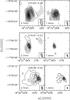 |
Fig. 1 Overlay of the PdBI maps of the 2.7 mm (left panels) and the 1.4 mm (right panels) continuum emission (contours) on the CH3CN (6–5) emission (grayscale) averaged under the K = 0, 1, 2, 3, and 4 components (left panels) and CH3CN (12–11) emission (grayscale) averaged under the K = 0, 1, 2, and 3 components (right panels) towards the cores G10.62–0.38, G19.61–0.23, and G29.96–0.02. The contour levels are 3, 9, 18, 27, 39, 51, and 75 times σ, where 1σ is 17 mJy beam-1 at 2.7 mm and 26.7 mJy beam-1 at 1.4 mm for G10.62−0.38, 6 mJy beam-1 at 2.7 mm and 33.3 mJy beam-1at 1.4 mm for G19.61−0.23, and 3 mJy beam-1 at 2.7 mm and 6.7 mJy beam-1 at 1.4 mm for G29.96−0.02. Grayscale levels are 3, 5, 10, 15, 20, 30, and 40 times (36 for G10) σ, where 1σ is 15 mJy beam-1 at 2.7 mm and 15 mJy beam-1 at 1.4 mm for G10, 30 mJy beam-1 at 2.7 mm and 50 mJy beam-1 at 1.4 mm for G19, and 15 mJy beam-1 at 2.7 mm and 65 mJy beam-1 at 1.4 mm for G29. The synthesized beam is shown in the lower righthand corner. The white cross marks the position of the 1.4 mm continuum emission peak. The source B seen towards G19.61−0.23 at 2.7 mm is the UC Hii region B observed by Furuya et al. (2005). |
Interferometric observations of G10, G19, and G29 were carried out with the IRAM Plateau de Bure Interferometer (PdBI) on February 28 and March 16, 2004, and on February 26 and March 21, 2005. G29 was observed in the most extended 8A) and compact (C) configurations while cores G19 and G10 were observed in the extended (B) and compact (C) ones. Owing to technical problems during the observations, the only usable configuration for G19 was the compact one, while for G10 it was the extended one. Table 2 reports the configurations used for each source and the synthesized beams. By using the dual frequency capabilities of the PdBI we observed simultaneously at 2.7 and 1.4 mm. The frequency setup of the correlator and the list of the observed molecular lines are shown in Table 3. The units of the correlator were placed in such a way that a frequency range free of lines could be used to measure the continuum flux. The phase centers used are indicated in Table 1. The bandpass of the receivers was calibrated by observations of the quasar 3C 273. Amplitude and phase calibrations were achieved by monitoring 1730–130 and 1741–038, whose flux densities were determined relative to MWC 349 or 1749+096. The flux densities estimated for 1730−130 are in the range 1.55–2.41 Jy at 2.7 mm and 0.78–1.71 Jy at 1.4 mm, while those for 1741–038 are in the range 3.57–3.80 Jy at 2.7 mm and 2.18–2.77 Jy at 1.4 mm. The uncertainty in the amplitude calibration is estimated to be ~20%. The data were calibrated and analyzed with the GILDAS1 software package developed at IRAM and Observatoire de Grenoble. The continuum maps were created from the line free channels. We subtracted the continuum from the line emission directly in the (u, v)-domain.
Positions, flux densities, and diameters of the cores.
4. Results
4.1. Continuum emission
Figure 1 shows the PdBI maps of the 2.7 and 1.4 mm continuum emission overlayed on the CH3CN (6–5) and CH3CN (12–11) emission towards the three cores. The position and fluxes at 2.7 and 1.4 mm, and the deconvolved size of the sources measured as the average diameter of the 50% contour at 1.4 mm, are given in Table 4. As seen below, the millimeter emission at 2.7 mm of the cores is highly contaminated by free-free emission of the nearby or embedded UC Hii region(s). Because the 1.4 mm emission is less affected by this problem and traces the HMC better, the positions given in Table 4 are those of the 1.4 mm emission peak.
4.1.1. G10.62−0.38
The continuum dust emission of G10, which is hardly resolved at 2.7 mm, shows a compact source plus an extended envelope. The peak of the emission at 1.4 mm coincides with the peak at 2.7 mm, and is very close to the position of the UC Hii region (see Fig. 1 of Sollins et al. 2005). As seen in Fig. 1, the continuum emission at 1.4 mm coincides with the CH3CN (12–11) emission. At this wavelength, the source is clearly resolved in the east-west direction, and shows an eastern elongation, associated with CH3CN emission, which suggests the presence of another embedded source. On the other hand, at 2.7 mm, the peak of the continuum emission is slightly displaced from the peak of the CH3CN (6–5) averaged emission. Although we cannot rule out the possibility of another embedded eastern source, the displacement of the line emission very likely occurs because the observations of this core have only been carried out with the extended configuration. Therefore, part of the extended line emission has been filtered out by the interferometer, making it very difficult to properly clean the dirty line maps.
To derive a rough estimate of the free-free contribution of the UC Hii region at millimeter wavelengths, we extrapolated the 1.3 cm emission measured by Sollins & Ho (2005) assuming optically thin free-free emission (Sν ∝ ν-0.1). The flux-integrated density at 1.3 cm is 2.5 Jy, and the expected free-free emission is ~2.14 Jy at 2.7 mm and ~2.00 Jy at 1.4 mm. Therefore, the dust continuum emission associated with the HMC is 0.28 Jy at 2.7 mm and 1.40 Jy at 1.4 mm (see Table 4). Klaassen et al. (2009) have estimated a thermal dust emission of 2 Jy at 1.4 mm. However, the free-free emission contribution at 1.4 mm estimated by these authors from radio recombination lines is less than half our estimate (0.92 Jy, P. D. Klaassen 2010, priv. comm.). The spectral index of the dust emission between 2.7 and 1.4 mm is 2.3, which corresponds to a power-law index β of the dust emissivity of 0.3. This value of β is very low and indicates that the contribution of the free-free emission at 2.7 mm is likely higher than estimated. Therefore, β should be taken as a lower limit.
4.1.2. G19.61–0.23
The nature of the continuum dust emission of G19 at 2.7 mm is clearly different from
that at 1.4 mm. The emission at 2.7 mm is dominated by the free-free emission of the
UC Hii regions embedded in the core (e.g. Furuya et al. 2005). As seen in Fig. 1, the
emission shows two clumps: the larger eastern one associated with the UC Hii
regions A, C, D, F, and J, with a morphology similar to the one mapped at 3.5 cm by
Furuya et al. (2005); and the smaller western one
associated with the UC Hii region B. The position and flux density of this
source at 2.7 mm are reported in Table 4. On the
other hand, the emission at 1.4 mm is clearly associated with the HMC, as traced by the
CH3CN (12–11) line emission. The HMC is also visible in CH3CN
(6–5) at 2.7 mm. This dichotomy between the emission at 2.7 and 1.4 mm is also reflected
in the position of the peak, which at 2.7 mm (α(J2000) =
18h27m38 13,
δ(J2000) = –11° 56′ 39
13,
δ(J2000) = –11° 56′ 39 3)
does not coincide with that at 1.4 mm (see Table 4).
3)
does not coincide with that at 1.4 mm (see Table 4).
The complexity of the free-free emission and the number of UC Hii regions embedded in the eastern core at 2.7 mm makes it very difficult to estimate the free-free emission contribution at millimeter wavelengths by extrapolating the centimeter emission. Instead, we estimated the dust continuum emission of the HMC by measuring the flux density in a region surrounding the HMC as traced by the CH3CN (6–5) line. The flux density at 2.7 mm is ~160 mJy, which is a value consistent with the 147 mJy measured by Furuya et al. (2005) at 3.3 mm. At 1.4 mm, the emission seems to be associated only with the HMC, so we assumed that the continuum emission is thermal dust (see Table 4). The spectral index of the HMC between 2.7 and 1.4 mm is 3.2, which corresponds to β = 1.2. Furuya et al. (2010) estimate β ≳ 0.7 between 3 mm and 890 μm, a value lower than but still consistent with our estimate.
4.1.3. G29.96–0.02
As for G19, in G29 the nature of the 2.7 mm continuum emission towards the core is not
the same as at 1.4 mm. At 2.7 mm, the emission is clearly contaminated by the cometary
UC Hii region, and it outlines the cometary arc seen in previous observations
at centimeter (e.g. Cesaroni et al. 1994) and
mid-infrared wavelengths (De Buizer et al. 2002).
Some emission is also visible in front of the arc, associated with the HMC traced by the
CH3CN (6–5) line and H2O maser emission (Hofner et al. 1996; Olmi et al. 2003). At 1.4 mm, the cometary arc is still visible, but the strongest
continuum emission is associated with the HMC traced by the CH3CN (12–11)
line emission in front of the arc. In fact, the peak at 2.7 mm
(α(J2000) =
18h46m0394,
δ(J2000) = –02° 39′ 219)
is shifted by  eastwards with respect to that at 1.4 mm (Table 4).
To obtain a rough estimate of the free-free contribution to the 2.7 mm continuum emission, we extrapolated the 1.3 cm emission measured by Cesaroni et al. (1994) to 2.7 mm assuming optically thin free-free emission. We measured the flux density at 1.3 cm inside a region that corresponds to the 3σ contour level of the 2.7 mm continuum emission and obtained a value of 2.74 Jy. Therefore, the expected free-free emission at 2.7 mm is ~2.35 Jy. This value is higher than the flux density measured at 2.7 mm (see Table 4). Given that the uv-coverages of the centimeter and millimeter observations are different, it is not surprising that the expected free-free emission value is higher than what is actually measured. It is evident that the emission at this wavelength is dominated by free-free emission. According to Olmi et al. (2003), who have estimated the contribution of the free-free emission at 2.7 mm by using the same uv-coverage and restoring beam at centimeter and millimeter wavelengths, the expected thermal dust contribution is ~0.15 Jy. Using the same method, Maxia et al. (2001) estimate a dust emission of 0.24 Jy at 3.4 mm, which shows the uncertainty of these measurements. At 1.4 mm, the emission from the HMC is clearly distinguishable from that of the cometary arc associated with the UC Hii region. Therefore, the continuum dust emission of the HMC has been estimated by measuring the flux density in a region surrounding it. The flux density of 0.83 Jy is slightly higher than the value of 0.56 Jy estimated at 1.3 mm by Maxia et al. (2001) after subtracting the free-free contribution. Maxia et al. (2001) mention that their flux density measurement at 1.3 mm is lower than expected and could be affected by spatial filtering of extended emission. After adopting the values of Olmi et al. (2003) at 2.7 mm and our estimate at 1.4 mm, one obtains a spectral index of 2.5, which corresponds to β = 0.5. This value of β is very low and indicates that the contribution of the free-free emission at 2.7 mm is likely to be higher than estimated. Therefore, β should be taken as a lower limit.
4.2. CH3CN
Maps of the CH3CN (6–5) emission averaged under the K = 0, 1, 2, 3, and 4 components and of the CH3CN (12–11) emission averaged under the K = 0, 1, 2, and 3 components towards G10, G19, and G29 are shown in Fig. 1. Figures 2–4 show the spectra of the CH3CN and CH313CN (12–11) and (6–5) lines towards the three cores. The first vibrational state above the ground of the CH3CN (6–5) line, which is denoted as v8 = 1, is also shown in the figures. The spectra have been obtained by averaging the emission inside the 3σ contour levels of the corresponding maps in Fig. 1.
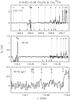 |
Fig. 2 Methyl cyanide spectra obtained by integrating the emission inside the 3σ contour level area at 2.7 and 1.4 mm towards G10 as seen with the PdBI. We show in the top CH3CN (12–11), in the middle CH3CN (6–5), and in the bottom CH3CN (6–5) vibrationally excited (v8 = 1). The different K-components (top and middle panels) are marked with dashed lines in the upper (lower) part of each spectra in the case of CH3CN (CH313CN). Different K-components of a same transition may have different spectral resolution because they were observed with different correlator units. Only the analyzed lines are labeled. |
 |
Fig. 5 Bottom panels: blueshifted (blue solid contours) and redshifted (red dashed contours) 13CO (1–0) (left) and 13CO (2–1) (right) averaged emission overlaid on the 1.4 mm continuum emission (grayscale) towards G19 and G29, respectively. The velocity intervals for which the blueshifted and redshifted emission have been averaged are indicated in blue and red dotted vertical lines in the corresponding upper spectra. Contour levels are 0.05, 0.1, 0.15, 0.2, 0.25, 0.3, and 0.35 Jy beam-1 (1σ ≃ 7 mJy beam-1) for the 13CO (1–0) blueshifted emission and 0.15, 0.2, 0.25, 0.3, and 0.35 Jy beam-1 (1σ ≃ 50 mJy beam-1) for the 13CO (1–0) redshifted emission (G19), and 0.03, 0.09, 0.15, 0.27, 0.39, and 0.51 Jy beam-1 (1σ ≃ 7 mJy beam-1) for the 13CO (2–1) blueshifted emission and 0.03, 0.06, 0.09, 0.15, 0.3 and 0.45 Jy beam-1 (1σ ≃ 7 mJy beam-1) for the 13CO (2–1) redshifted emission (G29). Grayscale contours for the continuum emission are the same as in Fig. 1. The synthesized beam is shown in the lower righthand corner. The white cross marks the position of the 1.4 mm continuum emission peak. Top panels: 13CO (1–0) and (2–1) spectra taken towards the 1.4 mm continuum emission peak of the G19 (left) and G29 (right) cores. The dashed vertical line indicates the systemic velocity of each core. |
Several K-components of the different rotational transitions of CH3CN and CH313CN at 1.4 and 2.7 mm are clearly detected towards the cores. Towards G10, only the K = 0−4 components of CH3CN (6–5) are visible. Several lines of CH3CN (6–5) v8 = 1 are also clearly detected towards G19 and G29 (Fig. 2), whereas only a few weak CH3CN (6–5) v8 = 1 lines are visible towards G10. As already mentioned in Sect. 4.1.1, the line emission of G10 at 2.7 mm could be severely affected by the extended emission having been resolved out.
As seen in Fig. 1, the CH3CN (12–11) emission is barely resolved in G19 and G29, and peaks at the same position as the 1.4 mm continuum emission. On the other hand, in G10, the CH3CN (12–11) emission is clearly resolved and shows two peaks: a western one associated with the 1.4 mm continuum emission peak and a weaker one to the east.
4.3. 13CO
We have clearly detected the 13CO (1–0) and (2–1) lines towards the cores (see Figs. 2–4). In G10, the line profiles exhibit a strong lack of emission at the center, probably due to a missing flux problem since the interferometer has filtered out part of the extended emission. Therefore, the 13CO emission has not been analyzed for this core.
Figure 5 shows the 13CO (1–0) and (2–1) spectra at the 1.4 mm continuum emission peak in G19 and G29. As seen in this figure, the 13CO spectra for these two cores are also affected by lack of emission at the central velocities. Although we cannot exclude the possibility that the lack of emission comes from a missing flux problem, that it is observed at redshifted velocities suggests that it could be due to absorption. This possibility is discussed in Sects. 5.3.2 and 5.3.3. In the bottom panels of Fig. 5, we present the maps of the 13CO (1–0) averaged blueshifted and redshifted emission with respect to the systemic velocity of G19 (41.6 km s-1) and of the 13CO (2–1) averaged blueshifted and redshifted emission with respect to the systemic velocity of G29 (98.9 km s-1) overlaid on the 1.4 mm continuum emission of each core. The 13CO emission traces a molecular outflow in each core: one oriented east-west in G19, and one oriented southeast-northwest in G29. The latter had been previously mapped in H2S by Gibb et al. (2004) and SiO by Beuther et al. (2007b). Taking the blueshifted and redshifted emission into account, the total extent of the outflows is ~14′′ (~0.86 pc) in G19 and ~6′′ (~0.10 pc) in G29.
5. Discussion
5.1. Temperature and mass estimates
CH3CN is a symmetric top molecule, so it can be used to estimate the
temperature in the cores. The rotational temperature, Trot,
and the total methyl cyanide column density,
NCH3CN, can be estimated by means of the rotation
diagram method, which assumes that the molecular levels are populated according to LTE
conditions at a single temperature Trot. In the high-density
limit where level populations are thermalized, one expects that
Trot = Tkin, the kinetic
temperature. The CH3CN ground-level transitions appear to be optically thick
for all cores, as suggested by the ratio between the main species and isotopomer.
Therefore, although in the Boltzmann plot we show all the measurements (see Fig. 6), the fit was only performed using the
 CN and vibrational excited CH3CN
transitions. All the spectra were obtained by averaging the emission inside the
3σ contour levels of the corresponding maps in Fig. 1. The values obtained at 1.4 mm were afterwards
corrected because the area used to average the emission was smaller than that of the
2.7 mm emission. The relative abundances
[CH3CN]/[CN] were estimated following Wilson &
Rood (1994), who give interstellar abundances as
a function of Galactocentric distance, and are 47, 44, and 50 for G10, G19, and G29,
respectively.
CN and vibrational excited CH3CN
transitions. All the spectra were obtained by averaging the emission inside the
3σ contour levels of the corresponding maps in Fig. 1. The values obtained at 1.4 mm were afterwards
corrected because the area used to average the emission was smaller than that of the
2.7 mm emission. The relative abundances
[CH3CN]/[CN] were estimated following Wilson &
Rood (1994), who give interstellar abundances as
a function of Galactocentric distance, and are 47, 44, and 50 for G10, G19, and G29,
respectively.
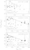 |
Fig. 6 Rotation diagram for G10, G19, and G29 with superimposed fit. Only the data for the CH313CN transitions and the CH3CN (6–5) v8 = 1 transition have been fitted. Filled circles, open circles, and filled triangles correspond to the CH313CN (6–5), the CH313CN (12–11), and the CH3CN (6–5) v8 = 1 transition, respectively. |
Figure 6 shows the rotational diagram, together with
the fits, and the estimated Trot and
NCH3CN for each core. The rotational
temperatures obtained with the fits are 87, 244, and 158 K for G10, G19, and G29,
respectively, while NCH3CN are 2 × 10¹⁵,
2 × 10¹⁵, and 1 × 1016 cm-2 for G10, G19, and G29.
Klaassen et al. (2009) have derived a temperature
of 323 ± 105 K for G10 using the rotational diagram method. This value is 4 times higher
than our estimated temperature. However, these authors use the optically thick
CH3CN (12–11) lines to derive Trot, so their
value should be taken as an upper limit. Wu et al. (2009) estimate a temperature of 552 K for G19 using the rotational diagram
method for CH3CN (18–17). This value is about 2.5 times higher than our
estimated temperature. This discrepancy is due to these authors using the optically thick
CH3CN lines in their calculations. In fact, Furuya et al. (2010), who only fit the optically thin
CN (18–17) lines in the rotation diagram,
have obtained a temperature estimate of 208 K, similar to our value. Finally, Olmi
et al. (2003) estimate a temperature of 150 K for
G29 by using the rotational diagram for CN (6–5) and vibrationally excited
CH3CN (6–5). This value of Trot is consistent
with our estimate.
Parameters of the toroids.
The masses of the HMCs have been estimated from the 1.4 mm dust continuum emission assuming a dust opacity of ≃0.8 cm2 g-1 at 1.4 mm (Ossenkopf & Henning 1994), a gas-to-dust ratio of 100, and a dust temperature equal to Trot. Table 5 gives the radius, R, and masses, Mgas, of the cores, along with Trot. We derived a mass of 82 M⊙ for G10. Klaassen et al. (2009) have estimated a mass of 136 M⊙ at 1.4 mm, assuming a dust opacity of ≃18.87 cm2 g-1 at 2400 GHz (Hildebrand 1983), a dust-to-gas mass ratio of 100, β = 1.5, a temperature of 323 K (Klaassen 2010, priv. comm.), and a distance of 6 kpc. Using the same parameters, we obtain a mass of 102 M⊙ at 1.4 mm.
Properties of the molecular outflows.
For G19, the estimated HMC mass is 415 M⊙. The core mass calculated at 900 μm by Wu et al. (2009) is 15 M⊙. These authors estimate the mass by assuming β = 1.5, a temperature of 552 K and a distance of 4 kpc; however, Furuya et al. (2010) estimate a mass of the HMC of 1300 M⊙ (1580 M⊙ taking the other two submillimeter sources in the region into account) at 900 μm for a dust opacity of ≃0.005 cm2 g-1 at 230 GHz (Preibisch et al. 1993), a dust-to-gas mass ratio of 100, β = 1, a temperature of 80 K, and a distance of 12.6 kpc. Using the same dust opacity index, temperature, and distance as Wu et al. (2009), the estimated dust mass would be 16 M⊙, whereas the mass would be 2142 M⊙ using the same parameters as those of Furuya et al. (2010). On the other hand, Furuya et al. (2005) have estimated a mass of 800 M⊙ from the dust emission at 3.3 mm, assuming a Preibisch et al. (1993) dust opacity law, β = 1.5, a temperature of 65 K, and a distance of 3.5 kpc. Using the same dust opacity law, temperature, and distance, we would obtain a mass of 245 M⊙ from the HMC dust emission at 2.7 mm. These discrepancies among the values give an idea of how uncertain the values of the dust masses are and how important it is to have an accurate estimate of the distance.
For G29, we derived an HMC mass of 28 M⊙. Maxia et al. (2001) estimate a mass of 2900 M⊙ at 3.4 mm, assuming a Preibisch et al. (1993) dust opacity law, a dust-to-gas mass ratio of 100, β = 2, a temperature of 83 K, and a distance of 6 kpc. Using the same opacity law, β coefficient, and distance, Olmi et al. (2003) estimate a mass of 320 M⊙ at 2.7 mm. This could indicate that the thermal dust flux estimated by Maxia et al. (2001) could still have some free-free contribution. Assuming the same opacity law, temperature, and distance, the gas mass estimated from our observations at 1.4 mm would be 270 M⊙.
5.2. Physical parameters of the CO outflows
Figure 5 shows the molecular outflows mapped in 13CO (1–0) towards G19 and 13CO (2–1) towards G29. The parameters of the outflows are given in Table 6. The parameters have not been corrected for inclination. The size of the lobes R, mass M, outflow mass loss rate Ṁout, momentum P, kinetic energy E, momentum rate in the outflows F, and dynamical timescale tout were derived from the 13CO emission for the velocity ranges indicated in Fig. 5 and in Table 6. The dynamical timescale of the blueshifted and redshifted lobes was estimated as tout = R/Vout, where Vout is the difference in absolute value between the maximum blueshifted or redshifted velocity and the systemic velocity (see Table 1). The tout of the outflow is the maximum dynamical timescale of the two lobes. The rest of the parameters were calculated for the blueshifted and redshifted lobes separately, and then added to obtain the total value. The [13CO]/[H2] abundance ratio was estimated following Wilson and Rood (1994), and assuming an [H2]/[CO] abundance ratio of 104 (e.g. Scoville et al. 1986). We assumed an excitation temperature, Tex, of 40 K. The values estimated for the G19 outflow are 1.7 (1.9) times lower (higher) if Tex is 20 K (80 K). On the other hand, the parameters of the G29 outflow are 1.4 (1.7) times smaller (higher) if Tex is 20 K (80 K).
As seen in Table 6, the values of M, P, and E of the G19 outflow are about 30–90 times higher than those of the G29 outflow. The values of Ṁout and F are comparable. The dynamical timescale of the G29 outflow is one order of magnitude smaller than for the G19 outflow. The range of values obtained for G19 and G29, especially the outflow masses, are consistent with those estimated through interferometric observations for other well-studied HMCs (e.g. Furuya et al. 2002, 2008). Regarding the mass loss rates, 10-4−10-3 M⊙ yr-1, the values are consistent with those found for other massive molecular outflows. Finally, the dynamical timescales of the outflows, ~104 yr, are consistent with the values estimated by Furuya et al. (2002, 2008).
5.3. Dense gas kinematics
In the past years, we have detected clear velocity gradients in more than 5 HMCs (Beltrán et al. 2004, 2005; Furuya et al. 2008) that have been interpreted, in most of the cases, as produced by rotating toroids oriented perpendicularly to the bipolar outflow driven by the massive YSO(s) embedded in the HMC. As already done to search for velocity gradients in the HMCs G24.78+0.08 and G31.41+0.31 (Beltrán et al. 2004, 2005), we simultaneously fitted multiple CH3CN (12–11) K-components, assuming identical line widths and fixing their separations to the laboratory values, at each position where CH3CN is detected. In this case, we fitted the K = 0, 1, 2, and 3 components simultaneously.
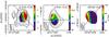 |
Fig. 7 Overlay of the PdBI CH3CN (12–11) emission averaged under the K = 0, 1, 2, and 3 components (contours) on the CH3CN (12–11) line peak velocity obtained with a Gaussian fit (colors) towards the cores G10 (left), G19 (middle), and G29 (right). The color levels in km s-1 are indicated in the wedge to the right of each panel. Contours for CH3CN (12–11) are the same as in Fig. 1. The straight line indicates the direction of the molecular outflow (Keto & Wood 2006; this paper). The synthesized beam is shown in the lower lefthand corner. |
Figure 7 shows the CH3CN (12–11) emission
averaged under the K = 0, 1, 2, and 3 components overlaid on the
CH3CN (12–11) line peak velocity obtained with the multiple Gaussian fits. As
seen in the LSR velocity maps (Fig. 7), all cores
show clear velocity gradients, with VLSR increasing steadily
along well-defined directions. As seen in the next sections, the most plausible
explanation for the velocity gradients observed in the HMCs is rotation. Therefore,
following Beltrán et al. (2004, 2005), we calculated the parameters of the rotating
toroids (see Table 5). The rotation velocity
Vrot, was estimated as half the velocity range measured in
the gradients. The virial mass Mvir was estimated from
CH3CN (12–11) by assuming a spherical clump with a power-law density
distribution ρ ∝ rp, with
p = 1.5, and neglecting contributions from the magnetic field and
surface pressure, and Mvir was computed following the
expression
Mvir = 0.407 d θCH3CN ΔV2,
where the distance d is in kpc, the angular diameter,
θCH3CN, in arcsec, and the
CH3CN (12–11) line width, ΔV, in km s-1. The values
given in Table 5 should be multiplied by 1.25 for a
homogeneous density distribution, p = 0, and by 0.75 for a density
distribution with p = 2. The dynamical mass
Mdyn was computed by assuming equilibrium between
centrifugal and gravitational forces from the expression
Mdyn = Vrot R/Gsin2i,
where i is the inclination angle of the toroid with respect to the plane
of the sky, assumed to be 90° for an edge on toroid. Because the inclination angle of the
toroids is unknown, we arbitrarily assumed i = 45°. The mass infall rate
was computed from the expression
Ṁinf = Mgas 2 Vinf/R
assuming that the infall velocity Vinf is equal to the
rotation velocity following Allen et al. (2003). We
estimated the lifetimes of the toroids in two different ways, one by measuring the infall
timescale tinf as
Mgas/Ṁinf, and the other one by
estimating the free-fall time tff. The values are given in
Table 5. The free-fall time was estimated from
the expression  yr (Eq. (3.5) of Hartmann 1998), where N, the number density of
molecular hydrogen gas, is
3 Mgas/4 π R3 2.8 mH.
The parameters of the rotating structures are consistent with those estimated by Beltrán
et al. (2004) for the toroids in G24.78+0.08 and
G31.41+0.31 (see their Table 1).
yr (Eq. (3.5) of Hartmann 1998), where N, the number density of
molecular hydrogen gas, is
3 Mgas/4 π R3 2.8 mH.
The parameters of the rotating structures are consistent with those estimated by Beltrán
et al. (2004) for the toroids in G24.78+0.08 and
G31.41+0.31 (see their Table 1).
5.3.1. G10.62–0.38
The CH3CN LSR velocity map towards G10 shows a clear velocity gradient with velocity increasing from SE to NW (Fig. 7). This velocity gradient has the same direction as that observed in NH3 by Sollins & Ho (2005), and more recently in SO2 by Klaassen et al. (2009), although the SO2 gradient is not as clear as the one seen in NH3 or in CH3CN. That the direction of the gradient is almost perpendicular to the direction of the molecular outflow observed towards this HMC (see Fig. 7; Keto & Wood 2006; Klaassen et al. 2009; López-Sepulcre et al. 2009) suggests that it is caused by the rotation of the core.
As seen in Table 5, Mgas and Mvir are comparable, suggesting that turbulence could support the toroid. On the other hand, Mgas is 2.5 times higher than Mdyn, suggesting that the toroid could be unstable. We note, however, that Mdyn has been calculated for an inclination angle i = 45° with respect to the plane of the sky. For i = 25°, the two become equal. The Ṁinf value is high, on the order of 10-2 M⊙ yr-1, but comparable to what has been found in other high-mass star-forming regions (Beltrán et al. 2004; Fontani et al. 2002). The tinf and tff timescales are consistent and a few 103 yr. Unfortunately, we have not been able to estimate the parameters of the outflow (see Sect. 4.3) to compare the timescale of the toroid with that of the outflow, or the infall rate with the mass loss rate.
5.3.2. G19.61–0.23
The CH3CN LSR velocity map towards G19 shows a clear velocity gradient with velocity increasing from S to N (Fig. 7). A similar velocity gradient has been observed in CH3CN (18–17) by Furuya et al. (2010). As seen in Fig. 5, the outflow associated with this HMC seems to be oriented approximately E-W. Therefore, as for G10, the most plausible explanation of this gradient is rotation.
As seen in Table 5, Mgas and Mvir are comparable, suggesting that turbulence, magnetic fields, and/or thermal pressure could support the toroid. On the other hand, Mgas is 30 times higher than Mdyn. Even if i were 10°, Mgas would still be almost 2 times greater. Therefore, this suggests that the G19 toroid is highly unstable, and it is probably undergoing collapse. Further evidence in favor of the collapse of this toroid is provided by 13CO (2–1). As mentioned in Sect. 4.3, the 13CO (2–1) transition for G19 is affected by absorption at redshifted velocities (see Fig. 5). A prominent inverse P-Cygni profile has also been observed in 13CO (3–2), C18O (3–2), and CN (3–2) with the Submillimeter Array (Wu et al. 2009; Furuya et al. 2010). The 13CO (3–2) line exhibits absorption from 41.5 to 48 km s-1, and the peak of the absorption is at 43.8 km s-1 (Wu et al. 2009). Such a profile is similar to the one observed by us in 13CO (2–1), for which the absorption is visible from 41.6 to 54.1 km s-1, and the peak is at 45.4 km s-1. Figure 8 shows the map of the 13CO (2–1) absorption averaged over the velocity interval 41.6–54.1 km s-1 overlayed on the 1.4 mm continuum emission. As seen in this figure, the absorption is well-correlated with the continuum emission, and the peak of the absorption coincides with that of the continuum emission.
Similar inverse P-Cygni profiles due to redshifted absorption against the dust continuum emission or an Hii region have already been observed towards other massive star-forming regions, such as G24.78+0.08 (Beltrán et al. 2006), G31.41+0.31 (Girart et al. 2009; Frau et al., in prep.) and W51 IRS2 (Zapata et al. 2008). In all cases, the redshifted absorption has been interpreted as the signature of infall towards the core center. The same interpretation has been proposed by Wu et al. (2009) and Furuya et al. (2010) for the inverse P-Cygni profiles observed in 13CO (3–2), C18O (3–2), and CN (3–2) towards G19. The 13CO (2–1) line brightness temperature (TB ≃ −10.9 K) measured along the line-of-sight towards the position of the HMC is comparable to the continuum brightness temperature (Tc ≃ 10.3 K). Hence, we have not been able to estimate the excitation temperature of the absorbing gas.
Considering that the systemic velocity VLSR of G19 is 41.6 km s-1 and that the peak of the redshifted absorption is at 45.4 km s-1, we estimated the infall velocity as Vinf = | VLSR–Vredshifted | = 3.8 km s-1, following Beltrán et al. (2006). The Vinf estimated from 13CO (3–2) is 3.5 km s-1 (Wu et al. 2009) and 4 km s-1 (Furuya et al. 2010), whereas from CN (3–2) it is 6.0 km s-1 (Wu et al. 2009). The Vinf estimated from the redshifted absorption is higher than the infall velocity used to estimate Ṁinf and tinf in Table 5, which is 1 km s-1. This value is a rough estimate of the infall velocity, so the discrepancy between the two Vinf estimates is not surprising. What this discrepancy indicates is that infall is stronger than rotation. Assuming Vinf = 3.8 km s-1, Ṁinf estimated from Mgas (see Sect. 5.3) is 0.1 M⊙ yr-1, and tinf = × 103 yr. This value is more similar to the estimated tff.
Following Beuther et al. (2002), one can estimate the mass accretion rate Ṁacc from the outflow mass loss rate Ṁout. According to these authors, the mass loss rate of the outflow is related to the mass loss rate of the internal jet entraining the outflow Ṁjet as Ṁout = Ṁjet Vjet/Vout, where the ratio between the jet velocity Vjet and the molecular outflow velocity Vout is ~20. Assuming a ratio between Ṁjet and the mass accretion rate onto the protostar Ṁacc of approximately 0.3 (Tomisaka 1998; Shu et al. 1999), one finds that Ṁout = 20 Ṁjet = 6 Ṁacc. Therefore, for G19, Ṁacc would be ~4 × 10⁻⁴ M⊙ yr-1. Ṁacc is about two orders of magnitude lower than Ṁinf (see Table 5). The outflow parameters have not been corrected for inclination, and Ṁout is to be multiplied by tani to correct for the inclination angle i of the flow with respect to the line-of-sight. However, a correction by a factor >10 would imply i > 84°, which seems very unlikely because rotation would be very difficult to detect in such a face-on structure. Therefore, the outflow inclination cannot account for the difference between Ṁacc and Ṁinf. In addition, part of the extended outflow emission could have been filtered out by the interferometer, and therefore Ṁout and Ṁacc should be considered as lower limits. However, after inspecting the 13CO channel maps, we conclude that the missing flux problem is unlikely to account for 2 orders of magnitude of difference in the estimates of the outflow parameters. Moreover, the single-dish study of López-Sepulcre et al. (2010) has obtained a similar result with mass accretion rates 2 to 4 orders of magnitude lower than the infall rates for a sample of high-mass cluster-forming clumps. Their interpretation is that Ṁinf represents the infall of the material onto a cluster of stars, while Ṁacc corresponds to the material being accreted onto a single massive star, responsible for the massive molecular outflow detected. The high masses and luminosities involved suggest that these rotating toroids likely host a stellar cluster rather than a single star (Beltrán et al. 2005; Cesaroni et al. 2006).
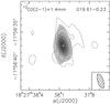 |
Fig. 8 Overlay of the 13CO (2–1) averaged absorption (dashed contours) on the 1.4 mm continuum emission (grayscale). The absorption has been averaged over the velocity interval 41.6–54.1 km s-1. Negative contours range from −0.1 to −0.7 Jy beam-1 in steps of −0.1 Jy beam-1 (1σ ≃ 0.03 Jy beam-1). Grayscale contours for the continuum emission are the same as in Fig. 1. The white cross marks the position of the 1.4 mm continuum emission peak. The synthesized beam is shown in the lower righthand corner. |
5.3.3. G29.96–0.02
The CH3CN LSR velocity map towards G29 shows a clear velocity gradient with velocity increasing in from W to E (Fig. 7). Cesaroni et al. (1998) and Olmi et al. (2003) have detected in NH3 and CH3CN a velocity gradient across the HMC approximately along the same direction by fitting the peak of the emission at each spectral channel. This is similar to the velocity gradient observed in HN13C by Beuther et al. (2007b). As seen in Fig. 5, the embedded YSO(s) in this HMC powers a molecular outflow with an SE-NW direction. This outflow has also been mapped in H2S (Gibb et al. 2004) and SiO (8–7) (Beuther et al. 2007b). The velocity gradient is clearly not perpendicular to the molecular outflow. Also for G10 and G19, the velocity gradients are not exactly perpendicular to the molecular outflows (see Fig. 7), although for these HMCs the discrepancy is only a few degrees. One possible explanation for the non-perpendicularity of the velocity gradient could be the highly elliptical beam of the PdBI observations. According to Guilloteau & Dutrey (1998), to analyze the velocity field, it is essential to use a circular beam, otherwise velocity gradients in marginally resolved objects may be severely distorted. To investigate this effect, we re-analyzed the OVRO CH3CN (6–5) observations towards G29 carried out by Olmi et al. (2003), with the simultaneous fit of the CH3CN K-components. Figure 9 shows the CH3CN (6–5) emission averaged under the K = 0 and 1 components overlaid on the CH3CN (6–5) line peak velocity. As seen in this plot, the synthesized beam of these observations is almost circular, and the velocity gradient shows an SW-NE direction. This direction is perpendicular to the molecular outflow, so we interpret the velocity gradient as due to rotation.
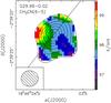 |
Fig. 9 Overlay of the OVRO CH3CN (6–5) emission from Olmi et al. (2003) averaged under the K = 0 and 1 components (contours) on the CH3CN (6–5) line peak velocity obtained with a Gaussian fit (colors) towards the core G29. The color levels in kilometers per second are indicated in the wedge to the right. Contours for CH3CN (6–5) are range from 0.1 to 0.7 Jy beam-1 in steps of 0.1 Jy beam-1 (1σ ≃ 0.03 Jy beam-1). The straight line indicates the direction of the molecular outflow. The synthesized beam is shown in the lower lefthand corner. |
As seen in Table 5, Mvir is 6 times higher than Mgas, suggesting that turbulence, magnetic fields, and/or thermal pressure could support the toroid. On the other hand, Mgas is 2 times higher than Mdyn. For i ~ 30°, the two become comparable. The difference between Mgas and Mdyn could suggest that the G29 toroid is unstable and probably undergoing collapse. As mentioned in Sect. 4.3, the 13CO (2–1) transition towards the G29 HMC is affected by absorption at redshifted velocities (see Fig. 5). In this case, the absorption is less clear than for G19. Probably this is because emission and absorption are mixed along the line-of-sight towards the HMC, making the latter less evident. The peak of the absorption is at ~104 km s-1, therefore Vinf is ~5 km s-1. The Vinf estimated from the redshifted absorption is higher than the infall velocity used to estimate Ṁinf and tinf in Table 5, which is 1.6 km s-1. Assuming Vinf = 5 km s-1, Ṁinf estimated from Mgas (see Sect. 5.3) is 0.03 M⊙ yr-1, and tinf = 1 × 10³ yr. As already seen for the other toroids, Ṁinf is high, on the order of 10-2 M⊙ yr-1, but comparable to what has been found in other high-mass star-forming regions. The tinf and tff timescales are consistent and ~103 yr.
The mass accretion rate Ṁacc estimated from the outflow mass loss rate Ṁout (see previous section) is ~8 × 10⁻⁵ M⊙ yr-1. As for G19 (see previous section), the accretion rate is two orders of magnitude lower than the infall rate (see Table 5), and neither the inclination of the outflow nor the filtering out of the emission seem able to account for such a discrepancy. Therefore, also in this case, the most plausible explanation for Ṁinf ≫ Ṁacc is that the material of the toroid is infalling onto a cluster of stars instead of a single star, which is responsible for the molecular outflow.
5.3.4. Absorption towards the G29.96–0.02 UC HII region
Maxia et al. (2001) detect redshifted absorption in the integrated spectra of HCO+ (1–0) towards G29. The map of the HCO+ (1–0) line averaged over the absorption velocity range, 99–102 km s-1, shows that the absorption is positionally coincident with the UC Hii region (see Fig. 8 of Maxia et al. 2001). To check whether this absorption is also visible in the 13CO (2–1) line, we obtained the spectrum towards the peak of the 1.4 mm continuum emission of the UC Hii region and, following Maxia et al. (2001), over the 3σ contour level of the 1.4 mm continuum emission towards G29, that is, a region including the HMC and the UC Hii region (Fig. 10). As seen in the top panel of this figure, deep and broad absorption is clearly visible towards the UC Hii region. When integrating the 13CO (2–1) emission over the 3σ contour level of the 1.4 mm continuum emission, the emission combines with the absorption, making it less pronounced. However, the absorption is still clearly visible at a velocity of ~104 km s-1. This velocity is different from that of the HCO+ absorption, which is 98.8 km s-1 according to Maxia et al. (2001). This may mean that this 13CO absorption feature is not real but due to the interferometer resolving out extended emission at this velocity. Alternatively, the 13CO emission could be stronger and more extended than the HCO+ emission, and the combination of emission and absorption could thus produce an absorption feature at a different velocity interval from what is observed in HCO+. From Fig. 10 and the 13CO (2–1) channel maps, one sees that the redshifted absorption is visible towards the position of the UC Hii region in the velocity range 98.9–105.9 km s-1. The 13CO (2–1) map averaged over this velocity interval is shown in Fig. 11. This map is similar to the HCO+ integrated map of Maxia et al. (2001) and clearly shows absorption towards the UC Hii region, whereas emission is visible towards the HMC and towards the NE of the UC Hii region. For these reasons, we believe that the 13CO absorption feature at ~104 km s-1 is real, although only complementary single-dish data may prove this.
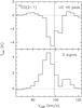 |
Fig. 10 13CO (2–1) integrated spectra towards the peak of the 1.4 mm continuum emission of the UC Hii region (top), and over the 3σ contour level of the 1.4 mm continuum emission (bottom) towards G29. The dashed vertical line indicates the systemic velocity of each core. |
The 13CO (2–1) line brightness temperature TB measured along the line-of-sight towards the position of the UC Hii region is –4.5 K. Within the uncertainties, this is comparable to the continuum brightness temperature Tc ≃ 3.4 K, which shows that the continuum photons are almost totally absorbed by the 13CO gas.
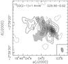 |
Fig. 11 Overlay of the 13CO (2–1) mean absorption (dashed contours) on the 1.4 mm continuum emission (grayscale). The absorption has been averaged over the velocity interval 98.9–105.9 km s-1. Negative contours are –0.06 and −0.12 Jy beam-1, while positive contours range from 0.08 to 0.56 in steps of 0.08 Jy beam-1 (1σ ≃ 0.02 Jy beam-1). Grayscale contours for the continuum emission are the same as in Fig. 1. The synthesized beam is shown in the lower righthand corner. |
6. Rotating toroids in massive star-forming regions
In recent years several massive, rotating structures have been discovered in high-mass YSOs (see Table 7). Following Cesaroni et al. (2006), these rotating structures should be classified into two classes on the basis of the ratio between the mass of the rotating structure and that of the star. On the one hand, rotating structures with masses lower than the mass of the central, star, typically found around B-type stars, are centrally supported disks. On the other hand, structures with masses in excess of several 10 M⊙, much greater than the mass of the central star(s), and found around O-type stars, should be called toroids.
In Beltrán et al. (2004, 2005) and this work, we have concentrated on the study of the large rotating toroids around O-type stars, deriving their properties and comparing them to disks around low-mass YSOs. The sizes of the toroids are several 1000 AU, which are an order of magnitude higher than those of accretion disks in solar-type pre-main sequence stars (~a few 100 AU). As already discussed, their masses are much higher than the mass of any central (proto)star. In fact, these toroids are so huge that they may host not just a single star, but a whole cluster. This is completely different from the low-mass scenario, where the disks have masses of a few 10-3 to 10-1 M⊙ (Natta 2000), i.e. 10–100 times lower than the mass of the central star.
For some of the HMCs hosting rotating toroids, inverse P-Cygni profiles (or redshifted absorption) have also been detected (this work; Sollins et al. 2005; Beltrán et al. 2006; Zapata et al. 2008; Girart et al. 2009; Wu et al. 2009; Furuya et al. 2010), indicating that these toroids are not only rotating but also infalling. However, one sees that the infall rates range from 10-3 to 10-2 M⊙ yr-1, while those derived for accretion disks in low-mass YSOs range from 10-9 to 10-6 M⊙ yr-1 (Hartmann 1998).
Based on this and on the fact that the infall rates are 2 orders of magnitudes greater than the mass accretion rates estimated from the mass loss rates of the corresponding outflows (Sects. 5.3.2 and 5.3.3), we propose a scenario in which massive toroids would be transient structures infalling towards a central cluster of forming stars. In this scenario, the circumcluster toroids would be fed by a larger scale reservoir of material, consisting of the parsec-scale clumps surrounding them. The material of the toroids would infall onto the circumstellar disks in the cluster, and then from the disks it would accrete onto the corresponding central stars. In this sense, the circumcluster toroids would be the high-mass analogs of the circumstellar infalling envelopes surrounding low-mass stars, and the embedded circumstellar disks (not imaged yet towards O-type stars, Cesaroni et al. 2006, 2007) would correspond to the accretion disks observed towards Class 0 and I low-mass YSOs.
The differences in the velocity field observed towards low- and high-mass YSOs also support this idea that toroids are qualitatively different from disks. For low-mass stars, the disks undergo Keplerian rotation, while for toroids, Keplerian rotation is not possible on scales of 104 AU because the gravitational potential of the system is dominated by the massive toroid, not by the star. For this reason, it has been proposed that these toroids never reach equilibrium (Cesaroni et al. 2006). They could be transient entities, with timescales close to the free-fall time, ~104 yr. In contrast, according to Natta (2000), low-mass pre-main-sequence disks may live as long as 107 yr. To study the stability of these structures, we have plotted in Fig. 12 the tff/trot ratio versus Mgas, where the free-fall time tff is proportional to the dynamical timescale needed to refresh the material of the toroid and trot is the rotational period at the outer radius, 2 π R/Vrot, for a number of disks and toroids around high-mass (proto)stars. The gas masses found in the literature were estimated by assuming different dust opacity laws, and as seen in Sect. 5.1, this is an important source of uncertainty in the mass determination. Therefore, for all but one case (GH2O 92.67+3.072), we re-calculated the gas masses from the dust continuum emission using the dust opacities of Ossenkopf & Henning (1994), with a dust opacity of ≃0.8 cm2 g-1 at 1.4 mm, i.e. the same as used for our sources. We give this in Col. 3 of Table 7, while in col. 4 we give the mass estimates found in the literature. For those wavelengths for which the opacity has not been tabulated by Ossenkopf & Henning (1994), we extrapolated the value from λ = 1.4 mm assuming β = 2. These gas masses were used to estimate tff, which together with trot were calculated following Sect. 5.3 and using the parameters reported in Table 7. Assuming an uncertainty of ~20% in Mgas, Vrot, and R, the uncertainty in tff/trot would be ~25%. In all cases, if the structure rotates fast, the infalling material has enough time to settle into a centrifugally supported disk; vice versa, if the structure rotates slowly, the infalling material does not have enough time to reach centrifugal equilibrium and the rotating structure is a transient toroid. Therefore, the higher the tff/trot ratio, the more similar the rotating structure should be to a circumstellar disk. In fact, in Fig. 12, one sees that the less massive structures, which have masses comparable to or lower than that of the central star have the higher tff/trot ratio, while the massive toroids have a lower ratio. A typical example of a circumstellar disk in Keplerian rotation around a B-type star is the one found towards IRAS 20126+4104 (Cesaroni et al. 2005), while a typical example of rotating toroid around an O-type star is G31.41+0.31 (Beltrán et al. 2004, 2005).
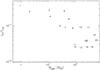 |
Fig. 12 Free-fall timescale to rotational period ratio versus gas mass of known rotating disks or toroids. The masses have been estimated assuming the dust opacities of Ossenkopf & Henning (1994). The numbers correspond to the entries of Table 7. |
In summary, our findings suggest that massive stars could form by infall/accretion through rotating toroids/disks, although the sizes, masses, timescales, infall, and accretion rates involved are much greater than those of low-mass accretion disks. It is important to stress that, although rotation, infall, and outflow have been detected towards massive YSOs, so far no real accretion disk in O-type stars has been imaged yet. However, as already discussed by Cesaroni et al. (2006), real accretion disks might be embedded inside the rotating toroids, and impossible to disentangle from the massive toroids with current instrumentation. Only the new capabilities of the Atacama Large Millimeter Array (ALMA), in terms of sensitivity and resolution, will shed some light on this important issue.
List of rotating disks and toroids in high-mass (proto)stars.
7. Conclusions
We analyzed millimeter high-angular resolution data, obtained with the IRAM PdBI interferometer, of the dust and gas emission towards the HMCs G10.62−0.38, G19.61−0.23, and G29.96−0.02. The aims were to study the structure of the cores, map the molecular outflows powered by the YSOs embedded in the HMCs, and reveal possible velocity gradients indicative of rotation.
The continuum emission at 2.7 mm is clearly dominated by free-free emission from the UC Hii region(s), while at 1.4 mm dust emission from the HMCs prevails.
The CH3CN (12–11) LSR velocity maps reveal clear velocity gradients in the three HMCs oriented perpendicular to the direction of the corresponding bipolar outflows. The gradients are interpreted as rotation. The gas temperatures, used to derive the mass of the cores, were obtained by means of the rotational diagram method, and are in the range of 87–244 K. The diameters and masses of the toroids lie in the range of 4550–12 600 AU and 28–415 M⊙, respectively.
The masses of the cores are comparable to the corresponding virial masses, suggesting that turbulence could support the toroids. Given that the dynamical mass is considerably lower than the mass of the cores, we suggest that the toroids are not centrifugally supported and are possibly undergoing collapse. For G19 and G29, this is also suggested by the redshifted absorption seen in 13CO (2–1). We infer that infall onto the embedded (proto)stars proceeds with rates of ~10-2 M⊙ yr-1 and on timescales of ~4 × 10³–104 yr. The infall rates derived for G19 and G29 are two orders of magnitude greater than the accretion rates indirectly estimated from the mass loss rate of the corresponding outflows. This suggests that the material in the toroids is not infalling onto a single massive star, which would be responsible for the corresponding molecular outflow, but onto a cluster of stars.
The masses, sizes, and infall rates of the rotating toroids are orders of magnitude higher than those of real accretion disks around lower mass stars, while their lifetimes are much shorter. Also, we find that the higher the mass of the rotating structure, the lower the tff/trot ratio. Therefore, circumstellar disks around B-type stars are centrifugally supported and undergo Keplerian rotation, while massive toroids around O-type stars appear to be transient structures undergoing collapse.
The GILDAS package is available at http://www.iram.fr/IRAMFR/GILDAS
The mass of this core has been estimated from CS emission (Bernard et al. 1999).
Acknowledgments
We thank the staff of IRAM for their help during the observations and data reduction.
References
- Allen, A., Li, Z.-Y., & Shu, F. H. 2003, ApJ, 599, 363 [NASA ADS] [CrossRef] [Google Scholar]
- Arce, H. G., Santiago-García, J., Jörgensen, J. K., et al. 2008, A&A, 681, L21 [Google Scholar]
- Argon, A. L., Reid, M. J., & Menten, K. M. 2000, ApJS, 129, 159 [NASA ADS] [CrossRef] [Google Scholar]
- Beltrán, M. T., Cesaroni, R., Neri, R., et al. 2004, ApJ, 601, L187 [NASA ADS] [CrossRef] [Google Scholar]
- Beltrán, M. T., Cesaroni, R., Neri, R., et al. 2005, A&A, 435, 901 [NASA ADS] [CrossRef] [EDP Sciences] [Google Scholar]
- Beltrán, M. T., Cesaroni, R., Codella, C., et al. 2006, Nature, 443, 427 [NASA ADS] [CrossRef] [PubMed] [Google Scholar]
- Bernard, J. P., Dobashi, K., & Momose, M. 1999, A&A, 350, 197 [Google Scholar]
- Beuther, H., Schilke, P., Sridharan, T. K., et al. 2002, A&A, 383, 892 [NASA ADS] [CrossRef] [EDP Sciences] [Google Scholar]
- Beuther, H., Zhang, Q., Sridharan, T. K., & Chen, Y. 2005, ApJ, 628, 800 [NASA ADS] [CrossRef] [Google Scholar]
- Beuther, H., Churchwell, E. B., McKee, C. F., & Tan, J. C. 2007a, in Protostars & Planets V, ed. B. Reipurth, D. Jewitt, & K. Keil (University of Arizona Press), 165 [Google Scholar]
- Beuther, H., Zhang, Q., Bergin, E. A., et al. 2007b, A&A, 468, 1045 [NASA ADS] [CrossRef] [EDP Sciences] [Google Scholar]
- Beuther, H., Zhang, Q., Hunter, T. R., et al. 2007c, A&A, 473, 493 [NASA ADS] [CrossRef] [EDP Sciences] [Google Scholar]
- Beuther, H., Walsh, A. J., Thorwirth, S., et al. 2008, A&A, 481, 169 [NASA ADS] [CrossRef] [EDP Sciences] [Google Scholar]
- Bonnell, I. A., Vine, S. G., & Bate, M. R. 2004, MNRAS, 349, 735 [NASA ADS] [CrossRef] [Google Scholar]
- Bonnell, I. A., Larson, R. B., & Zinnecker, H. 2007, in Protostars & Planets V, ed. B. Reipurth, D. Jewitt, & K. Keil (University of Arizona Press), 149 [Google Scholar]
- Blum, R. D., Damineli, A., & Conti, P. S. 2001, AJ, 121, 3149 [NASA ADS] [CrossRef] [Google Scholar]
- Cesaroni, R., Churchwell, E., Hofner, P., et al. 1994, A&A, 288, 903 [NASA ADS] [Google Scholar]
- Cesaroni, R., Hofner, P., Walmsley, C. M., & Churchwell, E. 1998, A&A, 331, 709 [NASA ADS] [Google Scholar]
- Cesaroni, R., Felli, M.,Jenness, T., et al. 1999, A&A, 345, 949 [NASA ADS] [Google Scholar]
- Cesaroni, R., Neri, R., Olmi, L., et al. 2005, A&A, 434, 1039 [NASA ADS] [CrossRef] [EDP Sciences] [Google Scholar]
- Cesaroni, R., Galli, D., Lodato, G., et al. 2006, Nature, 444, 703 [NASA ADS] [CrossRef] [PubMed] [Google Scholar]
- Cesaroni, R., Galli, D., Lodato, G., et al. 2007, in Protostars & Planets V, ed. B. Reipurth, D. Jewitt, & K. Keil (University of Arizona Press), 197 [Google Scholar]
- Codella, C., Benedettini, M., Beltrán, M. T., et al. 2009, A&A, 507, L25 [NASA ADS] [CrossRef] [EDP Sciences] [Google Scholar]
- De Buizer, J. M., Watson, A. M., Radomski, J. T., Piña, R. K., & Telesco, C. M. 2002, ApJ, 564, L101 [NASA ADS] [CrossRef] [Google Scholar]
- Fontani, F., Cesaroni, R., Caselli, P., & Olmi, L. 2002, A&A, 389, 603 [NASA ADS] [CrossRef] [EDP Sciences] [Google Scholar]
- Forster, J. R., & Caswell, J. L. 1989, A&A, 213, 339 [NASA ADS] [Google Scholar]
- Furuya, R. S., Cesaroni, R., Codella, C., et al. 2002, A&A, 390, L1 [NASA ADS] [CrossRef] [EDP Sciences] [Google Scholar]
- Furuya, R. S., Cesaroni, R., Takahashi, S., et al. 2005, ApJ, 624, 827 [NASA ADS] [CrossRef] [Google Scholar]
- Furuya, R. S., Cesaroni, R., Takahashi, S., et al. 2008, ApJ, 673, 363 [NASA ADS] [CrossRef] [Google Scholar]
- Furuya, R. S., Cesaroni, R., & Shinnaga, H. 2010, A&A, in press [Google Scholar]
- Galván-Madrid, R., Keto, E., Zhang, Q., et al. 2009, ApJ, 706, 1036 [NASA ADS] [CrossRef] [Google Scholar]
- Garay, G., Reid, M. J., & Moran, J. M. 1985, ApJ, 289, 681 [NASA ADS] [CrossRef] [Google Scholar]
- Garay, G., Moran, J. M., Rodríguez, L. F., & Reid, M. J. 1998, ApJ, 492, 635 [NASA ADS] [CrossRef] [Google Scholar]
- Gibb, A. G., Wyrowski, F., & Mundy, L. G. 2004, ApJ, 616, 301 [NASA ADS] [CrossRef] [Google Scholar]
- Girart, J. M., Beltrán, M. T., Zhang, Q., et al. 2009, Science, 324, 1408 [NASA ADS] [CrossRef] [PubMed] [Google Scholar]
- Guilloteau, S., & Dutrey, D. 1998, A&A, 339, 467 [NASA ADS] [Google Scholar]
- Hartmann, L. 1998, in Accretion Processes in Star Formation, Cambridge Astrophysics Ser., 32 [Google Scholar]
- Hildebrand, R. H. 1983, QJRAS, 24, 267 [NASA ADS] [Google Scholar]
- Ho, P. T. P., & Haschick, A. D. 1986, ApJ, 304, 501 [NASA ADS] [CrossRef] [Google Scholar]
- Hoffman, I. M., Goss, W. M., Palmer, P., & Richards, A. M. S. 2003, ApJ, 598, 1061 [NASA ADS] [CrossRef] [Google Scholar]
- Hofner, P., & Churchwell, E. 1996, A&AS, 120, 283 [NASA ADS] [CrossRef] [EDP Sciences] [Google Scholar]
- Hunter, T. R., Brogan, C. L., Megeath, S. T., et al. 2006, ApJ, 649, 888 [NASA ADS] [CrossRef] [Google Scholar]
- Keto, E. 2002, ApJ, 568, 754 [NASA ADS] [CrossRef] [Google Scholar]
- Keto, E., & Wood, K. 2006, ApJ, 637, 850 [NASA ADS] [CrossRef] [Google Scholar]
- Keto, E. R., Ho, P. T. P., & Reid, M. J. 1987, ApJ, 323, L117 [NASA ADS] [CrossRef] [Google Scholar]
- Keto, E. R., Ho, P. T. P., & Haschick, A. D. 1988, ApJ, 324, 920 [NASA ADS] [CrossRef] [Google Scholar]
- Klaassen, P. D., Wilson, C. D., Keto, E. R., & Zhang, Q. 2009, ApJ, 703 1308 [Google Scholar]
- Kolpak, M. A., Jackson, J. M., Bania, T. M., et al. 2003, ApJ, 582, 756 [NASA ADS] [CrossRef] [Google Scholar]
- Krumholz, M. R., Klein, R. I., McKee, C. F., Offner, S. S. R., & Cunningham, A. J. 2009, Science, 323, 754 [NASA ADS] [CrossRef] [PubMed] [Google Scholar]
- Kuiper, R., Klahr, H., Beuther, H., & Henning, T. 2010, ApJ, 722, 1556 [CrossRef] [Google Scholar]
- López-Sepulcre, A., Codella, C., Cesaroni, R., et al. 2009, A&A, 499, 811 [NASA ADS] [CrossRef] [EDP Sciences] [Google Scholar]
- López-Sepulcre, A., Cesaroni, R., & Walmsley, C. M. 2010, A&A, in press [Google Scholar]
- Maxia, C., Testi, L., Cesaroni, R., & Walmsley, C. M. 2001, A&A, 371, 287 [NASA ADS] [CrossRef] [EDP Sciences] [Google Scholar]
- McKee, C. F., & Tan, J. C. 2002, Nature, 416, 59 [NASA ADS] [CrossRef] [PubMed] [Google Scholar]
- McKee, C. F., & Tan, J. C. 2003, ApJ, 585, 850 [NASA ADS] [CrossRef] [MathSciNet] [Google Scholar]
- Natta, A. 2000 in Infrared space astronomy, today and tomorrow. ed. F. Casoli, J. Lequeux, & F. David, Les Houches Summer School, 70, 193 [Google Scholar]
- Olmi, L., Cesaroni, R., Hofner, P., et al. 2003, A&A, 407, 225 [NASA ADS] [CrossRef] [EDP Sciences] [Google Scholar]
- Ossenkopf, V., & Henning, Th. 1994, A&A, 291, 943 [NASA ADS] [Google Scholar]
- Patel, N., Curiel, S., Sridharan, T. K., et al. 2005, Nature, 437, 109 [NASA ADS] [CrossRef] [PubMed] [Google Scholar]
- Plume, R., Jaffe, D. T., & Evans, N. J. II 1992, ApJS, 78, 505 [NASA ADS] [CrossRef] [Google Scholar]
- Pratap, P., Megeath, S. T., & Bergin, E. A. 1999, ApJ, 517, 799 [NASA ADS] [CrossRef] [Google Scholar]
- Preibisch, Th., Ossenkopf, V., Yorke, H. W., & Henning, Th. 1993, A&A, 279, 577 [NASA ADS] [Google Scholar]
- Remijan, A., Shiao, Y.-S., Friedel, D. N., et al. 2004, ApJ, 617, 384 [NASA ADS] [CrossRef] [Google Scholar]
- Sandell, G., Wright, M., & Forster, J. R. 2003, ApJ, 590, L45 [NASA ADS] [CrossRef] [Google Scholar]
- Shi, H., Zhao, J.-H., & Han, J. L. 2010, ApJ, 710, 843 [NASA ADS] [CrossRef] [Google Scholar]
- Shu, F. H., Allen, A., Shang., H., et al. 1999, in The Origins of Stars and Planetary Systems, ed. C. J. Lada, & N. D. Kylafis (Kluwer Academic Press), 193 [Google Scholar]
- Scoville, N. Z., Sargent, A. I., Sanders, D. B., et al. 1986, ApJ, 303, 416 [NASA ADS] [CrossRef] [Google Scholar]
- Sollins, P. K., & Ho, P. T. P. 2005, ApJ, 630, 987 [NASA ADS] [CrossRef] [Google Scholar]
- Sollins, P. K., Zhang, Q., Keto, E., & Ho, P. T. P. 2005, ApJ, 624, L49 [NASA ADS] [CrossRef] [Google Scholar]
- Tomisaka, K. 1998, ApJ, 502, L163 [NASA ADS] [CrossRef] [Google Scholar]
- Walsh, A. J., Burton, M. G., Hyland, A. R., & Robinson, G. 1998, MNRAS, 301, 640 [NASA ADS] [CrossRef] [Google Scholar]
- Wilson, T. L., & Rood, R. T. 1994, ARA&A, 86, 317 [Google Scholar]
- Wood, D. O. S., & Churchwell, E. 1989, ApJS, 69, 831 [NASA ADS] [CrossRef] [Google Scholar]
- Wu, Y., Qin, S.-L., Guan, X., et al. 2009, ApJ, 697, L116 [NASA ADS] [CrossRef] [Google Scholar]
- Zapata, L. A., Palau, A., & Ho, P. T. P. 2008, ApJ, 479, L25 [Google Scholar]
- Zhang, Q., & Ho, P. T. P. 1997, ApJ, 488, 241 [NASA ADS] [CrossRef] [Google Scholar]
- Zhang, Q., Sridharan, T. K., Hunter, T. R., et al. 2007, A&A, 470, 269 [NASA ADS] [CrossRef] [EDP Sciences] [Google Scholar]
All Tables
All Figures
|
Fig. 1 Overlay of the PdBI maps of the 2.7 mm (left panels) and the 1.4 mm (right panels) continuum emission (contours) on the CH3CN (6–5) emission (grayscale) averaged under the K = 0, 1, 2, 3, and 4 components (left panels) and CH3CN (12–11) emission (grayscale) averaged under the K = 0, 1, 2, and 3 components (right panels) towards the cores G10.62–0.38, G19.61–0.23, and G29.96–0.02. The contour levels are 3, 9, 18, 27, 39, 51, and 75 times σ, where 1σ is 17 mJy beam-1 at 2.7 mm and 26.7 mJy beam-1 at 1.4 mm for G10.62−0.38, 6 mJy beam-1 at 2.7 mm and 33.3 mJy beam-1at 1.4 mm for G19.61−0.23, and 3 mJy beam-1 at 2.7 mm and 6.7 mJy beam-1 at 1.4 mm for G29.96−0.02. Grayscale levels are 3, 5, 10, 15, 20, 30, and 40 times (36 for G10) σ, where 1σ is 15 mJy beam-1 at 2.7 mm and 15 mJy beam-1 at 1.4 mm for G10, 30 mJy beam-1 at 2.7 mm and 50 mJy beam-1 at 1.4 mm for G19, and 15 mJy beam-1 at 2.7 mm and 65 mJy beam-1 at 1.4 mm for G29. The synthesized beam is shown in the lower righthand corner. The white cross marks the position of the 1.4 mm continuum emission peak. The source B seen towards G19.61−0.23 at 2.7 mm is the UC Hii region B observed by Furuya et al. (2005). |
| In the text | |
|
Fig. 2 Methyl cyanide spectra obtained by integrating the emission inside the 3σ contour level area at 2.7 and 1.4 mm towards G10 as seen with the PdBI. We show in the top CH3CN (12–11), in the middle CH3CN (6–5), and in the bottom CH3CN (6–5) vibrationally excited (v8 = 1). The different K-components (top and middle panels) are marked with dashed lines in the upper (lower) part of each spectra in the case of CH3CN (CH313CN). Different K-components of a same transition may have different spectral resolution because they were observed with different correlator units. Only the analyzed lines are labeled. |
| In the text | |
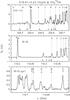 |
Fig. 3 Same as Fig. 2 for G19. |
| In the text | |
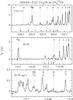 |
Fig. 4 Same as Fig. 2 for G29. |
| In the text | |
|
Fig. 5 Bottom panels: blueshifted (blue solid contours) and redshifted (red dashed contours) 13CO (1–0) (left) and 13CO (2–1) (right) averaged emission overlaid on the 1.4 mm continuum emission (grayscale) towards G19 and G29, respectively. The velocity intervals for which the blueshifted and redshifted emission have been averaged are indicated in blue and red dotted vertical lines in the corresponding upper spectra. Contour levels are 0.05, 0.1, 0.15, 0.2, 0.25, 0.3, and 0.35 Jy beam-1 (1σ ≃ 7 mJy beam-1) for the 13CO (1–0) blueshifted emission and 0.15, 0.2, 0.25, 0.3, and 0.35 Jy beam-1 (1σ ≃ 50 mJy beam-1) for the 13CO (1–0) redshifted emission (G19), and 0.03, 0.09, 0.15, 0.27, 0.39, and 0.51 Jy beam-1 (1σ ≃ 7 mJy beam-1) for the 13CO (2–1) blueshifted emission and 0.03, 0.06, 0.09, 0.15, 0.3 and 0.45 Jy beam-1 (1σ ≃ 7 mJy beam-1) for the 13CO (2–1) redshifted emission (G29). Grayscale contours for the continuum emission are the same as in Fig. 1. The synthesized beam is shown in the lower righthand corner. The white cross marks the position of the 1.4 mm continuum emission peak. Top panels: 13CO (1–0) and (2–1) spectra taken towards the 1.4 mm continuum emission peak of the G19 (left) and G29 (right) cores. The dashed vertical line indicates the systemic velocity of each core. |
| In the text | |
|
Fig. 6 Rotation diagram for G10, G19, and G29 with superimposed fit. Only the data for the CH313CN transitions and the CH3CN (6–5) v8 = 1 transition have been fitted. Filled circles, open circles, and filled triangles correspond to the CH313CN (6–5), the CH313CN (12–11), and the CH3CN (6–5) v8 = 1 transition, respectively. |
| In the text | |
|
Fig. 7 Overlay of the PdBI CH3CN (12–11) emission averaged under the K = 0, 1, 2, and 3 components (contours) on the CH3CN (12–11) line peak velocity obtained with a Gaussian fit (colors) towards the cores G10 (left), G19 (middle), and G29 (right). The color levels in km s-1 are indicated in the wedge to the right of each panel. Contours for CH3CN (12–11) are the same as in Fig. 1. The straight line indicates the direction of the molecular outflow (Keto & Wood 2006; this paper). The synthesized beam is shown in the lower lefthand corner. |
| In the text | |
|
Fig. 8 Overlay of the 13CO (2–1) averaged absorption (dashed contours) on the 1.4 mm continuum emission (grayscale). The absorption has been averaged over the velocity interval 41.6–54.1 km s-1. Negative contours range from −0.1 to −0.7 Jy beam-1 in steps of −0.1 Jy beam-1 (1σ ≃ 0.03 Jy beam-1). Grayscale contours for the continuum emission are the same as in Fig. 1. The white cross marks the position of the 1.4 mm continuum emission peak. The synthesized beam is shown in the lower righthand corner. |
| In the text | |
|
Fig. 9 Overlay of the OVRO CH3CN (6–5) emission from Olmi et al. (2003) averaged under the K = 0 and 1 components (contours) on the CH3CN (6–5) line peak velocity obtained with a Gaussian fit (colors) towards the core G29. The color levels in kilometers per second are indicated in the wedge to the right. Contours for CH3CN (6–5) are range from 0.1 to 0.7 Jy beam-1 in steps of 0.1 Jy beam-1 (1σ ≃ 0.03 Jy beam-1). The straight line indicates the direction of the molecular outflow. The synthesized beam is shown in the lower lefthand corner. |
| In the text | |
|
Fig. 10 13CO (2–1) integrated spectra towards the peak of the 1.4 mm continuum emission of the UC Hii region (top), and over the 3σ contour level of the 1.4 mm continuum emission (bottom) towards G29. The dashed vertical line indicates the systemic velocity of each core. |
| In the text | |
|
Fig. 11 Overlay of the 13CO (2–1) mean absorption (dashed contours) on the 1.4 mm continuum emission (grayscale). The absorption has been averaged over the velocity interval 98.9–105.9 km s-1. Negative contours are –0.06 and −0.12 Jy beam-1, while positive contours range from 0.08 to 0.56 in steps of 0.08 Jy beam-1 (1σ ≃ 0.02 Jy beam-1). Grayscale contours for the continuum emission are the same as in Fig. 1. The synthesized beam is shown in the lower righthand corner. |
| In the text | |
|
Fig. 12 Free-fall timescale to rotational period ratio versus gas mass of known rotating disks or toroids. The masses have been estimated assuming the dust opacities of Ossenkopf & Henning (1994). The numbers correspond to the entries of Table 7. |
| In the text | |
Current usage metrics show cumulative count of Article Views (full-text article views including HTML views, PDF and ePub downloads, according to the available data) and Abstracts Views on Vision4Press platform.
Data correspond to usage on the plateform after 2015. The current usage metrics is available 48-96 hours after online publication and is updated daily on week days.
Initial download of the metrics may take a while.