| Issue |
A&A
Volume 525, January 2011
|
|
|---|---|---|
| Article Number | A150 | |
| Number of page(s) | 13 | |
| Section | Extragalactic astronomy | |
| DOI | https://doi.org/10.1051/0004-6361/201014898 | |
| Published online | 09 December 2010 | |
Population synthesis modelling of luminous infrared galaxies at intermediate redshift
1
Laboratoire d’Astrophysique de Marseille, OAMP, Université Aix-Marseille,
CNRS,
38 rue Frédéric Joliot-Curie,
13388
Marseille Cedex 13,
France
e-mail: This email address is being protected from spambots. You need JavaScript enabled to view it.
, This email address is being protected from spambots. You need JavaScript enabled to view it.
, This email address is being protected from spambots. You need JavaScript enabled to view it.
2
Institut für Astro- und Teilchenphysik, Universität Innsbruck,
Technikerstr. 25/8,
6020
Innsbruck,
Austria
e-mail: This email address is being protected from spambots. You need JavaScript enabled to view it.
3
Max-Planck-Institut für Extraterrestrische Physik (MPE),
Postfach 1312,
85741
Garching,
Germany
e-mail: This email address is being protected from spambots. You need JavaScript enabled to view it.
Received:
30
April
2010
Accepted:
3
June
2010
Abstract
Context. Luminous InfraRed Galaxies (LIRGs) are particularly important for studying the build-up of the stellar mass from z = 1 to z = 0, and for determining physical properties of these objects at redshift 0.7. LIRGs are now identified as playing a major role in galaxy evolution from z = 1 to 0. The global star formation rate (SFR) at z ~ 0.7 is mainly produced by LIRGs.
Aims. We perform a multiwavelength study of an LIRGs sample in the Extended Chandra Deep Field South at z = 0.7, selected at 24 μm by MIPS onboard Spitzer Space Telescope and detected in 17 filters. Data go from the near-ultraviolet to the mid-infrared. This multiwavelength dataset allows us to place strong constraints on the spectral energy distributions (SEDs) of galaxies, and thus to efficiently derive physical parameters such as the SFR, the total infrared luminosity, attenuation parameters, and star formation history. We distinguish a subsample of galaxies detected at 70 μm, which we compare to the rest of the sample to investigate the relative importance of this wavelength in determining of the physical parameters. An important part of this work is elaboration of a mock catalogue that allows us to have a reliability criterion for the derived parameters.
Methods. We studied LIRGs by means of the SED-fitting code CIGALE. At first, this code creates synthetic spectra from the Maraston stellar population models. The stellar population spectra are attenuated by using a synthetic Calzetti-based attenuation law before adding the dust emission as given by the infrared SED library. The originality of CIGALE is that it allows us to perform consistent fits of the dust-affected ultaviolet-to-infrared wavelength range. This technique appears to be a very powerful tool in the case where we can have access to a dataset that is well-sampled over a wide range of wavelengths.
Results. We are able to derive a star formation history and to estimate the fraction of infrared luminosity reprocessed by an active galactic nucleus. We study the dust temperatures of our galaxies detected at 70 μm and find them colder than predicted by models. We also study the relation between the SFR and the stellar mass and do not find a tight correlation between either of them, but instead a flat distribution and a large scatter, which is interpreted in terms of variations in star formation history.
Key words: galaxies: evolution / galaxies: formation / galaxies: fundamental parameters / galaxies: stellar content
© ESO, 2010
1. Introduction
Luminous InfraRed Galaxies (LIRGs) are commonly defined as galaxies whose infrared (IR, 8−1000 μm) emission is higher than 1011 L⊙ and lower than 1012 L⊙. In a pioneering work Chary & Elbaz (2001, hereafter CE01), identified them as the main contributor to the cosmic IR background detected by ISO (Infrared Space Observatory); the deep Spitzer/MIPS (Rieke et al. 2004) surveys have confirmed that they play a major role in galaxy evolution at intermediate redshift (z = 0.5−1). Indeed the IR luminosity function is found to evolve with z and to shift towards higher luminosities when z increases (Le Floc’h et al. 2005), (Pérez-González et al. 2005); as a consequence, LIRGs are rare objects in the nearby universe but become the major contributors to the star formation density measured in IR at z = 0.5−1 (Le Floc’h et al. 2005; Caputi et al. 2007; Magnelli et al. 2009). The evolution of LIRGs as a function of z concerns not only their contribution to the luminosity density but also their physical characteristics. Most of the LIRGs populating the local universe are located in interacting violently systems (Ishida 2004). Conversely, at z ~ 1 only 30% of LIRGs exhibit features linked to violent merging (Bell et al. 2007; Zheng et al. 2007): most of them look like bright spirals that experience a secular evolution without violent events. This morphological difference between local and distant LIRGs is corroborated by the analysis of their star formation rate (SFR). Whereas local LIRGs are experiencing a strong starburst, distant LIRGs do not seem to strongly depart from the mean SFR – stellar mass (hereafter M ⋆ ) relation found at z = 1 (Elbaz et al. 2007).
Quite naturally, most of the studies devoted to LIRGs are only based on IR data. Recently several teams have aimed at studying local LIRGs by combining a large set of wavelengths and observations (Burgarella et al. 2005; Kaviraj et al. 2008; Da Cunha 2008). Such studies are scarcer at higher z. Zheng et al. (2007) have combined ultraviolet (UV), optical, and IR observations and built mean spectral energy distribution (SEDs) of IR selected galaxies at z = 0.7. They are found to be similar to those of nearby normal galaxies with lower IR luminosities (hereafter Ldust, L(8−1000 μm)).
The availability of large datasets of photometric data have led to a renewal of stellar population synthesis codes assuming more or less complex star formation histories (SFHs). The combination of galaxy simulations with realistic SED modelling improves our understanding of the uncertainties of these fitting methods to estimate SFRs, M ⋆ or population ages (Wuyts et al. 2009; Conroy et al. 2009a; Lee et al. 2009; Dye 2008). Most of these studies only deal with the stellar UV-near-infrared (NIR) SEDs of galaxies. Since LIRGs emit most of their energy in IR we must account for the entire UV-to-IR SEDs to characterise them. Up to now there have been few attempts to combine stellar and dust emissions in the modelling of galaxy SEDs. Stars and dust interact in a very complex way in galaxies, and a detailed description of this interplay is not always consistent with an SED-fitting code aimed at studying large samples of galaxies (Dopita et al. 2005). The GRASIL (GRAphite and SILicate) code (Silva et al. 1998; Panuzzo et al. 2005) produces UV-to-IR SEDs based on a set of physical processes; (Iglesias-Páramo et al. 2007) used GRASIL to generate a synthetic library of galaxy SEDs and fit a multiwavelength dataset of UV selected galaxies from z = 0.2 to 0.7. Da Cunha et al. (2008) developed a physically motivated model by combining three IR components to the stellar populations synthesis code of Bruzual & Charlot (2003). Burgarella et al. (2005) and Noll et al. (2009b) followed a similar approach and propose a code that calculates the effect of dust on galaxy SEDs in a consistent way, and the code is versatile enough to be used at different redshifts and with different SFHs. All these codes that combine stellar and dust populations are very efficient at constraining dust attenuation on the basis of an energetic budget: the IR dust emission originates from the stellar light absorbed in the UV-NIR part of the spectrum. In this paper we apply a multiwavelength analysis from the far-ultraviolet (FUV) to the IR, based on SED-fitting, on a sample of z = 0.7 LIRGs selected at 24 μm. Our analysis is based on the code CIGALE (Code Investigating GALaxy Emission1) (Noll et al. 2009b). It is the first application of this code to intermediate redshift galaxies mostly emitting in IR. Our aim is to study this galaxy sample, representative of LIRGs at intermediate redshift, in a very homogeneous and systematic way to determine the main characteristics of their stellar populations and dust emission. We will re-visit dependence of the dust temperature (deduced from the IR SED) on Ldust and the SFH of these galaxies.
The observed data: wavelengths corresponding to the filters’ identification of instrument and survey.
In Sect. 2 we describe the sample and the multiwavelength dataset. In Sect. 3 we summarise the main characteristics of the CIGALE code and its application to our sample, in particular we build a mock catalogue to test the code performances. The results of the SED-fitting to the LIRGs sample are presented in Sect. 4. Section 5 is devoted to a discussion of these results in the framework of the temperature-luminosity relation and the specific SFRs of LIRGs at z = 0.7, which is compared to model predictions.
We adopt an H0 = 70 km s-1 Mpc-1, ΩM = 0.3, ΩΛ = 0.7 cosmology throughout this paper.
2. The sample and data
The Chandra Deep Field South (CDFS, Giacconi et al. 2002) is one of the most intensely studied regions of the sky, with observations stretching from the X-ray to the radio, including UV, optical, IR, and submillimetre imaging from space, as well as from the largest terrestrial observatories. The region of the CDFS (α = 3h32m00s, δ = −27°35′00′′, J2000.0) was observed with the MIPS instrument onboard the Spitzer Space Telescope (Werner et al. 2004) in 2004 January as part of the MIPS Guaranteed Time Observing programme.
Le Floc’h et al. (2005) used the 2955 sources detected at 24 μm by MIPS with flux at 24 μm > 83 μJy at the 80% completeness limit (Papovich et al. 2004) to build the IR luminosity function from z = 1 to 0. Photometric redshifts from COMBO-17 (Classifying Objects by Medium-Band Observations in 17 filters, Wolf et al. 2004) were used for sources at z  1.2 (see Le Floc’h et al. 2005, for more details). Buat et al. (2007a) selected a subsample of 190 LIRGs at 0.6 < z < 0.8 and measured the near ultraviolet (NUV) emission of these galaxies on deep Galaxy Evolution Explorer (GALEX) images. Eighty percent of the 190 LIRGs were detected at NUV. The four IRAC bands (3.6 μm, 4.5 μm, 5.8 μm, and 8.0 μm) are also available for these sources (N. Bavouzet, private communication). The optical-to-NIR photometry was taken from a K-selected catalogue of the ECDFS( Extended CDFS, α = 3h32m00s, δ = −27°48′00′′) as part of the multiwavelength Survey by Yale-Chile (MUSYC, Taylor et al. 20092). This catalogue consists of photometry derived from U, U38, B, V, R, I, z′, J, H, and K, imaging for approximately 80% of the field. The 5σ flux limit for point-sources is
  = 22.0.
We cross-correlated sources selected by Buat et al. (2007a) and detected at 24 μm with MUSYC data using a tolerance radius of 2′′. When a double match was found, we selected the closest object. We ignored the case where three or more optical sources can be associated with a given 24 μm detection and thus eliminated 9 objects from the 190 sources. At the end we were left with 181 galaxies whose 150 have an NUV detection (see Table 1) with a mean redshift of 0.70 +/− 0.05. For the 31 objects not detected in NUV, a mean redshift of 0.72 +/− 0.05 was found.
The ECDFS was observed with the MIPS instrument as part of the FIDEL (Far-Infrared Deep Extragalactic Legacy Survey, PI: Dickinson) legacy programme. For the 70 μm data, we used the catalogue from Magnelli et al. (2009). The detection limit for 70 μm sources in this field is 3.5 mJy (5σ). We refer to this paper for more details about the source extraction, photometry, and completeness of the catalogue. We cross-correlated our 181 objects with FIDEL data thanks to their IRAC (Fazio et al. 2004) positions, with a tolerance radius of 2′′. Finally 62 galaxies were detected at 70 μm (see Table 1), with a mean redshift of 0.68 +/− 0.04.
The fraction of MIPS sources showing evidence of an active galactic nucleus (AGN) in their optical counterparts is less than ~15% according to the VIMOS (VLT Deep Survey) and COMBO17 classifications. Synthetic models connecting the X-ray and IR SED of AGN indicate that the emission arising from pure AGNs should be negligible (i.e., ≲ 10%) in high-redshift sources detected at 24 μm (Silva et al. 2004). To have more precision about the possible fraction of AGN in our sample, we use a diagnostics colour-colour given by Stern et al. (2005) and the diagnostics of the mid-IR (MIR) slope of Brand et al. (2006) (see Sect. 3.3); we also use a specific output of the code CIGALE (see Sect. 4.2). These studies are described later in this paper.
We decided to distinguish our SED-fitting analysis between the subsample detected at 70 μm and the whole sample. Hereafter we use “70 μm sample” for galaxies detected at 70 μm and “total sample” for the whole set of galaxies.
3. SED-fitting techniques: description of the code CIGALE
The best way to derive physical parameters like the SFH is to fit the observed SED with models from a stellar population synthesis code. We use the code CIGALE which provides physical informations about galaxies by fitting their UV-to-IR SED. A first version of the code was developed by Burgarella et al. (2005) to reproduce the dust-attenuated stellar emission from the FUV to the NIR. Since Ldust could only be provided as an input parameter, Noll et al. (2009b) especially extended the code to the far-IR (FIR) by considering dust emission models to allow a consistent treatment of dust effects on galaxy SEDs. A Bayesian-like analysis is used to derive galaxy properties, and Noll et al. (2009b) applied it to local galaxies. This work represents the first attempt to apply CIGALE to galaxies at intermediate redshift. CIGALE is based on the use of a UV-optical stellar SED plus a dust, IR-emitting component. First, UV-to-IR models are built, and second, these models are fit to the observed SEDs. The code practically fits the observed data in the UV, optical, and NIR with models generated with a stellar populations synthesis code, assuming an SFH and a dust attenuation scenario as input. The energetic balance between dust-enshrouded stellar emission and re-emission in the IR is carefully conserved by combining the UV/optical and IR SEDs. The IR SEDs are built from the Dale & Helou (2002) templates (hereafter DH02). We refer the reader to Noll et al. (2009b) for more details.
List of the input parameters of the code CIGALE and their selected range for a specific run.
In the following we describe parameters crucial to this study. The input parameters values are listed in Table 2.
3.1. Stellar populations and star formation histories
In its current version CIGALE provides two stellar population synthesis models: Maraston et al. (2005, hereafter M05) and PEGASE (Fioc & Rocca-Volmerange 1997). Both include a treatment of thermally pulsating asymptotic-giant branch (TP-AGB) stars but in a different way. For instance, in M05 models young stellar populations are modelled with the Geneva stellar evolutionary tracks, while the Padova tracks are used in PEGASE.
TP-AGBs are particularly important for a reliable M ⋆ determination at high z (M05). The difference between PEGASE and M05 models lies in the weight given to the TP-AGBs. Their contribution will be systematically higher in M05 models. Models that do not consider enough TP-AGB need a massive contribution of old stars to match the observed NIR fluxes and thus overestimate M ⋆ (M05). In a recent work, Tonini et al. (2009) finds that the use of PEGASE does not reproduce IRAC luminosities for nearly passive and star-forming galaxies around z ~ 2. For these reasons we decided to use the M05 models.
Two stellar components have been found necessary to reconstruct more accurate SFRs in actively star-forming galaxies (e.g. Erb et al. 2006; Lee et al. 2009). CIGALE uses the single stellar populations of M05 and combines two stellar populations to reproduce an old and a young stellar population. M05 models assume SFH with exponentially decreasing SFR: τ1 and τ2 represent the e-folding time of the old and young stellar populations, respectively. The SFR is expressed as  (1)
(1) (2)where t1 and t2 represent the age of the old and the young stellar populations and SFR0,1 and SFR0,2 are the values of the SFR at t = t1 and t = t2, respectively.
We study a sample of LIRGs lying at z = 0.7. At this redshift, the universe was 7 Gyr old with our cosmology, so it makes no sense to consider a range up to more than 7 Gyr for the ages of both stellar populations. After several tests we realised that we cannot make a precise estimate of the e-folding time of the young stellar population, so we only consider an SFR constant over time. We decided to fix the age of the old stellar population t1 = 7 Gyr and we suppose 3 possibilities for τ1: τ1 = 1, 3, or 10 Gyr. We chose t2 in the range 0.025 to 2 Gyr and considered τ2 = 20 Gyr, which corresponds to a burst constant over this timescale.
The two SFH components are linked by their mass fraction. The fraction of the young stellar population (hereafter fySP) corresponds to the fraction of the young stellar population mass over the total mass and thus ranges between 0 and 1. We chose values of fySP in this interval to allow the choice of the best-fitting value, as we do not have any prescription for this parameter. CIGALE gives an instantaneous value of log 10SFR as an output, defined as log [(1 − fySP) ∗ SFR1 + fySP ∗ SFR2]. In the following, the SFR will refer to this formula.
 |
Fig. 1 Scenario of SFH: two bursts, one for the old stellar population having a moderate e-folding time and one for the young stellar population constant over time. |
3.2. Dust attenuation and infrared emission
To model the attenuation by dust, the code CIGALE uses the attenuation law of Calzetti et al. (2000) as a baseline, and offers the possibility of varying the attenuation law and adding a bump. We decided to reproduce a pure Calzetti law and to add no bump. The stellar population models have to be attenuated before the IR emission can be added, depending on the dust-absorbed luminosity. The code allows us to consider that young and old stars are not affected by dust in the same way. Dust attenuation in the V band, AV, and the dust reduction factor fV are used for the young and the old stellar populations, respectively. The stellar light heats the dust, which emits the energy again in MIR and FIR. At these wavelengths we have few available data to reconstruct the SED. To fit IR observations CIGALE uses semi-empirical one-parameter models of DH02 composed of 64 templates. These models are parametrised by α, the power-law slope of the dust mass over heating intensity, defined as  (3)where Md(U) is the dust mass heated by a radiation field at intensity U and α is directly related to f60 μm/f100 μm ratio flux, where f60 μm and f100 μm represent fluxes of the SED at 60 and 100 μm, respectively.
DH02 provide SEDs corresponding to different exponents α, which is a free parameter only for the 70 μm sample. The total sample only has 24 μm fluxes, so we take the median value of α found by the code for the 70 μm subsample. We choose α in the interval [1; 2.5] to cover a large domain of activity. The activity increases as α decreases.
3.3. Active galactic nuclei contribution
LIRGS have large Ldust corresponding to an active phase of dust-enshrouded star formation and/or AGN activity. The energetic balance between dust-enshrouded stellar emission and re-emission in the IR can be violated if dust emission caused by an AGN is present. In particular, highly dust-eshrouded AGNs represent a problem since they are difficult to identify in the UV and optical. Consequently, galaxies with such an AGN contribution may look like normal star-forming galaxies in the FUV-to-NIR wavelength range, except for a warm/hot dust emission in the MIR.
In this paper we are interested in the M ⋆ building by LIRGs. Therefore it is essential to separate the contribution of AGN and starbursts to Ldust. The AGN contribution is likely to be dominant only at very high luminosity (Ldust ≳ 2 × 10¹² L⊙, Sanders & Mirabel 1996). Nevertheless, a small fraction of the total IR luminosity can be explained by an AGN even when dominated by star formation (e.g. Genzel et al. 1998).
To disentangle IR dust emission components caused by stellar and AGN radiation, we applied the diagnostics of Stern et al. (2005) to our observations. They combine spectroscopic observations with MIR observations of nearly 10 000 sources at 0 < z < 2 and show that MIR photometry provides a robust technique for especially identifying broad-line AGN (90% of broad-line AGN and 40% of narrow-line AGN are identified).
Figure 2 shows the colour-colour distribution proposed by Stern et al. (2005) in the NIR, including the boundary of the area that characterises AGN features. Fifteen percent of the objects are found within this area; however, these colour criteria may omit AGNs at z ≈ 0.8 and 2 (Stern et al. 2005).
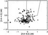 |
Fig. 2 Colour–colour diagram recommended by Stern et al. (2005) to identify AGN candidates. We compare the colour [3.6 μm − 4.5 μm] versus [5.8 μm − 8.0 μm] in AB magnitudes for our LIRGs; the area defined by the dashed lines represents the region of the colour − colour diagram populated by AGN. |
We also use the diagnostics of Brand et al. (2006) who examine the MIR slope ı of the SEDs for their sample. Here, ı corresponds to the observed flux ratio log 10(νfν(24 μm)/νfν(8 μm)). The MIR slope is supposed to be steeper for starburst-dominated sources. Brand et al. (2006) assume that sources (z > 0.6) with ı peaking at ≈ 0.0 and ≈ 0.5 are AGN- and starburst-dominated, respectively. Figure 3 shows the flux ratio ı for the total sample. For the vast majority of objects, ı is found around 0.5 ( ~17% satisfies ı ≈ 0.0), which leads us to think that starbursts dominate the MIR emission of our sample. We overplot the histogram of the objects previously identified as AGNs by Stern et al. (2005). We find that they are not necessarily identified by Brand et al. (2006).
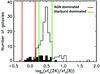 |
Fig. 3 The empty histogram illustrates the flux ratio ı = log10(νfν(24 μm)/νfν(8 μm)) for the total sample. The black histogram shows the galaxies identified as AGNs by the diagnostic of Stern et al. (2005). |
CIGALE allows estimating the fraction of Ldust due to an AGN. The code uses AGN templates from Siebenmorgen et al. (2004b,a) who provide almost 1500 AGN models differing in the luminosity of the nonthermal source, the outer radius of a spherical dust cloud covering the AGN, and the amount of attenuation in the visual caused by clouds. All models can be fed into CIGALE. Focusing on SEDs providing PAH-free MIR emission, the number of suitable models significantly decreases. As the reference model, we take L = 1012 L⊙, R = 125 pc, and AV = 32 mag (see Fig. 4). The parameter in our runs that probes the contribution of AGN radiation to Ldust is named fAGN for fraction of AGN. As input we propose values for fAGN ranging from 0.0 to 0.999. The results are presented in Sect. 4.2.
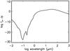 |
Fig. 4 SED of the adopted AGN template, with L = 1012 L⊙, R = 125 pc, and AV = 32 mag. |
Later we will decide to flag objects identified as AGN by at least 2 diagnostics (Stern et al. 2005; Brand et al. 2006; CIGALE).
3.4. Do we retrieve reliable parameters? Construction of a mock catalogue dedicated to the sample
The code gives an estimate of the basic input parameters, along with several additional output parameters that depend on different basic model properties. We mostly focus on SFH parameters for the young stellar population.
We performed a Bayesian analysis to estimate the physical parameters. We used a method similar to the one of Kauffmann et al. (2003a). They derive a probability distribution function (PDF) for each parameter and estimate the most probable value. We use the mean value of this distribution. The expectation value of each parameter ⟨ x ⟩ is given as 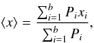 (4)and the standard deviation σ is derived by:
 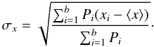 (5)This method is described as the “sum” method in Noll et al. (2009b).
When we use a numerical code based on SED-fitting, we obtain results depending on a statistical analysis. The accuracy of the estimates is directly dependent on the input fluxes (number and quality). We must check which parameter the code is able to estimate correctly. Theoretically the Bayesian analysis provides an estimation of the reliability of each parameter thanks to the shape of their PDF (if the shape is not a Gaussian curve the parameter is not correctly determined; Walcher et al. 2008), and their relative error σx.
A more straightforward approach to checking the parameter estimation is to generate a mock catalogue from the real sample. Our general strategy is to build a specific mock catalogue for each set of data (in this paper the LIRGs sample). It is made of artificial galaxies for which we not only know the flux at each wavelength, but also values of attenuation parameters and parameters of the SFH.
To construct our mock catalogue we follow 3 steps. The first step is to run the code on the data to determine the best-fitting model for each object by a simple χ2 minimization method. Each corresponds to an SED. In the second step we add an error randomly distributed according to a Gaussian curve with σ = 0.1 to each flux; it means that we add an error to the flux that is typically 10% of the flux. We have a catalogue of artificial galaxies, detected in the same filters as the observed galaxies. Then the last step is to run the code on these simulated data and to compare the exact values of the physical parameters with the values estimated by the code.
4. Results of the SED-fitting analysis
We performed SED-fitting on our LIRGs sample and on the related mock catalogue to know which parameter we are able to correctly estimate. In the following sections we describe the results of the SED-fitting of the mock catalogue with and without the band at 70 μm, and then we discuss results of the SED-fitting of the real data.
4.1. Analysis of the mock catalogue
We constructed two mock catalogues as described in Sect. 3.4 based on the 70 μm sample (sample detected at 70μm) only. The first catalogue is made of galaxies detected at 70 μm (70 μm mock sample), and the second one is made with the same galaxies for which we remove the flux at 70 μm (mock sample) in order to know if having 70 μm flux has an influence on the determination of the parameters of the SFH, or M ⋆ , Ldust and SFR.
In Fig. 5 the difference is plotted in magnitudes between the flux from the best χ2 model estimated by CIGALE and the observed flux for each broad band filter. Mean and median values are nearly equal to zero, which means that fluxes are reproduced correctly by the code to better than 0.1 mag.
Even if the code is able to reproduce the observed data correctly, we cannot settle for this result. Indeed, it is possible that some SEDs are degenerated and correspond to different parameter values. We have to compare each input parameter with its Bayesian estimation by the code. Figures 6 and 7 show the input parameters of the mock galaxies versus the values estimated by the code. Figure 6 (Fig. 7) shows results for the 70 μm mock sample (mock sample). Values of the linear Pearson correlation coefficient r are gathered in Table 3.
For the 70 μm mock sample, we find very good correlations for Mstar, SFR, Ldust, fAGN, and AV with r > 0.9. For t2, fySP, and fV, the correlation is less satisfying, because r is equal to 0.34, 0.52, and 0.64 for the 70 μm mock sample and 0.20, 0.45, and 0.64 for the mock sample. The correlation for the parameter α is good with r = 0.80 for 70 μm mock sample but very bad for the mock sample. In the following we use the mean value of α from the 70 μm sample for the objects without detection at 70 μm. For fAGN, r > 0.9 for 70 μm mock sample and 0.76 for the mock sample, with relatively small errors. Thus this parameter is correctly estimated by the code.
According to the analysis of the coefficient r and the Bayesian method’s error, the reliable parameters are Mstar, Ldust, SFR, fySP, AV, α (if 70 μm is available) and fAGN. Consequently in the next section we only study these parameters.
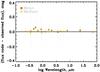 |
Fig. 5 Difference in magnitudes between the flux of the mock galaxies and the flux of the best χ2 model for these objects in each band. Red crosses and green crosses represent the mean and the median value for each wavelength. |
Estimation of the linear correlation coefficient of Pearson between the exact value and the value estimated by CIGALE for each parameter of the mock catalogue.
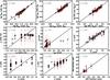 |
Fig. 6 On the x axis, the value for 8 parameters of the mock galaxies in the case of a detection at 70 μm, and on the y axis their values estimated by CIGALE. The black line corresponds to the ratio 1:1. |
4.2. Analysis of the LIRGs sample
 |
Fig. 8 Bayesian results of the code for the following parameters: Mstar, Ldust, SFR, AV, fySP, and fAGN. The empty histogram represents the total sample and the full one represents the 70 μm sample. |
We now present the results for the LIRGs sample itself. Figure 8 shows distributions for the parameters of interest, calculated with the Bayesian analysis described previously for the subsample detected at 70 μm and for the whole sample. The masses found for the 70 μm sample are shifted towards higher masses then in the total sample. We observe a similiar situation for Ldust and the SFR; the values are in the range [1011; 1012] L⊙ and [10; 92] M⊙ yr-1, respectively, with mean values higher than ones found for the total sample. This shift is expected because of the 70 μm detection limit (2.7 mJy at 5σ): at this wavelength, we only detect luminous and massive galaxies. The distribution of fySP is broad with a long tail towards high values, and AV lies between 0.5 and 2.1 mag with very few objects under 1.0 mag and quite a homogeneous distribution between 1.0 and 2.0.
Galaxies in the total sample have M ⋆ between 1010 and 1012 M⊙ with a peak at 1010.8 M⊙. We find the SFR between 3 and 92 M⊙ yr-1 with a peak at 23 M⊙ yr-1. For fySP and AV, we observe the same distribution as for the 70 μm sample. For both samples, fAGN is relatively low, between 0.0 and 0.3 with the majority of the objects in the interval [0; 0.1]. We consider that there is a definite contamination of Ldust by an AGN when fAGN > 15%, because a contamination lower than 15% does not significantly modify the total IR emission. We must also account for the uncertainty of the fAGN determination: we only consider as AGN contaminated objects with fAGN > 15% and fAGN − σAGN > 0 where σAGN is the standard deviation (see Eq. (5)).
We identify 21 objects in the total sample. The diagnostics of Stern et al. (2005) identify 31 objects and Brand et al. (2006) 9 objects. However, all the objects considered as AGN by the code are not systematically identified as AGN in the diagnostics of Brand et al. (2006) and Stern et al. (2005). We consider objects as contaminated by AGN when they are flagged by two of the three diagnostics. We identify 15 objects in the total sample of which 6 are in the 70 μm sample. These objects will be flagged in the following plots.
We have also investigated the small subsample of galaxies not detected in NUV (31 over 181 galaxies) and did not find any statistically significant difference in their main characteristics. The largest effect is found for AV: AV = 1.75+/− 0.25 mag for the non detections in NUV and AV = 1.33+/−0.34 mag for the detections in NUV. A higher dust attenuation for galaxies not detected in NUV is indeed expected.
5. Discussion
5.1. Luminosity-colour distribution and the implication for the dust temperature
SED shape of an LIRG in the 8−1000 μm range is due to emission from dust. The SED rest-frame peak defines the wavelength of maximum energetic output (in νfν). It is usually in the 40−140 μm range, and the SED is often approximated by a modified black-body (Bννβ) of T ~ 20−60 K and emissivity β ~ 1−2.
Local IRAS (Infrared Astronomical Satellite) galaxies exhibit correlations between the colour f60 μm/f100 μm and Ldust (e.g. Dale et al. 2001). The f60 μm/f100 μm ratio is often taken as an indicator of the typical heating conditions in the interstellar medium and is also indicative of a characteristic dust temperature (hereafter Tdust), f60 μm/f100 μm increasing with Tdust.
In the nearby universe, LIRGs are characterised by emission from dust at high temperatures (Sanders & Mirabel 1996). Fitting single Tdust to f60 μm/f100 μm ratio leads to Tdust ~ 20 K for low-redshift spirals (Reach et al. 1995; Dunne & Eales 2001) and 30−60 K for the high-luminosity objects typically detected by IRAS (Soifer & Neugebauer 1991; Stanford et al. 2000). High-redshift, hyperluminous galaxies can show Tdust of up to 110 K (Lewis et al. 1998).
To reproduce number counts at FIR wavelengths, Lagache et al. (2003), Chapin et al. (2009a), and Valiante et al. (2009) find that it is necessary to take cold luminous galaxies into account in the nearby universe. Cold galaxies are found to dominate the z = 0 luminosity function at low luminosities and become less important at higher redshifts, because of their passive evolution. The fraction of cold galaxies can contribute to the number counts up to 50% at 170 μm. At moderate and high redshift, the possible importance of cold, luminous galaxies has also been pointed out by Eales et al. (1999) and Chapman et al. (2002).
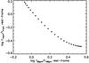 |
Fig. 9 Variations of f14 μm/f41 μm versus f60 μm/f100 μm (expressed in Jansky) for the DH02 templates used in the paper, corresponding to the α range [1.0−2.5]. |
We use the fluxes ratio f24 μm/f70 μm (corresponding to the highest wavelengths in our sample) to estimate the dust temperature. The observed f24 μm/f70 μm corresponds to f14 μm/f41 μm restframe. All our discussions are made in the framework of the DH02 models in the [1.0−2.5] α regime (see Table 2), and f14 μm/f41 μm evolves in the opposite way of f60 μm/f100 μm (i.e. Tdust, see Fig. 9).
Figure 10 exhibits the observed f24 μm/f70 μm ratio as a function of Ldust obtained for the LIRGs in the 70 μm sample. Predictions of DH02 models are overplotted. They are calibrated with the Marcillac et al. (2006) local relation between f60 μm/f100 μm (i.e. α) and Ldust. For a given Ldust we find that our galaxies have a f14 μm/f41 μm ratio higher than predicted by the models. This implies that they have a lower f60 μm/f100 μm ratio and are thus colder than expected. We cannot attribute this result to the presence of AGN contaminated objects regarding the small fraction of flagged sources.
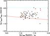 |
Fig. 10 This figure illustrates the ratio between the observed fluxes at 24 μm and 70 μm as a function of the Ldust estimated by the code. The solid red line corresponds to the results given by the DH02 templates at z = 0.7. The dashed cyan line is given by Siebenmorgen et al. (2004b) for typical AGN contaminated object. AGNs described in Sect. 4.2 are shown as red stars. |
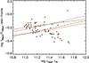 |
Fig. 11 Comparaison of the relation log 10(f60 μm/f100 μm) − log 10Ldust given by IR SEDs of DH02 after the fit to the data, with the values given by local relations and models. Upper and lower solid red lines represent local relations of Chapman et al. (2003) and Marcillac et al. (2006), respectively. We overplot models of CE01 (green dotted line), Chapin et al. (2009a) (dashed black line), and Valiante et al. (2009) (dash-dotted black line). AGN detections are shown as red stars. |
We can also directly use the f60 μm/f100 μm ratio deduced from the α parameter estimated by CIGALE. In Fig. 11 we compare Ldust and the derived f60 μm/f100 μm values of our 70 μm sample. It will make no sense to compare the rest of the sample for which we estimated α with the median value of α found for the subsample. We add to this plot the local Ldust − f60 μm/f100 μm relations of Chapman et al. (2003) and Marcillac et al. (2006), and the luminosity-temperature models proposed by CE01, Chapin et al. (2009a), and Valiante et al. (2009) in the luminosity range [1011; 1012] L⊙. Figure 11 shows that the code gives a different trend for the relation f60 μm/f100 μm versus Ldust than both local relations and models. Galaxies having the lowest IR luminosity agree with them, but more luminous objects are found to be colder than predicted, and globally they evolve in the opposite way to local relations and models. Chanial et al. (2007) make a selection at 60 and 170 μm respectively using IRAS and ISO observations at z = 0 and find that galaxies selected at 170 μm are colder than ones detected at shorter wavelengths. They conclude that selecting galaxies at long wavelengths introduce a bias towards cold galaxies. Selecting the sample at a wavelength longwards of the peak, by definition, does not lead to warm sources (Sanders & Mirabel 1996). Our sample is selected by restframe ~41 μm emission, i.e., on warm dust; yet, we mostly find colder Tdust at a given luminosity than predicted by models of DH02 and CE01, calibrated in the nearby universe. This tends to support the interpretation that the offset found towards colder temperatures at a given luminosity is at least in part a real difference. Zheng et al. (2007) suggest that this tendency towards colder Tdust reflects a difference in dust and star formation geometry. Although local LIRGs tend to be interacting systems with relatively compact very intense star formation and of comparable masses (e.g., Wang et al. 2006), 0.5 < z < 1 LIRGs tend to be disk-dominated, relatively undisturbed galaxies (Zheng et al. 2004; Bell et al. 2005; Melbourne et al. 2005). They suggest that these diskgalaxies host widespread, intense star formation, much like star formation in local spirals but scaled up, leading to relatively cold Tdust.
Our results agree with Symeonidis et al. (2009). They compare FIR properties of LIRGs and Ultra Luminous InfraRed Galaxies (ULIRGs, Ldust > 1012 L⊙) in the 0.1 < z < 2 redshift range, based on MIPS and IRAC data with Ldust > 1010 L⊙, 70 μm selected objects, with those of local sources of equivalent luminosity from the local IRAS Bright Galaxy Sample. They fit their data with the Siebenmorgen & Krügel (2007) theoretical SED templates and find that their distant LIRGs and ULIRGs are colder than their local equivalents. They find a significant cold-dust associated FIR excess not detected in local sources of comparable luminosity directly linked to the evolution in dust and star formation properties from the local to the high-redshift Universe.
Herschel is now providing longward 70 μm data allowing a reliable estimation of Tdust.
5.2. Star formation rate and stellar mass
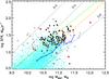 |
Fig. 12 The relation SFR − M ⋆ for the total sample. Filled circles (empty circles) illustrate galaxies for which the age of the young stellar population is found to be greater (lower than or equal to) than 0.3 Gyr by CIGALE. AGNs are represented by red stars. We overplot the semi-analytical Millennium simulations (cyan diamonds), analytical models of Buat et al. (2008) (dash-dotted yellow line) at z = 0.7 and Noeske et al. (2007a) (connected blue crosses) at z ~ 0.7 with observations of Elbaz et al. (2007) (solid black line, z = 0 and 1), Daddi et al. (2007) (solid black line z = 2), and Santini et al. (2009) at z ~ 0.7 (dashed green line). |
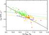 |
Fig. 13 The SSFR − M ⋆ relation for the total sample. Green dots and yellow dots represent objects for which fySP are larger or lower than 10%, respectively. AGN contaminated objects are represented by red stars. The black dashed line shows the detection limit. We overplot analytical models of Buat et al. (2008) (dash-dotted yellow line) at z = 0.7 and Noeske et al. (2007a) (connected blue crosses) at z ~ 0.7, and observations of Elbaz et al. (2007) (solid black line, z = 1) and Santini et al. (2009) at z ~ 0.7 (dashed green line). |
How and when galaxies build up their M ⋆ is still a major question in observational cosmology. While a general consensus has been reached in recent years on the evolution of the galaxy stellar mass function (e.g., Dickinson et al. 2003; Drory et al. 2004; Bundy et al. 2005; Pannella 2006; Marchesini et al. 2009), the redshift evolution of the SFR as a function of M ⋆ still remains unclear. The evolution of the galaxy SFR − M ⋆ relationship provides key constraints on M ⋆ assembly histories of galaxies. For star-forming galaxies a correlation is observed between SFR and M ⋆ with a slope near to unity from z ~ 0 to 2 and a scatter of 0.3 dex (Daddi et al. 2007; Elbaz et al. 2007; Noeske et al. 2007a). The slope and scatter are expected to be a direct reflection of the similarity in the shape of galaxy SFHs among various models and at various masses (Davé 2008; Noeske et al. 2007b). It is worth noting that other z = 2 observations suggest a somewhat large scatter (Shapley et al. 2005; Papovich et al. 2006), so the observational picture is not entirely settled.
Figure 12 shows the SFR of each galaxy of our sample as a function of the corresponding M ⋆ and the results of various models and observations: analytical models of Buat et al. (2008) and Noeske et al. (2007a), the semi-analytical Millennium simulations of Kitzbichler & White (2007) used in Buat et al. (2008) and observations of Elbaz et al. (2007), Daddi et al. (2007), and Santini et al. (2009). Our sample of LIRGs has an average redshift of ~ 0.7. We find the vast majority of the sample between the correlations at z = 0 and z = 1 given by Elbaz et al. (2007). Our data cover the extreme part of the Millennium simulations where we can find galaxies with the largest SFRs between ~ 10−100 M⊙ yr-1. We do not observe a correlation between SFR and M ⋆ , but instead a flat distribution of SFR. We consider a tight range of SFR since we select objects with Ldust  1011 L⊙ (see below). This range is not sufficient to search for a general correlation between M ⋆ and the SFR; however, we observe a large scatter in M ⋆ in the considered SFR range. Indeed galaxies whose young stellar population is younger than 300 Myr exhibit a larger dispersion in M ⋆ than galaxies whose SFR is constant over a longer period (Fig. 12), therefore the SFH of our objects has an influence on the dispersion of the SFR − M ⋆ plot. This agrees with the conclusions of Davé (2008) and Noeske et al. (2007b).
The specific star formation rate (SSFR) defined as the ratio between SFR and M ⋆ (e.g., Kennicutt et al. 2005) is also commonly used to trace the SFH in galaxies. The SSFR is plotted in Fig. 13 as a function of the corresponding M ⋆ , and we can see the increase in the SSFRs towards lower M ⋆ . Before any interpretation we can estimate a detection limit in SSFR: Ldust = 1011 L⊙ translates into SFRlim = 17.78 M⊙ yr-1 at z = 0.7 (Eq. (1) of Buat et al. 2008). We overlay this detection limit and see that the trend of SSFR with M ⋆ is largely constrained by this limit. We compare our results with the same models and observations as illustrated in Fig. 12. SSFRs of our intermediate-mass galaxies (M ⋆ ≤ 1011 M⊙) agree with those observed by Santini et al. (2009), but for these values of M ⋆ we cannot detect more quiescent galaxies because of the detection limit. SSFRs of high-mass galaxies (M ⋆ > 1011 M⊙) are better described by the models of Buat et al. (2008). These massive galaxies have SSFRs which do not exceed 2.5 × 10⁻¹⁰ yr-1 (corresponding to a SFR ~ 25 M⊙ yr-1) and never reach the SSFRs of intermediate-mass galaxies observed in this study. To distinguish galaxies for which the young stellar population significantly contributes to M ⋆ , we identify objects for which fySP estimated with CIGALE is larger or lower than 10% and see that the 2 groups are separated well according to their stellar mass. Galaxies with M ⋆ ≤ 1011 M⊙ have more than 10% of their mass due to the young stellar population, whereas in galaxies with M ⋆ > 1011 M⊙ this mass represents less than 10%. This result agrees with the common picture that massive galaxies formed the bulk of their stars early and on shorter time scales, while numerous less massive galaxies evolve on longer time scales, a phenomenon generally linked to the downsizing scenario (e.g. Cowie et al. 1996; Brinchmann & Ellis 2000; Fontana et al. 2003; Feulner et al. 2005; Pérez-González et al. 2005; Papovich et al. 2006; Damen et al. 2009).
6. Conclusions
We performed an SED-fitting analysis of a sample of LIRGs at z = 0.7 detected at 24 μm by Spitzer/MIPS, for which 80% of the objects have a detection at 231 nm by GALEX. This sample is observed over a wide range of wavelengths from NUV to FIR (70 μm) and is made of 181 galaxies with 62 detected at 70 μm. We fit the SEDs of our galaxies with the CIGALE code (Burgarella et al. 2005; Noll et al. 2009b), which combines stellar and dust emissions in a physical way. This study is the first use of CIGALE at a redshift higher than 0. The stellar populations synthesis code of Maraston et al. (2005) is adopted to model the stellar emission (UV, optical, and NIR wavelengths). Then the code uses semi-empirical one-parameter models of Dale & Helou (2002) to reproduce the dust emission in MIR-to-FIR wavelengths.
CIGALE allows estimation of several physical parameters based on a Bayesian-like analysis. We show that we are able to estimate reliable stellar masses, SFRs, fractions of young stellar population, Dale & Helou (2002) IR-templates parameter α (if 70 μm is available), dust attenuation, dust luminosities, as well as the fraction of dust emission from an AGN. The investigation is performed by building mock catalogues based on the real samples.
The 70 μm sample exhibits colder dust temperatures (as traced by the ratio L24 μm/L70 μm and the α parameter of the Dale & Helou 2002 templates) than expected from local relations between dust luminosity and temperature, confirming other recent results for similar samples. Our LIRGs appear to form stars actively. They exhibit a flat distribution with a large scatter in the SFR – stellar mass plot. The amplitude of the dispersion is related to the age of the young stellar population, with a tighter distribution found for the oldest ages. We find that our galaxies with a stellar mass >1011 M⊙ have less than 10% of their mass coming from the young stellar population. The SSFR for these massive galaxies never reaches the one found for intermediate-mass galaxies of our sample, confirming the downsizing scenario.
The multiwavelength data analysis performed in this study provides reliable estimates of several physical parameters, but may turn out insufficient for determining accurate dust temperatures. Forthcoming data from Herschel will help us to better constrain galaxies SEDs and thus to derive more reliable parameters.
Web address to use CIGALE: http://www.oamp.fr/cigale/
MUSYC collaboration: http://www.astro.yale.edu/MUSYC/
References
- Arnouts, S., Vandame, B., Benoist, C., et al. 2001, A&A, 379, 740 [NASA ADS] [CrossRef] [EDP Sciences] [Google Scholar]
- Arnouts, S., Schiminovich, D., Ilbert, O., et al. 2005, ApJ, 619, L43 [NASA ADS] [CrossRef] [Google Scholar]
- Arnouts, S., Walcher, C. J., Le Fèvre, O., et al. 2007, A&A, 476, 137 [NASA ADS] [CrossRef] [EDP Sciences] [Google Scholar]
- Basu-Zych, A. R., Schiminovich, D., Johnson, B., et al. 2007, ApJS, 173, 457 [NASA ADS] [CrossRef] [Google Scholar]
- Bauer, F. E., Alexandern, D. M., Brandt, W. N., et al. 2004, AJ, 128, 2048 [NASA ADS] [CrossRef] [Google Scholar]
- Bell, E. F., MacIntosh, D. H., Katz, N., & Weinberg, N. D. 2003, ApJS, 149, 289 [NASA ADS] [CrossRef] [Google Scholar]
- Bell, E. F., Papovich, C., Wolf, C., et al. 2005, ApJ, 625, 36 [Google Scholar]
- Bell, E. F., Zheng, X. Z., Papovich, C., et al. 2007, ApJ, 663, 834 [NASA ADS] [CrossRef] [Google Scholar]
- Brand, K., Weedman, D., Desai, V., et al. 2006, ApJ, 644, 147 [Google Scholar]
- Brinchmann, J., & Ellis, R. S. 2000, ApJ, 536, 77 [Google Scholar]
- Brinchmann, J., Charlot, S., White, S. D. M., et al. 2004, MNRAS, 351, 1151 [NASA ADS] [CrossRef] [Google Scholar]
- Bruzual, G., & Charlot, S. 2003, MNRAS, 344, 1000 [NASA ADS] [CrossRef] [Google Scholar]
- Buat, V., Deharveng, J. M., Burgarella, D., & Kunth, D. 2002, A&A, 393, 33 [NASA ADS] [CrossRef] [EDP Sciences] [Google Scholar]
- Buat, V., Iglesias-Páramo, J., Seibert, M., et al. 2005, ApJ, 619, L51 [NASA ADS] [CrossRef] [Google Scholar]
- Buat, V., Takeuchi, T. T., Iglesias-Páramo, J., et al. 2007a, ApJS, 173, 404 [NASA ADS] [CrossRef] [Google Scholar]
- Buat, V., Marcillac, D., Burgarella, D., et al. 2007b, A&A, 469, 19 [Google Scholar]
- Buat, V., Boissier, S., Burgarella, D., et al. 2008, A&A, 483, 107 [NASA ADS] [CrossRef] [EDP Sciences] [Google Scholar]
- Bundy, K., Ellis, R. S., & Conselice, C. J. 2005, ApJ, 625, 621 [NASA ADS] [CrossRef] [Google Scholar]
- Burgarella, D., Buat, V., & Iglesias-Páramo, J. 2005, MNRAS, 1413, 1425 [Google Scholar]
- Burgarella, D., Pérez-González, P., Tyler, K. D., et al. 2006, A&A, 450, 69 [NASA ADS] [CrossRef] [EDP Sciences] [Google Scholar]
- Burgarella, D., Le Floc’h, E.,Takeuchi, T. T., et al. 2007, MNRAS, 380, 986 [NASA ADS] [CrossRef] [Google Scholar]
- Caputi, K. I., Lagache, G., Yan, L., et al. 2007, ApJ, 660, 97 [NASA ADS] [CrossRef] [Google Scholar]
- Chanial, P., Flores, H., Guiderdoni, B., et al. 2007, 462, 81 [Google Scholar]
- Calzetti, D., Armus, L., Bohlin, R. C., et al. 2000, 533, 682 [Google Scholar]
- Chapin, E. L., Hugues, D. H., Aretxaga, I., et al. 2009, MNRAS, 393, 653 [NASA ADS] [CrossRef] [Google Scholar]
- Chary, R. R., & Elbaz, D. 2001, ApJ, 556, 562 [NASA ADS] [CrossRef] [Google Scholar]
- Chapman, S. C., Smail, I., Ivison, R. J., et al. 2002, ApJ, 573, 66 [NASA ADS] [CrossRef] [Google Scholar]
- Chapman, S. C., Helou, G., Lewis, G. F., & Dale, D. A. 2003, ApJ, 588, 186 [NASA ADS] [CrossRef] [Google Scholar]
- Conroy, C. 2009, ApJ, 647, 201 [Google Scholar]
- Conroy, C., Gunn, J. E., & White, M. 2009, ApJ, 699, 486 [NASA ADS] [CrossRef] [Google Scholar]
- Cowie, L. L., & Barger, A. J. 2008, ApJ, 686, 72 [NASA ADS] [CrossRef] [Google Scholar]
- Cowie, L. L., Songaila, A., Hu, E. M., & Cohen, J. G. 1996, AJ, 112, 839 [Google Scholar]
- Daddi, E., Dickinson, M., Morrison, G., et al. 2007, ApJ, 670, 172 [NASA ADS] [CrossRef] [Google Scholar]
- Dale, D., & Helou, G. 2002, ApJ, 576, 159 [NASA ADS] [CrossRef] [Google Scholar]
- Dale, D. A., Helou, G., Contursi, A., Silbermann, N. A., & Kolhatkar, S. 2001, ApJ, 549, 215 [NASA ADS] [CrossRef] [Google Scholar]
- Damen, M., Labbé, I., Franx, M., et al. 2009, ApJ, 690, 937 [NASA ADS] [CrossRef] [Google Scholar]
- da Cunha, E., Charlot, S., & Elbaz, D. 2008, MNRAS, 388, 1595 [NASA ADS] [CrossRef] [Google Scholar]
- Davé, R. 2008, MNRAS, 385, 147 [NASA ADS] [CrossRef] [Google Scholar]
- Dickinson, M., Papovich, C., Ferguson, H. C., & Budavári, T. 2003, ApJ, 587, 25 [NASA ADS] [CrossRef] [Google Scholar]
- Drory, N., Bender, R., Feulner, G., et al. 2004, ApJ, 608, 742 [NASA ADS] [CrossRef] [Google Scholar]
- Dunne, L., & Eales, S. A. 2001, MNRAS, 327, 697 [NASA ADS] [CrossRef] [Google Scholar]
- Dopita, M. A., Groves, B. A., Fischera, J., et al. 2005, ApJ, 619, 755 [NASA ADS] [CrossRef] [Google Scholar]
- Dye, S. 2008, MNRAS, 328, 1293 [NASA ADS] [CrossRef] [Google Scholar]
- Eales, S., Lilly, S., Gear, W., et al. 1999, ApJ, 515, 518 [NASA ADS] [CrossRef] [Google Scholar]
- Elbaz, D., Daddi, E., Le Borgne, D., et al. 2007, A&A, 468, 33 [NASA ADS] [CrossRef] [EDP Sciences] [Google Scholar]
- Erb, D. K., Steidel, C. C., Shapley, A. E., et al. 2006, ApJ, 646, 107 [NASA ADS] [CrossRef] [Google Scholar]
- Fadda, D., Flores, H., Hasinger, G., et al. 2002, A&A, 383, 838 [NASA ADS] [CrossRef] [EDP Sciences] [Google Scholar]
- Fazio, G. G., Hora, J. L., Allen, L. E., et al. 2004, ApJS, 154, 10 [NASA ADS] [CrossRef] [Google Scholar]
- Feulner, G., Goronova, Y., Drory, N., Hopp, U., & Bender, R. 2005, MNRAS, 358, L1 [NASA ADS] [CrossRef] [Google Scholar]
- Fioc, M., & Rocca-Volmerange, B. 1997, A&A, 326, 950 [NASA ADS] [Google Scholar]
- Franceschini, A., Manners, J., Polletta, M. C., et al. 2005, AJ, 129, 2074 [NASA ADS] [CrossRef] [Google Scholar]
- Fontana, A., Donnarumma, I., Vanzella, E., et al. 2003, ApJ, 594, 9 [Google Scholar]
- Genzel, R., Lutz, D., Sturm, E., et al. 1998, ApJ, 498, 579 [NASA ADS] [CrossRef] [Google Scholar]
- Giacconi, R., Zirm, A., Wang, J. X., et al. 2002, ApJS, 139, 369 [NASA ADS] [CrossRef] [Google Scholar]
- Gruppioni, C., Pozzi, F., Polletta, M., et al. 2008, ApJ, 684, 136 [NASA ADS] [CrossRef] [Google Scholar]
- Iglesias-Páramo, J., Buat, V., Hernández-Fernández, J., et al. 2007, ApJ, 670, 279 [NASA ADS] [CrossRef] [Google Scholar]
- Ishida, C. M. 2004, Thesis (Ph.D.), University of HAWAI’I, Source DAI-B 65/04, Oct., 1908, 502 [Google Scholar]
- Kauffmann, G., Heckman, T. M., White, S. D. M., et al. 2003, MNRAS, 341, 33 [NASA ADS] [CrossRef] [Google Scholar]
- Kaviraj, S., Khochfar, S., Schawinski, K., et al. 2009, MNRAS, 394, 67 [NASA ADS] [CrossRef] [Google Scholar]
- Kennicutt, R. C. 1998, ApJ, 498, 541 [NASA ADS] [CrossRef] [Google Scholar]
- Kennicutt, R. C., Jr., Lee, J. C., Funes, J. G., Sakai, S., & Akiyama, S. 2005, in Starbursts: From 30 Doradus to Lyman Break Galaxies, ed. R. de Grijs, & R. M. González Delgado (Dordrecht: Springer), ASSL, 329, 187 [Google Scholar]
- Kitzbichler, M. G., & White, S. D. M. 2007, MNRAS, 376, 2 [NASA ADS] [CrossRef] [Google Scholar]
- Lagache, G., Dole, H., & Pujet, J.-L. 2003, MNRAS, 338, 555 [NASA ADS] [CrossRef] [Google Scholar]
- Lagache, G., Dole, H., Pujet, J.-L., et al. 2004, ApJ, 154, 112 [Google Scholar]
- Lee, S.-K., Idzi, R., Ferguson, H. C., et al. 2009, ApJ, 184, 100 [NASA ADS] [Google Scholar]
- Le Borgne, D., Elbaz, D., Ocvirk, P., & Pichon, C. 2009, A&A, 504, 727 [NASA ADS] [CrossRef] [EDP Sciences] [Google Scholar]
- Le Floc’h, E.,Papovich, C., Dole, H., et al. 2005, ApJ, 632, 169 [NASA ADS] [CrossRef] [Google Scholar]
- Lewis, G. F., Chapman, S. C., Ibata, R. A., et al. 1998, ApJ, 505, L1 [NASA ADS] [CrossRef] [Google Scholar]
- Magnelli, B., Elbaz, D., Chary, R. R., et al. 2009, A&A, 496, 57 [NASA ADS] [CrossRef] [EDP Sciences] [Google Scholar]
- Manners, J. C., Serjeant, S., Bottinelli, S., et al. 2004, MNRAS, 355, 97 [NASA ADS] [CrossRef] [Google Scholar]
- Maraston, C. 1998, MNRAS, 300, 872 [NASA ADS] [CrossRef] [Google Scholar]
- Maraston, C. 2005, MNRAS, 362, 799 [NASA ADS] [CrossRef] [Google Scholar]
- Maraston, C., Daddi, E., Renzini, A., et al. 2006, ApJ, 652, 85 [NASA ADS] [CrossRef] [Google Scholar]
- Marchesini, D., van Dokkum, P. G., Förster Schreiber, N. M., et al. 2009, ApJ, 701, 1765 [NASA ADS] [CrossRef] [Google Scholar]
- Marcillac, D., Elbaz, D., Chary, R. R., et al. 2006, A&A, 451, 57 [NASA ADS] [CrossRef] [EDP Sciences] [Google Scholar]
- Martin, C., Small, T., Schiminovich, D., et al. 2007, ApJS, 173, 415 [NASA ADS] [CrossRef] [Google Scholar]
- Melbourne, J., Koo, D. C., & Le Floc’h, E. 2005, ApJ, 632, L65 [NASA ADS] [CrossRef] [Google Scholar]
- Noeske, K. G., Weiner, B. J., Faber, S. M., et al. 2007a, ApJ, 660, L43 [Google Scholar]
- Noeske, K. G., Weiner, B. J., Faber, S. M., et al. 2007b, ApJ, 660, L47 [NASA ADS] [CrossRef] [Google Scholar]
- Noll, S., Pierini, D., Cimatti, E., et al. 2009a, A&A, 499, 69 [NASA ADS] [CrossRef] [EDP Sciences] [Google Scholar]
- Noll, S., Burgarella, D.,Giovannoli, E., et al. 2009b, A&A, 507, 1793 [NASA ADS] [CrossRef] [EDP Sciences] [Google Scholar]
- Pannella, M., Hopp, U., Saglia, R. P., et al. 2006, ApJ, 639, 1 [Google Scholar]
- Pannella, M., Carilli, C. D., Daddi, E., et al. 2009, ApJ, 698, L116 [Google Scholar]
- Panuzzo, P., Silva, L., Granato, G. L., et al. 2005, AIP Conf. Proc., 761, 187 [NASA ADS] [CrossRef] [Google Scholar]
- Papovich, C., Dole, H., Egami, E., et al. 2004, ApJS, 154, 70 [NASA ADS] [CrossRef] [Google Scholar]
- Papovich, C., Moustakas, L. A., Dickinson, M., et al. 2006, ApJ, 640, 92 [NASA ADS] [CrossRef] [Google Scholar]
- Pérez-González, P. G., Rieke, G. H., Egami, E., et al. 2005, ApJ, 630, 82 [NASA ADS] [CrossRef] [Google Scholar]
- Reach, W. T., Dweck, E., Fixsen, D. J., et al. 1995, ApJ, 451, 188 [NASA ADS] [CrossRef] [Google Scholar]
- Renzini, A. 2009, MNRAS, 398, L58 [NASA ADS] [Google Scholar]
- Rieke, G. H., Young, E. T., Engelbracht, C. W., et al. 2004, ApJS, 154, 25 [NASA ADS] [CrossRef] [Google Scholar]
- Rieke, G. H., Alonso-Herrero, A., Weiner, B. J., et al. 2009, ApJ, 692, 556 [NASA ADS] [CrossRef] [Google Scholar]
- Salim, S., Charlot, S., Rich, R. M., et al. 2005, ApJ, 619, L39 [Google Scholar]
- Salim, S., Rich, R., Charlot, S., et al. 2007, ApJS, 173, 267 [NASA ADS] [CrossRef] [Google Scholar]
- Salim, S., Dickinson, M., Rich, R. M., et al. 2009, ApJ, 700, 161 [NASA ADS] [CrossRef] [MathSciNet] [Google Scholar]
- Salimbeni, S., Fontana, A., Giallongo, E., et al. 2009, AIPC, 1111, 207 [Google Scholar]
- Sanders, D. B., & Mirabel, I. F. 1996, A&A, 34, 749 [CrossRef] [Google Scholar]
- Santini, P., Fontana, A., Grazian, A., et al. 2009, A&A, 504, 751 [NASA ADS] [CrossRef] [EDP Sciences] [Google Scholar]
- Seymour, N., Symeonidis, M., Page, M. J., et al. 2009, MNRAS, 398, 1573 [Google Scholar]
- Shapley, A. E., Steidel, C. C., Erb, D. K., et al. 2005, ApJ, 626, 698 [NASA ADS] [CrossRef] [Google Scholar]
- Siebenmorgen, R., & Krügel, E. 2007, A&A, 461, 445 [NASA ADS] [CrossRef] [EDP Sciences] [Google Scholar]
- Siebenmorgen, R., Freudling, W., Krügel, E., & Haas, M. 2004a, A&A, 421, 129 [NASA ADS] [CrossRef] [EDP Sciences] [Google Scholar]
- Siebenmorgen, R., Krügel, E., & Spoon, H. W. W. 2004b, A&A, 414, 123 [NASA ADS] [CrossRef] [EDP Sciences] [Google Scholar]
- Silva, L., Granato, G. L., Bressan, A., & Danese, L. 1998, ApJ, 509, 103 [NASA ADS] [CrossRef] [Google Scholar]
- Silva, L., Maiolino, R., & Granato, G. L. 2004, MNRAS, 355, 973 [NASA ADS] [CrossRef] [Google Scholar]
- Soifer, B. T., & Neugebauer, G. 1991, AJ, 101, 354 [NASA ADS] [CrossRef] [Google Scholar]
- Stanford, S. A., Stern, D., Van Breugel, W., & De Breuk, C. 2000, ApJS, 131, 185 [NASA ADS] [CrossRef] [Google Scholar]
- Stern, D., Eisenhardt, P., Gorjian, V., et al. 2005, ApJ, 631, 163 [NASA ADS] [CrossRef] [Google Scholar]
- Symeonidis, M., Page, M. J., Seymour, N., et al. 2009, MNRAS, 397, 1728 [NASA ADS] [CrossRef] [Google Scholar]
- Taylor, E. N., Franx, M., van Dokkum, P. G., & Quadri, R. F. 2009, ApJS, 183, 295 [NASA ADS] [CrossRef] [Google Scholar]
- Tonini, C., Maraston, C., Devriendt, J., Thomas, D., & Silk, J. 2009, MNRAS, 396, 36 [Google Scholar]
- Valiante, E., Lutz, D., Sturm, E., Genzel, R., & Chapin, E. L. 2009, ApJ, 701, 1814 [NASA ADS] [CrossRef] [Google Scholar]
- Walcher, C. J., Lamareille, F., Arnouts, S., et al. 2008, A&A, 491, 713 [NASA ADS] [CrossRef] [EDP Sciences] [Google Scholar]
- Wang, J. L., Xia, X. Y., Mao, S., et al. 2006, ApJ, 649, 722 [NASA ADS] [CrossRef] [Google Scholar]
- Werner, M. W., Roellig, T. L., Low, F. J., et al. 2004, ApJS, 154, 1 [Google Scholar]
- Wolf, C., Meisenheimer, K., Kleinheinrich, M., et al. 2004, A&A, 421, 913 [NASA ADS] [CrossRef] [EDP Sciences] [Google Scholar]
- Wuyts, S., Franx, M., Cox, T. J., et al. 2009, ApJ, 696, 348 [NASA ADS] [CrossRef] [Google Scholar]
- Zheng, X. Z., Hammer, F., Flores, H., Assémat, F., & Pelat, D. 2004, A&A, 421, 847 [NASA ADS] [CrossRef] [EDP Sciences] [Google Scholar]
- Zheng, X. Z., Dole, H., Bell, E. F., et al. 2007, ApJ, 670, 301 [NASA ADS] [CrossRef] [Google Scholar]
All Tables
The observed data: wavelengths corresponding to the filters’ identification of instrument and survey.
List of the input parameters of the code CIGALE and their selected range for a specific run.
Estimation of the linear correlation coefficient of Pearson between the exact value and the value estimated by CIGALE for each parameter of the mock catalogue.
All Figures
|
Fig. 1 Scenario of SFH: two bursts, one for the old stellar population having a moderate e-folding time and one for the young stellar population constant over time. |
| In the text | |
|
Fig. 2 Colour–colour diagram recommended by Stern et al. (2005) to identify AGN candidates. We compare the colour [3.6 μm − 4.5 μm] versus [5.8 μm − 8.0 μm] in AB magnitudes for our LIRGs; the area defined by the dashed lines represents the region of the colour − colour diagram populated by AGN. |
| In the text | |
|
Fig. 3 The empty histogram illustrates the flux ratio ı = log10(νfν(24 μm)/νfν(8 μm)) for the total sample. The black histogram shows the galaxies identified as AGNs by the diagnostic of Stern et al. (2005). |
| In the text | |
|
Fig. 4 SED of the adopted AGN template, with L = 1012 L⊙, R = 125 pc, and AV = 32 mag. |
| In the text | |
|
Fig. 5 Difference in magnitudes between the flux of the mock galaxies and the flux of the best χ2 model for these objects in each band. Red crosses and green crosses represent the mean and the median value for each wavelength. |
| In the text | |
|
Fig. 6 On the x axis, the value for 8 parameters of the mock galaxies in the case of a detection at 70 μm, and on the y axis their values estimated by CIGALE. The black line corresponds to the ratio 1:1. |
| In the text | |
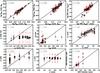 |
Fig. 7 Same plot as Fig. 6 in the case of non-detection at 70 μm. |
| In the text | |
|
Fig. 8 Bayesian results of the code for the following parameters: Mstar, Ldust, SFR, AV, fySP, and fAGN. The empty histogram represents the total sample and the full one represents the 70 μm sample. |
| In the text | |
|
Fig. 9 Variations of f14 μm/f41 μm versus f60 μm/f100 μm (expressed in Jansky) for the DH02 templates used in the paper, corresponding to the α range [1.0−2.5]. |
| In the text | |
|
Fig. 10 This figure illustrates the ratio between the observed fluxes at 24 μm and 70 μm as a function of the Ldust estimated by the code. The solid red line corresponds to the results given by the DH02 templates at z = 0.7. The dashed cyan line is given by Siebenmorgen et al. (2004b) for typical AGN contaminated object. AGNs described in Sect. 4.2 are shown as red stars. |
| In the text | |
|
Fig. 11 Comparaison of the relation log 10(f60 μm/f100 μm) − log 10Ldust given by IR SEDs of DH02 after the fit to the data, with the values given by local relations and models. Upper and lower solid red lines represent local relations of Chapman et al. (2003) and Marcillac et al. (2006), respectively. We overplot models of CE01 (green dotted line), Chapin et al. (2009a) (dashed black line), and Valiante et al. (2009) (dash-dotted black line). AGN detections are shown as red stars. |
| In the text | |
|
Fig. 12 The relation SFR − M ⋆ for the total sample. Filled circles (empty circles) illustrate galaxies for which the age of the young stellar population is found to be greater (lower than or equal to) than 0.3 Gyr by CIGALE. AGNs are represented by red stars. We overplot the semi-analytical Millennium simulations (cyan diamonds), analytical models of Buat et al. (2008) (dash-dotted yellow line) at z = 0.7 and Noeske et al. (2007a) (connected blue crosses) at z ~ 0.7 with observations of Elbaz et al. (2007) (solid black line, z = 0 and 1), Daddi et al. (2007) (solid black line z = 2), and Santini et al. (2009) at z ~ 0.7 (dashed green line). |
| In the text | |
|
Fig. 13 The SSFR − M ⋆ relation for the total sample. Green dots and yellow dots represent objects for which fySP are larger or lower than 10%, respectively. AGN contaminated objects are represented by red stars. The black dashed line shows the detection limit. We overplot analytical models of Buat et al. (2008) (dash-dotted yellow line) at z = 0.7 and Noeske et al. (2007a) (connected blue crosses) at z ~ 0.7, and observations of Elbaz et al. (2007) (solid black line, z = 1) and Santini et al. (2009) at z ~ 0.7 (dashed green line). |
| In the text | |
Current usage metrics show cumulative count of Article Views (full-text article views including HTML views, PDF and ePub downloads, according to the available data) and Abstracts Views on Vision4Press platform.
Data correspond to usage on the plateform after 2015. The current usage metrics is available 48-96 hours after online publication and is updated daily on week days.
Initial download of the metrics may take a while.