| Issue |
A&A
Volume 524, December 2010
|
|
|---|---|---|
| Article Number | A91 | |
| Number of page(s) | 16 | |
| Section | Interstellar and circumstellar matter | |
| DOI | https://doi.org/10.1051/0004-6361/201015143 | |
| Published online | 25 November 2010 | |
Physical properties of dense cores in Orion B9⋆
1
Finnish Centre for Astronomy with ESO (FINCA), University of
Turku
Väisäläntie 20
21500
Piikkiö
Finland
e-mail: oskari.miettinen@helsinki.fi
2 Department of Physics, PO Box 64, 00014 University of
Helsinki, Finland
Received:
3
June
2010
Accepted:
7
September
2010
Aims. We aim to determine the physical and chemical properties of the starless and protostellar cores in Orion B9, which represents a relatively quiescent star-forming region in Orion B.
Methods. We observed the NH3 (J,K) = (1,1) and (2,2) inversion lines and the N2H+(3−2) rotational lines, with the Effelsberg 100-m and APEX telescopes, respectively, towards the submillimetre peak positions in Orion B9. These data are used in conjunction with our APEX/LABOCA 870 μm dust continuum data of the region.
Results. The gas kinetic temperature in the cores derived from the NH3 data is between ~9.4−13.9 K. The non-thermal velocity dispersion is subsonic in most of the cores. The non-thermal linewidth in protostellar cores appears to increase with increasing bolometric luminosity. The core masses, ~2−8 M⊙, are very likely drawn from the same parent distribution as the core masses in Orion B North. Based on the virial parameter analysis, starless cores in the region are likely to be gravitationally bound, and thus prestellar. Some of the cores have a lower radial velocity than the systemic velocity of the region, suggesting that they are members of the “low-velocity part” of Orion B. The observed core-separation distances deviate from the corresponding random-like model distributions. The distances between the nearest neighbours are comparable to the thermal Jeans length. The fractional abundances of NH3 and N2H+ in the cores are ~1.5−9.8 × 10⁻⁸ and ~0.2−5.9 × 10⁻¹⁰, respectively. The NH3 abundance appears to decrease with increasing H2 column and number densities. The NH3/N2H+ column density ratio is larger in starless cores than in cores with embedded protostars.
Conclusions. The core population in Orion B9 is comparable in physical properties to those in nearby low-mass star-forming regions. The Orion B9 cores also seem to resemble cores found in isolation rather than those associated with clusters. Moreover, because the cores may not be randomly distributed within the region (contrary to what was suggested in our Paper I), it is unclear whether the origin of cores could be explained by turbulent fragmentation. On the other hand, many of the core properties conform to the picture of dynamic core evolution. The Orion B9 region has probably been influenced by the feedback from the nearby Ori OB 1b group, and the fragmentation of the parental cloud into cores could be caused by gravitational instability.
Key words: stars: formation / ISM: clouds / ISM: individual objects: Orion B / ISM: molecules / radio lines: ISM
This publication is based on data acquired with the Atacama Pathfinder Experiment (APEX) under programme 084.F-9312, and observations with the 100-m telescope of the Max-Planck-Institut für Radioastronomie (MPIfR) at Effelsberg. APEX is a collaboration between the MPIfR, the European Southern Observatory, and the Onsala Space Observatory.
© ESO, 2010
1. Introduction
The Orion B molecular cloud (L1630) is a useful target for studying dense cores and the
processes of star formation. The cloud complex lies at a relatively close distance to the
Sun (~450 pc), and it contains a wide range of star-forming environments, such as the
high-mass star-forming region NGC 2024 and several other regions of clustered star formation
(which is the dominant mode of star formation in the Galaxy), but also more quiescent areas
(see, e.g., Bally 2008; Ikeda et al. 2009; Buckle et al.
2010). We recently mapped region of the central part of Orion B of about 36′ × 27′
(4.7 pc × 3.5 pc), called Orion B9 ( ,
,  ), at 870 μm dust continuum using
LABOCA on APEX, and discovered 12 dense submm cores (Miettinen et al. 2009; hereafter Paper I). The cores were classified into starless
and protostellar ones by using the Spitzer data, yielding the result that half the cores
have embedded protostar(s). In the present paper, we examine the physical characteristics of
the Orion B9 cores further. To determine the gas kinetic temperature, kinematics, and the
dynamical state of the cores, we performed NH3(1,1) and
(2,2), and N2H+(3−2) observations towards the
core submm peak positions with the Effelsberg 100-m and APEX telescopes, respectively. In
this paper, the derived temperatures are also used to recalculate the temperature-dependent
core parameters presented in Paper I.
), at 870 μm dust continuum using
LABOCA on APEX, and discovered 12 dense submm cores (Miettinen et al. 2009; hereafter Paper I). The cores were classified into starless
and protostellar ones by using the Spitzer data, yielding the result that half the cores
have embedded protostar(s). In the present paper, we examine the physical characteristics of
the Orion B9 cores further. To determine the gas kinetic temperature, kinematics, and the
dynamical state of the cores, we performed NH3(1,1) and
(2,2), and N2H+(3−2) observations towards the
core submm peak positions with the Effelsberg 100-m and APEX telescopes, respectively. In
this paper, the derived temperatures are also used to recalculate the temperature-dependent
core parameters presented in Paper I.
This paper is organised as follows. The observations and data-reduction procedures are described in Sect. 2. The observational results are presented in Sect. 3. In Sect. 4, we describe the analysis of the physical and chemical properties of the cores. Discussion of the results is given in Sect. 5, and in Sect. 6, we summarise our main conclusions.
2. Observations and data reduction
2.1. Effelsberg 100-m observations
Pointed observations of the NH3(1,1) and (2,2) inversion line emission towards the dense cores in Orion B9 were performed with the Effelsberg 100-m telescope of the MPIfR on 2009 November 23–25. The target positions listed in Table 1 were drawn from the submm peak positions in the LABOCA 870 μm dust continuum map of the region. In Table 1, we also show the source classification from Paper I.
The 1.3 cm HEMT receiver was tuned to a frequency of 23 708.564 MHz, lying midway between the rest frequencies of the NH3(1,1) and (2,2) lines, which are separated by about 28 MHz. For the sky frequency conversion the local standard of rest (LSR) velocity was set to 9.2 km s-1. The receiver measures orthogonal linear polarisations. The sum of the two channels was fed into the Fast Fourier Transfrom Spectrometer (FFTS) with a 100 MHz bandwidth. In this manner, the Stokes I spectra of the two lines were measured simultaneously. The backend is a modified copy of the FFTS at the APEX telescope (see Sect. 2.2). The 100 MHz band was split into 16 384 channels. This resulted in a channel separation of 6.1 kHz which corresponds to about 77 m s-1 at 23.7 GHz. The spectral resolution (equivalent noise bandwidth) is about 9.8 kHz (124 m s-1). One of the sources, SMM 6, was also observed in NH3(1,1) (23 694.4955 MHz) using a 20 MHz bandwidth to resolve the hyperfine structure in more detail. In this configuration, the channel separation is 1.22 kHz (15 m s-1).
The FWHM (full width at half maximum) beamsize at the observed frequencies is 40″ (0.09 pc at 450 pc), and the main beam efficiency is ηMB = 0.52. Observations were conducted in frequency switching mode with a frequency throw of 6 MHz. The single-sideband (SSB) system temperatures were about 200–310 K in the main-beam brightness temperature, TMB, scale during the observations. Typical integration time was ~120 min per position, resulting in a 1σ rms noise of about 38–75 mK. For further information of the telescope and the receiving system, see http://www.mpifr-bonn.mpg.de/radioteleskop/.
Submillimetre cores in Orion B9.
The NH3(1,1) and (2,2) emission was detected towards all submm cores except IRAS 05412-0105 (rms ~ 79 mK). This source was also very weak (0.17 Jy beam-1) in our LABOCA 870 μm map (Paper I; Fig. 1 therein). We performed test measurements of the NH3(3,3) inversion line at 23 870.1292 MHz towards two strong NH3(1,1) sources in our sample: SMM 4 and IRAS 05405-0117. No lines were detected after 30 min integration per position (rms ~200−300 mK at the velocity resolution 15 m s-1).
Telescope pointing and focus were checked about every 1–1.5 h by continuum scans on radio quasars PKS 0420–014 and 3C 147, and the radio galaxy 3C 213. The pointing was typically accurate to within ~7″. Absolute flux calibration was based upon continuum cross scans on the planetary nebula NGC 7027, and the radio galaxies/quasars 3C 123, 3C 147, and 3C 286, for which we adopted the flux densities 5.58 ± 0.10, 2.93, 1.91 ± 0.11, and 2.46 ± 0.05 Jy at 1.3 cm, respectively (Ott et al. 1994; Peng et al. 2000). We were not able to retrieve the zenith opacity, τz, by doing a sky-dipping measurement or by observing calibrators in good weather in a wide range of elevations (e.g., Pillai et al. 2006; Frieswijk et al. 2007). Instead, we estimated the average τz at 1.3 cm by fitting all the calibration measurements with the function G(θ) × e − τz/sinθ, where G(θ) is the instrumental gain-elevation curve given on the telescope www pages (see above). In this manner, we obtained an average τz of 0.15. This value is consistent with previous estimates at centrimetre wavelengths (Frieswijk et al. 2007; Appendix A therein). The typical uncertainty in absolute flux calibration is ~15% (excluding the systematic error in τz). Note that this uncertainty does not affect the parameters that depend on the line intensity ratios (e.g, optical thickness, kinetic temperature), or the kinematical parameters (centroid velocity and width of the line). The calibration uncertainty propagates to the values of the line excitation temperature, and NH3 column densities and fractional abundances (see Sect. 4.1).
The spectra were reduced using the CLASS package of the IRAM’s GILDAS software1. For a given source, the spectra were averaged and folded. A first order polynomial, and in one case (SMM 4) a third order polynomial, was applied to correct the baseline in the NH3(1,1) lines. A polynomial baseline of order 3 was subtracted from the NH3(2,2) lines. We fitted the hyperfine structure of the NH3(1,1) line using “method NH3(1, 1)” of the CLASS package to derive the LSR velocity (vLSR) of the emission, FWHM linewidth (Δv), and the line optical thickness (see Sect. 3.1). The emission of the (2,2) satellite lines was not detected. Nevertheless, the radial velocities and linewidths were determined using “method NH3(2, 2)” of CLASS.
2.2. APEX observation
The N2H+(3−2) observations towards nine cores in the central
region of Orion B9 (i.e., IRAS 05399-0121 and 05405-0117, SMM 1, and 3–7, and Ori B9 N)
were carried out on 2009 September 2 and 11 with the APEX telescope2. The backend was the MPIfR FFTS (Klein et al. 2006) with a 1 GHz bandwidth divided into 8192 channels. The
resulting channel width was 122 kHz which corresponds to 0.13 km s-1 at the
observed frequency 279.5 GHz. As frontend, we used APEX-2 of the Swedish Heterodyne
Facility Instrument (SHFI; Vassilev et al. 2008).
At 279.5 GHz, the APEX beamsize is ≃  , and the main beam efficiency is
ηMB ≃ 0.74.
, and the main beam efficiency is
ηMB ≃ 0.74.
The observations were performed in the wobbler-switching mode with a 100″ throw
(symmetric offsets) and a chopping rate of 0.5 Hz. The typical total integration time was
~11 min per position, and the SSB system temperature was between 210–360 K
(TMB scale) during these observations. The telescope
pointing was checked using the planets Mars and Uranus, and the stars
α Orionis and V1259 Ori, and was found to be accurate to ~3″. The
calibration was achieved by the chopper-wheel method, and the intensity scale given by the
system is  , the antenna temperature
corrected for atmospheric attenuation. The observed intensities were converted to the
main-beam brightness temperature scale by
, the antenna temperature
corrected for atmospheric attenuation. The observed intensities were converted to the
main-beam brightness temperature scale by  .
.
The spectra were reduced using the CLASS. The individual spectra were averaged, and linear baselines were subtracted from the resulting sum spectra. The resulting 1σ rms noise values are 35–130 mK.
The J = 3−2 transition of N2H+ contains 38 hyperfine components. We fitted the hyperfine structure of the lines using “method hfs” of the CLASS. For the rest frequencies of the hyperfine components, we used the values from Pagani et al. (2009, Table 4 therein). The adopted central frequency, 279 511.832 MHz, is that of the JF1F = 345 → 234 hyperfine component which has a relative intensity of 17.46%
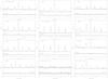 |
Fig. 1 NH3(1,1) and (2,2) spectra measured from the pre- and protostellar cores in Orion B9. The temperature scale is in TMB. NH3(2,2) spectra are offset by –1 K from zero baseline for clarity. Note that there are two velocity components towards SMM 4 and Ori B9 N, and that no lines were detected towards IRAS 05412-0105. |
3. Observational results
3.1. NH3
The NH3(1,1) and (2,2) spectra are shown in
Fig. 1. The NH3(1,1)
spectrum observed from SMM 6 with a 20 MHz bandwidth (see Sect. 2.1) is shown in
Fig. 2. In Table 2, we give the line parameters resulting from the hyperfine/Gaussian fits to the
NH3 lines. The so-called “main group optical thickness”,
τm, given in Table 2
is the sum of peak optical thicknesses of the eight hyperfine components included in the
main group. For the (1,1) transition this equals to the corresponding sum
of the ten satellite components, so the total of all peak optical thicknesses is
2 × τm. Assuming that the line profile (due to velocity
dispersion) is Gaussian, the integrated optical thickness can be obtained from
 ,
where Δv is the linewidth (FWHM) in velocity units.
The uncertainties associated with vLSR, Δv,
and τm are the 1σ fitting errors. The
uncertainty in TMB,
σ(TMB), includes the absolute calibration
uncertainty of 15%, and the 1σ rms noise in the spectrum, and was
obtained by quadratic summing of these two errors as
,
where Δv is the linewidth (FWHM) in velocity units.
The uncertainties associated with vLSR, Δv,
and τm are the 1σ fitting errors. The
uncertainty in TMB,
σ(TMB), includes the absolute calibration
uncertainty of 15%, and the 1σ rms noise in the spectrum, and was
obtained by quadratic summing of these two errors as  .
The determination of the line excitation temperature, Tex,
listed in the last column of Table 2, is described
in Sect. 4.1.1.
.
The determination of the line excitation temperature, Tex,
listed in the last column of Table 2, is described
in Sect. 4.1.1.
The NH3 spectra towards SMM 4 and Ori B9 N show evidence of a second velocity component in addition to the strong line at about 9.1 km s-1 corresponding to the systemic velocity of Orion B. In the case of IRAS 05405-0117, there is also a hint of a second velocity component, probably resulting from the fact that the 40″ beam slightly overlaps with the nearby core SMM 4. In the direction of SMM 4, the second component has a velocity of about 1.6 km s-1, whereas towards Ori B9 N the velocity is 1.9 km s-1. In both cases, the main hyperfine group of the second velocity component overlaps with the inner satellite line F1 = 1−2 of the principal velocity component. Consequently, the inner satellite line F1 = 2−1 of the second velocity component contaminates the main hyperfine group of the principal velocity component. These spectra were analysed using a two-component fit to the NH3(1,1) hyperfine structure. We note that the secondary velocity components towards SMM 4 and Ori B9 N are close to the radial velocities of IRAS 05413-0104 (1.5 km s-1) and SMM 7 (3.6 km s-1). We also note that the second velocity components influence the core parameters derived from the dust continuum emission (see Sect. 4.3). Part of the observed flux density may be due to the dust component associated with another source along the line of sight. However, because continuum observations do not provide velocity information, it is impossible to solve this “overlap” problem.
The NH3(1,1) line towards SMM 6 measured using a 20 MHz bandwidth is 30 m s-1 narrower and has a 15% larger optical thickness than that measured using a 100 MHz bandwidth. The difference in the linewidths corresponds to effect expected from instrumental broadening with the two configurations. As is expected, the product Δvτm is roughly constant at the two spectral resolutions (see Eq. (5)). As the high resolution spectrum is only available for one object, we use in the subsequent analysis the 100 MHz spectra for all of them.
3.2. N2H+
The N2H+(3−2) spectra are shown in Fig. 3. In Table 3, we show the line parameters obtained from the fits to the hyperfine structure. Here, the value of σ(TMB) includes only the 1σ rms noise in the spectrum (Col. (4) of Table 3).
The LSR velocities of the N2H+(3−2) lines are mostly similar to those determined from NH3(1,1), as can be seen in the top panel of Fig. 4. On the other hand, there is hardly any correlation between the N2H+(3−2) and NH3(1,1) linewidths (bottom panel of Fig. 4). It should be noted, however, that the hyperfine fitting to the N2H+ spectra is uncertain due to strongly overlapping components and rather a poor signal-to-noise (S/N) ratio.
The N2H+(3−2) spectra towards SMM 4 and Ori B9 N show the same lower radial velocity components (≲2 km s-1) as seen in NH3(1,1). On the other hand, the “principal component” at ~9 km s-1 is not detected towards SMM 4 and it is also very weak towards Ori B9 N. Similarly, in Paper I we found that the N2H+(1−0) spectra towards the selected position near IRAS 05405-0117/SMM 4 and Ori B9 N have second velocity components at ~1.3 and ~2.2 km s-1, respectively. The latter position also had additional N2D+(2−1) line centred at ~2.3 km s-1.
We note that Harju et al. (2006) probably detected N2H+(4−3) towards IRAS 05405-0117. They were using a double sideband system where a coincidence with DCO+(5−4) from image band could not be ruled out. Using the rest frequencies of N2H+ rotational lines from Pagani et al. (2009), the peak velocity of the suggested N2H+(4−3) line (9.25 km s-1) is very similar to that of N2H+(3−2) (9.30 km s-1). For DCO+(5−4) the peak velocity would be about 0.3 km s-1 lower (8.95 km s-1). The N2H+(4−3) linewidth (0.34 km s-1) is similar to that of NH3(1,1) (0.32 km s-1).
4. Analysis
4.1. NH3 analysis
In this subsection, we derive physical parameters from NH3 data. The obtained results are given in Col. (7) of Table 2 (Tex), and in Table 4. The analysis follows the concept first presented in 3 and further discussed in Ho et al. (1983). Here it is assumed that the same excitation temperature, Tex, characterises all the hyperfine transitions between the (1,1) and (2,2) inversion doublets.
4.1.1. Excitation, rotation, and kinetic temperatures
The Tex was calculated at the (1,1) line
peak using the optical thickness, τpeak, at that velocity,
from the equation ![\begin{equation} \label{eq:Tex} T_{\rm ex}=\frac{T_{11}}{\ln \left[1+\frac{T_{\rm MB}({v})}{T_{11}}\frac{1}{1-{\rm e}^{-\tau({v})}}+F(T_{\rm bg})\right]}, \end{equation}](/articles/aa/full_html/2010/16/aa15143-10/aa15143-10-eq75.png) (1)where
T11 = hν11/kB,
h is the Planck constant, ν11 is the
(1,1) line frequency, kB is the Boltzmann
constant, Tbg = 2.73 K is the background temperature, and
(1)where
T11 = hν11/kB,
h is the Planck constant, ν11 is the
(1,1) line frequency, kB is the Boltzmann
constant, Tbg = 2.73 K is the background temperature, and
 .
The uncertainty in Tex was calculated by propagating the
errors in the peak values of TMB(v) and
τ(v). The τ(v)
distribution was obtained using the (1,1) hyperfine fit from CLASS
which yields the LSR velocity line centroid, the width of an individual hyperfine
component, and the main group optical thickness, τm (see
Sect. 3.1).
.
The uncertainty in Tex was calculated by propagating the
errors in the peak values of TMB(v) and
τ(v). The τ(v)
distribution was obtained using the (1,1) hyperfine fit from CLASS
which yields the LSR velocity line centroid, the width of an individual hyperfine
component, and the main group optical thickness, τm (see
Sect. 3.1).
The rotational temperature, Trot, can be in principle
calculated using the formula ![\begin{equation} \label{eq:Trot2} T_{\rm rot}=\frac{-41.5}{\ln \left[\frac{3}{5}\frac{N(2,\,2)}{N(1,\,1)}\right]} , \end{equation}](/articles/aa/full_html/2010/16/aa15143-10/aa15143-10-eq85.png) (2)where
N(1,1) and N(2,2)
are the column densities of ammonia molecules at the (1,1) and
(2,2) rotational levels, respectively. The estimation of these column
densities is described in Sect. 4.1.2. The ratio 3/5 refers to the ratio of the
statistical weights of the two states
(g(1,1)/g(2,2)).
(2)where
N(1,1) and N(2,2)
are the column densities of ammonia molecules at the (1,1) and
(2,2) rotational levels, respectively. The estimation of these column
densities is described in Sect. 4.1.2. The ratio 3/5 refers to the ratio of the
statistical weights of the two states
(g(1,1)/g(2,2)).
When the optical thickness, τm, is known, Eq. (2) can be written as ![\begin{equation} \label{eq:Trot} T_{\rm rot}=\frac{-41.5}{\ln \left\{\frac{-0.283}{\tau_{\rm m}}\ln \left[1-\frac{T_{\rm MB}(2,\,2)}{T_{\rm MB}(1,\,1)}\left(1-{\rm e}^{-\tau_{\rm m}}\right)\right]\right\}} \end{equation}](/articles/aa/full_html/2010/16/aa15143-10/aa15143-10-eq89.png) (3)(Ho
et al. 1983; their Eq. (4)). Here it is assumed
that Tex and Δv are the same for both the
(1,1) and (2,2) transitions. The error associated
with Trot was propagated from the uncertainties in
TMB(1,1),
TMB(2,2), and
τm. When τm could not be
reliably determined (SMM 4, Ori B9 N, and their additional velocity components), we
estimated the NH3(1,1) and
NH3(2,2) column densities from the integrated intensities
assuming Tex = 5 K, as described below. In these cases,
Trot was also calculated using Eq. (2), and the uncertainty in
Trot was propagated from the uncertainties in the column
densities. The values of Trot calculated using Eq. (2) are mostly similar to those resulting from
Eq. (3) within the errors (see
Table 4). The subsequent analysis includes only
those Trot values which could be derived using Eq. (3).
(3)(Ho
et al. 1983; their Eq. (4)). Here it is assumed
that Tex and Δv are the same for both the
(1,1) and (2,2) transitions. The error associated
with Trot was propagated from the uncertainties in
TMB(1,1),
TMB(2,2), and
τm. When τm could not be
reliably determined (SMM 4, Ori B9 N, and their additional velocity components), we
estimated the NH3(1,1) and
NH3(2,2) column densities from the integrated intensities
assuming Tex = 5 K, as described below. In these cases,
Trot was also calculated using Eq. (2), and the uncertainty in
Trot was propagated from the uncertainties in the column
densities. The values of Trot calculated using Eq. (2) are mostly similar to those resulting from
Eq. (3) within the errors (see
Table 4). The subsequent analysis includes only
those Trot values which could be derived using Eq. (3).
NH3(1,1) and (2,2) line parameters.
The gas kinetic temperature, Tkin, was calculated from Trot using the relationship given by Tafalla et al. (2004):
 (4)This relationship is
recommended for dense cores with gas temperatures ≲20 K. Uncertainty in
Tkin was propagated from the uncertainty
in Trot.
(4)This relationship is
recommended for dense cores with gas temperatures ≲20 K. Uncertainty in
Tkin was propagated from the uncertainty
in Trot.
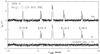 |
Fig. 2 NH3(1,1) spectrum measured from SMM 6 using the FFTS
with a 20 MHz bandwidth. Below the spectrum are shown the model fit to the
hyperfine structure and the residual spectrum. Satellite hyperfine components in
the |

4.1.2. NH3 column density calculations
The column density in the (J,K) = (1,1) state was
calculated using the formula (see Harju et al.
1993; Eqs. (3) and (5) therein)
![\begin{eqnarray} \label{eq:N11} \lefteqn {N(1,\,1)=\frac{3h\epsilon_0}{2\pi^2\mu^2}\frac{\sqrt{\pi}}{2\sqrt{\ln 2}}\frac{J(J+1)}{K^2}F(T_{\rm ex})\left({\rm e}^{T_{11}/T_{\rm ex}}+1\right)\Delta {v}\tau_{\rm tot}} \nonumber\\ &=7.83\times10^{12}F(T_{\rm ex})\left({\rm e}^{1.14/T_{\rm ex}}+1\right)\Delta {v}[{\rm km~s^{-1}}]\tau_{\rm tot}\: {\rm cm^{-2}}, \end{eqnarray}](/articles/aa/full_html/2010/16/aa15143-10/aa15143-10-eq201.png) (5)where
ϵ0 is the vacuum permittivity, μ is the
permanent electric dipole moment (1.476 D), and
τtot = 2 × τm.
(5)where
ϵ0 is the vacuum permittivity, μ is the
permanent electric dipole moment (1.476 D), and
τtot = 2 × τm.
For SMM 4 and Ori B9 N, and their second velocity components (for
which τm is uncertain in all the cases),
N(1,1) was also calculated by assuming optically
thin emission (τ ≪ 1), and using the integrated intensities of clean
satellites, i.e., those where the two velocity components do not overlap. There are
three satellite lines in the NH3(1,1) spectra of both SMM 4
and Ori B9 N that do not suffer from the contamination of the second velocity component,
i.e., F1 = 1−0, 2−1, and 0−1 (see Fig. 1). For the second velocity components, the
corresponding satellite lines are F1 = 1−0, 1−2, and
0−1. Taking into account that these lines comprise
Ri = 36.1% of the total line strength,
and assuming that the filling fraction of the emission in the beam is
ηf = 1, we can derive the formula
![\begin{eqnarray} \label{eq:N11thin} \lefteqn{N(1,\,1)=\frac{3k_{\rm B}\epsilon_0}{2\pi^2\mu^2\nu_{11}}\frac{J(J+1)}{K^2}\frac{{\rm e}^{T_{11}/T_{\rm ex}}+1}{1-\frac{F(T_{\rm bg})}{F(T_{\rm ex})}}\frac{1}{R_i}\int T_{\rm MB}(1,\,1; {\rm s}){{\rm d}v}} \nonumber\\ &=6.47\times10^{12}\frac{{\rm e}^{1.14/T_{\rm ex}}+1}{1-\frac{F(T_{\rm bg})}{F(T_{\rm ex})}}\frac{1}{R_i}\int T_{\rm MB}(1,\,1; {\rm s}){{\rm d}v} [{\rm K~km~s^{-1}}]\: {\rm cm^{-2}}, \end{eqnarray}](/articles/aa/full_html/2010/16/aa15143-10/aa15143-10-eq210.png) (6)where
TMB is integrated over the three above mentioned satellite
lines (the integrated satellite intensities are 2.53 ± 0.03 and
0.74 ± 0.03 K km s-1 for SMM 4 and Ori B9 N, respectively; for the
corresponding second velocity components, the values are 2.18 ± 0.02 and
1.18 ± 0.03 K km s-1, respectively). For this calculation, the excitation
temperature was assumed to be 5 K for both SMM 4 and Ori B9 N (and their second velocity
components). This assumption is similar to the values calculated from Eq. (1) in all the other cases except the
principal velocity component towards SMM 4, where Tex might
be >5 K (see Col. (7) of Table 2). Similarly, N(2,2) (needed in the
calculation of Trot using Eq. (2)) was calculated by assuming that τ ≪ 1, and using
the integrated intensity of the main (2,2) hyperfine complex, which
accounts for Ri = 79.63% of the total line
strength. In this case, we can write
(6)where
TMB is integrated over the three above mentioned satellite
lines (the integrated satellite intensities are 2.53 ± 0.03 and
0.74 ± 0.03 K km s-1 for SMM 4 and Ori B9 N, respectively; for the
corresponding second velocity components, the values are 2.18 ± 0.02 and
1.18 ± 0.03 K km s-1, respectively). For this calculation, the excitation
temperature was assumed to be 5 K for both SMM 4 and Ori B9 N (and their second velocity
components). This assumption is similar to the values calculated from Eq. (1) in all the other cases except the
principal velocity component towards SMM 4, where Tex might
be >5 K (see Col. (7) of Table 2). Similarly, N(2,2) (needed in the
calculation of Trot using Eq. (2)) was calculated by assuming that τ ≪ 1, and using
the integrated intensity of the main (2,2) hyperfine complex, which
accounts for Ri = 79.63% of the total line
strength. In this case, we can write
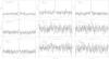 |
Fig. 3 N2H+(3−2) spectra measured from the pre- and protostellar cores in Orion B9. Spectra are overlaid with the 38 component hyperfine structure fits. Hyperfine fits to the second velocity components are indicated by red lines. Note that only the second velocity component is detected towards SMM 4. The relative velocity of each individual hyperfine component is labelled with a short bar on the spectrum towards IRAS 05399-0121 (top left panel). The temperature scale is in TMB. |
![\begin{eqnarray} \label{eq:N22thin} \lefteqn{N(2,\,2)=\frac{3k_{\rm B}\epsilon_0}{2\pi^2\mu^2\nu_{22}}\frac{J(J+1)}{K^2}\frac{{\rm e}^{T_{22}/T_{\rm ex}}+1}{1-\frac{F(T_{\rm bg})}{F(T_{\rm ex})}}\frac{1}{R_i}\int T_{\rm MB}(2,\,2; {\rm m}){{\rm d}v}} \nonumber\\ &=4.85\times10^{12}\frac{{\rm e}^{1.14/T_{\rm ex}}+1}{1-\frac{F(T_{\rm bg})}{F(T_{\rm ex})}}\frac{1}{R_i}\int T_{\rm MB}(2,\,2; {\rm m}){{\rm d}v}[{\rm K~km~s^{-1}}]\: {\rm cm^{-2}}, \end{eqnarray}](/articles/aa/full_html/2010/16/aa15143-10/aa15143-10-eq217.png) (7)where
ν22 is the (2,2) line frequency, and
T22 = hν22/kB.
The integrated intensities of the (2,2) main line for SMM 4 and Ori
B 9 N are 0.21 ± 0.01 and 0.05 ± 0.01 K km s-1, respectively (0.15 ± 0.01 and
0.21 ± 0.03 K km s-1 for the corresponding second velocity components). The
uncertainties associated with N(1,1) and
N(2,2) were propagated from the formal errors in the
integrated intensities.
(7)where
ν22 is the (2,2) line frequency, and
T22 = hν22/kB.
The integrated intensities of the (2,2) main line for SMM 4 and Ori
B 9 N are 0.21 ± 0.01 and 0.05 ± 0.01 K km s-1, respectively (0.15 ± 0.01 and
0.21 ± 0.03 K km s-1 for the corresponding second velocity components). The
uncertainties associated with N(1,1) and
N(2,2) were propagated from the formal errors in the
integrated intensities.
The total NH3 column density, N(NH3), was
calculated by scaling the column density in the (1,1) state by the
ratio
N(NH3)/N(1,1)
obtained from the partition function Z. This yields approximately
(e.g., Rosolowsky et al. 2008; Busquet et al. 2009) 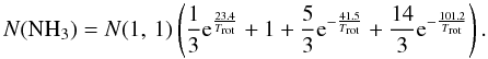 (8)The uncertainty in
N(NH3) was calculated by propagating the errors associated
with Tex, Δv,
τm, and Trot. The values of
N(NH3) calculated by substituting
N(1,1) from Eq. (6) into Eq. (8) are
mostly in good agreement, within the errors, with those resulting from Eqs. (5) and (8). In the subsequent analysis, we only use NH3 column
densities derived for each source from Eqs. (5) and (8) to keep the data set
homogeneous (see Col. (4) of Table 4).
(8)The uncertainty in
N(NH3) was calculated by propagating the errors associated
with Tex, Δv,
τm, and Trot. The values of
N(NH3) calculated by substituting
N(1,1) from Eq. (6) into Eq. (8) are
mostly in good agreement, within the errors, with those resulting from Eqs. (5) and (8). In the subsequent analysis, we only use NH3 column
densities derived for each source from Eqs. (5) and (8) to keep the data set
homogeneous (see Col. (4) of Table 4).
4.1.3. Fractional NH3 abundance
The fractional NH3 abundance was calculated by dividing the total NH3 column density by the H2 column density, i.e., x(NH3) = N(NH3)/N(H2). The H2 column densities were determined from the submm dust continuum emission (Paper I; Eq. (3) therein), using the kinetic temperatures derived in the present paper and assuming that Tkin = Tdust (see also Sect. 4.3). We smoothed the LABOCA 870 μm map to correspond the 40″ resolution of the Effelsberg NH3 observations.
N2H+(3−2) line parameters.
4.1.4. Non-thermal velocity dispersion and the level of internal turbulence
The measured NH3(1,1) linewidths were used to calculate the
non-thermal portion of the line-of-sight velocity dispersion (averaged over a ~40″
beam), and the level of internal turbulence. The observed velocity dispersion is related
to the FWHM linewidth as  .
The non-thermal velocity dispersion can then be calculated as follows:
.
The non-thermal velocity dispersion can then be calculated as follows: 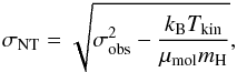 (9)where
μmol is the mass of the emitting molecule in units of
atomic mass number (17 for NH3), and mH is the
mass of the hydrogen atom. Furthermore, the level of internal turbulence is given by
fturb = σNT/cs,
where cs is the one-dimensional isothermal sound speed
(0.19 km s-1 in a 10 K H2 gas with 10% He). The errors in
σNT and fturb were derived by
propagating the errors in Δv and Tkin.
(9)where
μmol is the mass of the emitting molecule in units of
atomic mass number (17 for NH3), and mH is the
mass of the hydrogen atom. Furthermore, the level of internal turbulence is given by
fturb = σNT/cs,
where cs is the one-dimensional isothermal sound speed
(0.19 km s-1 in a 10 K H2 gas with 10% He). The errors in
σNT and fturb were derived by
propagating the errors in Δv and Tkin.
Parameters derived from NH3 data.
4.2. N2H+ analysis
In this subsection, we derive physical parameters from N2H+ data. The obtained results are given in Col. (6) of Table 3 (Tex), and in Table 5.
4.2.1. Tex, σNT, and fturb
The excitation temperature of the N2H+(3−2) transition was calculated as in the case of NH3(1,1) (see Eq. (1)). The optical thickness, and thus Tex, could be determined only for three sources: IRAS 05399-0121, and SMM 1 and 3. For the rest of the sources, it was assumed that Tex = 5 K, and τtot was then estimated using this value. The value Tex = 5 K is expected to be a reasonable choice because for the above three sources Tex is around 5 kelvins.
The values of σNT and fturb were calculated as in the case of NH3(1,1) (see Eq. (9)), by using the values of Tkin from NH3 measurements. For N2H+, μmol is 29.
4.2.2. N2H+ column density and fractional abundance
The N2H+ column density was calculated using the formula (see,
e.g., Paper I)
![\begin{eqnarray} \label{eq:Ntot2} \lefteqn {N({\rm N_2H^+})=\frac{3h\epsilon_0}{2\pi^2\mu^2}\frac{\sqrt{\pi}}{2\sqrt{\ln 2}}\frac{1}{J_{\rm u}}{\rm e}^{E_{\rm u}/k_{\rm B}T_{\rm ex}}F(T_{\rm ex})Z(T_{\rm ex})\Delta {v}\tau_{\rm tot}} \nonumber\\ &=2.46\times10^{11}{\rm e}^{26.83/T_{\rm ex}}F(T_{\rm ex})Z(T_{\rm ex})\Delta {v}[{\rm km~s^{-1}}]\tau_{\rm tot}\: {\rm cm^{-2}}, \end{eqnarray}](/articles/aa/full_html/2010/16/aa15143-10/aa15143-10-eq374.png) (10)where
μ is 3.4 D, the upper rotational level number
Ju = 3,
Eu = hBJu(Ju + 1)
is the energy of the upper transition state, and B = 46586.8713 MHz is
the rotational constant (Pagani et al. 2009). The
rotational partition function was approximated by
(10)where
μ is 3.4 D, the upper rotational level number
Ju = 3,
Eu = hBJu(Ju + 1)
is the energy of the upper transition state, and B = 46586.8713 MHz is
the rotational constant (Pagani et al. 2009). The
rotational partition function was approximated by  .
.
In those cases where the line was optically thin (i.e., SMM 5, Ori B9 N and its second
velocity component, and SMM 7), the N2H+ column density was also
calculated from the integrated intensity. The integrated intensities obtained from
Gaussian fits are 0.15 ± 0.03, 0.07 ± 0.16 (0.12 ± 0.04), and
0.22 ± 0.07 K km s-1 for SMM 5, Ori B9 N (and its second velocity
component), and SMM 7, respectively. Note that the error is larger than the value for
Ori B9 N. By combining Eqs. (4) and (6) of Paper I, we get the following formula for the
N(N2H+) as a function of integrated
intensity:
![\begin{eqnarray} \label{eq:Ntot3} \lefteqn {N({\rm N_2H^+})=\frac{3\epsilon_0 k_{\rm B}}{2\pi^2\mu^2\nu}\frac{1}{J_{\rm u}}{\rm e}^{E_{\rm u}/k_{\rm B}T_{\rm ex}}Z(T_{\rm ex})\frac{1}{1-\frac{F(T_{\rm bg})}{F(T_{\rm ex})}}\int T_{\rm MB}{{\rm d}v}} \nonumber\\ &=1.72\times10^{10}Z(T_{\rm ex})\frac{{\rm e}^{26.83/T_{\rm ex}}}{1-\frac{F(T_{\rm bg})}{F(T_{\rm ex})}}\int T_{\rm MB}{{\rm d}v}[{\rm K~km~s^{-1}}]\: {\rm cm^{-2}} . \end{eqnarray}](/articles/aa/full_html/2010/16/aa15143-10/aa15143-10-eq384.png) (11)When
applying Eq. (11), it was taken into
account that the detectable emission feature with 24 hyperfine components contains 92.6%
of the total line strength. The values of
N(N2H+) calculated from Eqs. (10) and (11) are similar to each other within the errors (see Table 5).
(11)When
applying Eq. (11), it was taken into
account that the detectable emission feature with 24 hyperfine components contains 92.6%
of the total line strength. The values of
N(N2H+) calculated from Eqs. (10) and (11) are similar to each other within the errors (see Table 5).
The fractional N2H+ abundance was calculated in a similar manner as for NH3. In this case, the LABOCA map was smoothed to the resolution of the N2H+ observations (22″̣3).
Parameters derived from N2H+(3−2) data.
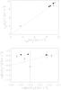 |
Fig. 4 Top: the centroid velocity of the N2H+(3−2) emission versus the velocity of the NH3(1,1) emission. Bottom: Log-log plot of the N2H+(3−2) linewidth versus the NH3(1,1) linewidth. Prestellar cores are indicated by open diamonds and protostellar cores are marked by filled diamonds. In both plots, the dashed line shows the equality. |
4.3. Revision of core properties presented in Paper I
In Paper I, we assumed that the dust temperature is
Tdust = 10 K for the starless cores, whereas for protostellar
cores we used the temperatures derived from the spectral energy distribution (SED) fits
(Table 6 in Paper I). By using the gas kinetic temperatures determined in the present
paper, we recalculated several parameters presented in Paper I, by assuming that
Tkin = Tdust. These include the
core mass, M, H2 column density,
N(H2), and the average H2 number density,
⟨ n(H2) ⟩ . In the present paper, we have also amended some
formula used in the derivation of the physical parameters: in the calculation of
⟨ n(H2) ⟩ , we have used the effective radius
 (instead of the FWHM radius used in Paper I), and the value
2.8mH for the mean molecular weight per
H2 molecule (instead of 2.33mH which is the mean
particle weight in an H2 + 10% He mixture). The former change is motivated by
the fact that the flux densities used to calculate the core masses refer to their
projected areas, A. The results of these calculations are presented in
Table 6. The revised values of M
and N(H2), are, on average, about 11% and 9% higher than those
reported in Paper I. On the other hand, the new average densities,
⟨ n(H2) ⟩ , are only about 1/5 of those calculated in
Paper I. Note that the total mass of the cores is still
~50 M⊙, i.e., about 4% of the total mass in the region
(Paper I).
(instead of the FWHM radius used in Paper I), and the value
2.8mH for the mean molecular weight per
H2 molecule (instead of 2.33mH which is the mean
particle weight in an H2 + 10% He mixture). The former change is motivated by
the fact that the flux densities used to calculate the core masses refer to their
projected areas, A. The results of these calculations are presented in
Table 6. The revised values of M
and N(H2), are, on average, about 11% and 9% higher than those
reported in Paper I. On the other hand, the new average densities,
⟨ n(H2) ⟩ , are only about 1/5 of those calculated in
Paper I. Note that the total mass of the cores is still
~50 M⊙, i.e., about 4% of the total mass in the region
(Paper I).
In Paper I, we compared the core mass distributions in Orion B9 and Orion B North studied by Nutter & Ward-Thompson (2007) (Sect. 5.2 and Fig. 7 in Paper I). The core mass functions (CMFs) were constructed by removing the Class I protostellar cores from the samples (i.e., IRAS 05399-0121 was removed from the Orion B9 core sample). We performed a two-sample Kolmogorov-Smirnov (K-S) test between the two CMFs to examine if they represent the subsamples of the same underlying parent distribution. For this purpose, the masses were scaled to compensate for the different assumptions about the distance, dust temperature, and opacity. We found a very high likelihood of ~95% for the null hypothesis that the two CMFs are drawn from the same parent distribution (i.e., the probability that the two samples do not have the same parent distribution is 1−0.95 = 0.05). We repeated this analysis by using the updated masses listed in Col. (3) of Table 6. In this case, a K-S test yielded a probability of ~100%, strengthening the possibility that the core masses in these two different parts of Orion B are drawn from the same distribution.
4.4. Virial masses
In order to study the stability of the cores, we calculated their virial masses using the
following formula where the effects of external pressure and magnetic field are ignored:
 (12)where
G is the gravitational constant, and Δvave
is the width of the spectral line emitted by the molecule of mean mass
μ = 2.33. The parameter
a = (1 − p/3)/(1 − 2p/5),
wherep is the power-law index of the density profile
(n(r) ∝ r − p),
is a correction for deviations from constant density. For starless cores we used the value
p = 1.0, whereas for protostellar cores we set p = 1.5
(see Paper I). The value of Mvir calculated with
p = 1.0 is about 13% higher compared to that calculated with the value
p = 1.5. As a function of the observed linewidth,
Δvobs (Table 2,
Col. (4)), Δvave is given by
(12)where
G is the gravitational constant, and Δvave
is the width of the spectral line emitted by the molecule of mean mass
μ = 2.33. The parameter
a = (1 − p/3)/(1 − 2p/5),
wherep is the power-law index of the density profile
(n(r) ∝ r − p),
is a correction for deviations from constant density. For starless cores we used the value
p = 1.0, whereas for protostellar cores we set p = 1.5
(see Paper I). The value of Mvir calculated with
p = 1.0 is about 13% higher compared to that calculated with the value
p = 1.5. As a function of the observed linewidth,
Δvobs (Table 2,
Col. (4)), Δvave is given by  (13)The virial masses are
listed in Col. (4) of Table 6. The associated error
was propagated from those of Δvobs and
Tkin.
(13)The virial masses are
listed in Col. (4) of Table 6. The associated error
was propagated from those of Δvobs and
Tkin.
The virial parameters of the cores were calculated following 1, i.e., αvir = Mvir/M. The uncertainty was derived by propagating the errors in both mass estimates. The values are given in Col. (5) of Table 6. Note that αvir = 1 corresponds to the virial equilibrium, 2 ⟨ T ⟩ = −⟨ U ⟩ , where T and U are the internal kinetic and gravitational energies, respectively. The value αvir = 2 corresponds to the self-gravitating limit defined by ⟨ T ⟩ = −⟨ U ⟩ .
Revised core parameters presented in Paper I.
5. Discussion
5.1. The gas kinetic temperature in dense cores in Orion B
The gas kinetic temperatures within the cores in Orion B9 are in the range ~9.4−13.9 K, with a mean value of 12.0 ± 0.4 K (the quoted error is the standard deviation of the mean). The highest temperatures (13.4–13.9 K) are found towards IRAS 05399-0121, SMM 4, Ori B9 N, and IRAS 05413-0104. There is, however, no such tendency that the warmest cores should be protostellar. For example, the Class 0 sources SMM 3 and IRAS 05405-0117 have Tkin values at the low end in the sample (11.3 K for both sources). This is consistent with the notion that embedded low-mass protostars do not heat significantly the parent cores, but the heating is localised in their immediate vicinity (≲100 AU; Friesen et al. 2010 and references therein).
Recently, based on the Nobeyama 45-m observations, Ikeda et al. (2009) derived the
NH3 rotational temperatures towards 144 positions in Orion B. The cores
No. 55-66 in the Ikeda et al. (2009) sample lie in the Orion B9 region. For these latter
cores, they found the values in the range
Trot = 10.1−16.1 K. By using the relationship (4), this corresponds to the
Tkin values 10.6−18.5 K, with the mean value 16.4 K. This
is clearly higher than the mean Tkin of the present study. The
difference is likely to be caused by the larger beamsize used by Ikeda et al.
( ). We note that the highest value of
Tkin = 43.9 K in the Ikeda et al. (2009) sample was found in
the NGC 2024 H ii region, and the lowest values (≲ 11 K) were found in Orion B9
and other regions of relatively low star formation activity, i.e., outside the NGC 2023,
2024, 2068, and 2071 regions.
). We note that the highest value of
Tkin = 43.9 K in the Ikeda et al. (2009) sample was found in
the NGC 2024 H ii region, and the lowest values (≲ 11 K) were found in Orion B9
and other regions of relatively low star formation activity, i.e., outside the NGC 2023,
2024, 2068, and 2071 regions.
We note that in several previous submm surveys of Orion B dust temperatures around 20 K have been derived or assumed for dense cores (Johnstone et al. 2001, 2006; Nutter & Ward-Thompson 2007). Together with the results of Ikeda et al. (2009) the present temperature determinations demonstrate that Orion B contains also several very cold cores resembling cores in nearby low-mass star forming regions (see, e.g., Rosolowsky et al. 2008; Schnee et al. 2009; Friesen et al. 2009 and references therein).
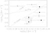 |
Fig. 5 Non-thermal versus thermal (for H2, i.e., the isothermal sound speed) linewidths in log-log scales. The dashed line indicates ΔvNT = ΔvT. The dotted and dash-dotted lines show relationships found by 4 for NH3 cores with and without cluster association, respectively. Symbols have the same meaning as in Fig. 4. |
5.2. Kinematics of the core gas
The NH3 line profiles show that most cores have subsonic non-thermal motions (fturb < 1). In two cores (SMM 1 and 7), fturb is higher than in the rest of the cores, and non-thermal motions appear to be slightly transonic (fturb = 1.3 < 2). Recently, Friesen et al. (2009) found that the mean fturb value for dense cores in Oph B is 1.5, clearly larger than the corresponding value for our cores (a mean fturb and its standard deviation is 0.8 ± 0.1).
In Fig. 5, we plot the non-thermal linewidth against the thermal linewidth for the cores. Figure 5 shows that most of the cores in Orion B9 are quiescent, i.e., ΔvNT < ΔvT. Also shown in this figure are the ΔvNT−ΔvT relationships found by 4 for NH3 cores in clusters and isolated regions. The two relationships suggest that non-thermal NH3 linewidths are larger for cores in clustered environments than in isolated cores. A majority of Orion B9 cores lie on the Jijina plot in the region characteristic of isolated cores.
Like in the case of the kinetic temperature, there is no clear difference in linewidths between starless and protostellar cores. Protostars are likely to be associated with outflows which could cause the linewidths to be larger, but evidence for outflows can only be found in IRAS 05399-0121 (HH 92; Bally et al. 2002) and IRAS 05413-0104 (HH 212; e.g., Lee et al. 2008). It is possible that the HH 92 outflow from IRAS 05399-0121 contribute to the relatively broad NH3 lines seen in the adjacent SMM 1 core which is oriented along the direction of the outflow.
In Fig. 6, we plot the NH3(1,1) linewidth as a function of core effective radius. Also shown are the linewidth-size relation derived by 5, and the relationship recently found by Ikeda et al. (2009) for the H13CO+ cores in Orion B. The Larson relation, thought to arise from the interstellar turbulence, was originally presented for the 3D velocity dispersion, σ3D, and the maximum linear size of the source, L. In terms of our definitions, it can be written as Δv [km s-1] = 1.9(Reff [pc] )0.38, where we have assumed that L = 2Reff. The linewidths of Orion B9 cores mostly deviate downward from the Larson relation, and the cores lie around the Ikeda et al. (2009) relationship, namely Δv [km s-1] = 1.28(Rcore [pc] )0.38 (we remind the reader that the Ikeda et al. sample contains Orion B9 members). On the other hand, it is possible that the more tenuous gas in Orion B9 follows the Larson relation: the mean linewidth (~1.3 km s-1) and half-maximum radius (~0.6 pc) measured from the 13CO(1−0) emission towards the Orion B9 region by 2 are quite similar to those expected from the Larson relation. As pointed out by Maruta et al. (2010), this could be explained if the cores were formed in regions where supersonic turbulence was dissipated. Dissipation of turbulence could be due to shocks in the converging turbulent flows, where the formation of density enhancements is expected to take place (see Sect. 5.9). The timescale for the dissipation of turbulence in dense cores is comparable to the free-fall timescale (e.g., Mac Low & Klessen 2004). Thus, because the observed linewidth-size relation appears to be quite flat, it is possible that the turbulent gas motions at small scales (≲0.1 pc) are not yet settled into equilibrium state (i.e., relaxed). In this case, the core formation should be a rapid process with the corresponding timescale being comparable to the free-fall time.
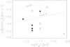 |
Fig. 6 Linewidth versus radius for the cores in Orion B9 in log-log scales. The 5 relation is shown by the dotted line. The dashed line indicates the relation derived by Ikeda et al. (2009) for the H13CO+ cores in Orion B. Symbols have the same meaning as in Fig. 4. |
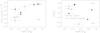 |
Fig. 7 Left: total internal kinetic gas pressure versus core mass. Right: the ratio of thermal to non-thermal pressure as a function of mass. The dashed horizontal line marks the point at which thermal and non-thermal pressure support are equal. Both plots are in log-log scales, and the symbols have the same meaning as in Fig. 4. |
5.3. Internal pressure support
The internal kinetic gas pressure, Pint, within the core
consists of a thermal pressure,
pT = nkBTkin,
and a non-thermal pressure,  , where
n is the number density, and μ = 2.33
(Pint = pT + pNT).
In the left panel of Fig. 7, we plot
Pint/kB
versus core mass. Excluding the one outlier in the plot (SMM 6), there is a trend of
increasing internal pressure with increasing core mass. This indicates that the cores are
not in pressure equilibrium with an external pressure due to, e.g., the weight of the
cloud in which the cores are embedded (Lada et al.
2008). The mean internal pressure of the Orion B9 core population is
~1.1 × 10⁶ K cm-3. This is in excellent agreement with the value
~106 K cm-3 estimated by Johnstone et al. (2001) for the cores
in the northern part of Orion B. For comparison, the overall pressure of the ISM in the
Galactic midplane, which consists of thermal and turbulent kinetic pressures, and the
pressures of magnetic fields and cosmic rays, has been estimated to be
PISM/kB ≈ 2.8 × 10⁴ K cm-3
(Boulares & Cox 1990). The high pressures
inside cores are likely to result from compression by gravity (see Sect. 5.4).
, where
n is the number density, and μ = 2.33
(Pint = pT + pNT).
In the left panel of Fig. 7, we plot
Pint/kB
versus core mass. Excluding the one outlier in the plot (SMM 6), there is a trend of
increasing internal pressure with increasing core mass. This indicates that the cores are
not in pressure equilibrium with an external pressure due to, e.g., the weight of the
cloud in which the cores are embedded (Lada et al.
2008). The mean internal pressure of the Orion B9 core population is
~1.1 × 10⁶ K cm-3. This is in excellent agreement with the value
~106 K cm-3 estimated by Johnstone et al. (2001) for the cores
in the northern part of Orion B. For comparison, the overall pressure of the ISM in the
Galactic midplane, which consists of thermal and turbulent kinetic pressures, and the
pressures of magnetic fields and cosmic rays, has been estimated to be
PISM/kB ≈ 2.8 × 10⁴ K cm-3
(Boulares & Cox 1990). The high pressures
inside cores are likely to result from compression by gravity (see Sect. 5.4).
To examine the relative role of turbulence in the core internal pressure, we calculated
the ratio of thermal to non-thermal pressure, which is given by  (see Sect. 4.1.4). The values
of Rp are plotted as a function of mass in the right panel
of Fig. 7. As can be seen in this figure, thermal
pressure is clearly the dominant source of internal gas pressure for 8 of 11 cores. For
the rest of the cores, thermal pressure support is still significant as they have
Rp > 0.5. Also in this regard, the
Orion B9 cores appear to be similar to low-mass dense cores in nearby molecular clouds,
which are commonly found to be thermally dominated (e.g., Myers & Benson 1983; Kirk et al.
2007; Lada et al. 2008).
(see Sect. 4.1.4). The values
of Rp are plotted as a function of mass in the right panel
of Fig. 7. As can be seen in this figure, thermal
pressure is clearly the dominant source of internal gas pressure for 8 of 11 cores. For
the rest of the cores, thermal pressure support is still significant as they have
Rp > 0.5. Also in this regard, the
Orion B9 cores appear to be similar to low-mass dense cores in nearby molecular clouds,
which are commonly found to be thermally dominated (e.g., Myers & Benson 1983; Kirk et al.
2007; Lada et al. 2008).
5.4. Dynamical state and gravitational boundedness of the cores
To further examine the dynamical state of the cores, we inspect the virial parameters derived in Sect. 4.4. Figure 8 (left panel) shows the distribution of the virial parameter for the Orion B9 cores as a function of mass. Within the errors, all eleven cores are self-gravitating (αvir < 2), and five of them seem to be close to the virial equilibrium or collapsing (αvir ≤ 1). One should note that the virial calculation presented above did not include any external pressure or magnetic fields. An external presssure of Pext/kB ~ 2−3 × 10⁵ K cm-3 would bring all starless cores except SMM 7 to virial equilibrium or make them collapse (neglecting the possible magnetic support). Assuming that the gas surrounding the cores is characterised by σNT ~ 0.6 km s-1 and n(H2) = 2 × 103 cm-3, corresponding to the typical width of 13CO(1−0) lines observed by 2 in this region and the critical density of the transition in question (which is lower than the critical density of the NH3 inversion lines), its turbulent ram pressure would roughly equal to the required confining pressure quoted above. As discussed by Lada et al. (2008) in the case of Pipe Nebula, the supersonic intercore turbulence can be a manifestation of the self-gravity of the surrounding massive cloud.
It seems likely that most if not all starless cores in Orion B9 detected in this survey are prestellar, i.e. they will eventually collapse to stars. The situation resembles that observed in Perseus by Foster et al. (2009): most cores are gravitationally bound, and ~1/3 are in virial equilibrium.
The virial parameter, αvir seems to decrease as a function of core mass (see Fig. 8, left). The slope of a least-squares fit, log (αvir) = (0.54 ± 0.10) − (0.67 ± 0.16)log (M), with the linear correlation coefficient r = −0.81, is very close to that found by Lada et al. (2008) for cores in the Pipe Nebula which are believed to be predominantly confined by external pressure. Our cores with masses in the range 2−8 M⊙ correspond to the most massive Pipe cores. The slope (~−2/3) is consistent with the theoretical prediction of 1 for pressure confined cores, and basically results from the fact that there is not much core-to-core variation in the average densities and velocity dispersions. It should be noted, however, that the overall level of αvir, characterised by the constant of the fit, is lower than derived in the Pipe, probably reflecting the different environments and evolutionary stages of the two regions.
Like Lada et al. (2008) we have also plotted in the right panel of Fig. 8 the correlation diagram between the ratio
σ3D/vesc and
the core mass, where the three-dimensional velocity dispersion,
σ3D, is calculated from  ,
and the escape velocity, vesc is given by
,
and the escape velocity, vesc is given by
 .
For all cores, σ3D is smaller than
vesc, supporting the above conclusion that the cores are
gravitationally bound. Morever, the
σ3D/vesc
ratio appears to decrease as a function of core mass. A least-squares fit to the whole
sample gives
.
For all cores, σ3D is smaller than
vesc, supporting the above conclusion that the cores are
gravitationally bound. Morever, the
σ3D/vesc
ratio appears to decrease as a function of core mass. A least-squares fit to the whole
sample gives  , with r = −0.94. This
relationship implies that the transition from unbound to bound core occurs at about
0.8–0.9 M⊙. This is very close to the peak of the CMF for
Orion B North, i.e., ~1 M⊙ (Nutter & Ward-Thompson 2007). This is expected because the CMFs
for Orion B9 and Orion B North seem to represent the subsamples of the same parent
distribution (Sect. 4.3). A similar correspondence was found by Lada et al. (2008) for the
dense cores in the Pipe Nebula.
, with r = −0.94. This
relationship implies that the transition from unbound to bound core occurs at about
0.8–0.9 M⊙. This is very close to the peak of the CMF for
Orion B North, i.e., ~1 M⊙ (Nutter & Ward-Thompson 2007). This is expected because the CMFs
for Orion B9 and Orion B North seem to represent the subsamples of the same parent
distribution (Sect. 4.3). A similar correspondence was found by Lada et al. (2008) for the
dense cores in the Pipe Nebula.
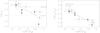 |
Fig. 8 Left: virial parameter versus core mass. The dashed line indicates the virial equilibrium limit (αvir = 1), and the dash-dotted line shows the limit of gravitational boundedness (αvir = 2). Right: ratio of 3D velocity dispersion to escape velocity against core mass. The dashed line indicates σ3D/vesc = 1. All cores are likely to be gravitationally bound. The solid line in both plots indicates the least-squares fit to the data. Both plots are in log-log scales, and the symbol key is identical to that of Fig. 4. |
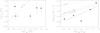 |
Fig. 9 Left: Tkin versus Tbol. The dashed line indicates Tkin = Tbol. Right: ΔvNT versus Lbol. The solid line indicates the least-squares fit to the data. The upper and lower dashed lines represent relationships found by 4 for NH3 cores with and without cluster association, respectively. The dash-dotted line shows the relationships found by Myers et al. (1991) for IRAS point sources. Both plots are in log-log scales. |
5.5. Correlating the properties of protostellar cores
In Paper I, we derived the SEDs for the protostellar cores in Orion B9. For all sources, the observed flux densities were fitted by a two-temperature (warm + cold) composite model. The bolometric dust temperatures and bolometric luminosities of the sources derived from the SEDs are given in Table 6 of Paper I.
In the left panel of Fig. 9, we show the correlation plot between Tkin and the bolometric temperature, Tbol. Only for SMM 3, the two values are similar within the errors, and in the case of SMM 4, Tkin and Tbol agree within a few kelvins. For the other sources (i.e., the three IRAS sources), however, the temperatures estimated from the SEDs are clearly higher than those obtained from NH3 measurements. The SEDs of SMM 3 and 4 were constructed by using only three flux density values at 24, 70, and 870 μm (see Paper I; Fig. 6 therein). In the case of other sources, also the flux densities at all four IRAS bands (12, 25, 60, and 100 μm) were included in the SED fits. This may have caused the temperature of the cold part of the spectrum to be overestimated. Shetty et al. (2009) recently concluded that if using flux density values at widely separated wavelengths, and including short-wavelength flux densities in the SED fit, the obtained temperatures may be too high.
The right panel of Fig. 9 shows a plot of
ΔvNT as a function of Lbol.
There appears to be a positive correlation between the two quantities, and the
least-squares linear fit to the data gives
log (ΔvNT) = (−0.65 ± 0.10) + (0.25 ± 0.11)log (Lbol),
with r = 0.80. We also show the relationships found by 4 for NH3 cores in clusters and cores
without cluster association (see their Table B7), and the Myers et al. (1991) relation for a sample of 61 IRAS point sources
(their Eq. (3)). Our result is similar to the relationship found in the latter two
studies,  . The
fact that ΔvNT increases as a function of
Lbol can be explained by the effects of winds driven by the
embedded protostar + disk system, and by the fact that more turbulent initial conditions
give rise to more massive, i.e., more luminous stars (Myers et al. 1991). As in the case of
ΔvNT − ΔvT relation (see
Fig. 5), the Orion B9 cores more closely follow the
relationship for isolated cores.
. The
fact that ΔvNT increases as a function of
Lbol can be explained by the effects of winds driven by the
embedded protostar + disk system, and by the fact that more turbulent initial conditions
give rise to more massive, i.e., more luminous stars (Myers et al. 1991). As in the case of
ΔvNT − ΔvT relation (see
Fig. 5), the Orion B9 cores more closely follow the
relationship for isolated cores.
5.6. Column densities and fractional abundances of NH3 and N2H+
The mean NH3 fractional abundance in our sample is 4.8 ± 0.7 × 10⁻⁸, where the ±-error represents the standard deviation of the mean. The value of ⟨x(NH3)⟩ in Orion B9 is similar to those recently found by Foster et al. (2009) and Friesen et al. (2009) for the dense cores in Perseus and Ophiuchus, respectively (i.e., a few to several × 10-8). For comparison, the NH3 abundances in dense cores in nearby regions of isolated star formation, such as Taurus, are commonly found to be ~0.4−5 × 10⁻⁸ (e.g., Hotzel et al. 2001; Tafalla et al. 2002, 2006). The average N2H+ abundance in Orion B9, ⟨x(N2H+)⟩ = 2.5 ± 0.8 × 10⁻¹⁰, is very similar to those in isolated low-mass cores (e.g., ⟨x(N2H+)⟩ = 2 ± 1 × 10⁻¹⁰ and 3 ± 2 × 10⁻¹⁰ for the starless and protostellar core samples of Caselli et al. (2002)). On the other hand, the value of ⟨x(N2H+)⟩ is about 2–6 times lower than those determined by Friesen et al. (2010) in the Oph B1 and B2 cores which lie in the region of clustered star formation.
As shown in the left panel of Fig. 10, the
fractional NH3 abundance appears to decrease with increasing H2
column density (as traced by 870 μm continuum emission smoothed to 40″
resolution). A linear-least-squares fit to the data gives
log x(NH3) = (4.2 ± 6.6)−(0.5 ± 0.3)log N(H2),
with r = −0.51. The slope of this relationship,
 ,
is very similar to that found by Friesen et al. (2009, 2010) in the Oph B2 core. In the
middle panel of Fig. 10, we plot
x(NH3) as a function of n(H2).
The trend is similar as above, and the least-squares linear fit to the data indicates
log x(NH3) = (−4.5 ± 1.4)−(0.6 ± 0.3)log n(H2),
with r = −0.57. The tendencies described above are likely to manifest
the fact that NH3, like species containing carbon or oxygen, accrete onto grain
surfaces at high densities. According to chemistry models of Aikawa et al. (2005) and
Flower et al. (2006), the NH3 abundance becomes heavily depleted at densities
nH ≳ a few × 106 cm-3 (due to
freeze-out of the parent species N2). The
x(NH3) − n(H2) relationship
shown in Fig. 10 agrees reasonably well with the
predictions for the early stages of collapse presented in Flower et al. (2006; see, e.g.,
their Fig. 4). In the Flower et al. model, the protostellar collapse occurs on the
free-fall timescale which is about 4 × 10⁵ yr at
nH = 104 cm-3. This is in agreement
with statistical estimates of the prestellar core lifetime (see Sect. 5.9).
,
is very similar to that found by Friesen et al. (2009, 2010) in the Oph B2 core. In the
middle panel of Fig. 10, we plot
x(NH3) as a function of n(H2).
The trend is similar as above, and the least-squares linear fit to the data indicates
log x(NH3) = (−4.5 ± 1.4)−(0.6 ± 0.3)log n(H2),
with r = −0.57. The tendencies described above are likely to manifest
the fact that NH3, like species containing carbon or oxygen, accrete onto grain
surfaces at high densities. According to chemistry models of Aikawa et al. (2005) and
Flower et al. (2006), the NH3 abundance becomes heavily depleted at densities
nH ≳ a few × 106 cm-3 (due to
freeze-out of the parent species N2). The
x(NH3) − n(H2) relationship
shown in Fig. 10 agrees reasonably well with the
predictions for the early stages of collapse presented in Flower et al. (2006; see, e.g.,
their Fig. 4). In the Flower et al. model, the protostellar collapse occurs on the
free-fall timescale which is about 4 × 10⁵ yr at
nH = 104 cm-3. This is in agreement
with statistical estimates of the prestellar core lifetime (see Sect. 5.9).
 |
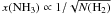
Fig. 10 Comparison of chemical abundances as a function of H2 column and number density. All plots are in log-log scales, and the symbol key is identical to that of Fig. 4. The solid lines indicate the least-squares fits to the data. Left: x(NH3) versus N(H2). The dashed line indicates the relationship found by Friesen et al. (2009, 2010) for Oph B2. Middle: x(NH3) versus n(H2). Right: NH3/N2H+ column density ratio versus N(H2). |
Unlike in Friesen et al. (2010), no correlation was found between x(N2H+) and H2 column or number densities. In the right panel of Fig. 10, we plot the NH3/N2H+ column density ratio as a function of N(H2) (determined using 40″ resolution). A possible negative correlation can be seen between the two quantities, resembling the result found by Friesen et al. (2010) in Oph B1, and by Johnstone et al. (2010) in Perseus. As can be seen from the figure and Col. (4) of Table 5, prestellar cores generally have higher values of N(NH3)/N(N2H+) ratio than in protostellar cores. The tendency has been observed also in other star-forming regions (Paper I and references therein; Friesen et al. 2010). The reason for this differentiation is not quite clear. The abundances of both molecules build up slowly, and they benefit from increasing density and the freezing of CO and other heavier species (e.g., Aikawa et al. 2005). For both molecules the enhanced formation at high densities should be counteracted by accretion onto dust grains. In the time evolution of the column densities these contradictory tendencies are probably reflected as NH3 and N2H+ peaks coming one after the other. Because of the different radial distributions of these molecules (and probably also because of the different critical densities of their transitions) the derived column density ratios depend on the spatial resolution. The fact that Friesen et al. (2010) could see the effect of N2H+ depletion towards the highest densities can probably be explained by a higher resolution and better data quality than available here.
Our data contains, however, evidence that N2H+ is frozen out in the core SMM 4, as suggested in Paper I. The core was not detected in N2H+(3−2), and the absence of this molecule is most probably not caused by efficient desorption of CO, which is one of the principal destructors of N2H+ in the gas phase. The gas kinetic temperature derived from ammonia (~14 K) is clearly lower than the sublimation temperature of CO (~20 K; Aikawa et al. 2008). Depletion of N2H+ could also be the reason for the very weak N2H+(3−2) emission seen towards Ori B9 N. An other indication of depletion in the core Ori B9 N is that the H2D+(110 − 111) line at ~9 km s-1 is detected in this source, about 38″ southeast from the dust peak position (Harju et al. 2006). This molecule is known to resist depletion “to last” and is observed in highly depleted cold cloud cores (Caselli et al. 2008).
5.7. Low-velocity gas emission seen towards Orion B9
The LSR velocities of SMM 7 (3.6 km s-1) and IRAS 05413-0104 (1.5 km s-1) are about 6–8 km s-1 less than the systemic velocity of Orion B (see Sect. 3.1). We note that the systemic velocity of IRAS 05413-0104 is known to be low before the present study (e.g., from NH3 measurements by Wiseman et al. 2001). Given that the sources north-east from the central part of Orion B9 appear to have lower radial velocities, the same is likely to be true for IRAS 05412-0105. Indeed, IRAS 05412-0105 and 05413-0104 could be embedded in a common 1.2 mm clump (Kauffmann et al. 2008). No NH3(1,1) line was detected towards IRAS 05412-0105 (Sect. 2.1), and we could not found any other spectral line observations for it from the literature (providing kinematic information). Also, the second velocity components seen in the NH3 and N2H+(3−2) spectra towards SMM 4 and Ori B9 N have centroid velocities ~7−8 km s-1 lower than the systemic velocity. In Paper I, the ~2 km s-1 velocity components were detected in N2H+(1−0) and/or N2D+(2−1) towards a few target positions near IRAS 05405-0117 (called Ori B9 E in Paper I) and Ori B9 N. Similarly, Aoyama et al. (2001) found that the C18O(1−0) and H13CO+(1−0) clumps associated with IRAS 05405-0117 have centroid LSR velocities of about 2 km s-1 (at the resolutions 2′̣7 and 3′̣8, respectively). This raises the question whether the sources and/or high-density gas showing the lower velocity emission are associated with the same cloud complex as the “regular” 9 km s-1 component?
The CO(1−0) integrated intensity maps in the velocity ranges −1.0−2.3 and 2.3−5.5 km s-1 by Wilson et al. (2005, their Fig. 3) show relatively strong emission in the direction of Orion B9. As discussed by Wilson et al. (2005), the stellar winds from the Ori OB 1b subgroup have likely interacted with the low-longitude and -latitude part of Orion B, resulting in an accelerated motion towards the Sun. This fraction of the gas is likely to be located a few tens of parsecs closer to the Sun than the higher velocity gas, and it is estimated to have a mass of about 15% of the total mass of Orion B, i.e., ~104 M⊙ (Wilson et al. 2005). Our pointed molecular line observations in high density tracers, including deuterated species, show that the low-velocity gas in Orion B also contains dense cores, possibly originating from the fragmentation of the cloud region compressed by the feedback from the massive stars of the Ori OB 1b group.
5.8. Core spatial distribution revisited
In Paper I, we studied the spatial distribution of cores in Orion B9 in order to examine the fragmentation length-scale. We determined the core-separation distribution and the number distribution of the projected separation distance between nearest neighbours. These were compared with the corresponding random distributions. We concluded that the observed distributions are random-like, and thus the origin of cores is possibly caused by turbulent fragmentation; random distribution is expected if the cloud fragmentation is driven by a stochastic turbulent process. As discussed in the previous subsection, some of the cores are probably located at somewhat different distance than the “9 km s-1 members of Orion B9”. For this reason, we re-examined the core spatial distribution in the region.
We note furthermore that there was a flaw in our IDL procedure used to generate the
histograms shown in Fig. 8 of Paper I. The number of separations (66 for the core
separations, and 12 for the nearest neighbours) were not correct, and the numbers in the
observed and model (random) distributions were not equal. Here we reproduce the histograms
and show the new plots for the core separations and nearest neighbours in the top panels
of Fig. 11. In the bottom panels of Fig. 11, we show the same distributions but without the
sources SMM 7, IRAS 05412-0105, and IRAS 05413-0104. In the latter figure, the size of the
region used to generate the random distributions was decreased from 0.22 Λ° to 0.06 Λ°.
The obtained statistics of the distributions are presented in Table 7. In this table, we give the mean (and its standard deviation) and
median of the observed core spatial distribution (Cols. (2) and (3)), those of the
corresponding random distribution (Cols. (4) and (5)), ratios between the observed and
random mean and median separations (Cols. (6) and (7)), and probability given by the
two-sample K-S test that the observed and random distributions are drawn from the same
underlying distribution, see below (Col. (8)). The random distributions were generated a
hundred times and the averaged histograms were compared with those derived from
observations. The numerical values for the random distributions presented in Table 7 are the averages and the standard deviations of these
100 runs. Only a few values differ from those reported in Paper I (see the footnotes in
the table). Also, for the core positions in Orion B North (Nutter & Ward-Thompson 2007), the values are the same as those reported
in Paper I. We note that for the core-separation distributions
⟨ r ⟩ OriB9/ ⟨ r ⟩ OriBN = 0.63 ± 0.01
and
 ,
and for the nearest-neighbour distribution
⟨ r ⟩ OriB9/ ⟨ r ⟩ OriBN = 1.95 ± 0.27
and
,
and for the nearest-neighbour distribution
⟨ r ⟩ OriB9/ ⟨ r ⟩ OriBN = 1.95 ± 0.27
and  .
.
In Paper I, we suggested that the comparable mean and median values between the observed and random distributions indicate that the cores are likely to be randomly distributed within the region. To examine this in more detail, we carried out K-S tests between the observed and model distributions. As shown in the last column of Table 7, the probability that the observed distribution and the generated random distribution represent the same underlying distribution is very small in all cases. Such low probabilities call into question the similarity between the observed and random distributions. Thus, even the observed and model mean and median separation-distances are comparable, the above K-S test probabilities suggest that the distributions as a whole are not similar. The K-S probability is expected to be a more robust measure of the similarity between the two distributions than the comparison of the mean and median values because the latter two can be the same for two different distributions.
The observed mean and median distances between the nearest-neighbours are in the range
~3 × 10⁴ − 6 × 10⁴ AU. Assuming that the parental cloud region
is characterised by the average gas kinetic temperature and density values of 15 K and
~2 × 10³ − 104 cm-3, respectively (Sect. 5.4), the
thermal Jeans length,  ,
is about 5 × 10⁴ − 105 AU. These are comparable to the observed core
separations indicated above. This suggests that the fragmentation of the region into cores
is caused by gravitational instability. The parental cloud region in which the cores have
formed could have been initially compressed by the winds from the nearby massive stars as
discussed in Sect. 5.7.
,
is about 5 × 10⁴ − 105 AU. These are comparable to the observed core
separations indicated above. This suggests that the fragmentation of the region into cores
is caused by gravitational instability. The parental cloud region in which the cores have
formed could have been initially compressed by the winds from the nearby massive stars as
discussed in Sect. 5.7.
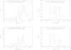 |
Fig. 11 Top left: observed core-separation distribution (solid line) compared with the expected distribution for random distribution of the same number of cores as the observed sample over an identical area (dashed line). Top right: same as in the top left panel but for the nearest-neighbour distribution. Bottom panels: same as in the top panels, but SMM 7, IRAS 05412-0105, and IRAS 05413-0104 have been excluded from the samples. |
Statistics of the core spatial distributions in Orion B9.
5.9. The lifetime and origin of dense cores in Orion B9
According to the scenario of turbulence-regulated star formation, the prestellar core evolution is dynamic and the corresponding lifetime is only a few times the free-fall time (Mac Low & Klessen 2004; Vázquez-Semadeni et al. 2005). Several results of our study conform to this scenario: as was discussed in Sect. 5.2, the Orion B9 cores could have been formed in turbulent shocks where the dissipation of the kinetic energy of turbulent motions took place. It was also concluded that the timescale for core formation should be comparable to the free-fall time. On the other hand, the abundances of the N-bearing species studied in the present paper are consistent with those predicted by chemical models based on dynamical prestellar core evolution (Sect. 5.6). Moreover, in Paper I we deduced that there are equal numbers of pre- and protostellar cores in the Orion B9 region, which suggest that the corresponding lifetimes are comparable. Based on similar statistical results, i.e., Npre/Nproto ≈ 1, recent studies have shown that the duration of the prestellar phase of core evolution at densities n(H2) ≳ 104 cm-3 is only a few times the free-fall time (see references in Paper I; Evans et al. 2009). It is possible that some of the cores do not belong to the same volume of the cloud as those with centroid velocities around 9 km s-1. Even if the cores with lower centroid velocities are excluded (i.e., SMM 7, and IRAS 05413-0104 and 05412-0105), the above ratio is 5:4 = 1.25, which is still consistent with the dynamic core evolution scenario.
In the present study (and in Paper I), we found that the CMFs in Orion B9 and Orion B North very likely represent the subsamples of the same parent distribution, and resemble the stellar IMF (Nutter & Ward-Thompson 2007). Numerical simulations of turbulent fragmentation have been able to reproduce the general shape of the IMF (e.g., Padoan & Nordlund 2002; Ballesteros-Paredes et al. 2006). On the other hand, recent models concerning fragmentation initiated by the ambipolar diffusion (AD) have likewise succeeded in explaining the connection between the CMF and the IMF (Kunz & Mouschovias 2009).
In Paper I, we used the spatial distribution of cores, which seemed to mimic a random distribution, as an argument for the dominance of turbulent fragmentation in core formation. Moreover, we stated that because region represents clustered star formation, the turbulence is most likely driven on large scales (e.g., Klessen et al. 2000; Klessen 2001). However, the present molecular line data and a more careful analysis of the spatial distribution have called both arguments into question: According to the K-S test, the core distribution is unlikely to be random, and the core properties resemble closely those in the regions of isolated star formation.
To summarise, the current data suggest that the evolution of the Orion B9 cores is dynamic. As discussed in Sect. 5.7, the Orion B9 region is likely to be influenced by the massive stars of the Ori OB 1b group. This interaction process could have led to the driving of the large-scale turbulence and/or to the compression of the cloud material into dense sheets and filaments as observed in molecular clouds. These structures could have then been fragmented into dense cores via gravitational instability as suggested by the Jeans-length analysis in Sect. 5.8. Further investigations of the chemistry, deuteration, and the degree of ionisation can help to fix the evolutionary timescales, and thereby estimate the roles of turbulence, thermo-gravitational instability, and ambipolar diffusion in the core formation.
6. Summary and conclusions
We observed the NH3(1,1) and (2,2) inversion transitions, and the N2H+(3−2) lines towards the submm cores in Orion B9 star-forming region with the Effelsberg 100-m and APEX telescopes, respectively. These line observations were combined with our previous 870 μm submm dust continuum data of the region. The data were used to determine the physical characteristics of dense cores in this region. We mainly investigated the temperatures and kinematics of the cores, and recalculated the temperature-dependent quantities presented in Paper I (Miettinen et al. 2009). Our main results and conclusions are as follows:
-
1.
The gas kinetic temperatures of the cores are in the range ~9.4−13.9 K, with an average value of about 12 K. No significant difference in Tkin was found between starless and protostellar cores. The temperature values are similar to those in nearby low-mass star-forming regions.
-
2.
The cores are characterised by subsonic, or at most transonic, non-thermal motions. Thus, the cores are kinematically similar to those in nearby low-mass star-forming regions.
-
3.
In the case of protostellar cores, we found a positive correlation between the non-thermal NH3 linewidth and bolometric luminosity. This can be understood so that on one hand, the embedded central protostar enhances the level of turbulent motions within the parent core, and on the other hand, more turbulent initial conditions lead to the formation of more massive stars with higher luminosity.
-
4.
The core masses are, on average, about 11% higher than those reported in Paper I when calculated by assuming that Tdust = Tkin (in Paper I, we assumed that Tdust = 10 K for starless cores). These masses are very likely drawn from the same parent distribution as the core masses in the northern part of Orion B (Nutter & Ward-Thompson 2007).
-
5.
Almost all cores were found to be close to virial equilibrium when the internal kinetic pressure and self-gravity are taken into account. In addition, they are likely to be exposed to a substantial turbulent ram pressure from the intercore gas (as can be evaluated from previous 13CO data), which is sufficient to bring them to equilibrium or make them collapse. In particular, it seems probable that most if not all starless cores detected in this survey are prestellar.
-
6.
The fractional NH3 and N2H+ abundances in the cores are ~1.5−9.8 × 10⁻⁸ and ~0.2−5.9 × 10⁻¹⁰, respectively. The NH3/N2H+ column density ratio is higher in prestellar cores than protostellar cores. Similar trend has also been observed in other star-forming regions. The NH3 abundance appears to decrease with increasing gas density (as traced by 870 μm continuum emission). This tendency is likely to be caused by the accretion of NH3 onto grains at very high densities, and conforms to the recent results of Friesen et al. (2009) in Ophiuchus.
-
7.
A few cores have a much lower radial velocity compared to the systemic velocity of the region (~9 km s-1), and do not necessarily belong to the same volume of the cloud as the rest of the cores. Instead, they are likely to be members of the “low-velocity” part of Orion B. This increases the relative number of pre- and protostellar cores in Orion B9 and consequently, the statistical lifetime of the prestellar phase of core evolution (by 25% in both cases).
-
8.
Many of the properties of dense cores in Orion B9 suggest that their evolution is likely to be dynamic, i.e., comparable to the free-fall timescale. On the other hand, the new data and an improved analysis of spatial distribution have made the role of turbulent fragmentation in the core formation less evident than it appeared in Paper I. According to the new results, the cores are unlikely to be randomly positioned within the region, and they are not clustered in the way expected if the fragmentation is driven on large scale turbulence. Futhermore, the core properties are similar to those found in the regions of isolated star formation.
-
9.
The Orion B9 region is likely to be influenced by the massive stars of the nearby Ori OB 1b group. This explains the origin of the low-velocity material in the southern parts of Orion B (Wilson et al. 2005). Moreover, this interaction process could have led to formation of dense filaments, from which the dense cores were fragmented out by the action of gravitational instability.
Acknowledgments
We thank the referee for helpful comments, and the staff at the Effelsberg for their hospitality and support during our observations. We also thank the staff at the APEX telescope for performing the observations in the service mode. The authors acknowledge support from the Academy of Finland through grants 117206 and 132291.
References
- Aikawa, Y., Herbst, E., Roberts, H., & Caselli, P. 2005, ApJ, 620, 330 [NASA ADS] [CrossRef] [Google Scholar]
- Aikawa, Y., Wakelam, V., Garrod, R. T., & Herbst, E. 2008, ApJ, 674, 984 [NASA ADS] [CrossRef] [Google Scholar]
- Aoyama, H., Mizuno, N., Yamamoto, H., et al. 2001, PASJ, 53, 1053 [NASA ADS] [Google Scholar]
- Ballesteros-Paredes, J., Gazol, A., Kim, J., et al. 2006, ApJ, 637, 384 [NASA ADS] [CrossRef] [Google Scholar]
- Bally, J. 2008, Handbook of Star Forming Regions, I, 459 [NASA ADS] [Google Scholar]
- Bally, J., Reipurth, B., & Aspin, C. 2002, ApJ, 574, L79 [NASA ADS] [CrossRef] [Google Scholar]
- Bertoldi, F., & McKee, C. F. 1992, ApJ, 395, 140 [NASA ADS] [CrossRef] [Google Scholar]
- Boulares, A., & Cox, D. P. 1990, ApJ, 365, 544 [NASA ADS] [CrossRef] [Google Scholar]
- Buckle, J. V., Curtis, E. I., Roberts, J. F., et al. 2010, MNRAS, 401, 204 [NASA ADS] [CrossRef] [Google Scholar]
- Busquet, G., Palau, A., Estalella, R., et al. 2009, A&A, 506, 1183 [NASA ADS] [CrossRef] [EDP Sciences] [Google Scholar]
- Caselli, P., & Myers, P. C. 1995, ApJ, 446, 665 [NASA ADS] [CrossRef] [Google Scholar]
- Caselli, P., Benson, P. J., Myers, P. C., & Tafalla, M. 2002, ApJ, 572, 238 [NASA ADS] [CrossRef] [Google Scholar]
- Caselli, P., Vastel, C., Ceccarelli, C., et al. 2008, A&A, 492, 703 [NASA ADS] [CrossRef] [EDP Sciences] [Google Scholar]
- Evans, N. J., Dunham, M. M., Jørgensen, J. K., et al. 2009, ApJS, 181, 321 [NASA ADS] [CrossRef] [Google Scholar]
- Flower, D. R., Pineau des Forêts, G., & Walmsley, C. M. 2006, A&A, 456, 215 [NASA ADS] [CrossRef] [EDP Sciences] [Google Scholar]
- Foster, J. B., Rosolowsky, E. W., Kauffmann, J., et al. 2009, ApJ, 696, 298 [NASA ADS] [CrossRef] [Google Scholar]
- Friesen, R. K., di Francesco, J., Shirley, Y. L., & Myers, P. C. 2009, ApJ, 697, 1457 [NASA ADS] [CrossRef] [Google Scholar]
- Friesen, R. K., di Francesco, J., Shimajiri, Y., & Takakuwa, S. 2010, ApJ, 708, 1002 [NASA ADS] [CrossRef] [Google Scholar]
- Frieswijk, W. W. F., Spaans, M., Shipman, R. F., Teyssier, D., & Hily-Blant, P. 2007, A&A, 475, 263 [NASA ADS] [CrossRef] [EDP Sciences] [Google Scholar]
- Goldsmith, P. F., & Langer, W. D. 1978, ApJ, 222, 881 [NASA ADS] [CrossRef] [Google Scholar]
- Harju, J., Walmsley, C. M., & Wouterloot, J. G. A. 1993, A&AS, 98, 51 [Google Scholar]
- Harju, J., Haikala, L. K., Lehtinen, K., et al. 2006, A&A, 454, L55 [NASA ADS] [CrossRef] [EDP Sciences] [Google Scholar]
- Ho, P. T. P., & Townes, C. H. 1983, ARA&A, 21, 239 [NASA ADS] [CrossRef] [Google Scholar]
- Ho, P. T. P., Barrett, A. H., Myers, P. C., et al. 1979, ApJ, 234, 912 [NASA ADS] [CrossRef] [Google Scholar]
- Hotzel, S., Harju, J., Lemke, D., Mattila, K., & Walmsley, C. M. 2001, A&A, 372, 302 [NASA ADS] [CrossRef] [EDP Sciences] [Google Scholar]
- Ikeda, N., Kitamura, Y., & Sunada, K. 2009, ApJ, 691, 1560 [NASA ADS] [CrossRef] [Google Scholar]
- Jijina, J., Myers, P. C., & Adams, F. C. 1999, ApJS, 125, 161 [NASA ADS] [CrossRef] [Google Scholar]
- Johnstone, D., Fich, M., Mitchell, G. F., & Moriarty-Schieven, G. 2001, ApJ, 559, 307 [NASA ADS] [CrossRef] [Google Scholar]
- Johnstone, D., Matthews, H., & Mitchell, G. F. 2006, ApJ, 639, 259 [NASA ADS] [CrossRef] [Google Scholar]
- Johnstone, D., Rosolowsky, E., Tafalla, M., & Kirk, H. 2010, ApJ, 711, 655 [NASA ADS] [CrossRef] [Google Scholar]
- Kauffmann, J., Bertoldi, F., Bourke, T. L., et al. 2008, A&A, 487, 993 [NASA ADS] [CrossRef] [EDP Sciences] [Google Scholar]
- Kirk, H., Johnstone, D., & Tafalla, M. 2007, ApJ, 668, 1042 [NASA ADS] [CrossRef] [Google Scholar]
- Klein, B., Philipp, S. D., Krämer, I., et al. 2006, A&A, 454, L29 [NASA ADS] [CrossRef] [EDP Sciences] [Google Scholar]
- Klessen, R. S. 2001, ApJ, 556, 837 [Google Scholar]
- Klessen, R. S., Heitsch, F., & Mac Low, M.-M. 2000, ApJ, 535, 887 [NASA ADS] [CrossRef] [Google Scholar]
- Kunz, M. W., & Mouschovias, T. C. 2009, MNRAS, 399, L94 [NASA ADS] [Google Scholar]
- Lada, C. J., Muench, A. A., Rathborne, J., et al. 2008, ApJ, 672, 410 [NASA ADS] [CrossRef] [Google Scholar]
- Larson, R. B. 1981, MNRAS, 194, 809 [NASA ADS] [CrossRef] [Google Scholar]
- Lee, C.-F., Ho, P. T. P., Bourke, T. L., et al. 2008, ApJ, 685, 1026 [NASA ADS] [CrossRef] [Google Scholar]
- Mac Low, M.-M., & Klessen, R. S. 2004, Rev. Mod. Phys., 76, 125 [NASA ADS] [CrossRef] [Google Scholar]
- Maruta, H., Nakamura, F., Nishi, R., Ikeda, N., & Kitamura, Y. 2010, ApJ, 714, 680 [NASA ADS] [CrossRef] [Google Scholar]
- Miettinen, O., Harju, J., Haikala, L. K., et al. 2009, A&A, 500, 845 (Paper I) [NASA ADS] [CrossRef] [EDP Sciences] [Google Scholar]
- Myers, P. C., & Benson, P. J. 1983, ApJ, 266, 309 [NASA ADS] [CrossRef] [Google Scholar]
- Myers, P. C., Ladd, E. F., & Fuller, G. A. 1991, ApJ, 372, L95 [NASA ADS] [CrossRef] [Google Scholar]
- Nutter, D., & Ward-Thompson, D. 2007, MNRAS, 374, 1413 [NASA ADS] [CrossRef] [Google Scholar]
- Ott, M., Witzel, A., Quirrenbach, A., et al. 1994, A&A, 284, 331 [NASA ADS] [Google Scholar]
- Padoan, P., & Nordlund, Å. 2002, ApJ, 576, 870 [Google Scholar]
- Pagani, L., Daniel, F., & Dubernet, M.-L. 2009, A&A, 494, 719 [NASA ADS] [CrossRef] [EDP Sciences] [Google Scholar]
- Peng, B., Kraus, A., Krichbaum, T. P., & Witzel, A. 2000, A&AS, 145, 1 [Google Scholar]
- Pillai, T., Wyrowski, F., Carey, S. J., & Menten, K. M. 2006, A&A, 450, 569 [NASA ADS] [CrossRef] [EDP Sciences] [Google Scholar]
- Rosolowsky, E. W., Pineda, J. E., Foster, J. B., et al. 2008, ApJS, 175, 509 [NASA ADS] [CrossRef] [Google Scholar]
- Schnee, S., Rosolowsky, E., Foster, J., et al. 2009, ApJ, 691, 1754 [NASA ADS] [CrossRef] [Google Scholar]
- Shetty, R., Kauffmann, J., Schnee, S., Goodman, A. A., & Ercolano, B. 2009, ApJ, 696, 2234 [NASA ADS] [CrossRef] [Google Scholar]
- Tafalla, M., Myers, P. C., Caselli, P., Walmsley, C. M., & Comito, C. 2002, ApJ, 569, 815 [NASA ADS] [CrossRef] [Google Scholar]
- Tafalla, M., Myers, P. C., Caselli, P., & Walmsley, C. M. 2004, A&A, 416, 191 [NASA ADS] [CrossRef] [EDP Sciences] [Google Scholar]
- Tafalla, M., Santiago-García, J., Myers, P. C., et al. 2006, A&A, 455, 577 [NASA ADS] [CrossRef] [EDP Sciences] [Google Scholar]
- Vassilev, V., Meledin, D., Lapkin, I., et al. 2008, A&A, 490, 1157 [NASA ADS] [CrossRef] [EDP Sciences] [Google Scholar]
- Vázquez-Semadeni, E., Kim, J., Shadmehri, M., & Ballesteros-Paredes, J. 2005, ApJ, 618, 344 [NASA ADS] [CrossRef] [Google Scholar]
- Wilson, B. A., Dame, T. M., Masheder, M. R. W., & Thaddeus, P. 2005, A&A, 430, 523 [NASA ADS] [CrossRef] [EDP Sciences] [Google Scholar]
- Wiseman, J., Wootten, A., Zinnecker, H., & McCaughrean, M. 2001, ApJ, 550, L87 [NASA ADS] [CrossRef] [Google Scholar]
All Tables
All Figures
|
Fig. 1 NH3(1,1) and (2,2) spectra measured from the pre- and protostellar cores in Orion B9. The temperature scale is in TMB. NH3(2,2) spectra are offset by –1 K from zero baseline for clarity. Note that there are two velocity components towards SMM 4 and Ori B9 N, and that no lines were detected towards IRAS 05412-0105. |
| In the text | |
|
Fig. 2 NH3(1,1) spectrum measured from SMM 6 using the FFTS
with a 20 MHz bandwidth. Below the spectrum are shown the model fit to the
hyperfine structure and the residual spectrum. Satellite hyperfine components in
the |
| In the text | |
|
Fig. 3 N2H+(3−2) spectra measured from the pre- and protostellar cores in Orion B9. Spectra are overlaid with the 38 component hyperfine structure fits. Hyperfine fits to the second velocity components are indicated by red lines. Note that only the second velocity component is detected towards SMM 4. The relative velocity of each individual hyperfine component is labelled with a short bar on the spectrum towards IRAS 05399-0121 (top left panel). The temperature scale is in TMB. |
| In the text | |
|
Fig. 4 Top: the centroid velocity of the N2H+(3−2) emission versus the velocity of the NH3(1,1) emission. Bottom: Log-log plot of the N2H+(3−2) linewidth versus the NH3(1,1) linewidth. Prestellar cores are indicated by open diamonds and protostellar cores are marked by filled diamonds. In both plots, the dashed line shows the equality. |
| In the text | |
|
Fig. 5 Non-thermal versus thermal (for H2, i.e., the isothermal sound speed) linewidths in log-log scales. The dashed line indicates ΔvNT = ΔvT. The dotted and dash-dotted lines show relationships found by 4 for NH3 cores with and without cluster association, respectively. Symbols have the same meaning as in Fig. 4. |
| In the text | |
|
Fig. 6 Linewidth versus radius for the cores in Orion B9 in log-log scales. The 5 relation is shown by the dotted line. The dashed line indicates the relation derived by Ikeda et al. (2009) for the H13CO+ cores in Orion B. Symbols have the same meaning as in Fig. 4. |
| In the text | |
|
Fig. 7 Left: total internal kinetic gas pressure versus core mass. Right: the ratio of thermal to non-thermal pressure as a function of mass. The dashed horizontal line marks the point at which thermal and non-thermal pressure support are equal. Both plots are in log-log scales, and the symbols have the same meaning as in Fig. 4. |
| In the text | |
|
Fig. 8 Left: virial parameter versus core mass. The dashed line indicates the virial equilibrium limit (αvir = 1), and the dash-dotted line shows the limit of gravitational boundedness (αvir = 2). Right: ratio of 3D velocity dispersion to escape velocity against core mass. The dashed line indicates σ3D/vesc = 1. All cores are likely to be gravitationally bound. The solid line in both plots indicates the least-squares fit to the data. Both plots are in log-log scales, and the symbol key is identical to that of Fig. 4. |
| In the text | |
|
Fig. 9 Left: Tkin versus Tbol. The dashed line indicates Tkin = Tbol. Right: ΔvNT versus Lbol. The solid line indicates the least-squares fit to the data. The upper and lower dashed lines represent relationships found by 4 for NH3 cores with and without cluster association, respectively. The dash-dotted line shows the relationships found by Myers et al. (1991) for IRAS point sources. Both plots are in log-log scales. |
| In the text | |
|
Fig. 10 Comparison of chemical abundances as a function of H2 column and number density. All plots are in log-log scales, and the symbol key is identical to that of Fig. 4. The solid lines indicate the least-squares fits to the data. Left: x(NH3) versus N(H2). The dashed line indicates the relationship found by Friesen et al. (2009, 2010) for Oph B2. Middle: x(NH3) versus n(H2). Right: NH3/N2H+ column density ratio versus N(H2). |
| In the text | |
|
Fig. 11 Top left: observed core-separation distribution (solid line) compared with the expected distribution for random distribution of the same number of cores as the observed sample over an identical area (dashed line). Top right: same as in the top left panel but for the nearest-neighbour distribution. Bottom panels: same as in the top panels, but SMM 7, IRAS 05412-0105, and IRAS 05413-0104 have been excluded from the samples. |
| In the text | |
Current usage metrics show cumulative count of Article Views (full-text article views including HTML views, PDF and ePub downloads, according to the available data) and Abstracts Views on Vision4Press platform.
Data correspond to usage on the plateform after 2015. The current usage metrics is available 48-96 hours after online publication and is updated daily on week days.
Initial download of the metrics may take a while.