| Issue |
A&A
Volume 522, November 2010
|
|
|---|---|---|
| Article Number | A106 | |
| Number of page(s) | 19 | |
| Section | Interstellar and circumstellar matter | |
| DOI | https://doi.org/10.1051/0004-6361/201014524 | |
| Published online | 09 November 2010 | |
Star formation in Cometary Globule 1: the second generation⋆,⋆⋆
1
Observatory, University of Helsinki,
Finland
2
Department of Physics, Division of Geophysics and
Astronomy, PO Box
64, 00014 University of
Helsinki, Finland
e-mail: lauri.haikala@helsinki.fi
3
South African Astronomical Observatory,
PO Box 9, Observatory
7935, Cape Town, South
Africa
4
Southern African Large Telescope Foundation, PO Box
9, Observatory, 7935, Cape
Town, South Africa
Received: 28 March 2010
Accepted: 9 July 2010
Context. Cometary Globule 1 (CG 1) is the archetype Cometary Globule in the Gum nebula.
Aims. We attempt to discover stars possibly embedded in the globule head of the Gum nebula and to map distribution of its ISM.
Methods. We analyse C18O spectral line observations, NIR spectrosopy, narrow and broad band NIR imaging, and stellar photometry to determine the structure of the CG 1 head and the extinction of stars in its direction.
Results. A young stellar object (YSO) associated with a bright NIR nebulosity and a molecular hydrogen object (MHO 1411, a probable obscured HH-object) were discovered in the globule. Molecular hydrogen and Brγ line emission is seen in the direction of the YSO. The observed maximum optical extinction in the globule head is 9.m2. The peak N(H2) column density and the total mass derived from the extinction are 9.0 × 1021 cm-2 and 16.7 M⊙ (d/300 pc)2. The C18O emission in the globule head is detected in a 15 by 4′ area with a sharp maximum SW of the YSO. Three regions can be discerned in C18O line velocity and excitation temperature. Because of variations in the C18O excitation temperature the integrated C18O line emission does not follow the optical extinction. It is argued that the changes in the C18Oexcitation temperatures are caused by radiative heating by NX Pup and interaction of the YSO with the parent cloud. No indication of a strong molecular outflow from the YSO is evident in the molecular line data. The IRAS point source 07178–4429 located in the CG 1 head resolves into two sources in the HIRES enhanced IRAS images. The 12 and 25 μm emission originates mainly in the star NX Puppis and the 60 and 100 μm emission in the YSO.
Key words: stars: formation / stars: pre-main sequence / dust, extinction / ISM: clouds / Herbig-Haro objects / infrared: stars
Based partly on observations collected at the European Southern Observatory, La Silla, Chile and partly obtained from the ESO/ST-ECF Science Archive Facility.
Appendices A, B and C are only available in electronic form at http://www.aanda.org
© ESO, 2010
1. Introduction
Sanduleak (1974) noted a 5′ by 10′ dark cloud west of the emission-line star Hen 32 (CoD –44 3318, NX Pup). This dark cloud was later included in a list of cometary globules by Hawarden & Brand (1976). Cometary globules are elongated dark clouds with compact, dusty “heads” and long faintly luminous “tails”. The first list contained 12 sources of which ten were in the outskirts of the Gum nebula. The sizes vary from few arcminutes (e.g. CG 5) to tens of arcminutes (CG 12). Since their discovery similar cometary structures have been found to be common among interstellar clouds, the scales ranging from isolated tiny globules to complete cometary shaped star-forming regions such as the Corona Australis cloud. It has been suggested that the formation of the classical CGs is caused by radiation-driven implosion (Reipurth 1983) of an isolated, extended globule or a passage of a supernova plane blast wave colliding with an extended globule (Brand et al. 1983).
CG 1 (Hawarden & Brand 1976) is a prototypical Cometary Globule. It has a few arcminute sized compact bright rimmed head and nearly a half-a-degree-long tail. The bright pre-main-sequence binary star NX Pup lies just outside the opaque globule head. The IRAS point source 07178–4429 lies between NX Pup and the opaque globule head. It has far infrared (FIR) colours similar to young stellar objects. Extensive molecular line observations of CG 1 are presented in Harju et al. (1990) (hereafter HSHWSP). Even though HSHWSP report rather strong 12CO lines (SEST antenna temperatures up to 10 K), the C18O(1–0) emission is weak. In the C18Omaximum located in the globule head, the integrated C18O(1–0) main-beam brightness temperature (TMB) was less than 0.55 K km s-1. Two 12CO velocity components are seen in the globule head. The stronger one follows the globule optical image from head to tail. The weaker velocity component is distributed in an elongated structure and coincides with the bright “nose”-like extension in optical surface emission, which extends to below the star NX Pup. The Bourke et al. (1995) single point ammonia observation in the CG 1 head was a non-detection. Single point observations of IRAS 07178–4429 in CO(3–2), C18O(3–2), HCO+ (4–3), and H13CO+ (4–3) are presented in van Kempen et al. (2009). The authors conclude that the point source has no associated HCO+ core and that it very likely does not have a circumstellar shell.
The distance to CG 1 is uncertain and the estimates range from 300 pc (Franco 1990) to 500pc (Brand et al. 1983). Franco (1990) analysed the distribution of stellar E(b–y) colour excesses in the direction of the Gum nebula and concluded that the distance to the centre of the nebula is 290 ± 30 pc. The Brand et al. (1983) distance relies on NIR photometry of the variable star NX Pup, which lies near the globule head. In accordance with the Franco (1990) result, HSHWSP adopted 300 pc as the distance to CG 1. This paper will also use the 300 pc.
It has been suggested that the Herbig AeBe star NX Pup was formed in the globule (e.g., Brand et al. 1983; Reipurth 1983). The star is a close visual binary (Bernacca et al. 1993) and a further T Tau star located 7″ away was discovered by Brandner et al. (1995). The globule head is strongly obscured in the optical and in the 2MASS survey the number of stars in the globule head is also smaller than in the surroundings. A deeper-than-2MASS near-infrared (NIR) study is therefore needed to study the possible stellar population still embedded in the globule and the distribution of dust and gas in the globule head. We present J, H, and Ks NIR imaging of the CG 1 head with the InfraRed Survey Facility (IRSF) 1.4 m telescope at the South African Astronomical Observatory SAAO and the 3.5 m New Technology Telescope (NTT) at La Silla. Low resolution NIR spectroscopy and narrow band imaging in the H2 1–0 S(1) 2.12 μm line were also conducted with the NTT. The C18O(1–0) and (2–1) molecular line observations of the globule head were obtained at the Swedish ESO Submillimetre Telescope (SEST) at La Silla. Observations, data reduction, and calibration procedures are described in Sect. 2 and the observational results in Sect. 3. The new results are discussed and compared with available data at other wavelengths in Sect. 4. The results are summarised and the conclusions drawn in Sect. 5.
2. Observations and data reduction
2.1. NIR imaging
The head of CG 1 was imaged in J, H, and Ks with the Simultaneous InfraRed Imager for Unbiased Survey (SIRIUS, Nagayama et al. 2003) on the IRSF 1.4 m telescope on Jan. 2007. The three colours were observed simultaneously. The SIRIUS field of view is 77 × 77 and the pixel scale 0453. The observations were hampered by high humidity and the average seeing was worse than 1″. The observations were carried out in the on-off mode instead of the standard jitter mode to preserve the surface brightness. After each on-integration of 10 s, an off-position outside the globule was observed with the same integration time. Jittering was performed after each on-off pair. Sky flats were observed every evening and morning.
The Son of Isaac (SOFI) imaging in Js, H, and Ks at NTT was performed in Feb. 2007. The SOFI field of view is 49 and the pixel size 0288. The observing was done in the standard jittering mode in observing blocks of approximately 1 h. The integrations consisted of 6 individual 10 s integrations and the observed total on-source time was 1.5 h in each filter. The average seeing was ~07. The bright pre-main-sequence star NX Pup, which is located to the east of the globule head, was not within the field of view. A reference position at the same Galactic latitude but outside the globule (7h18m –44o05′, J2000) was observed in all colours. Standard stars from the Persson et al. (1998) faint NIR standard list were observed frequently during the nights.
Extended molecular hydrogen emission was searched for by imaging the CG 1 head with the narrow SOFI filters NB H2 S1 (H2 1–0 S(1), 2.12 μm) and NB 2.090 (continuum). The narrow-band imaging was done in the standard jittering mode.
The IRAF1 external XDIMSUM package was used to reduce the SIRIUS and SOFI imaging data. The images were examined for cosmic-ray hits and then sky-subtracted. The two nearest images in time to each image were used in the sky subtraction. An object mask was constructed for each image. Applying these masks in the sky subtraction produced hole masks for each sky-subtracted image. Special dome flats and illumination correction frames provided by the NTT team were used to flat field and illumination-correct the sky-subtracted SOFI images. Sky flats were used to flat-field the SIRIUS images. Rejection masks combined from a bad pixel mask and individual cosmic ray and hole masks were used when averaging the registered images. The reduced SOFI Js, H, and Ks images are shown in Figs. A.1, A.2, and A.3.
NX Pup is very bright and produces an artifact (inter-quadrant row cross talk) which appears as a stripe in the same column as the star and symmetrically on the other half of the detector in the SIRIUS images. Reflections in the SIRIUS filters cause ring-like ghosts around NX Pup. We attempted to correct for neither the inter-quadrant row cross talk nor the reflections.
The SExtractor software v 2.5.0 (Bertin & Arnouts 1996) package was used to obtain stellar photometry of the reduced SOFI images. The galaxies were excluded using the SExtractor CLASS keyword and by visually inspecting the images. After elimination of the non-stellar sources, 262 stars remained. The magnitude zero points of the summed data were fixed using the standard star measurements. The instrumental magnitudes were first converted to the Persson et al. (1998) photometric system and then to the 2MASS photometric system as described in Ascenso et al. (2007). The magnitude scale was checked by comparing the SOFI photometry of stars in common with 2MASS that have high quality 2MASS photometry. The limiting magnitudes are approximately 21.m5, 20.m5, and 20.m5 for J, H, and Ks, respectively. The limiting magnitude however varies over the observed area and is brighter in the regions where the background surface brightness is strong.
2.2. NIR spectroscopy
A low resolution SOFI spectrum was acquired covering the wavelengths from 1.53 μm to 2.52 μm (resolving power 980) using a slit oriented along a bright surface brightness feature (see Figs. 3 and 4). The SOFI standard nodding observing template was used. La Silla observatory IR standard F7V star Hip37123 was observed as a telluric standard.
The spectroscopic science frames were flatfielded using ON-OFF flats, illumination and cosmic-ray corrected, and then subtracted pairwise from each other. Xe-arcs were used to fit the wavelength solution and correct for the two dimensional shape distortion. Frames were then shifted, coadded, and traced. The standard star was reduced in exactly the same way, and its one dimensional extracted spectrum was divided into the two dimensional target per row, and the result multiplied by a smooth black-body model of the star, thereby removing telluric features and also performing a relative flux calibration.
2.3. C18O mapping
The C18O(1–0) and (2–1) molecular line observations were made in Sep. 2000 at SEST. The observations were conducted with the SEST 3 and 1 mm (IRAM) dual SiS SSB receiver using the frequency-switching observing mode. A 6 MHz and 18 MHz frequency switch was used at the C18O (1–0) and (2–1) line frequencies, respectively. The CG1 globule head was mapped simultaneously in the C18O (1–0) and the C18O (2–1) transitions in a regular grid with a spacing of 20″. Altogether 137 positions were observed using one-minute integration times. Selected positions were integrated longer. Typical values of the effective SSB system temperatures outside the atmosphere ranged from 170 K to 250 K. The SEST high-resolution 2000-channel acousto-optical spectrometer (bandwidth 86 MHz, channel width 43 kHz) was divided into two to measure the two receivers simultaneously. At the observed frequencies, 109.782173 GHz and 219.560353 GHz, the spectrometer channel width corresponds to ~0.12 km s-1 and ~0.06 km s-1, respectively. The SEST HPBW and main-beam efficiency were 47″ and 0.7, respectively, for the C18O(1–0) frequency, and 23″ and 0.5 for the C18O(2–1) frequency. Calibration was performed using the chopper wheel method. Pointing was checked regularly towards SiO maser sources and the pointing accuracy is estimated to be better than 5″.
The frequency-switched spectra were first folded and a second order baseline was then subtracted. The observed spectrum rms was typically ~0.14 K and ~0.2 K in the TMB scale for the C18O(1–0) and (2–1) transitions, respectively. All the SEST line temperatures in this paper are in the TMB units, i.e., corrected to outside the atmosphere, assuming that the source fills the main beam.
3. Results
3.1. JHKs imaging
False colour SIRIUS and SOFI images of the CG 1 head are shown in Figs. 1 and 2, respectively. The J, H, and Ks bands are coded in blue, green, and red, respectively. The SOFI image contains only the obscured globule head, whereas the SIRIUS image also contains the bright pre-main-sequence star NX Pup and a bright reflection nebulosity south of it. The SIRIUS observations were made in the on-off mode, which conserves the extended surface brightness. The SOFI observations were obtained in the jitter mode where the surface brightness with scale larger than the jitter box (30″ in this case) is smeared and/or cancelled in the data reduction. Only small-size features and gradients in the original surface brightness structure are retained. Point-like sources and galaxies are unaffected.
The edges of the globule are well defined in both the SIRIUS and the SOFI images. In the SIRIUS image, the surface brightness is extended NW of NX Pup and a narrow filament follows the globule southern edge. The surface of the CG 1 head is covered with narrow, faint filaments in the SOFI image. Because of the jittering observing mode, the extended surface brightness is transformed into filaments that trace small-scale gradients in the actual surface brightness.
Besides the stars and numerous galaxies, a semistellar source surrounded by a bright nebulosity is seen in both the SIRIUS and SOFI images. The nebulous source has the appearance of a typical young stellar source (see e.g. Zinnecker et al. 1999) and is referred to as YSO in the following. A bright and elongated surface brightness feature protrudes SE of the YSO in the Ks image. This feature is referred as the YSO_SE filament in the following. Thin, wispy filaments extend both west and east of the YSO in Fig. 2. The nebulosity associated with the YSO is extended and very bright. Therefore, it had to be masked heavily in the jitter sky frames during the data reduction. As a consequence, most of the structure seen in the reduced images around the YSO is real and not smeared like the other extended structures in the SOFI images. A faint surface brightness patch is seen in the SOFI images ~90″ west of the YSO. Both the thin filaments and the surface brightness patch west of the YSO are seen in all three colours. Except for the YSO and the regions NW and SE of it the globule NIR surface brightness is predominantly blue in Fig. 2, i.e. more pronounced in the Js band than in the two other colours. The ring-segment-like structure facing the bright star NX Pup seen in Figs. 1 and 2 as well as the bright patch south of this star (Fig. 1) have counterparts in the optical images of CG 1 (see e.g. Brand et al. 1983, Plate 1). The YSO and these features are identified in Fig. 3. The ring-segment-like structure and the brightest thin filaments are indicated by a continuous line and dashed lines, respectively. The YSO_SE filament is marked with a line in the insert and the nebulous patch west of the YSO with a circle.
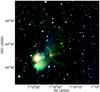 |
Fig. 1 Colour–coded SIRIUS image of the CG 1 head. The J, H, and Ks bands are coded in blue, green, and red, respectively. Square root scaling has been used to enhance the faint surface brightness structures. NX Pup is the brightest star in the image at 7h19m283, − 44o35′103. |
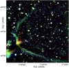 |
Fig. 2 Colour–coded SOFI image of CG 1 head. The Js, H, and Ks bands are coded in blue, green, and red, respectively. Square root scaling has been used to enhance the faint surface brightness structures. |
A zoomed image of the YSO in the SOFI image in three colours is shown in the three lower panels of Fig. 4. The filter is indicated in the upper left corner of each panel. The size of the lower panels is 46″ by 46″, which approximately corresponds to the SEST HPBW at the C18O(1–0) line frequency, 109 GHz. The upper 23″ by 23″ panels (SEST HPBW at the C18O(2–1) frequency, 219 GHz) show surface brightness contours superimposed on Gaussian smoothed images. The contour levels and the grey scale were chosen to enhance the contrast in surface brightness for each filter. The line in the Ks image shows the orientation of the spectrometer slit. The cross in all the panels indicates the position of the semi-stellar source in the Ks image. The H and Ks surface brightness contours are overlaid on a 23″ by 23″ Js grey scale image in Fig. A.4. The absolute surface brightness in the Js image is very low compared with that in the Ks image. The Ks semi-stellar source lies behind a narrow obscuring lane in the Js image. In the H filter, the maximum emission lies east of the Ks maximum and is not stellar like. The half width of the Ks semi-stellar source intensity profile in the EW direction is nearly twice that of isolated stars elsewhere in the image. This indicates that even at the Ks maximum, a large part of the observed emission is reflected light and not direct light from the central source.
The YSO is visible in the 2MASS survey (2MASS 07192185-4434551), which is a Ks band detection (13.m42) only. The 2MASS extended source 2MASX J07192176-4434591 corresponds to the extended YSO nebulosity. The YSO is also visible in the Ks image presented in Santos et al. (1998), who identify it as a red object, possibly a YSO in an early evolutionary stage embedded in the globule.
3.2. NIR spectroscopy
Part of the SOFI low-resolution long-slit spectrum, in both two dimensional and extracted format, is shown in Fig. 5. The 12″ centre part of the spectrum through the YSO nebulosity and the YSO SE_filament is shown in Fig. 5, lower panel. Extracted continuum- subtracted spectrum convolved with a 3-pixel box-car is shown in the upper panel. The wavelengths of the H2 lines within the displayed spectral region and of the Brγ line are indicated. The spectrum has been normalized for an (1–0) S(1) intensity of unity.
At least three H2 lines and the Brγ line are evident in the spectrum. The H2 lines are detected in the centre of the nebulosity and also at the base of the bright YSO_SE filament. The filament is most clearly seen in the H2 1–0 (S1) transition. The Brγ emission is strictly constrained to the spatial area of the continuum peak. A relatively strong continuum is seen in the direction of the semi-stellar YSO.
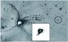 |
Fig. 3 The notable surface brightness features discussed in the text are marked on an extract of the SOFI Ks image. The position of the semi-stellar source is marked in the centre of the bright nebulosity (white in the figure) surrounding it. The YSO_SE filament is shown with a line in the insert. The contours in the insert delineate the central source. The continuous curve marks the ring-segment-like structure facing the NX Pup and the dashed curves the brightest filaments emanating from the YSO. The faint surface brightness patch is inside the circle in the right. |
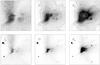 |
Fig. 4 SOFI JHKs images of the CG 1 YSO. The lower panels show the original image. The filter is indicated in the upper left corner of each panel. The size of the lower panels is 46″ by 46″. The upper panels (23″ by 23″) show surface brightness contours overlayed on Gaussian smoothed images. The line in the upper Ks panel shows the orientation of the SOFI slit on the nebulosity (see Sect. 3.2). The cross in all the panels indicates the position of the semistellar YSO. The contour levels in SOFI counts are: Js: 2 to 5 by 1 and (in white) 6; H : 3 to 23 by 5, (in white) 28, 36, 50, 70; Ks: 3 to 23 by 5, (in white) 28 to 112 by 16, and 200 to 600 by 80. |
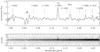 |
Fig. 5 Part of the SOFI spectrum over the YSO and its associated nebulosity in both two dimensional and extracted format. Lower panel: 12″ centre part of the low-resolution long-slit spectrum through the YSO and the YSO SE_filament. Upper panel: extracted continuum-subtracted spectrum convolved with a 3-pixel box-car. The wavelengths of the H2 lines within the displayed spectral region and of the Brγ line are indicated. The spectrum has been normalized for an (1–0) S(1) intensity of unity.The horizontal bar at 2.01 μm indicates the extent of the strong atmospheric absorption between the H and Ks bands. |
3.3. H2 imaging
The difference between the images obtained using the narrow filter NB H2 S1 covering the H2 1–0 S(1), 2.12 μm line and the adjacent continuum obtained with the filter NB 2.090 reveals two objects. The stronger one lies at the centre of the YSO nebulosity and another 90″ west of it. The latter coincides with the faint surface brightness patch, which is seen in the SOFI images in all three colours and noted in Sect. 3.1. An extract of the NB H2 S1 image and the NB H2 S1 – NB 2.090 difference image covering the two objects is shown in the two upper panels in Fig. 6. The cross in the middle panel shows the position of the YSO. The stars and the strong surface brightness surrounding the YSO are cancelled out and only a small size source in the direction of the YSO and a faint patch west of it remain in the difference image. The lowest panel shows the difference image smoothed by a three-pixel half-width Gaussian.
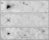 |
Fig. 6 H2 emission in the CG1 head. The upper panel shows an extract of the image obtained with the SOFI NB H2 S1 filter. The centre panel shows the difference NB H2 S1 – NB 2.090. The cross shows the position of the YSO in the Ks image. The lowest panel shows the difference image smoothed with a three-pixel half-width Gaussian. |
3.4. Photometry
The JHKs colour–colour diagram for stars in the CG 1 head is shown in Fig. 7, left panel. The main-sequence (Bessell & Brett 1988) transformed to the 2MASS photometric system is also plotted. The arrow shows the effect of 5m of visual extinction in the diagram according to the Bessell & Brett (1988) reddening law. A small symbol is used if the (J-H) and/or the (H-Ks) formal error is larger than 0.m1. The right panel shows the colour–colour diagram for stars in the reference position.Normal reddened main-sequence stars should lie near or between the reddening lines indicated with dashed lines in Fig. 7. Stars with circumstellar shells and disks have infrared excess and lie to the right of the reddening line. Carbon stars, long period variables, and extragalactic sources may mimic infrared excess sources (Foster et al. 2008). Even though the obvious extragalactic sources were filtered out from the original data set it is highly likely that some of these sources remain in the final data set. The two stars in CG 1 that lie to the right of the reddening line in Fig. 7 are faint (Js ~ 20.m7) and were possibly not recognised as extended sources. If these objects were stars associated with CG 1, they would have to be extremely faint (substellar). An unreddened M5 star at a distance of 300 pc has an apparent J magnitude of 14.6.
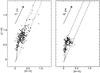 |
Fig. 7 Left: JHKs colour–colour diagram for stars in the CG 1 head. The stars with (J-H) and/or (H-Ks) error larger than 0.m1 are plotted using a small size symbol. The Bessell & Brett (1988) main-sequence transformed to the 2MASS photometric system is also plotted. The arrow shows the effect of 5m of visual extinction in the diagram according to the Bessell & Brett (1988) reddening law. Right: as on the left, but for stars observed at the reference position. |
3.5. C18O mapping
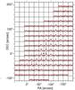 |
Fig. 8 The observed C18O(1–0) (in black) and (2–1) (in red) spectra. The spectra are plotted in the main-beam brightness scale from 1.0 km s-1 to 6.0 km s-1 in velocity and from –0.5 K to 2.8 K in temperature. The positional offsets are in arcseconds from 7h19m283 –44o35′68 (J2000), which is 45 north of NX Pup. The filled circle indicates the position of the YSO in the plot. |
The observed C18O(1–0) (in black) and (2–1) (in red) spectra are shown in Fig. 8. The spectra are plotted in the main-beam brightness scale from 1.0 km s-1 to 6.0 km s-1 in velocity and from –0.5 K to 2.8 K in temperature. The positional offsets are arcseconds from 7h19m283 –44o35′68 (J2000), which is 45 North of NX Pup. The map centre position is the same as in HSHWSP molecular line maps. Contour maps of the C18O(1–0) and (2–1) emission are shown in Figs. B.1 and B.2. The distribution of the C18O(1–0) emission in Figs. 8 and B.1 is consistent with that shown in HSHWSP, Fig. 1. The differences can be attributed to the coarse sampling used by HSHWSP (40″ compared to the 20″ spacing in this paper). In addition the low value of the HSHWSP maximum integrated C18O(1–0) line integral, which is less than 50% of the present data, may be explained in a similar way.
A contour map of the integrated C18O(2–1) emission in the main-beam brightness scale superimposed on the SOFI Ks image is shown in Fig. 9. The contours are from 0.4 K km s-1 to 2.4 K km s-1 in steps of 0.4 K km s-1. The distribution of the emission is elongated with a sharp maximum SW of the YSO. The general C18Odistribution correlates well with the optical extinction evident in the SOFI Js image (Fig. A.1).
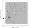 |
Fig. 9 Contour map of the C18O(2–1) integrated emission (main-beam brightness scale) overlaid on the Ks SOFI image. Contour levels are from 0.4 K km s-1 to 2.4 K km s-1 in steps of 0.4 K km s-1. SEST HPBW at the C18O(2–1) frequency is indicated in the upper right. The positional offsets are in arcminutes from NX Pup indicated with a filled circle. |
The C18O (1–0) and (2–1) spectra at three positions are shown in Fig. 10. The offset from the map centre position is shown in arcseconds at the upper left corner of each panel. The velocity marker at the top of each panel is at velocity 3.4 km s-1. The offset positions (–20″, –40″), (–80″, 20″) and (–140″, 80″) are referred to as SE, centre and NW positions, respectively. In Fig. 10, the C18O(2–1) line intensity is significantly stronger than the C18O(1–0) intensity at the SE and centre positions. However, the centre of line velocities are different, 3.69 ± 0.03 km s-1 at SE and 3.33 ± 0.03 km s-1 at the centre position. Also the line widths differ being 0.46 km s-1 and 0.70 km s-1 at the two positions, respectively. The velocity difference was seen by HSHWSP in 12CO and here it is confirmed in the C18O emission. At the NW position, the intensities in the two transitions are equal and the line velocity is similar to that at the centre position. The lines are asymmetric (blue wing at centre position, and red at NW position).
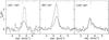 |
Fig. 10 C18O(2–1) (histogram) and (1–0) (line) spectra in three positions. The offset from the map centre is indicated in the upper left corner of each plot. The velocity marker at the top of each panel is at velocity 3.4 km s-1. |
4. Discussion
4.1. C18O mapping
In the following discussion, the C18Omap is divided into three regions: 1) C18O_SE (the 3.7 km s-1 velocity component is dominant); 2) C18O_maximum (the integrated C18Oemission maximum); and 3) C18O_NW (region in the NW where the C18O (1–0) and (2–1) TMB intensities are similar).
In the LTE approximation, the C18Oline intensity depends on both the C18Ocolumn density and the C18Oexcitation temperature, whereas the C18O(1–0) to C18O(2–1) intensity ratio depends on the excitation temperature. If the C18Oexcitation temperature were constant in the mapped area, the integrated line area of the optically thin C18Oemission would trace the cloud gas column-density linearly. However, the C18Opeak TMB(2–1)/TMB(1–0) ratio varies over the map. In Figs. 8 and 10, the C18O (2–1)emission is significantly stronger than the C18O(1–0) emission in the direction of the C18O_maximum and in C18O_SE. In C18O_NW, the intensity of the two transitions is the same. The varying line ratio indicates that the excitation temperature is higher in both C18O_maximum and C18O_SE than in C18O_NW.
The interaction of the newly born star with the surrounding cloud (see the discussion below) would be a likely reason for a warmer spot in the cloud (C18O_maximum). The C18Oline width is also the broadest in C18O_maximum, which is indicative of extra turbulence at this position. The C18O line velocity in C18O_SE differs from that in C18O_maximum, implying that these are separate structures in the cloud. The high NIR surface brightness around C18O_SE in Figs. 1 and 2 indicates that the radiation from the star NX Pup is the reason for the elevated temperature. C18O_NW lies NW of the YSO and the C18O_maximum and is most probably well shielded against the radiation from NX Pup. This region of the cloud would correspond to a quiescent, low temperature part of the cloud.
The C18O(2–1) emission is distributed in a north-south oriented ridge, which is inconsistent with a point-like source. It can be seen in Figs. 8 and 9 that the C18O(2–1) maximum does not fall on the measuring grid but lies slightly NE of the measured maximum line integral and west of the location of the YSO. If the C18Omaximum were point-like, it would be justifiable to argue that the positional offset between the maximum and the YSO would be caused by a larger than expected telescope pointing error during the observations. However, the maximum is elongated and there is no obvious reason why the north-south oriented C18Oridge should be centred on the YSO position. The C18Omapping grid spacing is only marginally finer than the SEST beam HPBW at the C18O(2–1) frequency (grid 20″, HPBW 23″) and therefore a fully sampled map is needed to pinpoint the exact location of the maximum.
The HCO + (4–3) line observed by van Kempen et al. (2009) in the direction of the YSO is weak (TMB 0.6 K) and H13CO + (4–3) was a upper limit of 0.08 K. This rules out a dense core in this direction (van Kempen et al. 2009). Even though the position where van Kempen et al. (2009) observed the C18O(3–2) and the HCO + (4–3) lines, the YSO, lies between the mapping positions in this paper, their measurement can be used to evaluate the nature of the C18O_maximum. The APEX beam size at 319 GHz is similar to the SEST beam size at 220 GHz, which makes comparing the line intensities observed with APEX and SEST realistic. The APEX C18O(3–2) TMB line intensity, 2.3 K, is similar to the SEST C18O(2–1) line intensities observed around the YSO. Because the C18O(3–2) line temperature is low, the C18O_maximum position cannot be a C18Ohotspot similar to that discovered in CG 12 (NGC 5367) (Haikala et al. 2006). Even though the emission from high density tracers is weak in the CG 12 C18Ohotspot, the C18O (3–2) TMB of 10 K is high compared to the TMB temperatures in the (2–1) and (1–0) transitions (5 K and 2.2 K, respectively). Observations of the high density tracers (van Kempen et al. 2009) and C18Othus indicate that C18O_maximum is a moderately dense elongated structure west of the YSO position.
4.2. Visual extinction
The NICER method presented in Lombardi & Alves (2001) and the SOFI NIR photometry can be used to estimate the visual extinction within the imaged area in CG 1. However, the position of CG 1 14o below the Galactic plane is unfavourable for applying the NICER method because the expected number of bright background stars, especially of giant stars, is low. Therefore the spatial resolution of the resulting extinction map is only 20″. The J – H/H – Ks colour–colour diagram for the observed off-field is shown in Fig. 7, right panel. The diagram shows that the interstellar extinction is small in the off-field direction. The field lies at the same Galactic latitude as the on-field and therefore the stellar population should be statistically similar to that of the on-field. Thus the off-field is well suited to being used in the NICER method. The contour map (thick lines) of the extinction derived for the CG 1 head superimposed on the SOFI Ks image is shown in Fig. 11. The contours are from 2.m0 to 9.m0 in steps of 1.m0. The contours of the C18O(2–1) integrated emission (0.8 K km s-1 to 2.4 K km s-1 in steps of 0.4 K km s-1) are shown with thin lines. The minimum visual extinction, 1.m3, in the map is in the NE corner of the image. This non-zero minimum extinction agrees with Fig. 7, where practically all late main sequence stars are above the main-sequence also plotted in the figure. The maximum extinction, 9.m2, is located NW from the YSO. However, a word of caution is required because the NICER method assumes that the extinction is constant in each NICER cell (in this case 20″ by 20″). If a cell contains a compact (with respect to the cell size) high extinction structure, the measured extinction tends to be biased towards lower extinction (Lombardi 2005). Thus, localised small-size extinction maxima may go unnoticed.
The position of the maximum extinction does not coincide with the maximum C18Ointegrated emission (Fig. 9). This shows, as discussed in Sect. 4.1, that because of the varying C18Oexcitation temperature the distribution of the observed C18Ointegrated emission does not linearly trace the gas/dust column density distribution. In addition, the optical extinction also traces the low density cloud envelope where C18Omolecule is not excited.
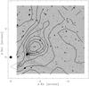 |
Fig. 11 Contour map of the optical extinction (thick lines) obtained with the NICER method overlaid on the Ks SOFI image. Contour levels are from 2 mag to 9 mag in steps of 1 mag.Contours of the C18O(2–1) integrated emission (0.8 K km s-1 to 2.4 K km s-1 in steps of 0.4 K km s-1) are shown with thin lines. The positional offsets are as in Fig. 9. |
4.3. Column densities and masses
A detailed three-dimensional non-LTE model that accounts for both the varying density and excitation conditions would be necessary to derive the cloud physical properties. The construction of this model is not possible because only C18O (1–0) and (2–1) mapping data can be used and only a few pointed observations are available for other molecules. The LTE-approximation approach is used instead of a sophisticated model to obtain a zeroth-order estimate of the H2 column densities and masses. An average C18Oexcitation temperature for C18O_SE, C18O_maximum, and C18O_NW is estimated assuming optically thin C18Oemission and using the observed relative C18O(2–1) and (1–0) line intensities. This assumes that the observed emission in both transitions originates in the same volume of gas at a constant excitation temperature. The observed C18Oline TMB(2–1)/ TMB(1–0) ratio is 2 in C18O_SE and C18O_maximum, which is compatible with an excitation temperature near 15 K. In C18O_NW, the ratio is one indicating an excitation temperature of the order of 10 K. The low C18O(2–1) TMB temperature in C18O_NW may also be due to subthermal excitation. However, according to model calculations presented in Warin et al. (1996), the deviation of the populations in the lowest C18Oenergy levels from their LTE values is small in typical conditions prevailing in dark clouds. Considering the high H2 column density derived for C18O_NW from optical extinction (see below), subthermal excitation is unlikely.
The N(H2) column density can be estimated using both the C18Odata and the optical extinction. The relation between the molecular hydrogen and C18Ocolumn density is N(H2) = [ N(C18O)/1.7 × 1014 + 1.3 ] 1021 (Frerking et al. 1982). Assuming LTE and C18Oexcitation temperature of 15 K in C18O_SE and C18O_maximum and 10 K in C18O_NW, the peak N(H2) column densities in these regions are 5.0 × 01021 cm-2, 7.8 × 1021 cm-2, and 4.9 × 1021 cm-2, respectively. The relation between the optical extinction and hydrogen column density is N(H) = 2 × 1021 cm-2 mag-1 (Bohlin et al. 1978). The peak N(H2) column density estimated from the extinction data is 9.0 × 1021 cm-2. The maximum is in the direction of C18O_NW and is nearly twice that estimated from the C18Odata.
The LTE column densities can be compared with those calculated with a non-LTE radiative transfer code such as RADEX (van der Tak et al. 2007), which is available on-line. The C18O(1–0) and (2–1) line intensities are calculated by providing the kinetic temperature, H2 number density, the C18Ocolumn density, and the C18O line width as input parameters. The line width is known in CG 1 and a H2 number density of 104 cm-3 is a reasonable guess. The observed C18O(2–1) to C18O(1–0) line intensities in C18O_NW can be reproduced with RADEX assuming a C18O10 K excitation temperature and the LTE column density calculated above. However, in C18O_SE and C18O_maximum the C18Oexcitation temperature has to be increased from 15 K to 30 K to make the line intensities agree. This is because of subthermal excitation of the C18O(2–1) transition. Increasing the N(H2) column density makes the C18O(1–0) line stronger in respect to the C18O(2–1) line which does not agree with the observations. The comparison of LTE and non-LTE results shows that the two methods produce similar N(H2) column densities if the input kinetic temperature is adjusted. The conversion factor from the line integral to column density in the LTE method is temperature dependent but the variation is only 20% in the 10 K to 30 K range.
The cloud mass can be calculated from the C18Odata by summing up the calculated N(H2) column densities point by point and using the mean molecular weight per H2 molecule 2.8. A major uncertainty in the mass calculation is the distance to CG 1, as the mass scales as the square of the distance. If the distance d to CG 1 is 450 pc instead of the assumed 300 pc, the calculated mass more than doubles. Assuming C18Oexcitation temperatures as above, the masses of C18O_SE, C18O_maximum, and C18O_NW are 0.75 M⊙ (d/300 pc)2, 1.35 M⊙ (d/300 pc)2, and 1.6 M⊙ (d/300 pc)2, respectively. These numbers should be considered very rough estimates because the regions overlap and the division of data between them is subjective. The masses are lower limits because they refer to gas traced by the C18Oemission. The true masses are higher as the clumps have low density envelopes that are not detected in C18O. The most massive of the three regions is C18O_NW. The C18Oline intensity in its direction is lower than in the other two regions but this is compensated by its larger size.
Summing up the extinctions point by point, using the Bohlin et al. (1978) relation between the extinction and hydrogen column density and mean molecular weight per H2 molecule 2.8, the total mass from the extinction data in the imaged area is 16.7 M⊙ (d/300 pc)2. The Av = 4 mag contour covers approximately the area observed in C18O. The mass within this contour is 9.2 M⊙ (d/300 pc)2, which is more than twice the summed up C18Omass. The discrepancy between the masses calculated from the extinction data and the C18Odata is expected because the optical extinction also traces the low density cloud envelope, which is not detected in C18O.
4.4. Spectroscopy and narrow-band imaging
The SOFI spectrum was taken to investigate the nature of the nebulosity, i.e., ascertain whether it is only reflected light or whether line emission is also present. The spectrum in Fig. 5 shows an underlying continuum, at least three H2 lines, and the Brγ line. The H2 line emission does not only originate in the location of the YSO but also from the base of the YSO_SE filament. The spectral resolution and the spectrum low signal-to-noise ratio do not allow us to extract detailed physical information, though by comparing with the models of e.g. Smith (1995) we note that the line strengths of the H2 lines appear more consistent with C-type shocks than J-type. As expected, the Brγ line emission is seen only in the direction of the YSO as this line is expected to originate very near the YSO (see e.g. Malbet 2007). The underlying continuum emission is direct light from the YSO and light reflected from the surroundings. The spectrum is not sensitive enough to show the continuum in the direction of the SE filament.
The H2 emission region can also be seen in the narrow-band H2/continuum difference image in Fig. 6. It is centered on the Ks YSO and is resolved in the E-W direction but not in the N-S direction. The extent in the E-W direction is 5″. The NIR spectrum shows that H2 emission comes also from the base of the YSO_SE filament but the narrow-band images are not deep enough and emission in Fig. 6 is confined only to the YSO.
For the offset 90″ west from the YSO, a faint patch of emission is detected. This patch coincides with those seen in the Js and H bands (Sect. 3.1). The difference image in Fig. 6 shows that in the Ks band this emission is mostly due to H2 line emission. Though this object is likely to be a HH-object it cannot be confirmed in the optical. Therefore it will be designated as a molecular hydrogen emission-line object MHO 1411, (Davis et al. 2010).
4.5. IRAS 07178–4429
CG 1 was mapped by the IRAS satellite in wavelengths 12 to 100 μm. Besides extended surface emission, IRAS detected a point source, IRAS 07178–4429, at the edge of the globule head. The non-colour-corrected fluxes of the point source are 6.68, 7.60, 13.12, and 33.59 Jy at 12, 25, 60, and 100 μm, respectively. The positional uncertainty ellipse major and minor axis are 10″, 3″ and the position angle (East through North) 178°. The 60 and 100 μm fluxes point to an embedded source. However, considering the 100 μm flux of 33.59 Jy, the 12 μm flux of 6.68 Jy is too strong for such a source.
The spatial resolution of original IRAS images can be enhanced using HIRES processing, which uses the maximum correlation technique (Auman et al. 1990). Figure 12 displays contour maps of the CG1 HIRES processed (20 iterations) IRAS maps superimposed on the SOFI Ks band image. The IRAS wavelength in microns is shown in the upper left corner of each panel and the position of the star NX Pup is marked with a filled circle. The IRAS 07178–4429 point-source positional uncertainty ellipse is shown in the 100 μm panel. It lies west of NX Pup at the edge of the Ks image. The C18O(2–1) integrated emission contours (1.2 K km s-1 to 2.0 K km s-1 in steps of 0.4 K km s-1) are superimposed on the 12 μm panel. The 12 μm IRAS contours in Fig. 12 are centred on the star NX Pup. At 25 μm, the maximum contours are still centred on NX Pup but at a lower level the contours encircle the YSO. At 60 and 100 μm, the maximum of the emission has shifted significantly to the west of NX Pup and lies near the YSO and the maximum of the C18O(2–1) integrated emission. The nominal point source position lies between the 12–25 μm and the 60–100 μm maxima.
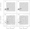 |
Fig. 12 Contour maps of the HIRES processed IRAS maps superimposed on the SOFI Ks band image. The IRAS wavelength is shown in microns in the upper right corner of each panel. The position of the star NX Pup is marked with a filled circle. The IRAS 07178–4429 point source positional uncertainty is shown as an filled ellipse west of NX Pup in the 100 μm panel. The C18O(2–1) integrated emission contours (indicated by thick lines, 1.2 K km s-1 to 2.0 K km s-1 in steps of 0.4 K km s-1) are superimposed on the 12 μm panel. The offset is in arcminutes from the centre of the SOFI image. The contour levels in MJy sr-1 are: 12 μm 5 to 30 by 5; 25 μm 15 to 115 by 20; 60 μm 3, 5, 15 to 91 by 19; and 100 μm 7, 16, 31 to 71 by 20. |
The likely explanation of the disagreement between the point source fluxes (hot or cold source) and the systematic shift of the position of the IRAS emission maximum from 12 μm to 100 μm is that there are two sources, one warm (NX Pup) and one cold (the YSO). Spitzer 24 and 70 μm MIPS observations now available online confirm the HIRES analysis. Spitzer detected two sources, one centered on NX Pup and another at the YSO. Their relative flux ratios (YSO/NX Pup) are ~0.64 (24 μm) and ~100 (70 μm). A similar case of two infrared sources observed as one IRAS point source is observed in CG 12 (NGC 5367). The Herbig AeBe binary star h4636 and an adjacent cold source are merged into a single source, IRAS 13547-3944 (Haikala & Reipurth 2010).
The IRAS 12, 25, 60, and 100 μm point source catalog fluxes in janskys can be converted into in band fluxes by multiplying them with the synthesized IRAS bandpasses of 2.06 × 10¹³ Hz, 7.56 × 10¹² Hz, 4.55 × 10¹² Hz, and 1.74 × 10¹² Hz, respectively (Emerson 1988) and the source luminosity can be calculated.Though the Spitzer 70 μm and the IRAS 60 μm bandpasses are not the same, it can be assumed that the contribution of NX Pup to the IRAS 60 μm flux is not significant. Using the IRAS 07178–4429 60 and 100 μm fluxes the FIR luminosity of the YSO is 3.1 L⊙ × (d/300 pc)2.
There are two secondary maxima in addition to the IRAS point source at 60 μm in Fig. 12. These lie at the globule bright edge seen in Fig. 2. In the three-component dust model (Puget & Leger 1989), interstellar dust consists of large aromatic molecules (PAHs), very small grains (VSGs), and the classical large grains. The VSGs are transiently heated and emit non-thermal emission in the mid- to FIR. In dark clouds (temperatures < 20 K), the large grains emit in thermal equilibrium at wavelengths ≥ 80 μm. The two secondary 60 μm maxima in Fig. 12 are therefore most likely to be produced by VSGs at the surface of the globule and heated by the star NX Pup or the UV radiation from the central part of the Gum nebula. Consistent with the HIRES 60 μm image the globule bright edges can also be seen in the Spitzer 70 μm image. In addition, the bright reflection nebulosity at the SE tip of CG 1 seen in Fig. 1 appears as a bright, extended source in the Spitzer 70 μm image. This extended emission is likely to be due to VSGs heated by NX Pup. This would also agree with the argument presented in Sect. 4.1 that the radiation from NX Pup explains the elevated C18Oexcitation temperature in C18O_SE. The Spitzer 70 μm integrated flux from C18O_SE is similar to that of NX Pup and does not invalidate the YSO IRAS FIR luminosity calculation presented above.
4.6. NX Pup–cloud interaction
The HAEBE star NX Pup lies north of the bright “nose” nebulosity and east of the obscured CG 1 globule head. Being close to CG 1, the star NX Pup dominates the local radiation field over the general interstellar radiation field at least around the globule head. Two surface brightness features in CG 1 indicate that the position of the star near the globule is not a projection effect but that the star is physically located near the globule. It is likely that the illuminating source of the very bright reflection nebulosity at the SE tip of CG 1 seen in Fig. 1 and the corresponding Spitzer 70 μm surface brightness is NX Pup. The star may also be the reason for the elevated C18Oexcitation temperature of C18O_SE. The second surface brightness feature is the arc reaching NE from the YSO. The arc is symmetric with respect to NX Pup and is also seen in the optical images, not only in NIR. The arc could indicate the edge of a bubble vacated from gas and dust by NX Pup.
4.7. YSO properties
In the SOFI imaging, the YSO is visible only at Ks. In H and Js, it lies behind an obscuring dust lane (Figs. 4 and A.4). Therefore its (J – H) and (H – K) colour indices cannot be calculated and its position in the JHKs colour–colour diagram is not known. The YSO 2Mass Ks magnitude is 13.m42, which is consistent with the SOFI photometry. The SOFI imaging H limiting magnitude is 20.m5 but because the YSO lies at the centre of a very bright nebulosity the limiting magnitude is brighter at its position. A conservative estimate of the minimum (H – K) colour index would be ≳6 mag. The average intrinsic (H – K) colour index for the SOFI off-field in Fig. 7 is 0.m15. The YSO visual extinction calculated with the NICE method (Lada et al. 1994) would be ~93 mag. This is however an upper limit as the object most probably has an infrared excess (the extent of the YSO source profile in the EW direction is nearly twice that of isolated stars elsewhere in the image (Sect. 3.1). Despite the IR excess, the visual extinction towards the YSO is likely to be more than 50 mag. This extinction is significantly higher than the maximum extinction in the CG 1 head (9.m2) and the estimated extinction in the direction of the YSO (~6 mag) as estimated with the NICER method in Sect. 4.2. If the extinction takes place in a compact circumstellar disk or a circumstellar shell it would not be detected with the NICER method.
The van Kempen et al. (2009) pointed molecular line observations of the IRAS 07178–4429 point source were aimed at detecting the possible associated protostellar envelope/core and molecular outflow. The position observed by van Kempen et al. (2009) was however the YSO and not the nominal IRAS point source position. This pointing was possibly selected using the CG 1 Ks image in Santos et al. (1998). van Kempen et al. (2009) found evidence of neither protostellar envelope nor a molecular outflow and concluded that it is most likely not an embedded YSO (class I source). This indicates that the observed high extinction towards the YSO takes place in a circumstellar disk and not in a circumstellar shell. This makes the source a likely class II source.
4.8. YSO–cloud interaction: where is the outflow?
Besides mass infall, the early stage of low-mass star formation is also associated with energetic mass outflows. Manifestations of outflows are observed, e.g., as jets, molecular outflows and Herbig-Haro objects. The outflows inject momentum and energy into the parent cloud and can have a highly disruptive effect on the cloud core they are forming in.
Molecular hydrogen emission detected in the low-mass star-formation regions is usually associated with shocks due to hot and dense gas flowing out from the newly born stars. The H2 NIR line emission can also be due to UV absorption and fluorescence (Black & Dalgarno 1976). Fluorescent H2 line emission has been observed in elephant trunks in HII regions (e.g. Allen et al. 1999). The fluorescent H2 emission appears as a bright, thin layer on the surface of the trunks on the side facing the ionizing source. However, the ionizing source is missing in CG 1. The FUV spectrum of NX Pup is most consistent with a spectral type F2III (Blondel & Djie 2006). Thus the UV flux from NX Pup cannot ionize the cloud surface. It is also not plausible that the early-type stars ionizing the Gum nebula would excite only a very localized region in CG 1. This leaves shock excited H2 as the only viable option. On similar grounds, MHO 1411, which lies 90″ west of the YSO, is likely to be a highly obscured Herbig-Haro object. The higher C18Oexcitation temperature around the YSO relative to C18O_NW also points to an additional energy source, probably the YSO. An indirect indication of shocks is the [HCN]/[HNC] molecular abundance ratio being found to be larger than 1 by HSHWSP. Such a ratio can be produced by shock chemistry.
Even though the typical tracers of an outflow are present (molecular hydrogen and Brγ line emission indicating shocks and a probable heavily obscured HH object), actual outflow can be seen neither in the HSHWSP CO velocity interval plots nor the van Kempen et al. (2009) CO (3–2) spectrum in the direction of the YSO. The ESO data archive contains a ~1′ by 15 on the fly and a smaller pointed CO (3–2) mapping in the direction of the YSO observed at APEX (ESO project 077.C-0217A, van Kempen et al.). A regridded, summed-up CO (3–2) map is shown in Fig. C.1. No obvious molecular outflow can be seen in this data set. The CO (3–2) (histogram) spectrum in the direction of the YSO is shown in Fig. 13. There is an indication of a very modest redshifted outflow wing in the spectrum. However, part of this wing may be caused by a second cloud velocity component seen in the lower left in Fig. C.1. The second spectrum (line plot) in the figure is a sum of the CO (3–2) spectra in a ± 10″ EW slice in declination through the YSO. The 0, 0 position is not included in the sum. A Hanning-smoothed C18O(3–2) 0, 0 position spectrum from the same data set is also shown in the figure. The morphology of the YSO nebulosity in the SOFI images and especially the location of MHO 1411 west of the YSO implies that the associated molecular outflow, if present, should be oriented in the EW direction. However, there is no indication of outflow wings in the declination-slice summed-up spectrum. In contrast, it is more narrow than the spectrum in the centre position. The C18O(3–2) spectrum is centred on the CO line.
It is puzzling why no molecular outflow from the YSO is detected. If an outflow were present, it would have to be highly collimated and exactly in the plane of the sky to remain unnoticed.
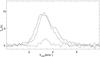 |
Fig. 13 APEX CO (3–2) spectra in the direction of the YSO (histogram) and in a ± 10″ slice in declination (0, 0 position excluded) (line) and a Hanning smoothed C18O(3–2) spectrum of the centre position. The temperature unit is |

5. Summary and conclusions
We have combined our new NIR imaging, photometry, spectroscopy, and mm molecular line observations with already existing data at other wavelengths to analyse the structure of the globule head in greater detail than possible before. The conclusions are the following:
-
1.
A young stellar object (a likely class II source)with an associated bright NIR nebulosity and a molecularhydrogen object, MHO1411, were detected in the globule head.The YSO is totally obscured in Js. The estimated optical extinctiontowards the YSO is 50 magnitudes or more. TheH2 and Brγ line emission is detected in the direction of the YSO. The H2 emission is also seen in the YSO_SE filament;
-
2.
The visual extinction, as estimated with the NICER method, in the imaged area excluding the YSO direction, ranges from 1.m3 to 9.m2 magnitudes. The maximum extinction lies 40″ NW of the YSO. The peak N(H2) column density estimated from the extinction data is 9.0 × 1021 cm-2 and the total mass 16.7 M⊙(d/300 pc)2. The mass within the Av = 4 mag contour is 9.2 M⊙(d/300 pc)2;
-
3.
The C18Oemission in the globule head is distributed in an 15 by 4′ area with a sharp maximum offset SW of theYSO. The C18OTMB(2–1) is equal to TMB(1–0) in the NW part of the cloud (the Av maximum) but is significantly stronger than in the C18O(1–0) transition in the C18Omaximum and in the SE. This indicates that the C18Oexcitation temperature is higher in the latter two positions. The C18Ocentre of line velocity is 3.33 ± 0.03 km s-1 in the C18Omaximum and 3.69 ± 0.03 km s-1 in SE indicating, that these are physically separate entities. It is likely that the elevated C18Oexcitation temperature SW of the YSO is caused by the interaction of the YSO with the surrounding cloud. The SE “nose” coincides with a bright reflection nebulosity south of NX Pup in the SOFI and SIRIUS images. An elevated C18Oexcitation temperature in the “nose” is likely because of heating by NX Pup;
-
4.
The peak N(H2) column densities and masses, as calculated from the C18Odata, are (5.0 × 1021 cm-2, 0.75 M⊙ (d/300 pc)2), (7.8 × 1021 cm-2, 9.2 M⊙(d/300 pc)2) and (1.35 × 1021 cm-2, 1.6 M⊙(d/300 pc)2) for C18O_SE, C18O_maximum, and C18O_NW, respectively. The column densities and the masses are calculated from only two C18Otransitions and should be considered as very rough estimates. The C18Omasses are lower than those calculated from the extinction data. The likely reason for this is that the cloud low density envelope is not visible in C18O;
-
5.
The peak integrated C18Oemission does not coincide with the position of maximum visual extinction. This is primarily due to the C18Oexcitation temperature, which is lower in the extinction maximum than in the C18Oemission maximum;
-
6.
The IRAS point source 07178–4429 resolves into two sources in the HIRES enhanced IRAS images. The 12 and 25 μm emission originates mainly in the Herbig AeBe star NX Puppis and the 60 and 100 μm emission in the adjacent YSO.The results of the HIRES analysis are confirmed by Spitzer 24 μm and 70 μm MIPS mapping, which has become publicly available. The 60 and 100 μm FIR luminosity of the point source is 3.1 L⊙;
-
7.
Even though typical signs of YSO–parent cloud interaction (shocked gas, elevated C18Oexcitation temperature, MHO object) were detected no strong molecular outflow seems to be present;
-
8.
If the binary NX Pup and the T Tau star adjacent to it were formed in CG 1, they have already cleared away the surrounding dust and molecular gas. The YSO detected in NIR in the globule head is the second generation of stars formed in the cloud.
The new NIR photometry and molecular line data presented in this paper reveal a newly born star and a rather complex distribution of interstellar material in the globule head. However, the derived cloud parameters, e.g., mass, column density, and excitation temperature, are only rough estimates. Further observations are necessary to refine the cloud model. Mapping of the cloud head in density sensitive molecules and in both FIR and (sub)mm continuum is needed to have sufficient input parameters to run a radiative transfer code like e.g. the one presented in Juvela (1997). Additional NIR imaging and spectroscopy are needed to provide information on the nature of the YSO and the surrounding nebulosities.
Online material
Appendix A: Sofi imaging
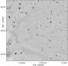 |
Fig. A.1 SOFI Js image of CG 1 head. Square root scaling has been used to enhance the appearance of the faint surface brightness structures. |
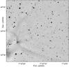 |
Fig. A.2 SOFI H image of CG 1 head. Square root scaling has been used to enhance the appearance of the faint surface brightness structures. |
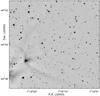 |
Fig. A.3 SOFI Ks image of CG 1 head. Square root scaling has been used to enhance the appearance of the faint surface brightness structures. |
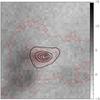 |
Fig. A.4 SOFI Ks (in black) and H (in red) surface brightness contours superimposed on a grey scale Js image. The contour levels in SOFI counts are from 100 to 1100 in steps of 100 in Ks and from 10 to 90 in steps of 10 in H . The wedge in the right shows the Js grey scale levels. The image size is 23″ by 23″ and SOFI pixel scale is 0288. |
Appendix B: C18O mapping
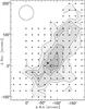 |
Fig. B.1 Contour map of the integrated C18O(1–0) emission in CG 1 head in TMB scale. The contour levels are from 0.25 K km s-1 to 1.25 K km s-1 in steps of 0.25 K km s-1. The points indicate the measured points and the square the location of the YSO in the figure. The SEST HPBW at the C18O(1–0) frequency is shown in the upper left corner. |
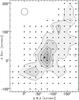 |
Fig. B.2 Contour map of the integrated C18O(2–1) emission in CG 1 head in TMB scale. The contour levels are from 0.4 K km s-1 to 2.0 K km s-1 in steps of 0.4 K km s-1. The points indicate the measured points and the square the location of the YSO in the figure. The SEST HPBW at the C18O(2–1) frequency is shown in the upper left corner. |
Appendix C: ESO archive data
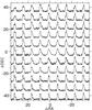 |
Fig. C.1 CO (3–2) map in the direction of the YSO. The spectra are plotted from 1 km s-1 to 7 km s-1 in velocity and from –1 K to 12 K in |
Acknowledgments
It is a pleasure to thank the NTT team for the support during the observing run. This research has made use of the SIMBAD database, operated at CDS, Strasbourg, France, and of NASA’s Astrophysics Data System Bibliographic Services.This work is based in part on archival data obtained with the Spitzer Space Telescope, which is operated by the Jet Propulsion Laboratory, California Institute of Technology under a contract with NASA. M.M acknowledges the support from the University of Helsinki Senat’s graduate studies grant and from the Vilho, Yrjö and Kalle Väisälä Fund.
References
- Allen, L. E., Burton, M. G., Ryder, S. D., Ashley, M. C. B., & Storey, J. W. V. 1999, MNRAS, 304, 98 [NASA ADS] [CrossRef] [Google Scholar]
- Ascenso, J., Alves, J., Vicente, S., & Lago, M. 2007, A&A, 199 [Google Scholar]
- Auman, H., Fowler, J., & Melnyk, M. 1990, AJ, 99, 1674 [NASA ADS] [CrossRef] [Google Scholar]
- Bernacca, P. L., Lattanizi, M. G., Bucciarelli, B., et al. 1993, A&A, 278, L47 [NASA ADS] [Google Scholar]
- Bertin, E., & Arnouts, S. 1996, A&AS, 117, 393 [NASA ADS] [CrossRef] [EDP Sciences] [Google Scholar]
- Bessell, M., & Brett, J. 1988, PASP, 100, 1134 [NASA ADS] [CrossRef] [Google Scholar]
- Black, J. H., & Dalgarno, A. 1976, ApJ, 203, 132 [NASA ADS] [CrossRef] [Google Scholar]
- Blondel, P. F. C., & Djie, H. R. E. T. A. 2006, A&A, 456, 1045 [NASA ADS] [CrossRef] [EDP Sciences] [Google Scholar]
- Bohlin, R. C., Savage, B. D., & Drake, J. F. 1978, ApJ, 224, 132 [NASA ADS] [CrossRef] [Google Scholar]
- Bourke, T., Hyland, A., Robinson, G., James, S., & Wright, C. 1995, MNRAS, 276, 1067 [NASA ADS] [Google Scholar]
- Brand, P. W. J. L., Hawarden, T. G., Longmore, A. J., Williams, P. M., & Caldwell, J. A. R. 1983, MNRAS, 203, 215 [NASA ADS] [Google Scholar]
- Brandner, W., Bouvier, J., Grebel, E. K., et al. 1995, A&A, 298, 818 [NASA ADS] [Google Scholar]
- Davis, C. J., Gell, R., Khanzadyan, T., Smith, M. D., & Jenness, T. 2010, A&A, 511, A24 [NASA ADS] [CrossRef] [EDP Sciences] [Google Scholar]
- Emerson, J. P. 1988, in Formation and Evolution of Low Mass Stars, ed. A. K. Dupree, & M. T. V. T. Lago, NATO ASIC Proc., 241, 21 [Google Scholar]
- Foster, J. B., Román-Zúñiga, C. G., Goodman, A. A., Lada, E. A., & Alves, J. 2008, ApJ, 674, 831 [NASA ADS] [CrossRef] [Google Scholar]
- Franco, G. A. P. 1990, A&A, 227, 499 [NASA ADS] [Google Scholar]
- Frerking, M. A., Langer, W. D., & Wilson, R. W. 1982, ApJ, 262, 590 [NASA ADS] [CrossRef] [Google Scholar]
- Haikala, L. K., Juvela, M., Harju, J., et al. 2006, A&A, 454, L71 [NASA ADS] [CrossRef] [EDP Sciences] [Google Scholar]
- Haikala, L. K., & Reipurth, B. 2010, A&A, 510, A1 [NASA ADS] [CrossRef] [EDP Sciences] [Google Scholar]
- Harju, J., Sahu, M., Henkel, C., et al. 1990, A&A, 233, 197 [NASA ADS] [Google Scholar]
- Hawarden, T., & Brand, P. 1976, MNRAS, 175, 19P [NASA ADS] [CrossRef] [Google Scholar]
- Juvela, M. 1997, A&A, 322, 943 [NASA ADS] [Google Scholar]
- Lada, C., Lada, E., Clemens, D., & Bally, J. 1994, ApJ, 429, 694 [NASA ADS] [CrossRef] [Google Scholar]
- Lombardi, M. 2005, A&A, 438, 169 [NASA ADS] [CrossRef] [EDP Sciences] [Google Scholar]
- Lombardi, M., & Alves, J. 2001, A&A, 377, 1023 [NASA ADS] [CrossRef] [EDP Sciences] [Google Scholar]
- Nagayama, T., Nagashima, C., Nakajima, Y., et al. 2003, ed. M. Iye, & A. F. M. Moorwood, SPIE Conf. Ser., 4841, 459 [Google Scholar]
- Persson, S. E., Murphy, D. C., Krzeminski, W., Roth, M., & Rieke, M. J. 1998, AJ, 116, 2475 [NASA ADS] [CrossRef] [Google Scholar]
- Puget, J. L., & Leger, A. 1989, ARA&A, 27, 161 [NASA ADS] [CrossRef] [Google Scholar]
- Reipurth, B. 1983, A&A, 117, 183 [NASA ADS] [Google Scholar]
- Sanduleak, N. 1974, Information Bulletin on Variable Stars, 880, 1 [NASA ADS] [Google Scholar]
- Santos, N., Yun, J., Santos, S., & Marreiros, R. 1998, A&A, 116, 1376 [Google Scholar]
- Smith, M. D. 1995, A&A, 296, 789 [NASA ADS] [Google Scholar]
- van der Tak, F. F. S., Black, J. H., Schöier, F. L., Jansen, D. J., & van Dishoeck, E. F. 2007, A&A, 468, 627 [NASA ADS] [CrossRef] [EDP Sciences] [Google Scholar]
- van Kempen, T. A., van Dishoeck, E. F., Hogerheijde, M. R., & Güsten, R. 2009, A&A, 508, 259 [Google Scholar]
- Warin, S., Benayoun, J. J., & Viala, Y. P. 1996, A&A, 308, 535 [NASA ADS] [Google Scholar]
- Zinnecker, H., Krabbe, A., McCaughrean, M. J., et al. 1999, A&A, 352, L73 [NASA ADS] [Google Scholar]
All Figures
|
Fig. 1 Colour–coded SIRIUS image of the CG 1 head. The J, H, and Ks bands are coded in blue, green, and red, respectively. Square root scaling has been used to enhance the faint surface brightness structures. NX Pup is the brightest star in the image at 7h19m283, − 44o35′103. |
| In the text | |
|
Fig. 2 Colour–coded SOFI image of CG 1 head. The Js, H, and Ks bands are coded in blue, green, and red, respectively. Square root scaling has been used to enhance the faint surface brightness structures. |
| In the text | |
|
Fig. 3 The notable surface brightness features discussed in the text are marked on an extract of the SOFI Ks image. The position of the semi-stellar source is marked in the centre of the bright nebulosity (white in the figure) surrounding it. The YSO_SE filament is shown with a line in the insert. The contours in the insert delineate the central source. The continuous curve marks the ring-segment-like structure facing the NX Pup and the dashed curves the brightest filaments emanating from the YSO. The faint surface brightness patch is inside the circle in the right. |
| In the text | |
|
Fig. 4 SOFI JHKs images of the CG 1 YSO. The lower panels show the original image. The filter is indicated in the upper left corner of each panel. The size of the lower panels is 46″ by 46″. The upper panels (23″ by 23″) show surface brightness contours overlayed on Gaussian smoothed images. The line in the upper Ks panel shows the orientation of the SOFI slit on the nebulosity (see Sect. 3.2). The cross in all the panels indicates the position of the semistellar YSO. The contour levels in SOFI counts are: Js: 2 to 5 by 1 and (in white) 6; H : 3 to 23 by 5, (in white) 28, 36, 50, 70; Ks: 3 to 23 by 5, (in white) 28 to 112 by 16, and 200 to 600 by 80. |
| In the text | |
|
Fig. 5 Part of the SOFI spectrum over the YSO and its associated nebulosity in both two dimensional and extracted format. Lower panel: 12″ centre part of the low-resolution long-slit spectrum through the YSO and the YSO SE_filament. Upper panel: extracted continuum-subtracted spectrum convolved with a 3-pixel box-car. The wavelengths of the H2 lines within the displayed spectral region and of the Brγ line are indicated. The spectrum has been normalized for an (1–0) S(1) intensity of unity.The horizontal bar at 2.01 μm indicates the extent of the strong atmospheric absorption between the H and Ks bands. |
| In the text | |
|
Fig. 6 H2 emission in the CG1 head. The upper panel shows an extract of the image obtained with the SOFI NB H2 S1 filter. The centre panel shows the difference NB H2 S1 – NB 2.090. The cross shows the position of the YSO in the Ks image. The lowest panel shows the difference image smoothed with a three-pixel half-width Gaussian. |
| In the text | |
|
Fig. 7 Left: JHKs colour–colour diagram for stars in the CG 1 head. The stars with (J-H) and/or (H-Ks) error larger than 0.m1 are plotted using a small size symbol. The Bessell & Brett (1988) main-sequence transformed to the 2MASS photometric system is also plotted. The arrow shows the effect of 5m of visual extinction in the diagram according to the Bessell & Brett (1988) reddening law. Right: as on the left, but for stars observed at the reference position. |
| In the text | |
|
Fig. 8 The observed C18O(1–0) (in black) and (2–1) (in red) spectra. The spectra are plotted in the main-beam brightness scale from 1.0 km s-1 to 6.0 km s-1 in velocity and from –0.5 K to 2.8 K in temperature. The positional offsets are in arcseconds from 7h19m283 –44o35′68 (J2000), which is 45 north of NX Pup. The filled circle indicates the position of the YSO in the plot. |
| In the text | |
|
Fig. 9 Contour map of the C18O(2–1) integrated emission (main-beam brightness scale) overlaid on the Ks SOFI image. Contour levels are from 0.4 K km s-1 to 2.4 K km s-1 in steps of 0.4 K km s-1. SEST HPBW at the C18O(2–1) frequency is indicated in the upper right. The positional offsets are in arcminutes from NX Pup indicated with a filled circle. |
| In the text | |
|
Fig. 10 C18O(2–1) (histogram) and (1–0) (line) spectra in three positions. The offset from the map centre is indicated in the upper left corner of each plot. The velocity marker at the top of each panel is at velocity 3.4 km s-1. |
| In the text | |
|
Fig. 11 Contour map of the optical extinction (thick lines) obtained with the NICER method overlaid on the Ks SOFI image. Contour levels are from 2 mag to 9 mag in steps of 1 mag.Contours of the C18O(2–1) integrated emission (0.8 K km s-1 to 2.4 K km s-1 in steps of 0.4 K km s-1) are shown with thin lines. The positional offsets are as in Fig. 9. |
| In the text | |
|
Fig. 12 Contour maps of the HIRES processed IRAS maps superimposed on the SOFI Ks band image. The IRAS wavelength is shown in microns in the upper right corner of each panel. The position of the star NX Pup is marked with a filled circle. The IRAS 07178–4429 point source positional uncertainty is shown as an filled ellipse west of NX Pup in the 100 μm panel. The C18O(2–1) integrated emission contours (indicated by thick lines, 1.2 K km s-1 to 2.0 K km s-1 in steps of 0.4 K km s-1) are superimposed on the 12 μm panel. The offset is in arcminutes from the centre of the SOFI image. The contour levels in MJy sr-1 are: 12 μm 5 to 30 by 5; 25 μm 15 to 115 by 20; 60 μm 3, 5, 15 to 91 by 19; and 100 μm 7, 16, 31 to 71 by 20. |
| In the text | |
|
Fig. 13 APEX CO (3–2) spectra in the direction of the YSO (histogram) and in a ± 10″ slice in declination (0, 0 position excluded) (line) and a Hanning smoothed C18O(3–2) spectrum of the centre position. The temperature unit is |
| In the text | |
|
Fig. A.1 SOFI Js image of CG 1 head. Square root scaling has been used to enhance the appearance of the faint surface brightness structures. |
| In the text | |
|
Fig. A.2 SOFI H image of CG 1 head. Square root scaling has been used to enhance the appearance of the faint surface brightness structures. |
| In the text | |
|
Fig. A.3 SOFI Ks image of CG 1 head. Square root scaling has been used to enhance the appearance of the faint surface brightness structures. |
| In the text | |
|
Fig. A.4 SOFI Ks (in black) and H (in red) surface brightness contours superimposed on a grey scale Js image. The contour levels in SOFI counts are from 100 to 1100 in steps of 100 in Ks and from 10 to 90 in steps of 10 in H . The wedge in the right shows the Js grey scale levels. The image size is 23″ by 23″ and SOFI pixel scale is 0288. |
| In the text | |
|
Fig. B.1 Contour map of the integrated C18O(1–0) emission in CG 1 head in TMB scale. The contour levels are from 0.25 K km s-1 to 1.25 K km s-1 in steps of 0.25 K km s-1. The points indicate the measured points and the square the location of the YSO in the figure. The SEST HPBW at the C18O(1–0) frequency is shown in the upper left corner. |
| In the text | |
|
Fig. B.2 Contour map of the integrated C18O(2–1) emission in CG 1 head in TMB scale. The contour levels are from 0.4 K km s-1 to 2.0 K km s-1 in steps of 0.4 K km s-1. The points indicate the measured points and the square the location of the YSO in the figure. The SEST HPBW at the C18O(2–1) frequency is shown in the upper left corner. |
| In the text | |
|
Fig. C.1 CO (3–2) map in the direction of the YSO. The spectra are plotted from 1 km s-1 to 7 km s-1 in velocity and from –1 K to 12 K in |
| In the text | |
Current usage metrics show cumulative count of Article Views (full-text article views including HTML views, PDF and ePub downloads, according to the available data) and Abstracts Views on Vision4Press platform.
Data correspond to usage on the plateform after 2015. The current usage metrics is available 48-96 hours after online publication and is updated daily on week days.
Initial download of the metrics may take a while.