| Issue |
A&A
Volume 522, November 2010
|
|
|---|---|---|
| Article Number | A94 | |
| Number of page(s) | 29 | |
| Section | Astronomical instrumentation | |
| DOI | https://doi.org/10.1051/0004-6361/200912606 | |
| Published online | 05 November 2010 | |
Residual noise covariance for Planck low-resolution data analysis
1
University of Helsinki, Department of Physics,
PO Box 64, 00014
Helsinki,
Finland
e-mail: This email address is being protected from spambots. You need JavaScript enabled to view it.
; This email address is being protected from spambots. You need JavaScript enabled to view it.
2
Helsinki Institute of Physics, PO Box 64, 00014
Helsinki,
Finland
3
Jet Propulsion Laboratory, California Institute of Technology,
4800 Oak Grove
Drive, Pasadena
CA
91109,
USA
4
Astrophysics Group, Cavendish Laboratory,
J J Thomson Avenue,
Cambridge
CB3 0HE,
UK
5
Institute of Astronomy, Madingley Road, Cambridge
CB3 0HA,
UK
6
Dipartimento di Fisica, Universitá di Roma “La
Sapienza”, p.le A. Moro
2, 00185
Roma,
Italy
7
Dipartimento di Fisica, Universitá di Roma “Tor
Vergata”, via della Ricerca
Scientifica 1, 00133
Roma,
Italy
8
Computational Cosmology Center, Lawrence Berkeley National
Laboratory, Berkeley
CA
94720,
USA
9
Metsähovi Radio Observatory, Helsinki University of Technology,
Metsähovintie 114,
02540
Kylmälä,
Finland
10
Laboratoire Astroparticule & Cosmologie (APC) – UMR
7164, CNRS, Université Paris Diderot, 10 rue A. Domon et L. Duquet, 75205
Paris Cedex 13,
France
11
Space Sciences Laboratory, University of California Berkeley,
Berkeley
CA
94720,
USA
12
INAF-IASF Bologna, Istituto di Astrofisica Spaziale e Fisica
Cosmica di Bologna Istituto Nazionale di Astrofisica, via Gobetti 101,
40129
Bologna,
Italy
13
Institute of Theoretical Astrophysics, University of Oslo,
PO Box 1029
Blindern, 0315
Oslo,
Norway
14
Centre of Mathematics for Applications, University of Oslo,
PO Box 1053
Blindern, 0316
Oslo,
Norway
15
INFN, Sezione di Bologna, Via Irnerio 46,
40126
Bologna,
Italy
16
INAF-OAB, Osservatorio Astronomico di Bologna Istituto Nazionale
di Astrofisica, via Ranzani 1, 40127
Bologna,
Italy
17
Warsaw University Observatory, Aleje Ujazdowskie 4, 00478
Warszawa,
Poland
18
Institut d’Astrophysique de Paris, 98bis boulevard Arago, 75014
Paris,
France
19
Department of Physics, Blackett Laboratory,
Imperial College London, South Kensington
campus, London,
SW7 2AZ,
UK
20
INFN, Sezione di “Tor Vergata”, via della Ricerca Scientifica 1,
00133
Roma,
Italy
21
Instituto de Fisica de Cantabria, CSIC-Universidad de Cantabria,
Avda. Los Castros
s/n, 39005
Santander,
Spain
22
ASI Science Data Center, c/o ESRIN, via G. Galilei snc,
00044
Frascati,
Italy
23
INAF-Osservatorio Astronomico di Roma, via di Frascati 33,
00040
Monte Porzio Catone,
Italy
Received:
31
May
2009
Accepted:
15
June
2010
Abstract
Aims. We develop and validate tools for estimating residual noise covariance in Planck frequency maps, we also quantify signal error effects and compare different techniques to produce low-resolution maps.
Methods. We derived analytical estimates of covariance of the residual noise contained in low-resolution maps produced using a number of mapmaking approaches. We tested these analytical predictions using both Monte Carlo simulations and by applying them to angular power spectrum estimation. We used simulations to quantify the level of signal errors incurred in the different resolution downgrading schemes considered in this work.
Results. We find excellent agreement between the optimal residual noise covariance matrices and Monte Carlo noise maps. For destriping mapmakers, the extent of agreement is dictated by the knee frequency of the correlated noise component and the chosen baseline offset length. Signal striping is shown to be insignificant when properly dealt with. In map resolution downgrading, we find that a carefully selected window function is required to reduce aliasing to the subpercent level at multipoles, ℓ > 2Nside, where Nside is the HEALPix resolution parameter. We show that, for a polarization measurement, reliable characterization of the residual noise is required to draw reliable constraints on large-scale anisotropy.
Conclusions. Methods presented and tested in this paper allow for production of low-resolution maps with both controlled sky signal error level and a reliable estimate of covariance of the residual noise. We have also presented a method for smoothing the residual noise covariance matrices to describe the noise correlations in smoothed, bandwidth-limited maps.
Key words: cosmic microwave background / cosmology: observations / methods: data analysis / methods: numerical
© ESO, 2010
1. Introduction
Over the past two decades observations of the cosmic microwave background (CMB) have led the way towards the high-precision cosmology of today – a process best emphasized recently by the high-quality data set delivered by the Wilkinson microwave anisotropy probe (wmap) satellite (Hinshaw et al. 2007). The next major step in a continuing exploitation of the CMB observable will be data analysis of data sets from another satellite mission, Planck. Planck will observe the entire sky in multiple frequency channels, promising to improve on the recent wmap constraints on many fronts. In particular, as a satellite, Planck will provide us with unique access to the largest angular scales, in which the total intensity has proven controversial and difficult for theoretical interpretation and is still poorly measured and exploited in the polarization. Planck will be the only CMB satellite deployed in the current decade. It is therefore particularly important that the constraints on a large angular scale derived from the anticipated Planck data not only are robust, but they also efficiently exploit the information contained in them. This will be certainly necessary if Planck is to set strong constraints on the CMB B-mode power spectrum (Efstathiou et al. 2009) – one of the most attractive potential science targets of the mission.
In this paper we develop tools necessary for the statistically sound analysis of
constraints on large angular scales. These include robust approaches to producing
low-resolution maps and techniques for estimating pixel-pixel correlations from their
residual noise. The work is a natural extension of the extensive mapmaking studies conducted
within the Planck Working Group 3 (CTP) (Poutanen et al. 2006; Ashdown et al.
2007a,b, 2009). The low-resolution maps are expected to compress nearly all the information
relevant to the large angular scale in fewer pixels making them more manageable. Given our
Gaussian noise assumption, the full statistical description of the map uncertainty is given
by its pixel-pixel noise covariance matrix (NCM). This is defined as  (1)where
s is the 3Npix input sky map
of Stokes I, Q, and U parameters, and
(1)where
s is the 3Npix input sky map
of Stokes I, Q, and U parameters, and
 is our
estimate of s. In the absence of signal errors, the difference
is our
estimate of s. In the absence of signal errors, the difference
 contains only instrument
noise. We note that N is symmetric and usually dense matrix,
which in general will depend on the mapmaking method that produced the estimate. In the
following, we consider a number of numerical approaches to calculating such a matrix for
each of the studied low-resolution maps and then test their consistency with the actual
noise in the derived maps.
contains only instrument
noise. We note that N is symmetric and usually dense matrix,
which in general will depend on the mapmaking method that produced the estimate. In the
following, we consider a number of numerical approaches to calculating such a matrix for
each of the studied low-resolution maps and then test their consistency with the actual
noise in the derived maps.
The full noise covariance matrices have been commonly computed and used in the analysis of the small-scale balloon-borne, (e.g. Hanany et al. 2000; de Bernardis et al. 2000) and ground-based experiments, (e.g., Kuo et al. 2004). The cosmic background explorer differential microwave radiometer (cobe-DMR) team also used them to derive low-ℓ constraints, (e.g., Górski et al. 1996; Wright et al. 1996). In all those cases, however, no resolution downgrading has been required, unlike with Planck, as the calculations for those experiments could be done at full resolution. To this date, only the wmap team has encountered a similar problem. The instrument noise model employed by them is, in fact, similar to the one used for Planck. It is parametrized, however, in the time domain rather than in the frequency domain (Jarosik et al. 2003, 2007). Calculation of the wmap NCM is formulated in exactly the same manner as for our optimal mapmaking method and the wmap likelihood code1 ships with an NCM very similar to what we present here.
Our analysis is made unique by the differences in the experiment design: wmap pseudo-correlation receivers are differencing assemblies (DA) with two mirrors, whereas Planck will use a single mirror design (HFI, the high-frequency instrument) or has a reference load in place of the second mirror (LFI, the low-frequency instrument) (Planck Collaboration 2005). Between these, the pixel-pixel correlations are different. In principle the balanced load systems of cobe and wmap should bring less correlated noise than the unbalanced Planck LFI. On the other hand, differencing experiments generate pixel-pixel noise correlations even from white noise, whereas in Planck they originate in the correlated noise alone. In addition, we also study here the so-called destriping algorithms, which have been proposed as a Planck-specific mapmaking approach (Delabrouille 1998; Maino et al. 2002; Keihänen et al. 2004, 2005).
Residual noise covariance for Planck-like scanning and instrument noise has been studied before, either via some simplified toy-models (Stompor & White 2004) or in more realistic circumstances (Efstathiou 2005, 2007). Those studies approached the problem in a semi-analytic way and thus needed to employ some simplifications, which we avoid in our work. They were also based solely on the destriping approximation, assuming that noise can be accurately modeled by relatively long (one hour) baseline offsets and white noise, and did not consider any other approaches. In this work we extend those analyses into cases where modeling the noise correlations requires shorter baselines and compare those with optimal solutions.
2. Algebraic background
2.1. Maps and their covariances
To formulate mapmaking as a maximum likelihood problem we start with a model of the
timeline: 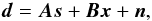 (2)where the
underlying microwave sky signal, s, is to be estimated. Here
A is the pointing matrix, which encodes how the sky is
scanned and n is a Gaussian, zero mean noise vector.
x denotes some extra instrumental effects, usually taken
hereafter to be constant baseline offsets, which we will use to model the correlated part
of the instrumental noise and B – a “pointing” matrix
for x describing how it is added to the time domain
data. Convolution with an instrumental beam, assumed here to be axially symmetric, is
already included in s.
(2)where the
underlying microwave sky signal, s, is to be estimated. Here
A is the pointing matrix, which encodes how the sky is
scanned and n is a Gaussian, zero mean noise vector.
x denotes some extra instrumental effects, usually taken
hereafter to be constant baseline offsets, which we will use to model the correlated part
of the instrumental noise and B – a “pointing” matrix
for x describing how it is added to the time domain
data. Convolution with an instrumental beam, assumed here to be axially symmetric, is
already included in s.
The signal part of the uncalibrated data vector, d, is the
detector response to the sky emission observed in the direction of
pixel p. For a total power detectors, e.g., the ones on
Planck, it is a linear combination of polarized and unpolarized
contributions:  (3)where it is implied that
sample t is measured in pixel p and
χt is a detector polarization angle with
respect to the polarization basis and we have dropped the baseline term for simplicity.
Equation (3) includes an overall
calibration factor 𝒦, and a cross polar leakage factor ϵ,
however, in what follows, we only consider the case of perfect calibration, setting
𝒦 = 1 with no loss of generality, and no leakage, ϵ = 0.
(3)where it is implied that
sample t is measured in pixel p and
χt is a detector polarization angle with
respect to the polarization basis and we have dropped the baseline term for simplicity.
Equation (3) includes an overall
calibration factor 𝒦, and a cross polar leakage factor ϵ,
however, in what follows, we only consider the case of perfect calibration, setting
𝒦 = 1 with no loss of generality, and no leakage, ϵ = 0.
To simplify future considerations we introduce a generalized pointing matrix,
A′, and a generalized map,
s′. They are defined as ![Mathematical equation: \begin{equation} \vec A' \equiv \left[ \vec A, \vec B\right], \mathrm{and} \, \vec s' \equiv \left[ \begin{array}{c} \vec s\\ \vec x \end{array} \right] \;\textrm{allowing us to write}\; \vec d = \vec A'\vec s' + \vec n. \label{eq:todprime} \end{equation}](/articles/aa/full_html/2010/14/aa12606-09/aa12606-09-eq29.png) (4)The detector
noise has a time-domain covariance matrix
𝒩 = ⟨ nnT ⟩
and the probability for the observed timeline, d, becomes
the Gaussian probability of a noise realization
n = d − A′s′:
(4)The detector
noise has a time-domain covariance matrix
𝒩 = ⟨ nnT ⟩
and the probability for the observed timeline, d, becomes
the Gaussian probability of a noise realization
n = d − A′s′:
![Mathematical equation: \begin{equation} \label{eq:map_prob} P(\vec d) = P(\vec n) = \left[(2\pi)^{\mathrm{dim}\,\vec n}\det\mathcal N\right]^{-1/2} \exp \left( -\frac{1}{2}{\vec n}^\mathrm T\mathcal N^{-1}\vec n \right) P\left(\vec x\right), \end{equation}](/articles/aa/full_html/2010/14/aa12606-09/aa12606-09-eq32.png) (5)where the last factor
is a prior constraint on the noise offsets, x, which
hereafter we will take to be a Gaussian with a zero mean and some correlation matrix,
𝒫, i.e.,
(5)where the last factor
is a prior constraint on the noise offsets, x, which
hereafter we will take to be a Gaussian with a zero mean and some correlation matrix,
𝒫, i.e.,  (6)By maximizing
this likelihood with respect to the sky signal and baselines contained
in s′, we find an expression for a maximum likelihood
estimate which reads,
(6)By maximizing
this likelihood with respect to the sky signal and baselines contained
in s′, we find an expression for a maximum likelihood
estimate which reads, ![Mathematical equation: \begin{equation} \label{eq:min_var_map} \hat{\vec s}'\! =\! \left( \mathcal R^{-1} + {\vec A'}^\mathrm T\mathcal N^{-1}\vec A' \right)^{-1}\!{\vec A'}^\mathrm T\mathcal N^{-1}\vec d, \, \textrm{where}\, \mathcal R^{-1} \equiv \left[ \begin{array}{c c} \vec 0 & \vec 0\\ \vec 0 & \mathcal P^{-1} \end{array} \right]. \end{equation}](/articles/aa/full_html/2010/14/aa12606-09/aa12606-09-eq35.png) (7)The first part of the
vector
(7)The first part of the
vector  is an
estimate of the actual sky signal, ,
while all the rest is an estimate of the baseline offsets,
is an
estimate of the actual sky signal, ,
while all the rest is an estimate of the baseline offsets,  .
The map
.
The map  is
called the noise-weighted map. In case of flat prior for x,
expressions identical to Eq. (7) can be
also derived from minimum variance or generalized least square considerations and we will
refer to as
either a minimum variance or optimal map in the future. We note that we have ignored here
any pixelization effects that cause differences between d
and A′s′ even for a noise-free
experiment. This is usually true in the limit of the pixel size significantly smaller than
the beam resolution of the instrument. If this condition is not fulfilled, the
pixelization effects may be important and special methods may be needed to minimize them.
We discuss specific proposals in Sect. 2.3. In the
absence of such effects, the difference between a map estimate, , and the
input map, s′, is called residual pixel domain
noise.
is
called the noise-weighted map. In case of flat prior for x,
expressions identical to Eq. (7) can be
also derived from minimum variance or generalized least square considerations and we will
refer to as
either a minimum variance or optimal map in the future. We note that we have ignored here
any pixelization effects that cause differences between d
and A′s′ even for a noise-free
experiment. This is usually true in the limit of the pixel size significantly smaller than
the beam resolution of the instrument. If this condition is not fulfilled, the
pixelization effects may be important and special methods may be needed to minimize them.
We discuss specific proposals in Sect. 2.3. In the
absence of such effects, the difference between a map estimate, , and the
input map, s′, is called residual pixel domain
noise.
Let us now consider first the prefactor matrix in Eq. (7),  (8)a weight matrix combining
both the baseline prior and the noise variance weights. It acts on the generalized
noise-weighted map, producing estimates of the pixels and baselines.
(8)a weight matrix combining
both the baseline prior and the noise variance weights. It acts on the generalized
noise-weighted map, producing estimates of the pixels and baselines.
Given that our generalized map is made of two parts: the actual sky signal and the
baseline offsets, the matrix M′ has four blocks: two
diagonal blocks, denoted M and
Mx, and two off-diagonal
blocks, each of which is a transposed version of the other and one of which is referred
here to as Mo. Using inversion by partition we
can write an explicit expression for each of these blocks. For example, for the sky-sky
diagonal blocks we get, ![Mathematical equation: \begin{eqnarray} \label{eq:MmatSS0} && \vec M \!=\! \left[\!\vec A^\mathrm T\mathcal N^{-1}\vec A \!-\!\left(\vec A^\mathrm T\mathcal N^{-1}\vec B\right)\! \left(\mathcal P^{-1}\!+\!\vec B^\mathrm T\mathcal N^{-1}\vec B\right)^{-1}\! \left(\vec A^\mathrm T\mathcal N^{-1}\vec B\right)^\mathrm T \right]^{-1}~~~~~~~~ \\ && \label{eq:MmatSS}\quad = \left(\vec A^\mathrm T\mathcal N^{-1}\vec A\right)^{-1} +\left(\vec A^\mathrm T\mathcal N^{-1}\vec A\right)^{-1} \left(\vec A^\mathrm T\mathcal N^{-1}\vec B\right)\nonumber\\ &&\qquad \qquad\times \vec M_ x \left(\vec A^\mathrm T\mathcal N^{-1}\vec B\right)^\mathrm T \left(\vec A^\mathrm T\mathcal N^{-1}\vec A\right)^{-1}, \end{eqnarray}](/articles/aa/full_html/2010/14/aa12606-09/aa12606-09-eq45.png) while
for the offset-offset part,
while
for the offset-offset part, ![Mathematical equation: \begin{eqnarray} \vec M_x &= & \bigg[ \mathcal P^{-1} + \vec B^\mathrm T\mathcal N^{-1}\vec B - \left(\vec B^\mathrm T\mathcal N^{-1}\vec A\right) \nonumber \\&& \times \left(\vec A^\mathrm T\mathcal N^{-1}\vec A\right)^{-1} \left(\vec B^\mathrm T\mathcal N^{-1}\vec A\right)^\mathrm T \bigg]^{-1}. \label{eq:MmatXX} \end{eqnarray}](/articles/aa/full_html/2010/14/aa12606-09/aa12606-09-eq46.png) (11)With
help of these equations we can now write explicit separate expressions for the estimated
sky signal and offsets. The former is given by,
(11)With
help of these equations we can now write explicit separate expressions for the estimated
sky signal and offsets. The former is given by,  (12)while the
latter,
(12)while the
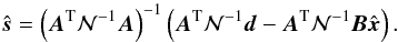
latter, 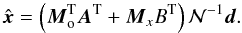 (13)We can also
combine these two equations to derive an alternative expression for the sky signal
estimate, which makes a direct use of the offsets assumed to be estimated earlier,
(13)We can also
combine these two equations to derive an alternative expression for the sky signal
estimate, which makes a direct use of the offsets assumed to be estimated earlier,
 (14)If the assumed
data model, Eq. (2), and the time domain
noise and baseline covariances are all correct, then the covariance of the residual pixel
domain noise is
(14)If the assumed
data model, Eq. (2), and the time domain
noise and baseline covariances are all correct, then the covariance of the residual pixel
domain noise is 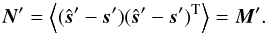 (15)In particular,
Eq. (1), the pixel-pixel residual noise
covariance matrix, N, is equal
to M and given by Eq. (10).
(15)In particular,
Eq. (1), the pixel-pixel residual noise
covariance matrix, N, is equal
to M and given by Eq. (10).
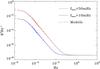 |
Fig. 1 Noise model (dashed lines) and the spectra of simulated noise (solid lines). The two sets of curves correspond to the two considered knee frequencies with fmin = 1.15 × 10⁻⁵ and α = 1.7. |
We note that a sufficiently high-quality estimate of the inverse time domain correlations, 𝒩-1, is required in order to calculate both the minimum-variance map and its noise covariance. If it is misestimated the map estimate will still be unbiased, though not any more minimum variance or maximum likelihood, and its covariance will not be given any more by Eq. (15).
For example for computational reasons we will find later that using some other matrix,
denoted here as ℳ-1, rather than the actual inverse noise covariance,
𝒩-1, in the calculation of the map estimates in Eq. (7) can be helpful. The corresponding noise
correlation matrix for such a map is then given by (Stompor et al. 2002, ungeneralized case) 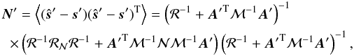 (16)where
ℳ and ℛ define our mapmaking operator, whereas 𝒩 and ℛ𝒩 are the
true noise properties. This expression is significantly more complex and computationally
involved than Eq. (15). Fortunately, as we
discuss in the following, in many cases of interest, the latter expression turns out to be
a sufficiently good approximation of the former with 𝒩-1 replaced by
ℳ-1 at least for some of the potential applications.
(16)where
ℳ and ℛ define our mapmaking operator, whereas 𝒩 and ℛ𝒩 are the
true noise properties. This expression is significantly more complex and computationally
involved than Eq. (15). Fortunately, as we
discuss in the following, in many cases of interest, the latter expression turns out to be
a sufficiently good approximation of the former with 𝒩-1 replaced by
ℳ-1 at least for some of the potential applications.
The mapmaking methods considered for Planck fall into two general
classes both of which are described by the equations derived above. The first class,
called optimal methods, assumes the sufficient knowledge of the time domain noise
correlations, does not introduce any extra degrees of freedom,
x, (or alternately assumes a prior for them with 𝒫
vanishing). In this case one can derive from Eqs. (14) and (10),
 where
the latter is a covariance of the residual noise of the former.
where
the latter is a covariance of the residual noise of the former.
The second class of methods introduces a number of baseline offsets with a Gaussian correlated (so-called generalized destripers) or uncorrelated (standard destripers) prior on them and describe the noise as an uncorrelated Gaussian process. The destriper maps are evaluated via Eq. (12) or Eq. (14), with 𝒩 assumed to be diagonal. Clearly on the time-domain level the destriper model is just an approximation, therefore at least a priori we should use the full expression in Eq. (16) to estimate its covariance. The CTP papers (Poutanen et al. 2006; Ashdown et al. 2007a,b, 2009) have shown that for Planck the two methods produce maps which are very close to one another. Moreover, they have shown that using a generalized destriper, the derived maps eventually become nearly identical to those obtained with the optimal methods, if an appropriate length of the baseline and a number of the baseline offsets is adopted together with a consistently evaluated prior. This motivates using the simplified Eq. (10) as an approximation for the noise covariance of the destriped maps, i.e., N = M. We will investigate the quality and applicability of this approximation later in this paper.
2.2. Time domain noise
We assume that the time domain noise is a Gaussian process and for the simulations we
take the noise power spectral density to have the form 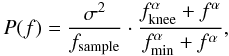 (19)where the shape is
defined by the slope, minimum and knee frequencies (α,
fmin and fknee respectively) and
the scaling by the white-noise sample variance and sampling frequency (σ
and fsample). Two examples of the theoretical and simulated
noise spectra can be seen in Fig. 1.
(19)where the shape is
defined by the slope, minimum and knee frequencies (α,
fmin and fknee respectively) and
the scaling by the white-noise sample variance and sampling frequency (σ
and fsample). Two examples of the theoretical and simulated
noise spectra can be seen in Fig. 1.
In the calculations of the maps using the optimal algorithms or generalized destripers we will assume that noise power spectrum is known precisely. As the noise simulated in the cases analyzed here is piece-wise stationary, with no correlations allowed between the data in the different pieces (see Sect. 5) the respective noise correlation matrix, 𝒩, is block Toeplitz with each of the blocks, describing the noise correlations of one of the stationary pieces, defined by the noise power spectrum. Given that we will approximate the inverse of 𝒩 as also a block Toeplitz matrix with each blocks given by an inverse noise power spectrum. Though this is just an approximation it has been demonstrated in the past that it performs exquisitely well in particularly in the cases with long continuous pieces of the stationary noise (Stompor et al. 2002), as it is a case in all simulations considered here.
2.3. Low-resolution maps
The high-resolution (down to ~5 arcmin) of the Planck data makes it impossible with current resources to evaluate and store the full pixel-pixel covariance of all map pixels. The solution is to produce a low-resolution dataset for the study of large scale structure of the microwave sky. Low-resolution mapmaking for a high-resolution mission is non-trivial for two reasons: first, the considered mapmaking methods assume that there exists no sky structure at the sub pixel scale. Secondly, cosmological information contained in the polarization signal has several orders of magnitude worse signal-to-noise ratio than intensity signal, causing completely different downgrading effects in the Stokes I, Q and U maps.
In this section we define three alternative methods of producing low-resolution maps from high-resolution observations. The first two, direct and (inverse) noise weighting methods, have already been used in the WMAP analysis (Jarosik et al. 2007). As the third option we consider smoothed (low-pass-filtered) maps and their noise covariance.
2.3.1. Direct method
The most straightforward method to produce a low-resolution map is to project the detector observations directly to the pixels of the final target resolution. Hereafter we will refer to it as the direct method.
Solving the low-resolution map directly involves less uncertainty. This means that the solved and subtracted correlated noise realization is more accurate. The absence of intermediate, high-resolution products makes noise in the direct maps easier to model. The noise covariance matrices for the direct maps can be computed using formalism presented in Sect. 2.1, for example, Eqs. (15) and (16).
On the other hand, if the sky signal varies within the pixels, non-uniform sampling of a pixel can cause a systematic error in the solved map (Ashdown et al. 2007a). This is an important aspect, as none of the considered algorithms deal with sub pixel structures by design.
In Sect. 6.3 we quantify the signal error for the different low-resolution maps and mapmakers.
Hereafter, we will use the direct method as a reference with respect to which we compare the other approaches.
2.3.2. Inverse noise weighting (INW)
In the case of nested pixelization schemes, such as Hierarchical Equal Area isoLatitude Pixelization (HEALPix, Górski et al. 2005) used in this paper, to downgrade a temperature only map, one may compute a weighted average of the sub pixel temperatures. A natural choice are the optimal, inverse noise weights that lead to minimum noise of the super pixel in the absence of correlated noise. We will refer to these maps as inverse noise weighted (INW) maps.
A similar weighting scheme exists for the polarized data as well. Algebraically, the
entire procedure can be summarized on the map level as,  (20)where
W and W′′ are weight
matrices for the high and low resolution maps, respectively. They depend on
A and A′′ – the pointing
matrices at high and low resolution. X simply sums the
pixels in resolution Npix to resolution
(20)where
W and W′′ are weight
matrices for the high and low resolution maps, respectively. They depend on
A and A′′ – the pointing
matrices at high and low resolution. X simply sums the
pixels in resolution Npix to resolution
 ,
,  (21)weights
are given by,
(21)weights
are given by,  (22)and
𝒩u is the time domain covariance matrix of the uncorrelated part of
the noise, n.
(22)and
𝒩u is the time domain covariance matrix of the uncorrelated part of
the noise, n.
The covariances for the maps obtained via such a procedure can be derived from Eq. (20) and the expressions described in Sect. 2.1.
Noise weighting reduces signal errors by first solving the map at a resolution where sub pixel structure is weak. In comparison to the direct method, the more accurate signal is gained at the cost of higher noise. Like the direct method, INW disregards any sub pixel structure but at high-resolution. In this case the instrument beam naturally smoothes out small scale structure causing the approximation to hold.
2.3.3. Harmonic smoothing
Both methods described above may result in the signal smoothing (or its band-width) being position-dependent as it is achieved via averaging of the observed high-resolution pixel amplitudes contained within each low-resolution pixel.
Applying a smoothing operator to the high-resolution map prior to resolution downgrading could alleviate such a problem. The smoothing operation needs to properly take care of the high frequency power contained in the maps, not to alias it as power at the scales of interest.
As the smoothing operation is usually performed in the harmonic domain, it requires that the high-resolution map is first expanded in spherical harmonics. If the sky is only partially covered, the expansion is not unique. Since Planck is a full sky experiment, we do not address the partial sky problem here but leave it for future work.
To suppress small angular scale power the expansion is convolved with an axially
symmetric window function (e.g. a symmetric Gaussian window function Challinor et al. 2000), ![Mathematical equation: \begin{eqnarray} \label{eq:beam_window} & & \tilde a^\mathrm T_{\ell m} = W_\ell a^\mathrm T_{\ell m}, W_\ell = {\rm e}^{-\frac{1}{2}\ell(\ell+1)\sigma^2} \\ & &\tilde a^\mathrm E_{\ell m} = {}_2W_\ell a^\mathrm E_{\ell m}, _2W_\ell = {\rm e}^{-\frac{1}{2}[\ell(\ell+1)-4]\sigma^2}, \end{eqnarray}](/articles/aa/full_html/2010/14/aa12606-09/aa12606-09-eq80.png) chosen
to leave only negligible power at angular scales that are not supported by the low
target resolution. Finally the regularized expansion is synthesized into a
low-resolution map by sampling the expansion values at pixel centers. We conduct most of
our studies using a beam having a full width at half maximum (FWHM) of
twice the average pixel side. For the Nside = 32
resolution2 this is approximately 220′
(
chosen
to leave only negligible power at angular scales that are not supported by the low
target resolution. Finally the regularized expansion is synthesized into a
low-resolution map by sampling the expansion values at pixel centers. We conduct most of
our studies using a beam having a full width at half maximum (FWHM) of
twice the average pixel side. For the Nside = 32
resolution2 this is approximately 220′
( ). Whenever transforms between harmonic and
pixel space are conducted, it is important to consider the range of multipoles included
in the transformation. We advocate using such an aggressive smoothing that the harmonic
expansion has negligible power beyond
ℓ = 3Nside and results are stable for any
ℓmax beyond this. For completeness we have set
ℓmax = 4Nside but stress that
any residual power beyond ℓ = 3Nside will
lead to aliasing.
). Whenever transforms between harmonic and
pixel space are conducted, it is important to consider the range of multipoles included
in the transformation. We advocate using such an aggressive smoothing that the harmonic
expansion has negligible power beyond
ℓ = 3Nside and results are stable for any
ℓmax beyond this. For completeness we have set
ℓmax = 4Nside but stress that
any residual power beyond ℓ = 3Nside will
lead to aliasing.
The smoothing window does not need to be a Gaussian but it is preferable to avoid sharp
cut-offs that may induce “ringing” phenomena. Benabed
et al. (2009) suggest a window function that preserves the signal basically
unchanged until a chosen threshold and then smoothly kills all power quickly above that
angular resolution. Their window is ![Mathematical equation: \begin{equation} \label{eq:teasingbeam} W_\ell = \left\{ \begin{array}{cl} 1, & \ell \leq \ell_1 \\ \frac{1}{2}\left[ 1+\cos\left((\ell-\ell_1)\pi/(\ell_2-\ell_1)\right)\right], & \ell_1 < \ell \leq \ell_2 \\ 0, & \ell > \ell_2 \end{array} \right. \end{equation}](/articles/aa/full_html/2010/14/aa12606-09/aa12606-09-eq87.png) (25)with
the typical choice
ℓ1 = 5Nside / 2 and
ℓ2 = 3Nside.
(25)with
the typical choice
ℓ1 = 5Nside / 2 and
ℓ2 = 3Nside.
In contrast to the two noise-driven methods, harmonic smoothing can be considered optimal from the (large-scale) signal viewpoint; however it may be suboptimal as far as the noise is concerned, in particular in the case of strongly inhomogeneous noise distribution.
The noise covariance matrices described in Sect. 2.1 need to be amended to accurately characterize the smoothed maps and thus
we need to smooth the matrices as well. Smoothing of a map is a linear operation. For
any linear operator, L, acting on a map,
m, we can compute its covariance as  (26)where
λi and
ei stand for eigenvalues
and eigenvectors of the noise covariance, N, i.e.,
(26)where
λi and
ei stand for eigenvalues
and eigenvectors of the noise covariance, N, i.e.,
 ,
and m is understood here to contain only noise. We
note that in general one should replicate the same processing steps for the covariance
matrix as are to be applied to maps and therefore the smoothing operation should be
applied to the noise covariance of the high-resolution map and its resolution downgraded
later.
,
and m is understood here to contain only noise. We
note that in general one should replicate the same processing steps for the covariance
matrix as are to be applied to maps and therefore the smoothing operation should be
applied to the noise covariance of the high-resolution map and its resolution downgraded
later.
In order to make the evaluation of Eq. (26) feasible, we must commute the order of the smoothing and downgrading operations contained in L. Though these two operations are clearly not exchangeable on the map level, due to the potential presence of the subpixel power, such an approach can be more justifiable for the noise covariances. In this case we can explicitly compute the low-resolution unsmoothed covariance matrices directly and subsequently smooth them with the signal smoothing kernel.
In the following we will apply the smoothing technique to both high and low resolution maps already downgraded using some of the other approaches. We will demonstrate that such a combined approach results in controllable properties of the residual noise on the one hand and well defined sky signal bandwidth on the other. Unlike both the direct and INW methods, the smoothed low-resolution maps are actually solved from a signal that lacks sub pixel structure.
3. Numerical calculations of residual noise covariance
This section presents numerical methods to compute the residual noise covariance matrix and describes briefly their implementations corresponding to three different mapmaking methods, the optimal method (MADping and ROMA implementations) and the generalized (Madam) and classical destriping (Springtide) methods.
3.1. Optimal map covariance
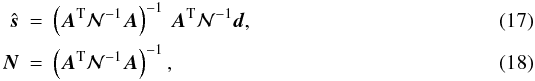
The noise covariance of optimal maps assuming exact noise model is given by Eq. (18). It is evaluated in two steps: first the inverse covariance matrix, AT𝒩-1A, is assembled and subsequently inverted. Given that the matrix can be singular the latter step may require computing the pseudo-inverse.
The pseudo-inverse is defined by the eigenvalue decomposition of the inverse noise
matrix. Because the noise matrix is symmetric and, by definition, non-negative definite,
its eigenvalues are real and non-negative
(λi ≥ 0), and its eigenvectors form a
complete orthogonal basis. This allows us to expand the matrix as  (27)Here
λi are the eigenvalues and
(27)Here
λi are the eigenvalues and
 are the
corresponding eigenvectors of the matrix N-1. We
can now invert N-1 by using its eigenvalue
decomposition,
are the
corresponding eigenvectors of the matrix N-1. We
can now invert N-1 by using its eigenvalue
decomposition,  (28)and controlling the
ill-conditioned eigenmodes. Any ill-conditioned eigenmode will have an eigenvalue several
orders of magnitude smaller than the largest eigenvalue. By including in the sum only the
well-conditioned eigenmodes we effectively project out the correlation patterns that our
methods cannot discern.
(28)and controlling the
ill-conditioned eigenmodes. Any ill-conditioned eigenmode will have an eigenvalue several
orders of magnitude smaller than the largest eigenvalue. By including in the sum only the
well-conditioned eigenmodes we effectively project out the correlation patterns that our
methods cannot discern.
We describe in Sect. A.3, that the covariance is indeed commonly expected to be singular or nearly so.
MADping is one of the codes of the MADCAP3 suite of
CMB analysis tools (Borrill 1999). In this
implementation, each processor scans through its sections of time-ordered data and
accumulates its local piece of the inverse noise covariance. These pieces are then
gathered and written to disk. The scaling of this technique is 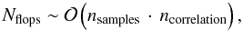 (29)where
ncorrelation is the filter length set by the noise
autocorrelation length.
(29)where
ncorrelation is the filter length set by the noise
autocorrelation length.
For a Planck-sized, full-sky dataset and using a reasonable pixel
resolution (half a degree), the construction of the inverse noise covariance dominates
over the computational cost of inverting this matrix. Nevertheless, inversion methods as
well as the eigendecomposition scale as  .
.
In order to correctly treat the signal component of the data map in Eq. (7), we must apply our low-resolution noise covariance to a noise-weighted map which has been downgraded from higher resolution. This downgrading process is equivalent to the technique discussed in Sect. 2.3.2, and ensures that signal variations inside a low-resolution pixel are accounted for. The high-resolution noise-weighted map consistent with the above formalism is constructed as the first step of the mapmaking carried out by the MADmap program (Cantalupo et al. 2010). The matrix eigenvalue decomposition is done using a ScaLAPACK4 interface that allows efficient parallel eigenvalue decomposition of large matrices using a divide-and-conquer algorithm.
The ROMA code (Natoli et al. 2001; de Gasperis et al. 2005) is an implementation of the
optimal generalized least squares (GLS) iterative map making specifically designed for
Planck, but also successfully used on suborbital experiments such as
BOOMERanG (Masi et al. 2006). To estimate noise
covariance as in Eq. (15) we start by
calculating row i of its inverse,
N-1, by computing its action on the unit vector
along axis i: 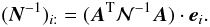 (30)This calculation is
implemented as follows: i) projecting the unit vector into a TOD by applying
A on ; ii)
noise-filtering the TOD in Fourier space; iii) projecting the TOD into a map by applying
AT. By computing each column independently we
reduce memory usage because we allocate memory only for one map instead of allocating
memory for the full matrix. The computational cost of the full calculation is dominated by
Fourier transforms that are repeated as many times as the number of columns, hence the
scaling can be expressed as:
(30)This calculation is
implemented as follows: i) projecting the unit vector into a TOD by applying
A on ; ii)
noise-filtering the TOD in Fourier space; iii) projecting the TOD into a map by applying
AT. By computing each column independently we
reduce memory usage because we allocate memory only for one map instead of allocating
memory for the full matrix. The computational cost of the full calculation is dominated by
Fourier transforms that are repeated as many times as the number of columns, hence the
scaling can be expressed as: 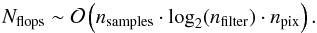 (31)Alternately, we can
compute the NCM column-by-column with help of multiple mapmaking-like operations, i.e.,
(31)Alternately, we can
compute the NCM column-by-column with help of multiple mapmaking-like operations, i.e.,
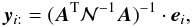 (32)where
 is a unit
vector as defined above and yi
stands for a column of N. We rewrite the above equation as
is a unit
vector as defined above and yi
stands for a column of N. We rewrite the above equation as
 (33)and solve it using the
standard PCG mapmaking solver. In such case there is no need to store a full inverse noise
covariance matrix in the memory of a computer at any single time as the operations on the
lhs can be performed from right to left. As a result, this approach can be
applied also for high-resolution cases for which the direct method described above would
not be feasible.
(33)and solve it using the
standard PCG mapmaking solver. In such case there is no need to store a full inverse noise
covariance matrix in the memory of a computer at any single time as the operations on the
lhs can be performed from right to left. As a result, this approach can be
applied also for high-resolution cases for which the direct method described above would
not be feasible.
We note that unlike in the previous approaches based on the direct matrix inversion in the latter case there is no special care taken of potential singularities. Though the presence of those does not hamper the PCG procedure (e.g., Cantalupo et al. 2010), nonetheless care must be taken while interpreting its results.
3.2. Destriped map covariance
In the destriping approach to mapmaking, we model all noise correlations by baseline
offsets. Thus we write Eq. (2) as
 (34)where
nu is a vector of uncorrelated white noise
samples. Accordingly, we must replace the time-domain noise covariance matrix, 𝒩,
by a diagonal matrix, 𝒩u. All noise correlation is then included in the
prior baseline offset covariance matrix, 𝒫.
(34)where
nu is a vector of uncorrelated white noise
samples. Accordingly, we must replace the time-domain noise covariance matrix, 𝒩,
by a diagonal matrix, 𝒩u. All noise correlation is then included in the
prior baseline offset covariance matrix, 𝒫.
If we now apply the destriping approximation to Eqs. (9) we find for the pixel-pixel residual noise covariance matrix:
 (35)The first term on
the rhs is the binned white noise contribution (a diagonal or block-diagonal
matrix for temperature-only and polarized cases respectively) and the second term
describes the pixel-pixel correlations due to errors in solving for the baselines, i.e.,
the difference between the solved and actual baselines (Kurki-Suonio et al. 2009).
(35)The first term on
the rhs is the binned white noise contribution (a diagonal or block-diagonal
matrix for temperature-only and polarized cases respectively) and the second term
describes the pixel-pixel correlations due to errors in solving for the baselines, i.e.,
the difference between the solved and actual baselines (Kurki-Suonio et al. 2009).
When making a map using destriping, one can use high resolution to solve for baselines and still bin the map at low resolution. Since this is equivalent to producing first a high-resolution map and then downgrading through inverse noise weighting, we will always assume the same pixel size for both of these steps.
3.2.1. Conventional destriping
Springtide (Ashdown et al. 2007b) is an
implementation of the conventional destriping approach which solves for one baseline per
pointing period. Since the baselines are so long, it allows for a number of
optimizations in the handling of the data. During one pointing period, the same narrow
strip of sky is observed many times, so the time-ordered data are compressed into rings
before doing the destriping. Another effect of the long baselines is that the prior
covariance matrix of the baselines, 𝒫, is strongly diagonal-dominant, so to a
very good approximation can be assumed to be diagonal. As a consequence, the matrix
 that appears in the expression for the inverse map covariance matrix (35) is also diagonal. Thus the number of
operations taken to compute (35) is
that appears in the expression for the inverse map covariance matrix (35) is also diagonal. Thus the number of
operations taken to compute (35) is
 (36)The number of
baselines is small compared to the generalized destriping approach, so it is also
possible to compute the inverse posterior covariance matrix of the baseline offsets
explicitly, invert it and use it to compute the map covariance matrix. This method has
the advantage that the resolution at which the destriping is performed is not
constrained to be the same as the resolution of the final map covariance matrix. The
destriping can instead be done at the natural resolution of the data to avoid subpixel
striping effects. The inverse of the posterior baseline error covariance matrix can be
calculated using Eq. (11) and the
corresponding map covariance matrix is given by Eq. (10). However, the pointing matrices, A,
need not be for the same resolution in both steps.
(36)The number of
baselines is small compared to the generalized destriping approach, so it is also
possible to compute the inverse posterior covariance matrix of the baseline offsets
explicitly, invert it and use it to compute the map covariance matrix. This method has
the advantage that the resolution at which the destriping is performed is not
constrained to be the same as the resolution of the final map covariance matrix. The
destriping can instead be done at the natural resolution of the data to avoid subpixel
striping effects. The inverse of the posterior baseline error covariance matrix can be
calculated using Eq. (11) and the
corresponding map covariance matrix is given by Eq. (10). However, the pointing matrices, A,
need not be for the same resolution in both steps.
The structure of the inverse posterior baseline covariance matrix, Eq. (11), depends on the scanning strategy, but it is in general a dense matrix. Inverting the matrix and using it to compute Eq. (10) involves dense matrix operations, so this method is computationally more demanding than the other approach described above. However, the posterior baseline covariance matrix needs only to be computed once and stored, and then can be used many times to compute the map covariance matrix for any desired resolution. It is also possible to use Eq. (10) to compute the residual noise covariance matrix for a subset of the pixels in the map.
3.2.2. Generalized destriping
Madam (Keihänen et al. 2005, 2010) is an implementation of the generalized destriping principle. It is flexible in the choice of baseline length and makes use of prior information of baseline covariance (𝒫 is not approximated to be diagonal).
Even for a generalized destriper, all the matrices in Eq. (35) are extremely sparse. Most of the
multiplications only require operations proportional to the number of pixels, baselines
or samples. The matrices 𝒫-1 and
are approximately circulant, band-diagonal matrices whose width is determined by the
noise spectrum. For all cases studied in this paper, the latter matrix is limited to the
order of 103 non-negligible elements per row. We call this width the
baseline correlation length, ncorr.
ncorr corresponds to a few hours of samples and is
inversely proportional to baseline length, nbl. In addition
to the correlated noise part, our formalism naturally includes pixel correlations due to
white noise.
We evaluate the prior baseline offset matrix from the power spectral density (PSD) of
the correlated noise, P(f), by Fourier transforming
the baseline PSD, Px(f),
into the autocorrelation function. The baseline PSD is evaluated as (Keihänen et al. 2010): 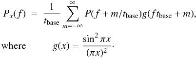 (37)The
sum converges after including only a few m around the origin. For
stationary noise, any row of 𝒫-1 can then be evaluated as a cyclic
permutation of
ℱ-1 [ 1 / Px(f) ] .
(37)The
sum converges after including only a few m around the origin. For
stationary noise, any row of 𝒫-1 can then be evaluated as a cyclic
permutation of
ℱ-1 [ 1 / Px(f) ] .
We evaluate (35) after computing (37) by approximating the inner matrix,
,
as circulant. This allows us to invert the
nbase × nbase band diagonal
matrix by two short Fourier transforms. It turns out that the matrix multiplications are
most conveniently performed by first evaluating the sparse  matrix and then operating with it on the inner matrix from both sides.
Actually the inverse covariance matrix gains a contribution from all quadruplets
(xi,xj,p,q),
where baselines xi and
xj are within baseline
correlation length and hit pixels p and q. The number
of operations required to complete the estimate is then proportional to 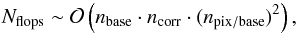 (38)where
nbase and ncorr, the number of
baselines per survey and correlation length respectively, are inversely proportional to
the length of a baseline. In contrast, npix / base, pixels
per baseline, is proportional to baseline length. For short baselines and low-resolution
maps, the magnitude of npix / base is close to unity.
Table 1 lists low-resolution
Nside parameters and the baseline lengths that correspond
to average pixel sizes. It can be used to estimate
npix / base and shows that, for example, 1.25s baseline
offset at Nside = 32 resolution covers approximately
4 pixels. The success of this approach is to replace the number of baselines squared,
(38)where
nbase and ncorr, the number of
baselines per survey and correlation length respectively, are inversely proportional to
the length of a baseline. In contrast, npix / base, pixels
per baseline, is proportional to baseline length. For short baselines and low-resolution
maps, the magnitude of npix / base is close to unity.
Table 1 lists low-resolution
Nside parameters and the baseline lengths that correspond
to average pixel sizes. It can be used to estimate
npix / base and shows that, for example, 1.25s baseline
offset at Nside = 32 resolution covers approximately
4 pixels. The success of this approach is to replace the number of baselines squared,
 , in the computation
complexity by
, in the computation
complexity by  .
.
Pixel side to baseline length at 1 rpm spin rate.
3.3. Smoothed covariance matrices
We define the linear smoothing operator, L, of Eq. (26) as
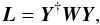 (39)where each row of
the matrix Y is a map of the relevant spin-0 and spin-2
spherical harmonic functions. Y acts on a map vector and
returns its spherical harmonic expansion:
a = Ym.
W is the smoothing kernel matrix that suppresses power
at the chosen scales according to Eq. (23).
(39)where each row of
the matrix Y is a map of the relevant spin-0 and spin-2
spherical harmonic functions. Y acts on a map vector and
returns its spherical harmonic expansion:
a = Ym.
W is the smoothing kernel matrix that suppresses power
at the chosen scales according to Eq. (23).
The smoothing procedure on its own will often lead to singular eigenvectors of the smoothed covariance matrix, with the eigenvalues corresponding to those close to zero. Though at a first glance such eigenvectors may look like being strongly constrained by the data, their actual value in the analysis is negligible as the sky signal in those modes is also smoothed. The nearly vanishing variance of those modes will often spuriously exaggerate the smoothing and mapmaking artifacts likely present whenever any inverse noise weighting needs to be applied. To avoid such problems hereafter we apply the pseudo-inverse described in 3.1 The criterion for selecting the nearly singular modes will in general depend on the case at hand and we will discuss the matter with the χ2 test in Sect. 6.2.
In some cases the eigenvalue decomposition of the smoothed matrix may not be readily
available or its computation not desirable. We can then regularize the inversion
of  by adding some low level of the pixel-independent uncorrelated noise. For consistency, a
random realization of such noise should also be added to the corresponding maps. We note
that both approaches are effectively equivalent and that the choice of the singularity
threshold needed to select the singular eigenmodes corresponds roughly to the choice of
the noise level to be added. We will commonly use the latter approach in some of the power
spectrum tests discussed later.
by adding some low level of the pixel-independent uncorrelated noise. For consistency, a
random realization of such noise should also be added to the corresponding maps. We note
that both approaches are effectively equivalent and that the choice of the singularity
threshold needed to select the singular eigenmodes corresponds roughly to the choice of
the noise level to be added. We will commonly use the latter approach in some of the power
spectrum tests discussed later.
4. Numerical tests and comparison metric
This paper has two main goals. On the one hand we propose and compare various methods devised to produce the low-resolution maps, searching for the mapmaking method which leads to low-resolution maps virtually free of artifacts such as those due to subpixel power aliasing. In parallel we develop the tools to estimate residual noise covariance for such maps, which properly describe the error of the estimated maps due to residual noise. The numerical results presented in the subsequent sections of the paper aim therefore at comparing and validating the algorithms which we have presented earlier. The discussed comparisons involve standard statistical tests, such Kolmogorov-Smirnov, χ2, etc. and ones which are specifically devised in the light of the anticipated future applications of the maps and their covariances. We describe such tests in this section.
4.1. Quadratic maximum likelihood power spectrum estimation
One of the main applications for the low-resolution noise covariance matrices we envisage is to the estimation of power spectra, Cℓ. This is often separated into the estimation of large and small angular scales, usually associated with high and low signal to noise regimes. The methods discussed here are relevant for large angular scales. The successful estimation of the underlying true power spectrum of the sky signal sets demanding requirements for the quality of the maps produced for such a purpose as well as the consistency of the estimated noise covariance and the actual noise contained in the map. For this reason we will use hereafter power spectrum estimation as one of the metrics with which to evaluate the quality of the proposed algorithms.
We will use the quadratic maximum likelihood (QML) method for the power spectrum
estimation as introduced in (Tegmark 1997) and
later extended to polarization in (Tegmark &
de Oliveira-Costa 2001). Given a temperature and polarization map,
m, the QML provides estimates of the power spectra, that
read, ![Mathematical equation: \begin{equation} \hat{C}_\ell^X = \sum_{\ell' , X'} (\vec F^{-1})^{X \, X'}_{\ell\ell'} \left[ \vec m^\mathrm T\vec E^{\ell'}_{X'}\vec m -\mathrm{tr}(\vec N{\vec E}^{\ell'}_{X'}) \right]. \label{eq:QMLestim} \end{equation}](/articles/aa/full_html/2010/14/aa12606-09/aa12606-09-eq155.png) (40)Here,
(40)Here,
 is an estimated power
spectrum, X = TT,EE,TE,BB,TB, or EB, and
is an estimated power
spectrum, X = TT,EE,TE,BB,TB, or EB, and  is the Fisher matrix. F and E
are defined as
is the Fisher matrix. F and E
are defined as ![Mathematical equation: \begin{equation} \vec F^{\ell\ell'}_{X X'} =\frac{1}{2}\mathrm{tr}\Big[{\vec C}^{-1}\frac{\partial {\vec C}}{\partial C_\ell^X}{\vec C}^{-1}\frac{\partial {\vec C}}{\partial C_{\ell'}^{X'}}\Big] \; \textrm{and} \; \vec E^\ell_X =\frac{1}{2}{\vec C}^{-1}\frac{\partial\vec C}{\partial C_\ell^X}\vec C^{-1}, \label{eq:QMLelle} \end{equation}](/articles/aa/full_html/2010/14/aa12606-09/aa12606-09-eq162.png) (41)where
C = S(Cℓ) + N
is the (signal plus noise) covariance matrix of the map, m.
Cℓ is a fiducial power spectrum needed for
the calculation of the signal part of the covariance. In this paper we will take it to be
given by the true power spectrum as used to produce the simulated skies. Though this would
be an unfair assumption, while testing the performance of this power spectrum estimation
technique, it is justified in our case, where the fact that it leads to the minimal
estimation uncertainties increases the power of our test.
(41)where
C = S(Cℓ) + N
is the (signal plus noise) covariance matrix of the map, m.
Cℓ is a fiducial power spectrum needed for
the calculation of the signal part of the covariance. In this paper we will take it to be
given by the true power spectrum as used to produce the simulated skies. Though this would
be an unfair assumption, while testing the performance of this power spectrum estimation
technique, it is justified in our case, where the fact that it leads to the minimal
estimation uncertainties increases the power of our test.
Gruppuso et al. (2009) describe a specific implementation of the QML method, nicknamed Bolpol, used in this work and discusses its performance in the application to the WMAP 5 year data. The QML estimator is known to be equivalent to a single iteration of a quasi-Newton-Raphson procedure to search for the true likelihood maximum (Bond et al. 1998).
Frequently used symbols in this paper.
4.2. Noise bias
In the mapmaking methods considered in this paper residual noise in the maps is independent of the sky properties and completely defined by the time-domain noise properties and the scanning strategy. The noise present in the maps contributes to the power spectrum estimates of the map signal. We will therefore refer to this contribution as the noise bias and use it to quantify the noise level expected in the maps of our different methods in a manner more succinct and manageable than the full noise covariance.
The noise bias is defined to be the expectation value for angular power spectrum in the
noise-only case 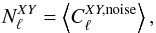 (42)where
X and Y stand for T, E and B. In the general case of a
quadratic estimator, such as QML, Eq. (40), the power spectrum estimates are given as a quadratic form of the input map,
m,
(42)where
X and Y stand for T, E and B. In the general case of a
quadratic estimator, such as QML, Eq. (40), the power spectrum estimates are given as a quadratic form of the input map,
m, 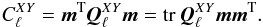 (43)By taking
m to be noise-only, the noise bias can be expressed as
(43)By taking
m to be noise-only, the noise bias can be expressed as
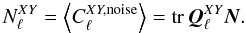 (44)Given the
eigenvalue decomposition of the noise covariance matrix,
(44)Given the
eigenvalue decomposition of the noise covariance matrix,  , we can evaluate
the noise bias as
, we can evaluate
the noise bias as 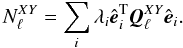 (45)In the following we
will validate the noise covariance matrices, estimated for the recovered sky maps, with
the help of their respective noise biases, which we will compare to results of Monte Carlo
simulations. In this context it is particularly useful to consider a
pseudo-Cℓ estimator that assumes uniform
pixel weights and full sky. For this estimator, the operator
(45)In the following we
will validate the noise covariance matrices, estimated for the recovered sky maps, with
the help of their respective noise biases, which we will compare to results of Monte Carlo
simulations. In this context it is particularly useful to consider a
pseudo-Cℓ estimator that assumes uniform
pixel weights and full sky. For this estimator, the operator  is
is 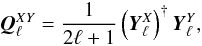 (46)where
 has
2ℓ + 1 rows that are maps of the appropriate spherical harmonics. It
maps a map vector into a vector of spherical harmonic expansion coefficients
has
2ℓ + 1 rows that are maps of the appropriate spherical harmonics. It
maps a map vector into a vector of spherical harmonic expansion coefficients
 where
m = − ℓ...ℓ.
where
m = − ℓ...ℓ.
The procedure we implement here involves two steps. First for every estimated noise
covariance we compute analytically the noise bias using Eqs. (45) and (46). Second, we compute the bias using Monte Carlo realizations of the
noise-only maps produced using the corresponding mapmaking procedure. The multiplications
 are conveniently implemented
using the HEALPix (Górski et al. 2005) Fortran 90
subroutine map2alm. We note that as we consider hereafter only full-sky cases, the noise
biases we compute as described above would be equal to those expected in the Maximum
Likelihood estimates of the sky power spectrum, were it not for the imperfection of the
sky quadrature due to pixelization effects (Górski et al.
2005).
are conveniently implemented
using the HEALPix (Górski et al. 2005) Fortran 90
subroutine map2alm. We note that as we consider hereafter only full-sky cases, the noise
biases we compute as described above would be equal to those expected in the Maximum
Likelihood estimates of the sky power spectrum, were it not for the imperfection of the
sky quadrature due to pixelization effects (Górski et al.
2005).
5. Simulation
5.1. Scanning strategy
In this study the Planck satellite orbits around the second Lagrangian
point (L2) of the Earth-Sun system (Dupac & Tauber
2005). The spin axis lies near the ecliptic plane, precessing with a six month
period around the anti-Sun direction at an angle of  . The focal plane
line-of-sight forms an 85° angle with the spin axis. In addition to these modes, we
include a nutation of the spin axis and slight variations to the 1rpm spin rate. Details
of the scanning simulation can be found from Ashdown et al.
(2009) where it was used in a mapmaking study.
. The focal plane
line-of-sight forms an 85° angle with the spin axis. In addition to these modes, we
include a nutation of the spin axis and slight variations to the 1rpm spin rate. Details
of the scanning simulation can be found from Ashdown et al.
(2009) where it was used in a mapmaking study.
5.2. Planck detectors
In this paper we study residual noise in the Planck 70 GHz frequency
maps. Planck has twelve detectors at 70 GHz. In the focal plane they are
located behind six horn antennas, a pair of detectors (“Side” and “Main” detectors5) sharing a horn. A pair of detectors measures two
orthogonal linear polarizations. The horns are split in two groups (three horns in a
group). The Side and Main polarization sensitive axes of a group are nearly aligned and
the polarization directions of the second group differ from the first group nominally
by 45°. Two horns from the different groups make a polarization pair that follows the same
scan path in the sky (three pairs in total with slightly different scan paths). As a
minimum the observations of a polarization pair are required to build a polarization map.
Due to implementation restrictions the Side and Main polarization axes are not fully
orthogonal and the polarization direction differences between the groups are not
exactly 45°, but the deviations from these nominal values are small
( ≲  ). The Side polarization axes of the two groups
differ by
). The Side polarization axes of the two groups
differ by  and
and  from the scan direction.
The beams of the detectors were assumed circularly symmetric with a 14′FWHM beam width. The beams do not impact the residual noise maps or covariance matrices. None of the mapmaking methods studied here make an attempt to correct for beam effects in the maps.
5.3. Time-ordered data
We computed the NCM’s of our three mapmaking methods using our noise model spectrum and the one year pointing data of twelve 70GHz detectors. We produced NCM’s for both Nside = 8 and Nside = 32 pixel sizes. We wanted to compare these NCM’s to the noise maps made by the same mapmaking methods. For that purpose we simulated 50 noise-only timelines and made maps from them. Our correlated noise streams were simulated in six day chunks by inverse Fourier transforming realizations of the noise spectrum (Natoli et al. 2002). We assumed an independence between the chunks and between the detectors. Figure 1 contains a comparison between the power spectra of the generated noise streams and the model spectra.
Twenty-five of the surveys featured a relatively high 1 / f contribution having the knee frequency, fknee, set to 50mHz. The other half was simulated to have a more favorable fknee = 10mHz. It should be noted that these frequencies have been chosen above and below the satellite spin frequency, 1rpm ≈ 17mHz. The slope of the 1 / f noise power spectrum was α = − 1.7. The correlation timescale of the 1 / f noise was restricted to about one day. This made our noise spectrum flat at low frequencies (below a minimum frequency fmin = 1.15 × 10⁻⁵Hzt1 / 24h). As we described earlier, it is the minimum frequency that determines the correlation length of the noise filter in the optimal mapmaking. In the noise covariance matrix of the generalized destriping, the baseline correlation length is, however, determined by the knee frequency.
We used a uniform white noise equivalent temperature (NET) of  for all detectors6. We chose this NET because we
wanted to produce noise maps and covariance matrices whose noise levels are compatible
with another CTP study (Jaffe et al., in prep.). In all mapmaking and NCM computations we
assumed a perfect knowledge of the detector noise spectrum.
for all detectors6. We chose this NET because we
wanted to produce noise maps and covariance matrices whose noise levels are compatible
with another CTP study (Jaffe et al., in prep.). In all mapmaking and NCM computations we
assumed a perfect knowledge of the detector noise spectrum.
The noise timelines were processed directly into both low-resolution (Nside = 32) and high-resolution (Nside = 1024) HEALPix maps using the discussed mapmaking codes. In the Nside = 1024 temperature and polarization maps the mean standard deviations of white noise per map pixel were 44 and 63μK (Rayleigh-Jeans μK). For Nside = 32 maps the corresponding values were 1.4 and 2.0μK.
The high-resolution maps were in turn downgraded to the low target resolution using the schemes detailed in Sect. 2.3.
For the signal error studies described in Sect. 6.3, we scanned simulated foreground maps into signal-only timelines. These we processed into low-resolution (Nside = 8) maps using the same methods as for the Nside = 32 (both directly and through high resolution). We then extracted the signal error part by subtracting a binned map from the destriped map. The foreground signal errors were summed with a CMB map to provide a worst case scenario of signal striping in otherwise perfectly separated CMB map.
5.4. Input maps
To study bandwidth limitation with respect to downgrading we simulated 117 high-resolution Nside = 1024 CMB skies corresponding to the same theoretical spectrum, Cℓ. These maps were smoothed and downgraded to Nside = 8 using three different Gaussian beams of widths 5°, 10°, 20° and three apodized step functions with the choices of (ℓ1,ℓ2) being (20,24), (16,24) and (16,20). A seventh set of downgraded maps was produced by noise weighting according to the scanning strategy. To comply with this last case, the smoothing windows include also the Nside = 8 pixel window function from the HEALPix package.
For the signal error exercise we used the Planck sky model, PSM7 version 1.6.3, to simulate the full microwave sky at 70GHz. For diffuse galactic emissions we included thermal and spinning dust, free-free and synchrotron emissions. We then added a Sunyaev-Zeldovich map and finally completed the sky with radio and infrared point sources. The combined Nside = 2048 map was smoothed with a symmetric Gaussian beam and scanned into a timeline according to the scanning strategy.
For final validation the noise covariance matrices were tested in power spectrum estimation. Each noise map was added to a random CMB map drawn from the theoretical distribution defined by a fixed theoretical CMB spectrum. The theoretical spectrum is the WMAP first-year best fit spectrum and has zero BB mode.
All maps in this work are presented in the ecliptic coordinate system. This choice is useful for Planck analysis since the scanning circles and many mapmaking artifacts form circles that connect the polar regions of the map. In this coordinate system the galaxy is not positioned at the equator but rather forms a downward opening horse shoe shape around the center of the map.
6. Results
In this section we first focus on the noise covariance matrices computed using different mapmaking techniques. We discuss and compare the overall noise patterns implied by such matrices and test the quality of the destriper approximation as applied to the noise covariance predictions. In the second part of the section we discuss the low-resolution maps and evaluate their quality in the light of their future potential applications, such as those to the large angular scale power spectrum estimation. Due to the computational resource restrictions the low-resolution results presented here are obtained either with the HEALPix Nside = 8 – in particular tests in Sect. 6.3 and power spectrum estimation tests in Sect. 6.2.3 – or Nside = 32 – in most of the other sections.
6.1. Noise covariance matrices
First we discuss the noise covariance matrices computed for the low-resolution maps of the direct method. As explained in Sect. 2.3 we compute from these matrices the noise covariances of the other downgrading techniques. In the following we consider noise covariance calculated using 4 different ways. In the first way we compute the noise covariance using the optimal algorithm. For this purpose we have developed two codes MADping or ROMA, which are described in Sect. 3.1. However, as they are just two different implementations of the same algorithm, we derive most of the results presented in the following and involving the optimal covariance using MADping. We note that whenever results from the both codes are available they have turned out to be virtually identical within the numerical precision expected from this kind of calculations. The optimal noise covariance matrices are expected to provide an accurate description of the noise level found in the actual optimal maps. We will test this expectation in the following and use the optimal results as a reference with which to compare the destriping results.
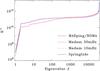 |
Fig. 2 Eigenspectra of the inverse covariance matrices N-1. MADping, ROMA and Madam results for fknee = 50mHz overlap completely. Springtide results are for 10mHz. |
The three remaining computations of the noise covariance are based on the destriping approach and correspond to different assumptions about the offset prior as well as baseline length. We consider the following specific cases: a classical destriper calculation with a baseline of 3600s (Springtide) and two generalized destriper computations with a baseline of 1.25 s and 60s (Madam). For each of these cases we will compare the covariance matrices with each other, with the optimal covariances and then test their consistency with the noise found in the simulated maps. We note again that this last property is not any more ensured given the approximate character of the destriper approach.
Figure 2 shows the eigenvalue spectra of some inverse NCMs. We note that all matrices possess a positive semi-definite eigenspectrum as is required for any covariance matrix, yet at the same time they all have one nearly ill-conditioned eigenmode8, which renders the condition number, i.e., the ratio of the largest and smallest eigenvalue, very large. This is in agreement with our expectations as described in Sect. A.3. Indeed the peculiar eigenmodes corresponding to the smallest eigenvalues of the inverse matrices are also found to be non-zero and constant for the I part of the vector and nearly zero for its polarized components, and thus close to the global offset vector discussed in Sect. A.3. The small deviations, on the order of 10-3, exist, as expected, as none of the peculiar modes is in fact truly singular. We note that the MADping and ROMA results, both computed in this test, are seen in the figure to be indistinguishable. They also coincide very closely with the Madam results computed for the same fknee = 50 mHz. The Springtide results, computed with fknee = 10 mHz are close to, though not identical with, the Madam results for the very same value of fknee when a longer (60s) baseline is used for Madam.
Figure 3 depicts the estimated
Stokes I, Q and U pixel variances as
well as the covariance between them. These quantities are dominated by the white noise
contribution and all methods describe white noise in the same manner. The top right-most
panel shows the reciprocal condition number (1/condition number) of the 3 × 3 blocks of
the matrix  for
each of the sky pixels. These numbers define our ability to disentangle the three Stokes
parameters for each of the pixels. Whenever they are equal to 1 / 2 not only can the
parameters be determined but their uncertainties will not be correlated. If the reciprocal
condition number for a selected pixel approaches 0, the Stokes parameters can not be
constrained. In the cases considered here, the Stokes parameters can clearly be determined
for all the pixels.
for
each of the sky pixels. These numbers define our ability to disentangle the three Stokes
parameters for each of the pixels. Whenever they are equal to 1 / 2 not only can the
parameters be determined but their uncertainties will not be correlated. If the reciprocal
condition number for a selected pixel approaches 0, the Stokes parameters can not be
constrained. In the cases considered here, the Stokes parameters can clearly be determined
for all the pixels.
Figure 3 shows a strong asymmetry between the IQ and IU blocks. The fact that the polarization axes of the two detectors of a horn are not fully perpendicular makes the I noise of a pixel correlate with the Q and U noises of the same pixel. We can imagine an instrument basis, where one group of three horns measures the Q of this basis and the other group measures the U of the same basis. Because Side and Main polarization axis deviations from the orthogonality have similar magnitudes in the two groups, we expect the diagonals of IQ and IU blocks to be similar (symmetric in IQ and IU) in the instrument basis. In the map we use a different polarization basis9. Building the noise weighted map (in the mapmaking) rotates the Q and U from the instrument basis to the map basis. The IQ and IU blocks become asymmetric in this rotation.
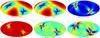 |
Fig. 3 Top: MADping pixel variances for temperature and polarization and the reciprocal condition number of the pixel observation matrices. Bottom: correlation coefficient × 103 between I − Q, I − U and Q − U pixels. This part of the noise covariance is dominated by white noise which is modeled equivalently in all three paradigms. Hence, MADmap, ROMA, Madam and Springtide results are nearly identical. Maps are rotated into galactic coordinates to show the structure near the ecliptic poles. |
 |
Fig. 4 A single column of the MADping covariance matrix corresponding to a pixel at the ecliptic equator. For both ROMA and Madam 1.25s baseline counterparts all visible characteristics remain unchanged. We plot the value of the correlation coefficient, R, multiplied by 103. In order to enhance the features, we have halved the range of the color scale. |
Figures 4, 5
show plots of a single column of the noise covariance matrix. The column corresponds to
reference pixel number 0. In the HEALPix nested pixelization scheme for
Nside = 32 resolution, pixel 0 is located at the equator. In
the plots each pixel has the value
⟨ mpmq ⟩
normalized by  .
Thus the pixel values of the plots represent correlation coefficients. Due to this
normalization, the reference pixel automatically gets unit value and is later set to zero
in order to bring out smaller features of the other elements of the columns.
.
Thus the pixel values of the plots represent correlation coefficients. Due to this
normalization, the reference pixel automatically gets unit value and is later set to zero
in order to bring out smaller features of the other elements of the columns.
Planck scans the sky in nearly great circles that connect the ecliptic
polar regions and center around the ecliptic plane. The displacement of the spin axis from
the ecliptic plane depends on the phase of the satellite precession. The NCM
column maps are characterized by bands of correlation along the scanning rings. Pixels
near the equator, such as the reference pixel 0, are only observed during a few-hour
window as the satellite scanning ring is rotated over the course of the survey. The two
crossing bands of higher correlation correspond to two pointing periods half a year a part
that observe the reference pixel 0.
For both generalized destriping and optimal mapmaking, there is a visible gradient in the correlation along the scanning ring. Pixels that are observed immediately before or after the reference pixel have the strongest correlation. The conventional destriping with its hour long baselines assumes constant correlated noise over the scanning ring and does not, therefore, show this feature.
Figures 4 and 5 show that the strongest cross-correlations (~1%) exist between Q and U noise maps. Side and Main polarization sensitive directions differ slightly from 90° and, as a result, small (~10-4%) IQ and IU correlations remain.
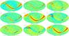 |
Fig. 5 A single column of the Springtide covariance matrix corresponding to a pixel near the ecliptic equator. For description of the normalization, see text. |
Figures 6, 7 show plots of the NCM columns of another reference pixel (number 2047). This pixel is located at the northern ecliptic pole region and it exhibits a very different correlation pattern compared to the previous case. Since the pole is visited frequently through the course of the survey, it becomes correlated with the rest of the map as a whole. Correlation amplitude is increased by a factor of 3 from the equator pixel case (the increase can be seen from the color bar ranges) and there is now a distinct asymmetry between northern and southern hemispheres. As one expects, the asymmetry only appears in optimal and generalized destriping estimates.
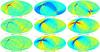 |
Fig. 6 A single column of the MADping covariance matrix corresponding to a pixel at the ecliptic pole. For both ROMA and Madam 1.25s baseline counterparts all visible characteristics remain unchanged. We plot the value of the correlation coefficient, R, multiplied by 103. In order to enhance the features, we have halved the range of the color scale. |
 |
Fig. 7 A single column of the Springtide covariance matrix corresponding to a pixel near the ecliptic north pole. For description of the normalization, see text. |
6.2. Noise covariance validation
In this section we report the results of three different validation tests. We performed a χ2 test, compared the noise biases computed from the matrices and corresponding Monte Carlo maps and finally used the matrices and Monte Carlo maps as inputs to angular power spectrum estimation.
6.2.1. By χ2
Residual noise expected in the recovered maps is Gaussian due to the linear character
of all the mapmaking methods considered here. Thus the noise can be completely described
by its covariance matrix. More specifically, in the absence of any singular modes of the
estimated residual covariance, N, the residual maps,
 , are drawn from a
multivariate Gaussian distribution defined by N.
Therefore, the χ2 statistic, defined as
χ2 = mTN-1m,
is drawn from a χ2 distribution with
3Npix degrees of freedom (d.o.f.).
, are drawn from a
multivariate Gaussian distribution defined by N.
Therefore, the χ2 statistic, defined as
χ2 = mTN-1m,
is drawn from a χ2 distribution with
3Npix degrees of freedom (d.o.f.).
If any singular mode is present we simply replace the matrix, N-1, in the definition of χ2, by a matrix, N′ − 1, which is like N-1 in all respects but has the eigenvalue corresponding to the singular vector set to 0 (see Sect. 3.1). We note that if the eigenvalue decomposition of the matrix N-1 is not available or too costly to compute, we can achieve numerically the same effect by defining N′ = N + η2vvT, where v is a singular vector we want to project out and η2 is a large positive number for which however inversion of N′ is still stable (e.g. Bond et al. 2000). As we subtract one degree of freedom corresponding to the excluded, ill-conditioned eigenmode we expect that there are in total 3Npix − 1 degrees of freedom left in our maps
The χ2 test can be applied, with certain restrictions, to the smoothed maps and matrices. In general, a smoothed matrix will not have any longer the original number of degrees of freedom: some of the small scale eigenmodes have become ill-conditioned (see Sect. 3.3). In this section we regularize the smoothed matrices by omitting the singular eigenmodes.
Singular modes of the original matrix require special attention when smoothing and need
to be treated explicitly if the smoothed version of the ill-conditioned eigenmode,
v, does not belong to the null space of the inverse
smoothed NCM, i.e.,  . To do so, we employ
the same approach as before, replacing the regularized inverse of the smoothed
covariance matrix,
. To do so, we employ
the same approach as before, replacing the regularized inverse of the smoothed
covariance matrix,  ,
by,
,
by, ![Mathematical equation: \begin{eqnarray} &&\tilde{\vec N}^{-1} \rightarrow \left[ \vec {\tilde N} +\eta^2\,\vec L \vec v \left(\vec L \vec v\right)^\mathrm T \right]^{-1} \stackrel{\eta^2 \rightarrow \infty}{\longrightarrow} \vec {\tilde N}^{-1} \nonumber\\&&\qquad \quad- \left( \vec {\tilde N}^{-1}\,\vec L \vec v \right) \left[ \left(\vec L \vec v\right)^t \vec {\tilde N}^{-1} \left(\vec L\vec v\right) \right]^{-1} \left( \vec {\tilde N}^{-1}\,\vec L \vec v \right)^\mathrm T \end{eqnarray}](/articles/aa/full_html/2010/14/aa12606-09/aa12606-09-eq259.png) (47)\arraycolsep1.75ptwhere
L is a smoothing operator, Eq. (26), and the last expression follows from
the Sherman-Morrison-Woodbury formula (Woodbury
1950). This last operation additionally reduces the number of degrees of
freedom by 1 (or whatever number of modes, v is to be
projected out).
(47)\arraycolsep1.75ptwhere
L is a smoothing operator, Eq. (26), and the last expression follows from
the Sherman-Morrison-Woodbury formula (Woodbury
1950). This last operation additionally reduces the number of degrees of
freedom by 1 (or whatever number of modes, v is to be
projected out).
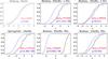 |
Fig. 8 Empirical χ2 distribution functions from the 25
residual noise maps compared with the theoretical cumulative probability density.
The black stair line is the empirical distribution function, the blue solid line
is the theoretical χ2 distribution for
3Npix − 1 = 36863 degrees of freedom. The red dashed
line is the least squares fit of the χ2 distribution
to the experimental distribution (d.o.f. being the fitting parameter). The
horizontal axis is translated to the expected center of the distribution,
⟨ χ2 ⟩ = d.o.f. = 36,863,
and scaled by the expected deviation, |

The Kolmogorov-Smirnov test can be used to test whether a set of samples conforms to
some theoretical distribution. The test estimates the probability of the maximal
difference between the empirical distribution function,  (48)of the observations
xi (in our case the individual
χ2) and the theoretical cumulative distribution function.
Θ(x) is the Heaviside step function. We note that in this work we
take an advantage of the fact that we can simulate the residual noise directly. Though
this is clearly not the case when real data are considered, the tests described here can
be applied to a difference of two sky maps produced by disjoint sets of detectors
operating at the same frequency and can therefore be a useful test of the real life data
processing integrity (e.g. Stompor et al. 2002).
(48)of the observations
xi (in our case the individual
χ2) and the theoretical cumulative distribution function.
Θ(x) is the Heaviside step function. We note that in this work we
take an advantage of the fact that we can simulate the residual noise directly. Though
this is clearly not the case when real data are considered, the tests described here can
be applied to a difference of two sky maps produced by disjoint sets of detectors
operating at the same frequency and can therefore be a useful test of the real life data
processing integrity (e.g. Stompor et al. 2002).
Figure 8 shows the theoretical and Monte Carlo cumulative distribution functions for 25 noise maps in the case of the direct method. Reported p-values are the probabilities of observing this level of disagreement even if the noise description was exact. Conventionally, the level p < 0.05 is considered to be enough to reject the null hypothesis that the distributions match.
In the case of the direct method maps our results show that only optimal (noise) maps and their respective noise covariance are mutually consistent in the light of the χ2 statistics. The good statistical agreement in this case does not depend on the time domain noise characteristics nor map resolution. This is expected given that the noise covariance estimator implemented in the optimal codes, Eq. (18), is an exact expression describing the noise properties in the pixel domain, and that we have assumed perfect knowledge of the time domain noise.
The level of consistency found in the destriping cases varies depending on the underlying time domain properties, i.e., fknee, and on the assumed baseline length. In the case of fknee = 50mHz, we have not found a satisfactory agreement in any of the considered destriping cases. For the lower fknee = 10mHz the results obtained with the generalized destriper, Madam, are satisfactory for the short, 1.25s, baseline choice, and marginal for the long, 60s, choice.
Destriper performance is better using short baselines and at lower knee frequencies. Thus it is evident that failures of the destriping approach to model the residual noise are due to correlated noise that cannot be modeled by baselines of the chosen length. This unmodeled noise is a concern whenever the baseline frequency is lower or comparable to the knee frequency.
But where does the unmodeled noise show? Our three choices of the baseline length
(3600s, 60s and 1.25s) correspond to baseline frequencies 0.28mHz, 17mHz and 800mHz.
These baseline frequencies provide lower limits to the frequencies where unmodeled noise
will manifest. If the lower limit is higher than the satellite spin frequency,
1 / min = 17mHz, it will begin to limit the angular scales at which the unmodeled noise
can manifest. Translated to angular units, the 800mHz threshold is
, multipole ℓ = 24 or size of
a single Nside = 8 pixel. For short baselines or low knee
frequencies the unmodeled noise manifests as a relatively small angular scale
correlation and does not bias the power spectrum estimates at low ℓ.
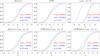 |
Fig. 9 Madam empirical χ2 distribution functions from 60 residual noise maps compared with the theoretical cumulative probability density. For a smoothed map, we count the degrees of freedom as the number of included eigenmodes in the inverse NCM. Top: three sets of low-resolutions maps using just one of the low-resolution methods at a time. The high-resolution maps for INW and smoothing methods had Nside = 1024. Bottom: since it is suboptimal to compute a low-resolution spherical harmonic expansion from a noisy high-resolution map, we test how well the smoothing approach works in conjunction with the two pixel-based downgrading methods. |
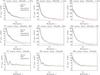 |
Fig. 10 Analytical and mean Monte Carlo noise biases. Gray band is the
1-σ region for the average, computed by dividing the sample
variance by |
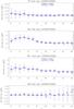 |
Fig. 11 Averaged power spectrum estimates over 25 noise and CMB realizations. The noise has a 10mHz knee frequency. |
We then proceed to study the agreement between downgraded noise maps and the noise covariance matrices. As a test case, we use the Madam NCM for 10mHz knee frequency, 1.25s baselines. We smoothed the covariance matrix using an apodized window function, setting the thresholds to 2Nside and 3Nside respectively. As expected, the smoothed matrix is extremely singular. We compute its inverse by including only the eigenvalues that are greater than 10-2 times the largest eigenvalue, including 20882 of the 36864 available modes.
Figure 9 shows the empirical distribution functions of the χ2. Even though the matrix is computed for the direct method, the inverse noise weighted (INW) maps conform well to it. However, when we apply the smoothing kernel to the high-resolution maps, there is a clear disagreement. This stems from the fact that in this downgrading the high-resolution pixels are not correctly (inverse noise variance) weighted when we compute the low-resolution map. If we first produce a low-resolution direct method or INW map and then smooth it, the agreement is much better. This is shown in the bottom row of Fig. 9.
We conclude that the noise covariance of the low-resolution maps produced by the destriping algorithm needs to be used with care. In the case of low knee frequency, the generalized destriper results are comparable with the optimal results, but we emphasize that, if the accuracy of the noise description in pixel domain is a major concern, then only the optimal techniques are suitable. In the next sections we will reconsider all these low-resolution mapmaking techniques in a context more specific to the large angular scale power spectrum estimation work, which is envisaged as the main application of the low-resolution maps and their covariances.
6.2.2. By noise bias
In this section we describe the calculation of the average angular power spectrum of noise maps, i.e., the noise bias – see Sect. 4.2, using a pseudo Cℓ estimator for which both the NCM estimate and the Monte Carlo map averages are feasible to compute. Testing the noise covariance matrix by comparing estimated and measured noise biases can be viewed as complementary to the χ2 tests described in the previous section. It can certainly provide more information than the plain χ2 test, as instead of simple pass or fail indicator, the noise bias comparison will tell at which angular resolution the noise model agrees with the data. At the same time, the noise bias is less sensitive to the anisotropic features, in this case mainly ring-like structures, present in the residual noise. The noise bias test is more directly relevant for power spectrum estimation.
Figure 10 compares noise bias averages from 25 noise realizations of the maps of the noise residuals to the analytical estimates, Eq. (45), based on the estimated noise covariance matrix. Map spectra are computed using the HEALPix anafast utility and the estimated noise biases using the corresponding map2alm subroutine. We only show the auto-spectra, TT, EE and BB, as the scanning has decoupled the modes to large extent and only minimal coupling between the modes exist.
The error band around the averages is the standard deviation of the individual
Cℓ values divided by
 .
Each plot exhibits up to five curves: direct, inverse noise weighted and harmonic
smoothed noise biases, and two analytical estimates.
.
Each plot exhibits up to five curves: direct, inverse noise weighted and harmonic
smoothed noise biases, and two analytical estimates.
Top row of Fig. 10 displays the noise bias comparison for the high 50mHz knee frequency with short 1.25s Madam baselines. The earlier χ2 plot, Fig. 8, showed a significant disagreement between the maps and the matrix used to derive these biases. In harmonic space the correspondence is significantly better. Since the angular power spectrum does not contain information about the orientation of structures, it may be concluded that the disagreement averages out in the compression.
In contrast with the excellent short baseline results, middle row of Fig. 10 displays an apparent failure of the long Madam 60s baselines to model the high fknee = 50mHz noise. To no surprise, the unmodeled noise above the low 17mHz baseline frequency has passed through the mapmaking process and projected onto the noise maps. As our baseline approximation of the noise is now worse than in Fig. 10, the measured noise bias is higher even though the estimated bias is lower.
Between these two extremes we find the low 10mHz knee frequency cases. For these time lines the level of correlated noise is so low that even extremely long hour baselines do an adequate job estimating the noise bias shown in bottom row of Fig. 10.
At 10mHz the Madam results for long 60s baselines are equivalent with Springtide results: both succeed to estimate noise bias at low knee frequency but should not be used for high knee frequencies as such.
We note that our analytic predictions are well in line with WMAP findings (Hinshaw et al. 2007; Page et al. 2007) and studies of the destriping framework (Efstathiou 2005, 2007).
Our noise bias estimates for EE and BB spectra are equal, but the averaged spectra for the Monte Carlo maps appear visually different in this respect. To ensure that this is only due to Monte Carlo noise we ran Madam in Monte Carlo mode, simulating noise on the fly and avoiding the costs associated with storing of the time-ordered data. After averaging over 117 Nside = 8 noise map spectra we found that the differences between EE and BB noise map spectra were at most 10%.
In the Appendix A.1 we re-plot some of these figures after subtracting the analytical bias and dividing by the Monte Carlo sample deviation to highlight the differences between the analytical and numerical results.
6.2.3. By power spectrum estimation
Our final validation procedure for the noise covariance matrices was to use them in
Cℓ estimation. Due to resource
constraints this exercise was conducted at a lower Nside = 8
resolution. All three mapmaking codes produced maps from the 25 noise realizations. Each
realization was paired with an independent realization of the CMB sky and the co-added
maps were processed using the Bolpol code, an implementation of the QML estimator
described in Sect. 4.1. The 25 power spectrum
estimates for each multipole were then averaged over and the Bolpol-determined error
bars were accordingly divided by .
An example of the results is shown in Fig. 11. These estimates were obtained for the case with the low knee frequency, fknee = 10mHz, using the conventional destriper, Springtide. We note they do not hint unambiguously at any problem with the estimated covariance, even if the χ2 (strongly) and the noise bias (mildly) tests may indicate otherwise. This is likely in part due to a lower sensitivity of the power spectrum test on the one hand and on the other due to the fact that the lower resolution has been used in this last case.
Similar statistically good agreements can also be seen in the case of the higher value of fknee, if the covariance is computed using either the optimal or generalized destriping technique with the short baselines of 1.25 s. If longer baselines are used, i.e., 60 s, the estimates of the polarized spectra, both E and B, are visibly discrepant with the assumed inputs. Similar disagreement can be seen if the off-diagonal elements of the covariance matrices are neglected. In both of these cases, no particular effect on the total intensity spectrum can be noticed in the range of investigated angular scales. We illustrate all these statements in Appendix A.2. These observations emphasize the importance of precise estimation of the noise covariance in particular for the polarized power spectra.
6.3. Low-resolution maps
In the previous sections we have discussed our ability to estimate correctly the properties of the noise present in the low-resolution maps. We have demonstrated that this is indeed the case for all considered resolution downgrading strategies and both optimal and destriper maps. Though in the latter case a baseline length needs to be carefully chosen depending on the time domain noise characteristic.
In this section we focus on the low-resolution maps themselves. We will look at them from three different perspectives, evaluating the level of the mapmaking artifacts left in the maps, the properties of the sky signal and the level of the noise.
In Fig. 12 we show the differences of the noise-free low-resolution maps computed using different downgrading approaches discussed earlier and the input map used for the simulations. The reference low-resolution version of the input map has been obtained via simple binning of the sky signal directly into low-resolution pixels.
In the case of the direct method we see clearly the extra power spread all over the sky in all three Stokes parameters. Any other proposed approach clearly fares much better leading to a substantial decrease of the level of the observed artifacts. This is quantified with the help of the pseudo-spectra in Fig. 13 and in Table 3, where we have collected the root mean square estimates for the signal residual maps.
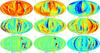 |
Fig. 12 Examples of signal striping. We show the difference between a binned and destriped signal-only maps. Rows correspond to direct Madam results, 1.25s and 60s, and inverse noise weighted 1.25s baseline case respectively. |
Comparison of TT power (rms) in the stripe maps at Nside = 8.
The CMB part of the low-resolution maps also depends on the downgrading technique. These attempt to suppress the high-ℓ (sub pixel) power and therefore can potentially affect the CMB angular power spectrum even within the band of interest. Figure 15 shows the full-sky pseudo-Cℓ spectra averaged over 117 CMB realizations, downgraded using inverse noise weighting and a number of smoothing kernels. In the QML method the situation is slightly more complex, as the quadratic map function is multiplied with the inverse Fisher matrix to produce the QML power spectrum estimate (see Sect. 4.1). The inverse Fisher matrix can correct some of the aliasing effects that cause bias in the power spectra. To simulate the effect of the inverse Fisher in QML we deconvolved our pseudo spectra with a mode coupling kernel that we computed from a map of ones.
Comparison of the spectra shows that it is hard to attain subpercent bias even at ℓ = 2Nside. If these were estimates from an actual power spectrum estimation code with correlated noise and a sky cut, the smoothed covariances would, however, be regularized by adding white noise effectively leading to a considerable uncertainty already at that multipole due to white noise and a sky cut. Methods that produce less than 5% bias for Cℓ estimates at ℓ = 2.5Nside are the Gaussian 10° symmetric beam and the apodized step function for (ℓ1,ℓ2) = (2or2.5Nside,3Nside). The noise weighting and direct low-resolution mapmaking produce similar aliasing effects.
In Fig. 14 we show the actual sky signal spectra estimated for the low-resolution, noiseless maps. It can be seen that the estimated band powers are not drastically affected with respect to the estimates coming from the binned maps. Nevertheless, the case of estimates coming from the direct low-resolution maps show some deviation from the binned case. The bias is most prominent in the BB low multipole estimates. We note that since the signal covariance matrix is ill-conditioned it was regularized by adding a small white NCM (σ ≃ 1μK) and each signal map received a noise realization consistent with this white NCM.
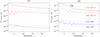 |
Fig. 13 Comparison of CMB and stripe power spectra reveals that the striping can significantly bias the EE and BB power spectrum estimates. Stripe map spectra are computed from maps shown in Fig. 12. |
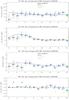 |
Fig. 14 Band power estimates of CMB with CMB and foreground stripes. |
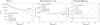 |
Fig. 15 Bandwidth limiting the signal using various window functions. The three panels show the same curves first as raw estimates, then after deconvolving the smoothing and pixel windows and finally after subtracting and dividing by input model. The apodized step window functions (“cosine”) correspond to choices of the thresholds (ℓ1,ℓ2) as (20,24), (16,24) and (16,20) respectively. Here, solid lines are for Gaussian windows and dashed lines for the apodized step functions. |
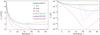 |
Fig. 16 TT noise bias computed from smoothed covariance matrices. Solid lines correspond to the Gaussian window functions and the dashed ones to apodized step functions. Left: linear vertical scale. Right: logarithmic vertical scale. |
None of the proposed downgrading approaches can yield a noise level better than the direct method. This is because noise-weighted downgrading or smoothing both introduce departures from the optimal weighting of the noise present in the data. The expected level of the noise is therefore an important metric with which to compare the different downgraded maps. Figure 16 shows the analytical noise biases evaluated from an Nside = 8 Madam noise covariance matrix after smoothing using the 6 different beam window functions defined in Sect. 5.4 and the unsmoothed case that is a close match to the noise weighted maps. The narrowest Gaussian window function having an FWHM equal to 5°, slightly less than average pixel width, appears pathological due to aliasing effects. The rest of the test cases are more stable but feature a non-negligible amount of aliased power for multipole moments beyond ℓ = 3Nside (the Cℓ are not normalized with the conventional ℓ(ℓ + 1) / 2π).
6.4. Resource requirements
Table 4 lists some CPU time costs for various Nside, baseline length and knee frequency combinations. Being a considerably expensive operation, we have not tested the scaling of the optimal calculation for this particular exercise. See Borrill (1999) for more discussion of scaling. The Madam resource cost scales roughly linearly with respect to the number of pixels and the so-called baseline correlation length.
Resource requirements of the three approaches vary. As with mapmaking, the destriping problem size is related to the chosen baseline offset length. The same consideration applies also for noise covariance estimation. Both the Madam generalized destriper and the MADping covariance calculations scale by the length of the noise filter. ROMA does the calculation in Fourier space and as a results scales as the logarithm of the noise filter length. The MADping algorithm has no dependency (ignoring communication and final file writing) on the number of pixels being used. Although the computation prefactors are not specified, we can see that at Nside = 32, MADping is already more resource efficient than ROMA (cf. rows two and three).
CPU time costs for 1270 GHz detector years = 3 × 10¹⁰ samples.
7. Conclusion
We have presented the formalism and tools to compute the residual noise covariance matrix for three mapmaking paradigms studied for Planck (an optimal method and two destriping methods). The structure of these matrices follows from the scanning strategy but is modulated by the underlying noise model that defines the mapmaking method. The matrices were tested against Monte Carlo noise maps that were processed from correlated noise streams into maps using MADmap, Madam and Springtide mapmaking codes.
The most accurate correspondence between the covariance matrix and the noise maps is, as expected, between the optimal mapmakers, MADmap and ROMA, and their covariance matrices and the two codes produce nearly identical matrices. Both the generalized (Madam) and classical (Springtide) destripers are shown to disregard some medium frequency correlated noise that cannot be modeled by the chosen baseline offset length. It is shown that for a low knee frequency, 10mHz, the Springtide baseline length of 1 h is sufficient to model the correlated noise and compute the residual noise covariance. For a high knee frequency, 50mHz, even the Madam 60s baselines are too long to suffice. However, using a short 1.25s baselines (just 96 samples) the Madam results are extremely close to optimal results even for the high knee frequency.
As a concluding test we used the matrices in actual power spectrum estimation and verified that all methods model residual noise adequately when the noise approximation (baseline length) is short enough to model the correlated noise.
Resource costs of the methods vary greatly. Although both MADping and ROMA arrive at the same result, the implementations differ and the ROMA result scales with the resolution of the map. Both optimal implementations are extremely resource intensive. The Madam method can be used to produce good approximations of the optimal covariance matrices at a fraction of their cost. The covariance matrices for these tests were evaluated for two low resolutions, Nside = 8 and Nside = 32. It is possible to compute the matrices up to Nside = 64 (already 162 gigabytes) or even up to Nside = 128 (2.6TB) but the computational scaling of the methods using the matrices will likely set limits to the usefulness of such resolutions.
We studied two classes of downgrading strategies, those that make an attempt to limit the signal bandwidth and those that do not. The choice of the best downgrading approach depends on both the accuracy of the resulting noise and signal models. First measuring our ability to compute an accurate noise covariance matrix and the second describing our ability to control signal effects such as striping and aliasing.
All methods to produce low-resolution maps have their drawbacks. Direct mapmaking at low resolution produces an unacceptable level of signal striping that is caused by subpixel structure. Downgrading by noise weighting biases the power spectrum through aliasing effects. The frequently used Gaussian beam smoothing has a significant drawback of suppressing the signal at otherwise useful angular resolutions. We find that an apodized step function is able to retain a great deal of signal power up to ℓmax = 2Nside but even then the power spectrum estimates will be biased beyond ℓ = 2.5Nside. However, to accurately evaluate the noise covariance matrix for a smoothed map, we would need to compute an unsmoothed covariance matrix at the high map resolution and then apply the same smoothing kernel to both the matrix and the map. Disregarding this requirement leads to disagreement between the map and the matrix that can be alleviated by combining two or more of the downgrading methods.
We note that, although not considered in this work, most of the complications associated with low resolution mapmaking can be directly addressed by constructing the map in harmonic domain instead of pixel domain (Challinor et al. 2002; Armitage & Wandelt 2004; Armitage-Caplan & Wandelt 2009). A study of residual noise covariance with such methods would make an interesting extension to that presented here.
Of the downgrading methods considered, we consider smoothing, with a suitable choice of the window function and possibly a intermediate downgrading step by inverse noise weighting, to produce the best possible low-resolution maps for power spectrum analysis.
We presented in this work a method to compute the residual noise covariance of a smoothed, bandwidth-limited map. The method was shown to produce an accurate description of the noise in the smoothed maps when both the map and the matrix agree prior to smoothing. Our method of smoothing the covariance matrix makes it possible to consider bandwidth limited low-resolution maps and produce subpercent level unbiased power spectrum estimates up to ℓ = 2.5Nside.
In this work we have assumed a single frequency channel, uncorrelated noise between detectors, noise that is white at high frequencies and full sky coverage. In further work any of these constraints can be lifted. The only application that we used the covariance matrix was in power spectrum estimation. The downgrading methods that suit power spectrum analyses best may not be optimal for different low-resolution analysis, e.g., study of large scale topology. A relevant future direction to explore is the use of the covariance matrices as inputs in a likelihood code for cosmological parameters.
HEALPix resolution is reported as either Nside
or r, related by
Nside = 2r. A HEALPix map
contains  pixels.
Side and Main refer to two detector branches downstream from the orthomode transducer that separates the two orthogonal linear polarizations.
 ,
where σ and fsample were defined in
Eq. (19). The 70GHz detectors had
fsample = 76.8Hz.
,
where σ and fsample were defined in
Eq. (19). The 70GHz detectors had
fsample = 76.8Hz.
A double precision (64 bit) matrix is numerically ill-conditioned when the condition number exceeds approximately 1012 (Press 1992). For our matrices the situation is not as dire but the first eigenmode still deserves special attention.
In a HEALPix map the Stokes parameters Q and U at a point in the sky are defined in a (x, y, z) reference coordinate, where the x-axis is along the meridian and points to south, the y-axis is along the latitude and points to east, and the z-axis points to the sky (Górski et al. 2005).
Actually, the global offset mode is only nearly singular. This is due to our assumed noise power spectrum, which is finite at zero frequency. In a more realistic case the offsets of the stationary segments will be however unknown, corresponding to an infinite amplitude at zero frequency. The noise covariance in such cases should be therefore considered to be strictly singular with the global offset being the singular eigenvector. In such cases the noise weighting on the right term of the map making equation, Eq. (17), will force the offset of each of the stationary data segments to be strictly zero. This may not be a sufficiently good approximation in particular for short stationary time segments. This could, however, be alleviated by introducing the segment offsets as extra degrees of freedom contained in the vector, x, (e.g. Stompor et al. 2002).
Acknowledgments
The work reported in this paper was done by the CTP Working Group of the Planck Consortia. Planck is a mission of the European Space Agency. We acknowledge the use of the CAMB (http://camb.info) code for generating theoretical CMB spectra. Some of the results in this paper have been derived using the HEALPix package (Górski et al. 2005). We acknowledge the use of version 1.6.3 of the Planck sky model, prepared by the members of Planck Working Group 2. This work has made use of the Planck satellite simulation package (Level-S), which is assembled by the Max Planck Institute for Astrophysics Planck Analysis Centre (MPAC). This research used resources of the National Energy Research Scientific Computing Center, which is supported by the Office of Science of the U.S. Department of Energy under Contract No. DE-AC02-05CH11231. We thank CSC (Finland) for computational resources. RK wishes to thank the Jenny and Antti Wihuri Foundation and the Väisälä Foundation for financial support. This work was supported by the Academy of Finland grants 121703 and 121962. HKS thanks Waldemar von Frenckells stiftelse and Magnus Ehrnrooth Foundation for financial support. We acknowledge support from ASI, contract Planck LFI Activity of Phase E2. RS acknowledges partial support of the European Commission Marie Curie IR Grant, MIRG-CT-2006-036614.
References
- Armitage, C., & Wandelt, B. D. 2004, Phys. Rev. D, 70, 123007 [NASA ADS] [CrossRef] [Google Scholar]
- Armitage-Caplan, C., & Wandelt, B. D. 2009, ApJS, 181, 533 [NASA ADS] [CrossRef] [Google Scholar]
- Ashdown, M. A. J., Baccigalupi, C., Balbi, A., et al. 2007a, A&A, 471, 361 [NASA ADS] [CrossRef] [EDP Sciences] [Google Scholar]
- Ashdown, M. A. J., Baccigalupi, C., Balbi, A., et al. 2007b, A&A, 467, 761 [NASA ADS] [CrossRef] [EDP Sciences] [Google Scholar]
- Ashdown, M. A. J., Baccigalupi, C., Bartlett, J. G., et al. 2009, A&A, 493, 753 [NASA ADS] [CrossRef] [EDP Sciences] [Google Scholar]
- Benabed, K., Cardoso, J. F., Prunet, S., & Hivon, E. 2009, MNRAS, 400, 219 [NASA ADS] [CrossRef] [Google Scholar]
- Bond, J. R., Jaffe, A. H., & Knox, L. 1998, Phys. Rev. D, 57, 2117 [NASA ADS] [CrossRef] [Google Scholar]
- Bond, J. R., Jaffe, A. H., & Knox, L. E. 2000, ApJ, 533, 19 [NASA ADS] [CrossRef] [Google Scholar]
- Borrill, J. 1999, in Proceedings of the 5th European SGI/Cray MPP Workshop, Bologna, Italy [Google Scholar]
- Cantalupo, C. M., Borrill, J. D., Jaffe, A. H., Kisner, T. S., & Stompor, R. 2010, ApJS, 187, 212 [NASA ADS] [CrossRef] [Google Scholar]
- Challinor, A., Fosalba, P., Mortlock, D., et al. 2000, Phys. Rev. D, 62, 123002 [NASA ADS] [CrossRef] [Google Scholar]
- Challinor, A. D., Mortlock, D. J., van Leeuwen, F., et al. 2002, MNRAS, 331, 994 [NASA ADS] [CrossRef] [Google Scholar]
- de Bernardis, P., Ade, P. A. R., Bock, J. J., et al. 2000, Nature, 404, 955 [NASA ADS] [CrossRef] [PubMed] [Google Scholar]
- de Gasperis, G., Balbi, A., Cabella, P., Natoli, P., & Vittorio, N. 2005, A&A, 436, 1159 [NASA ADS] [CrossRef] [EDP Sciences] [Google Scholar]
- Delabrouille, J. 1998, A&AS, 127, 555 [Google Scholar]
- Dupac, X., & Tauber, J. 2005, A&A, 430, 363 [NASA ADS] [CrossRef] [EDP Sciences] [Google Scholar]
- Efstathiou, G. 2005, MNRAS, 356, 1549 [NASA ADS] [CrossRef] [Google Scholar]
- Efstathiou, G. 2007, MNRAS, 380, 1621 [NASA ADS] [CrossRef] [Google Scholar]
- Efstathiou, G., Gratton, S., & Paci, F. 2009, MNRAS, 397, 1355 [NASA ADS] [CrossRef] [Google Scholar]
- Górski, K. M., Banday, A. J., Bennett, C. L., et al. 1996, ApJ, 464, L11 [NASA ADS] [CrossRef] [Google Scholar]
- Górski, K. M., Hivon, E., Banday, A. J., et al. 2005, ApJ, 622, 759 [NASA ADS] [CrossRef] [Google Scholar]
- Gruppuso, A., de Rosa, A., Cabella, P., et al. 2009, MNRAS, 400, 463 [NASA ADS] [CrossRef] [Google Scholar]
- Hanany, S., Ade, P., Balbi, A., et al. 2000, ApJ, 545, L5 [NASA ADS] [CrossRef] [Google Scholar]
- Hinshaw, G., Nolta, M. R., Bennett, C. L., et al. 2007, ApJS, 170, 288 [NASA ADS] [CrossRef] [Google Scholar]
- Jarosik, N., Barnes, C., Bennett, C. L., et al. 2003, ApJS, 148, 29 [NASA ADS] [CrossRef] [Google Scholar]
- Jarosik, N., Barnes, C., Greason, M. R., et al. 2007, ApJS, 170, 263 [NASA ADS] [CrossRef] [Google Scholar]
- Keihänen, E., Kurki-Suonio, H., Poutanen, T., Maino, D., & Burigana, C. 2004, A&A, 428, 287 [NASA ADS] [CrossRef] [EDP Sciences] [Google Scholar]
- Keihänen, E., Kurki-Suonio, H., & Poutanen, T. 2005, MNRAS, 360, 390 [NASA ADS] [CrossRef] [Google Scholar]
- Keihänen, E., Keskitalo, R., Kurki-Suonio, H., Poutanen, T., & Sirviö, A.-S. 2010, A&A, 510, A57 [NASA ADS] [CrossRef] [EDP Sciences] [Google Scholar]
- Kuo, C. L., Ade, P. A. R., Bock, J. J., et al. 2004, ApJ, 600, 32 [NASA ADS] [CrossRef] [Google Scholar]
- Kurki-Suonio, H., Keihänen, E., Keskitalo, R., et al. 2009, A&A, 506, 1511 [NASA ADS] [CrossRef] [EDP Sciences] [Google Scholar]
- Maino, D., Burigana, C., Górski, K. M., Mandolesi, N., & Bersanelli, M. 2002, A&A, 387, 356 [NASA ADS] [CrossRef] [EDP Sciences] [Google Scholar]
- Masi, S., Ade, P. A. R., Bock, J. J., et al. 2006, A&A, 458, 687 [NASA ADS] [CrossRef] [EDP Sciences] [Google Scholar]
- Natoli, P., de Gasperis, G., Gheller, C., & Vittorio, N. 2001, A&A, 372, 346 [NASA ADS] [CrossRef] [EDP Sciences] [Google Scholar]
- Natoli, P., Marinucci, D., Cabella, P., de Gasperis, G., & Vittorio, N. 2002, A&A, 383, 1100 [NASA ADS] [CrossRef] [EDP Sciences] [Google Scholar]
- Page, L., Hinshaw, G., Komatsu, E., et al. 2007, ApJS, 170, 335 [NASA ADS] [CrossRef] [Google Scholar]
- Planck Collaboration 2005, ESA-SCI, 1, preprint [arXiv:astro-ph/0604069] [Google Scholar]
- Poutanen, T., de Gasperis, G., Hivon, E., et al. 2006, A&A, 449, 1311 [NASA ADS] [CrossRef] [EDP Sciences] [Google Scholar]
- Press, W. H. 1992, Numerical Recipes in FORTRAN: The Art of Scientific Computing, 2nd ed. (Cambridge University Press) [Google Scholar]
- Stompor, R., & White, M. 2004, A&A, 419, 783 [NASA ADS] [CrossRef] [EDP Sciences] [Google Scholar]
- Stompor, R., Balbi, A., Borrill, J., et al. 2002, Phys. Rev. D, 65, 022003 [Google Scholar]
- Tegmark, M. 1997, Phys. Rev. D, 55, 5895 [Google Scholar]
- Tegmark, M., & de Oliveira-Costa, A. 2001, Phys. Rev. D, 64, 063001 [NASA ADS] [CrossRef] [Google Scholar]
- Woodbury, M. A. 1950, Statistical Research Group, Memo. Rep., 42, 4 [Google Scholar]
- Wright, E. L., Bennett, C. L., Górski, K. M., Hinshaw, G., & Smoot, G. F. 1996, ApJ, 464, L21 [NASA ADS] [CrossRef] [Google Scholar]
Appendix A: Additional material
A.1. Noise biases
For completeness, we present in Fig. A.1 the noise bias computed from the MADmap NCM and the 25 corresponding noise maps and the Madam bias for fknee = 10 mHz and 60 s baseline.
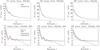 |
Fig. A.1 Analytical and mean Monte Carlo noise biases. Gray band is the 1-σ
region for the average, computed by dividing the sample variance
by |
 |
Fig. A.2 Averaged noise biases after subtracting the analytical estimate and normalizing with the standard deviation. This plot contains the same curves as Fig. A.1. |
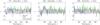 |
Fig. A.3 Averaged noise biases after subtracting the analytical estimate and normalizing with the standard deviation. This plot contains the same curves as the top row of Fig. 10. |
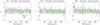 |
Fig. A.4 Averaged noise biases after subtracting the analytical estimate and normalizing with the standard deviation. This plot contains the same curves as the bottom row of Fig. 10. |
To highlight differences between the estimates and simulated noise maps we also show the fractional differences in Figs. A.2–A.4. These plots complete the ones presented in Sect. 6.2.2.
A.2. Power spectra
Here we present another successful test of the covariance matrix used in power spectrum estimation, Fig. A.5. We also show how the power spectrum estimates can be used to pick out inaccurate residual noise covariances in Fig. A.6.
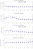 |
Fig. A.5 Averaged power spectrum estimates over 25 noise and CMB realizations. The noise has a 50mHz knee frequency. |
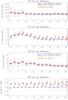 |
Fig. A.6 Averaged power spectrum estimates over 25 noise and CMB realizations. The noise has a 50mHz knee frequency. |
A.3. Singularities
As we have pointed out in Sect. 3.1, the inversion of the inverse noise covariance matrix, N-1, Eqs. (18) and (9), often needs to be regularized due to the presence of singular or numerically singular modes. In this section we discuss the origin of such modes.
We first note that in all cases considered here the inverse covariance can be expressed
as 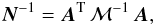 (A.1)where
ℳ-1 is defined to be,
(A.1)where
ℳ-1 is defined to be,
 (A.2)}We
assume that the pointing matrix, A, has full column rank,
and thus
Ax = 0 ⇒ x = 0.
This is equivalent to an assumption that the sky signal can indeed be estimated from a
given data set. Though this may not be always the case, in particular for the polarization
sensitive experiments, it can usually be achieved if some of the ill-constrained pixels
are removed from consideration. Given this assumption, the problem of the singular modes
of N-1 becomes that of the matrix,
ℳ-1, defined above.
(A.2)}We
assume that the pointing matrix, A, has full column rank,
and thus
Ax = 0 ⇒ x = 0.
This is equivalent to an assumption that the sky signal can indeed be estimated from a
given data set. Though this may not be always the case, in particular for the polarization
sensitive experiments, it can usually be achieved if some of the ill-constrained pixels
are removed from consideration. Given this assumption, the problem of the singular modes
of N-1 becomes that of the matrix,
ℳ-1, defined above.
Let us consider the optimal map case first. The matrix ℳ-1 is equal to the inverse of the time-domain noise covariance, 𝒩-1. The latter, Sect. 2.2, is a block Toeplitz matrix with each block defined by an inverse of the noise power spectrum, Eq. (19). Each of those blocks describes the noise properties of one of the stationary data segments assumed in the simulations. For each block the eigenmodes corresponding to the lowest frequencies as permitted by the length of the segment have eigenvalues vastly smaller than the high frequency modes. These modes can therefore lead to near singularities. This is specifically true for zero-frequency modes corresponding to an offset of each of the stationary data segments. The (near) null space of the full matrix will be therefore spanned by all such vectors corresponding to each of the segments.
Due to projection effects, not all of those modes result in singular modes of the final pixel domain noise covariance. However, if for a mode, t, from the null space of 𝒩-1, there exists a pixel domain vector, x, such as t = Ax, the inverse noise covariance will be singular with eigenvector equal to x.
In the studied case, the scanning strategy is such that the sky areas observed in each of the stationary periods overlap, which efficiently removes most of the potential degenerate vectors. In fact only a single pixel-domain IQU vector of which the I part is one and all the others zero, called hereafter a global offset, can potentially be singular. We will indeed confirm these expectations via numerical results later10.
In the case of the maps produced with the destriper codes in the absence of any priors, i.e., 𝒫-1 = 0 the ℳ-1 matrix has as many singular vectors as the baseline offsets defined by the columns of the offset “pointing” matrix, B. However, as long as all of the offsets cross on the sky the only singular vector of the pixel-domain covariance will again correspond to the global offset vector as in the optimal map case. We note however that unlike in that case, this time this vector is exactly singular. If a prior is employed, as is the case in both the classical and generalized implementations of the destriper technique discussed here, the columns of the matrix B are no longer singular vectors of the matrix ℳ-1, nor is the global offset vector a singular vector of N. Nevertheless, at least for some common choices of the prior the global offset vector remains nearly singular.
All Tables
All Figures
|
Fig. 1 Noise model (dashed lines) and the spectra of simulated noise (solid lines). The two sets of curves correspond to the two considered knee frequencies with fmin = 1.15 × 10⁻⁵ and α = 1.7. |
| In the text | |
|
Fig. 2 Eigenspectra of the inverse covariance matrices N-1. MADping, ROMA and Madam results for fknee = 50mHz overlap completely. Springtide results are for 10mHz. |
| In the text | |
|
Fig. 3 Top: MADping pixel variances for temperature and polarization and the reciprocal condition number of the pixel observation matrices. Bottom: correlation coefficient × 103 between I − Q, I − U and Q − U pixels. This part of the noise covariance is dominated by white noise which is modeled equivalently in all three paradigms. Hence, MADmap, ROMA, Madam and Springtide results are nearly identical. Maps are rotated into galactic coordinates to show the structure near the ecliptic poles. |
| In the text | |
|
Fig. 4 A single column of the MADping covariance matrix corresponding to a pixel at the ecliptic equator. For both ROMA and Madam 1.25s baseline counterparts all visible characteristics remain unchanged. We plot the value of the correlation coefficient, R, multiplied by 103. In order to enhance the features, we have halved the range of the color scale. |
| In the text | |
|
Fig. 5 A single column of the Springtide covariance matrix corresponding to a pixel near the ecliptic equator. For description of the normalization, see text. |
| In the text | |
|
Fig. 6 A single column of the MADping covariance matrix corresponding to a pixel at the ecliptic pole. For both ROMA and Madam 1.25s baseline counterparts all visible characteristics remain unchanged. We plot the value of the correlation coefficient, R, multiplied by 103. In order to enhance the features, we have halved the range of the color scale. |
| In the text | |
|
Fig. 7 A single column of the Springtide covariance matrix corresponding to a pixel near the ecliptic north pole. For description of the normalization, see text. |
| In the text | |
|
Fig. 8 Empirical χ2 distribution functions from the 25
residual noise maps compared with the theoretical cumulative probability density.
The black stair line is the empirical distribution function, the blue solid line
is the theoretical χ2 distribution for
3Npix − 1 = 36863 degrees of freedom. The red dashed
line is the least squares fit of the χ2 distribution
to the experimental distribution (d.o.f. being the fitting parameter). The
horizontal axis is translated to the expected center of the distribution,
⟨ χ2 ⟩ = d.o.f. = 36,863,
and scaled by the expected deviation, |
| In the text | |
|
Fig. 9 Madam empirical χ2 distribution functions from 60 residual noise maps compared with the theoretical cumulative probability density. For a smoothed map, we count the degrees of freedom as the number of included eigenmodes in the inverse NCM. Top: three sets of low-resolutions maps using just one of the low-resolution methods at a time. The high-resolution maps for INW and smoothing methods had Nside = 1024. Bottom: since it is suboptimal to compute a low-resolution spherical harmonic expansion from a noisy high-resolution map, we test how well the smoothing approach works in conjunction with the two pixel-based downgrading methods. |
| In the text | |
|
Fig. 10 Analytical and mean Monte Carlo noise biases. Gray band is the
1-σ region for the average, computed by dividing the sample
variance by |
| In the text | |
|
Fig. 11 Averaged power spectrum estimates over 25 noise and CMB realizations. The noise has a 10mHz knee frequency. |
| In the text | |
|
Fig. 12 Examples of signal striping. We show the difference between a binned and destriped signal-only maps. Rows correspond to direct Madam results, 1.25s and 60s, and inverse noise weighted 1.25s baseline case respectively. |
| In the text | |
|
Fig. 13 Comparison of CMB and stripe power spectra reveals that the striping can significantly bias the EE and BB power spectrum estimates. Stripe map spectra are computed from maps shown in Fig. 12. |
| In the text | |
|
Fig. 14 Band power estimates of CMB with CMB and foreground stripes. |
| In the text | |
|
Fig. 15 Bandwidth limiting the signal using various window functions. The three panels show the same curves first as raw estimates, then after deconvolving the smoothing and pixel windows and finally after subtracting and dividing by input model. The apodized step window functions (“cosine”) correspond to choices of the thresholds (ℓ1,ℓ2) as (20,24), (16,24) and (16,20) respectively. Here, solid lines are for Gaussian windows and dashed lines for the apodized step functions. |
| In the text | |
|
Fig. 16 TT noise bias computed from smoothed covariance matrices. Solid lines correspond to the Gaussian window functions and the dashed ones to apodized step functions. Left: linear vertical scale. Right: logarithmic vertical scale. |
| In the text | |
|
Fig. A.1 Analytical and mean Monte Carlo noise biases. Gray band is the 1-σ
region for the average, computed by dividing the sample variance
by |
| In the text | |
|
Fig. A.2 Averaged noise biases after subtracting the analytical estimate and normalizing with the standard deviation. This plot contains the same curves as Fig. A.1. |
| In the text | |
|
Fig. A.3 Averaged noise biases after subtracting the analytical estimate and normalizing with the standard deviation. This plot contains the same curves as the top row of Fig. 10. |
| In the text | |
|
Fig. A.4 Averaged noise biases after subtracting the analytical estimate and normalizing with the standard deviation. This plot contains the same curves as the bottom row of Fig. 10. |
| In the text | |
|
Fig. A.5 Averaged power spectrum estimates over 25 noise and CMB realizations. The noise has a 50mHz knee frequency. |
| In the text | |
|
Fig. A.6 Averaged power spectrum estimates over 25 noise and CMB realizations. The noise has a 50mHz knee frequency. |
| In the text | |
Current usage metrics show cumulative count of Article Views (full-text article views including HTML views, PDF and ePub downloads, according to the available data) and Abstracts Views on Vision4Press platform.
Data correspond to usage on the plateform after 2015. The current usage metrics is available 48-96 hours after online publication and is updated daily on week days.
Initial download of the metrics may take a while.