| Issue |
A&A
Volume 699, July 2025
|
|
|---|---|---|
| Article Number | A375 | |
| Number of page(s) | 21 | |
| Section | Extragalactic astronomy | |
| DOI | https://doi.org/10.1051/0004-6361/202554682 | |
| Published online | 25 July 2025 | |
X-ray investigation of the remarkable galaxy group Nest200047
1
Astronomical Institute ‘Anton Pannekoek’, University of Amsterdam, Science Park 904, 1098 XH Amsterdam, The Netherlands
2
SRON, Netherlands Institute for Space Research, Niels Bohrweg 4, 2333 CA Leiden, The Netherlands
3
Leiden Observatory, Leiden University, PO Box 9513, 2300 RA Leiden, The Netherlands
4
Kavli Institute for the Physics and Mathematics of the Universe, The University of Tokyo, Kashiwa, Chiba 277-8583, Japan
5
Department of Theoretical Physics and Astrophysics, Faculty of Science, Masaryk University, Kotlářská 2, 602 00 Brno, Czech Republic
6
Istituto Nazionale di Astrofisica (INAF) – Istituto di Radioastronomia (IRA), via P. Gobetti 101, 40129 Bologna, Italy
7
Max Planck Institute for Astrophysics, Karl-Schwarzschild-Str. 1, D-85741 Garching, Germany
8
Space Research Institute (IKI), Profsoyuznaya 84/32, Moscow 117997, Russia
9
Universitäts-Sternwarte, Fakultät für Physik, Ludwig-Maximilians-Universität München, Scheinerstr.1, 81679 München, Germany
10
INAF/IASF-Milano, Via A. Corti 12, I-20133 Milano, Italy
11
University of Hamburg, Hamburger Sternwarte, Gojenbergsweg 112, 21029 Hamburg, Germany
12
Astro Space Center of P.N. Lebedev Physical Institute of the RAS, Profsoyuznaja 84/32, 117997 Moscow, Russia
13
Center for Astrophysics | Harvard & Smithsonian, 60 Garden Street, Cambridge, MA 02138, USA
⋆ Corresponding authors: a.majumder@sron.nl, a.simionescu@sron.nl
Received:
21
March
2025
Accepted:
12
June
2025
Context. Galaxy groups are more susceptible to feedback from the central active galactic nuclei (AGNs) due to their lower gravitational binding energy compared to clusters. This makes them ideal laboratories to study feedback effects on the overall energy and baryonic mass budget.
Aims. We study the LOFAR-detected galaxy group Nest200047, where there is clear evidence of multiple generations of radio lobes from the AGN. Using 140 ks Chandra and 25 ks XMM-Newton data, we investigated thermodynamic properties of the intragroup medium, including any excess energy due to the central AGN. We also investigated the X-ray properties of the central black hole and constrained the 2−10 keV X-ray flux.
Methods. We used spectral analysis techniques to measure various thermodynamic profiles across the whole field of view. We also used both imaging and spectral analysis to detect and estimated the energy deposited by potential shocks and cavities. Due to the faint emission from the object beyond the core, various background effects were considered.
Results. Nest200047 has significant excess entropy, and the AGN likely contributes to a part of it. There is an excess energy of (5−6.5)×1060 erg within 400 kpc, exceeding the binding energy. The pressure profile indicates that gas is likely being ejected from the system, resulting in a baryon fraction of ∼4% inside r500. From scaling relations, we estimated a black hole mass of (1−4)×109 M⊙. An upper limit of 2.1×1040 erg s−1 was derived on the black hole bolometric luminosity, which is ∼2.5% of the Bondi accretion power.
Conclusions. Nest200047 is likely part of a class of over-heated galaxy groups, such as ESO 3060170, AWM 4, and AWM 5. Such excessive heating may lead to high quenching of star formation. Moreover, the faint X-ray nuclear emission in Nest is likely due to the accretion energy being converted into jets rather than radiation.
Key words: shock waves / methods: data analysis / galaxies: active / galaxies: groups: individual: Nest200047
© The Authors 2025
 Open Access article, published by EDP Sciences, under the terms of the Creative Commons Attribution License (https://creativecommons.org/licenses/by/4.0), which permits unrestricted use, distribution, and reproduction in any medium, provided the original work is properly cited.
This article is published in open access under the Subscribe to Open model. Subscribe to A&A to support open access publication.
1. Introduction
Radio-mode feedback from active galactic nuclei (AGNs) plays a key role in regulating the cooling and star formation in a broad range of halo masses (Churazov et al. 2000; Bîrzan et al. 2004; Best et al. 2006; Werner et al. 2019). The jets from the central AGN often create observable structures, such as shocks, that transfer energy to the ambient medium and X-ray cavities by expelling gas from the core (e.g., Begelman & Cioffi 1989; McNamara et al. 2001; Fabian et al. 2006; Wise et al. 2007; Simionescu et al. 2009). Although our understanding of such mechanisms has improved over the years (for reviews, see McNamara & Nulsen 2007; Simionescu et al. 2019), the effect of multiple generations of AGN outbursts on the ambient medium remains an interesting problem. Multi-generational outbursts are expected from numerical simulations (e.g., Rosas-Guevara et al. 2016; DeGraf & Sijacki 2017), and their signatures have been observed in the radio band as multiple pairs of radio lobes interacting with the ambient medium (see Morganti 2017, 2024 for reviews). Such evidence of recurrent outbursts has also been seen in X-rays. Although more recent outbursts are often associated with cavities, the older outbursts have different evolutionary paths that sometimes create X-ray bright arms of low-entropy gas (M87; Forman et al. 2007; Werner et al. 2010) or density and temperature ripples (Cygnus A; Majumder et al. 2024). Extending such studies to a larger number of multiple-outburst systems is important for further pinpointing the details of AGN feedback evolution.
While known examples of multiple generations of outbursts are mostly limited to clusters (e.g., Vantyghem et al. 2014; Biava et al. 2021), the famous example of NGC 5813 and NGC 5044 (Randall et al. 2011; Schellenberger et al. 2021) shows that such an evolutionary history is possible for galaxy groups as well. Galaxy groups lie in a critical mass regime (1013−1014 M⊙), where the hot gas is still sufficiently bright to be observable in X-rays but where AGN feedback may more closely resemble the mechanism needed to quench star formation in individual galaxy haloes. In particular, the energy supplied by the central AGN can exceed the gravitational binding energy of halo gas particles, which is not the case in more massive galaxy clusters (Eckert et al. 2021; Ayromlou et al. 2023). Therefore, further exploring the impact of multi-generation AGN feedback on the intragroup medium (IGrM) can lead to a better understanding of their impact on the evolutionary history of massive galaxies.
The Low-Frequency Array (LOFAR) Two-Meter Sky Survey (LoTSS; Shimwell et al. 2019) and the extended ROentgen Survey with an Imaging Telescope Array (eROSITA) X-ray telescope (Predehl et al. 2021) on board the Spektrum Roentgen Gamma (SRG) orbital observatory (Sunyaev et al. 2021) have recently revealed a truly spectacular example of recurring AGN feedback in a largely unexplored, nearby (z = 0.01795±0.00015; Huchra et al. 2012) galaxy group called Nest200047 (2MASS survey; Tully 2015). The radio and X-ray properties of the object from those investigations were first reported by Brienza et al. (2021). In the radio band, two freshly injected radio lobes, each roughly extending 30 arcsec (11 kpc in projection) in length from the group center, are being inflated by the central AGN associated with the brightest group galaxy, MCG+05-10-007 (A lobes in Figure 1). Farther away, two more radio bubbles (B1 and B2) extend out to radii of 100 arcsec (37 kpc) from the optical centroid of the host galaxy. A third pair of radio lobes (C1 and C2) can be seen between 100−275 arcsec (37−100 kpc) from the AGN, while farther still, the lobes D1 and D3 extend out to a 10 arcmin radius (220 kpc), rivaling the large radio structures found in more massive galaxy clusters (Lane et al. 2004; McNamara et al. 2005; Wise et al. 2007). The outermost lobes exhibit a striking array of complex filamentary radio structures (D2), likely preserved by magnetic fields, showing sharp bends and double strands of very narrow emission. They may represent a rare case of an AGN bubble in its very late stages of evolution, as it is being deformed and shredded by instabilities and possibly in the process of being mixed with the IGrM on small scales. No other radio galaxy in the current LoTSS database shares a similar morphology. The shallow (645 s) eROSITA scan of the object (Brienza et al. 2021), on the other hand, revealed edge-brightening around the radio bubbles that were classified as cavities with powers upwards of 1042 erg s−1. The object has a temperature of ∼2 keV within 13 arcmin and a 0.5−2.0 keV luminosity of (5−10)×1042 erg s−1 within 30 arcmin. More recently, Brienza et al. (2025) performed a more detailed spectral analysis over a broad radio band (53–1518 MHz) using the upgraded Giant Metrewave Radio Telescope (uGMRT; Gupta et al. 2017), MeerKAT (Jonas & MeerKAT Team 2016), and the Karl G. Jansky Very Large Array (VLA; Perley et al. 2011). This recent work estimated the duration of the jet activity for different bubbles to be between 50–100 Myr.
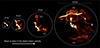 |
Fig. 1. LOFAR image of the galaxy group Nest200047, focusing on various spatial scales to highlight the four consecutive AGN outbursts detected in this system (Brienza et al. 2021). |
In this study, we report the results of the first pointed X-ray observations performed for this galaxy group. We present the X-ray morphology and thermodynamic profiles of the object and estimate energy injection by the radio lobes using Chandra and XMM-Newton data. The high spatial resolution of Chandra allows us to probe any deviation from the expected smooth thermodynamic profiles under hydrostatic equilibrium, while XMM's sensitivity at low energy allows us to probe the outskirts more effectively. Since the object is nearby, Chandra's spatial resolution also allows us to put constraints on the black hole mass and X-ray properties of the central AGN.
We begin in Sect. 2 by presenting the observations and the data reduction methods applied in this work. In Sect. 3, we describe the large-scale features in the X-ray data and highlight any hints of AGN feedback. A detailed description of the spectral analysis method is discussed in Sect. 4, with more details in Sects. C and D. All thermodynamic profiles are then shown and discussed in Sect. 5. Possible deviations from smooth density profiles are discussed in Sect. 6 and then followed by an estimation of the energetics of a tentatively detected cavity in Sect. 7. The mass estimate and X-ray properties of the central supermassive black hole follow in Sect. 8. We conclude with a summary and conclusion of our results in Sect. 9.
A ΛCDM cosmology has been assumed in this work with H0 = 70 km s−1 Mpc−1, ΩΛ = 0.7, and Ωm = 0.3. The corresponding linear scale at the redshift of Nest200047 is 21.9 kpc per arcmin. All errors reported are of 1σ significance.
2. Observations and data reduction
2.1. XMM-Newton
Nest200047 (hereafter Nest) was observed by XMM-Newton on 13-09-2021 for a total exposure of 46 ks. We analyzed the exposure (ObsID: 0883620101) with Science Analysis Software (SAS) v21.0.0 and the latest calibration files. The observation was heavily affected by soft proton flares. We reprocessed the MOS and PN event files from the Observation Data Files (ODF) with SAS tools emproc and epproc, respectively. Furthermore, we created a separate out-of-time (OoT) event file for the PN observation with epproc. The MOS event files were then checked for anomalous soft X-ray noise (Kuntz & Snowden 2008; Stuhlinger 2008) with the SAS tool emanom. The tool flagged CCD 4 of MOS1 as “bad” and CCD 5 of MOS2 as “intermediate”. The MOS1 CCD 4 was henceforth removed from all subsequent analysis, while CCD 5 of MOS2 was kept after checking the spectrum from part of this chip visually. Despite this cleaning, we still found anomalous soft X-ray noise below 1 keV in MOS1 spectra from the central CCD upon visual inspection. We, therefore, discarded the MOS1 spectrum from the central CCD below 1 keV for spectral analysis (see Sect. A for more discussion).
To reduce the heavy soft proton contamination, we filtered all event files as follows: The MOS events were binned in the energy range of 10−12 keV in 100 s intervals. We did the same with the PN events but in the energy range of 10−14 keV. We then fitted each count rate histogram with a Gaussian function to determine the mean (μ) and the standard deviation (σ). All events with a count rate greater than 1σ from the mean were removed from all subsequent analysis. We then focused on removing extremely fast flares by binning the events in the aforementioned energy ranges in 20 s intervals and repeated the Gaussian fits. All events with a count rate greater than 2σ from the mean were removed from all subsequent analysis as well. We report the clean exposure times from each instrument in Table 1. For PN, we applied the same Good Time Intervals (GTIs) to the OoT event file as to the normal observation.
Chandra and XMM-Newton observation log.
For suitable MOS particle background event lists, we used the integrated filter wheel closed (FWC) data1 (Rev. 230 – Rev. 4027). Since there is no suitable out of field of view (FOV) region for PN (Zhang et al. 2020; Marelli et al. 2021), we chose a PN FWC observation (Event list: 3927_0810811601_EPN_S017) that was performed soon before the Nest observation. The FWC files of each instrument were then reprojected onto the same sky coordinates as the Nest observation using the SAS task evproject.
All FOV events in both the observation and the FWC files were screened with the conditions PATTERN< = 12 and (FLAG & 0x766ba000) == 0 for MOS, while the condition PATTERN< = 4 and FLAG= = 0 was chosen for PN. Separate out of FOV event files were also created with the condition #XMMEA_16 for imaging analysis. This flag screens bad event grades but keeps valid out of field of view events.
2.2. Chandra
The galaxy group Nest has been observed for a total of ∼150 ks with Chandra from 21-11-2022 to 18-12-2022. We reprocessed and analyzed all observations in the Chandra data archive using CIAO 4.15 (Fruscione et al. 2006) and CALDB 4.10.7. We used the CIAO tool chandra_repro to create level 2 event files along with the condition check_vf_pha = yes for additional cleaning of particle background in VFAINT mode observations. All reprocessed event files were checked for flares using the same procedure applied for the XMM observations in the 9−12 keV band. No strong background flares were found for any Observation ID. We report all cleaned exposure times in Table 1. We furthermore excluded all off-axis ACIS-S chips and used only the ACIS-I chips that have lower background2.
The particle background event list was obtained by using the “stowed” ACIS event files from CALDB. The “stowed” particle background was measured with the instrument unexposed to the sky. We created tailored particle background event files for each ObsID by applying appropriate gain corrections followed by their reprojection to the same sky plane as the observation. We filtered these particle background events further by selecting status = 0 events for VFAINT mode observations. For the rest of this paper, we will refer to the particle background as the non-X-ray background (NXB).
2.3. X-ray background
We modeled the Galactic X-ray emission and the cosmic X-ray background (CXB) using a spectrum from the ROSAT all-sky survey (RASS). This spectrum was generated by the RASS X-ray background tool (Sabol & Snowden 2019)3. We extracted the spectrum from a region far enough away from the object to ensure maximum background emission and minimum contamination from the object. We achieved this by choosing an annulus centered on the Nest galaxy group with an inner radius of 1.5R200 and outer radius of 1.5R200+1°, where R200 was calculated for the Nest galaxy group. Using the upper limit of M500 = 7×10¹³ M⊙ reported by Brienza et al. (2021), we obtain a R200 value of ∼940 kpc which is equivalent to ∼0.7 degree. The total number of spectral counts obtained in the 0.1−2.4 keV band is 4450.
Using SPEX v3.07.034 (Kaastra et al. 1996, 2018), we fit a hot(cie + pow) + cie model to this spectrum. The components represent the absorbed galactic halo, absorbed CXB, and the unabsorbed local hot bubble, respectively. The temperature of the hot component was fixed to 10−6 keV for neutral absorption. We set the abundance value of each cie component to 1.0 with respect to the reference proto-solar abundance model of Lodders et al. (2009). The hydrogen column density in the field of view of our object was calculated using the method proposed by Willingale et al. (2013)5. The weighted hydrogen column density was found to be nH = 1.82×10²¹ atoms cm−2. The CXB normalization was fixed to 8.88×10⁻⁷ photons/s/cm2/keV (for 1 arcmin2 area at 1 keV, see Snowden et al. 2008), while the index was fixed to 1.46. We report the resulting fit parameters in Table 2. We used C-statistic for minimization during fitting (Cash 1979; Kaastra 2017). The cstat value after the fit was 11 with the expected cstat value being 7±3 (see Kaastra 2017 for an explanation of expected C-statistic).
Unabsorbed galactic emission components from the RASS spectrum.
Since Chandra and XMM-Newton resolve more point-sources than ROSAT, the flux of unresolved point-sources for these two X-ray telescopes needs to be calculated from the logN-logS relation, assumed to follow that from the Chandra Deep Field South (Lehmer et al. 2012). The details of this calculation are discussed in Appendix C.
2.4. Image processing
The XMM-Newton counts images for all the EPIC (European Photon Imaging Camera) instruments were created in the energy range 0.6−4.0 keV and binned to 4-arcsec by setting the ximagebinsize and yimagebinsize parameters to 80 in the SAS task evselect. A PN OoT image was also created in the same way and was subtracted from the PN observation image after scaling by a factor of 0.0236, appropriate for the extended full-frame mode. Exposure maps were then obtained for each instrument in the same energy band. The standard XMM exposure maps for each instrument (in units of seconds) were multiplied with the on-axis effective area before combining to take into consideration different effective areas between the instruments. Finally, counts images and the altered exposure maps from all instruments were combined and used for all subsequent imaging analysis. We detected point sources with the help of the CIAO tool wavdetect and visually confirmed them before removing them from any spectral or imaging analysis.
Particle background images were created from the FWC event files using the same binning and energy range as the observation images. The MOS background images were normalized using the unexposed area of the instrument as described by Kuntz & Snowden (2008). On the other hand, the PN background image was normalized using the whole field of view counts in the 10−14 keV band. These particle background images were then combined and used to obtain the total NXB image. The exposure-corrected, background-subtracted images for the full FOV of XMM-Newton are shown in the right panel of Figure 2.
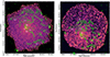 |
Fig. 2. Left: Chandra exposure-corrected, background (NXB + X-ray foreground and background) subtracted image of Nest. Right: XMM-Newton exposure-corrected, background (NXB + X-ray foreground and background + soft proton) subtracted image of Nest. Both of these images were created in the 0.6−4.0 keV energy band. The images have been Gaussian-smoothed with a σ = 3 pixels for better visualization. The LOFAR 144 MHz radio contours from Brienza et al. (2021) are shown in green. The contour levels used were 3, 10, 25, and 60 × σ, where σ = 154 μJy/beam and the beam size is 8.6″×4.3″. The different lobes have been marked on each figure. |
For Chandra, all level 2 event files were first reprojected to a common tangent point. Count images and exposure maps were created in the 0.6−4.0 keV band for each reprojected event file and then combined to produce the total counts and exposure map. Point sources were again detected with the help of wavdetect. The point sources were removed in all spectral analysis. We also removed them from all image analysis in Sects. 5 to 8.
Background images for individual reprojected stowed event files were created in the same energy band as observation images and were scaled to match the 9−12 keV band emission. Similar to our XMM background image, these “stowed” event file images were combined and used to obtain total NXB image.
We next determined the unresolved CXB flux for ACIS and EPIC observations (see Appendix C). We then created an X-ray background (XRB) image for each using the CXB flux and the galactic foreground flux from Table 2. For XMM, we also created a soft proton background image using methods discussed in Appendix D. All these images were combined to produce the total scaled background image for XMM (NXB + X-ray background and foreground + soft proton) and for Chandra (NXB + X-ray background and foreground). These total scaled background images were used to obtain background-subtracted, exposure-corrected images and were also used to create annular regions for spectral extraction. The exposure-corrected, background-subtracted images for the full FOV of Chandra are shown in the left panel of Figure 2.
3. Search for substructure in the X-ray images
We conducted a visual inspection of the X-ray images from Chandra and XMM-Newton to identify any correlations or anti-correlations with the radio emission, which could indicate that the radio lobes are interacting with and potentially disturbing the IGrM. The images, on first look, appear smooth, with no visual evidence of discontinuities. We determined the center of the X-ray emission by weighting counts in the Chandra image within a one arcmin radius from the approximate center identified visually:
where ci is the number of counts in the i-th pixel and Ri is a vector for the location of the pixel. Using this procedure, we obtained the X-ray center of Nest to be RA = 4:06:37.804, Dec = +30:22:35.351. This is in remarkable agreement (within an offset of ∼1 arcsec) with the optical centroid of MCG+05-10-007 (RA = 4:06:37.739, Dec = +30:22:34:769; Gaia Collaboration 2020, 2021)7.
To further probe whether any structures exist, we subtracted from the Chandra image a fitted spherically symmetric double-beta surface brightness model. We show this subtracted image in the left panel of Figure 3. We used a double-beta profile instead of a single-beta profile to better model the steepening of surface brightness profile below 20 kpc (see Figure B.1 and Brienza et al. 2021 supplementary information). The two beta models had the same center and the fits were done using Pyproffit v0.58 (Eckert et al. 2020). The best-fit values are provided in Appendix B, and fitted profiles are shown in Figure B.1. Before fitting, all the point-source pixels in the Chandra counts image were replaced with counts interpolated from a defined background region. This region was chosen as an annular ellipse with the inner radius equal to the source radius and the outer radius 50% larger. We used the CIAO tool dmfilth and method=POISSON to automate this task.
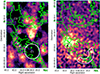 |
Fig. 3. Left: Chandra residual map after subtracting a spherically symmetric double beta model fit to the surface brightness profile of Nest. A depression near the C1 lobe can be seen in the image and has been highlighted as a circular region. A further possible depression may be present near the C2 lobe. The image has been heavily Gaussian-smoothed with a σ = 30″ and r = 30″ for better visualization. Right: XMM-Newton exposure-corrected image showing the region around the C1 lobe. The image has been Gaussian-smoothed with a σ = 6″ and r = 12″ for better visualization. A possible limb-brightened feature around the C1 lobe is shown in the figure as a wedge. The LOFAR radio contours from Figure 2 are shown in green. The X-ray center of the group has been marked with a cross in each figure. The different lobes have also been marked on each figure. |
As can be seen in Figure 3, no clear cavities are seen at the location of the A and B lobes with the present quality of data. However, we do identify a potential depression at the same location as the C1 radio bubble (Figure 3 left panel). This suggests that the radio jet from the AGN is likely displacing the X-ray-emitting gas and creating a cavity. We also noticed a potential limb-brightened region in the XMM exposure-corrected image near the C-lobe upon zooming in (Figure 3, right panel). This limb-brightened cavity was also detected by eROSITA (Brienza et al. 2021). We did not create any residual image for XMM due to the presence of a chip gap near the region of the C1 bubble.
We measure the enthalpy of this cavity and the temperature of the limb-brightened region in Section 7. There is also a hint of another depression at the location of the C2 bubble in both Chandra and XMM-Newton image, although this is difficult to confirm with the present quality of data. Current data quality also did not visually reveal any features corresponding to the D lobes and D2 filament, although there is an indication of a density break in this region (See Sect. 6). Any X-ray features that may be present in this region can help us to understand whether the filaments were created through a shock or as a consequence of the bubble evolution.
4. Spectral analysis
4.1. Region selection
We divided the fields of view of Chandra and XMM-Newton into annular bins with a constant signal-to-noise ratio. For Chandra, the net source count was chosen to be 1600 (SNR = 40). This SNR ensures a small statistical error (a few percent) on temperature profiles, while allowing enough spatial resolution to investigate whether the object has a cool core. This choice provides us with 11 bins with a bin width of 20−45 arcsec (7−16 kpc) over the field of view, with the outermost bin being 160 arcsec wide.
For XMM, we chose the annular regions such that each bin has a net source count of at least 3600 (SNR = 60). Due to XMM's higher sensitivity in the 0.6−4.0 keV band, a higher SNR threshold was chosen to investigate any temperature structures with better precision. At off-axis angles (>8 arcmin from the aimpoint; see Figure D.1), the source becomes faint due to the vignetting effect, and thus the soft protons become the dominant source of counts. Hence, we restricted the spectral extraction to 8 arcmin from the aimpoint. This choice resulted in 11 different annular bins with a bin width of 35−65 arcsec (13−24 kpc).
4.2. Spectral extraction and fitting
For XMM-Newton, we used the SAS tool evselect to extract spectra for each region from the observation, PN OoT, and FWC event files. The tasks rmfgen and arfgen were used to extract the redistribution matrix file (RMF) and the ancillary response file (ARF) for each region. To properly weigh the ARF, a detector map was provided for the extraction of such response files and the parameter extendedsource in arfgen was set to yes. For Chandra, the spectra from the observation and “stowed” event files, as well as RMF and ARF, were obtained with the CIAO tool specextract.
For XMM-Newton, the NXB spectrum in each region was modeled with a broken powerlaw and a set of delta and Gaussian functions. This helped us to fit the quiescent state and the fluorescent lines in the particle background spectrum. The X-ray background and foreground components obtained in Sect. 2.3 were used to model the soft-energy background emission. The normalization of each component was scaled to match the area of each annular extraction region. The PN OoT spectrum was fitted with a spline model with the particle background components held fixed. The soft proton contribution for each annulus was then determined (see Appendix D). While fitting the total spectra, all of the above components were held fixed. The IGrM was modeled using a single hot(cie) model in SPEX. In each annulus, spectra from MOS1, MOS2, and PN were fit simultaneously. The spectra were binned optimally in SPEX before fitting (Kaastra & Bleeker 2016). We used the C-statistic for minimization during fitting. The fit quality was generally found to be statistically acceptable. The C-statistic in the outermost bin of XMM was 424, while the expected C-statistic was 365±27. Any systematic uncertainty in the background estimate can contribute to a higher C-statistic due to the low flux in this bin. The C-statistic in the previous bin, by comparison, was 356, while the expected C-statistic was 362±27. The metallicity in the innermost three bins was allowed to vary, while it was kept fixed to a value of 0.2 in the other bins. This was done to ensure the metallicity value was not unconstrained during the fits. A value of 0.2 is consistent with similar metallicity values often seen in the outskirts of galaxy groups and clusters (Mernier et al. 2017).
While fitting Chandra spectra, the NXB and XRB components were also held fixed, and the IGrM component in each region was modeled with a hot(cie) model. The spectra from all ObsIDs were fitted simultaneously. The C-statistic in the outermost bin was 420, while the expected C-statistic was 360±30. All the fits were visually checked to confirm the absence of any systematic trends in the spectral residuals. A small systematic variation of the NXB between the stowed event files and the observed data may be responsible for the slightly higher-than-expected C-statistic. For the same reason as XMM-Newton fits, the metallicity was allowed to vary in the innermost bin, while it was kept fixed to 0.2 in the other bins. Chandra could only constrain metallicity in one bin since it has a lower effective area in the soft band9,10. This diminishes Chandra's ability to constrain the Fe-L complex at a temperature of a few keV.
5. Thermodynamic profiles
5.1. Temperature and metallicity
The temperature profiles along the radial direction, using data from both telescopes, are shown in the left column of Figure 4. We also show the outer edge of each pair of radio lobes in north and south directions with shaded regions. The robustness of the derived temperature values was tested by varying the normalization of the NXB, the galactic halo and the CXB. We find that the temperature value in the last bin is consistent within current statistical errorbars when the NXB normalization is varied up to 7% and the galactic halo, CXB normalization is varied up to a factor of 2. The systematic errors in our fits are thus smaller than the statistical errors.
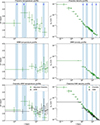 |
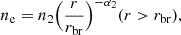
Fig. 4. Temperature profiles (left panel) and density profiles (right panel). First row: Chandra temperature and deprojected density profile as a function of projected radius. Second row: XMM-Newton temperature and deprojected density profile as a function of projected radius. Third row: Comparison between Chandra and XMM-Newton temperature and density profiles after taking into account systematics. The shaded regions show the extent of the four lobes shown in Figures 1 from the center of Nest. |
The Chandra temperature profile shows a tentative temperature drop (∼0.8 keV) below 30 kpc (80 arcsec), suggesting the group might have a cool core. In addition, there are hints of a slight temperature increase around 100 and 200 kpc (300 and 500 arcsec, respectively). This is also the distance of the C and D lobes from the center, as seen in the LOFAR images. The XMM measurements also suggest a temperature increase at a similar distance as the Chandra profile. However, the large errors in the temperature values prohibit us from concluding that there is a temperature jump at these locations. No temperature fluctuation is seen near the A and B lobes with the present quality of Chandra and XMM-Newton data.
Finally, in the bottom left panel of Figure 4, we show a comparison of the Chandra and XMM temperature profiles after taking into account the systematic differences. The scaling relationship describing the offset between Chandra and XMM-Newton temperatures can be written as (Schellenberger et al. 2015)
We used the full band (0.7−7.0 keV) best-fit values for the comparison between Combined XMM and ACIS-I (a = 0.889, b = 0) as there is very little emission in Nest beyond 4 keV. The error bars in the adjusted Chandra profile are larger than the original measurements because the statistical errors of the scaling parameters in Schellenberger et al. (2015) were taken into account as well. The adjusted Chandra temperatures are in agreement with those from XMM, except at the core, where the larger XMM bin is expected to smooth the underlying temperature structures.
Next, we turn our attention to the metallicity profile. As noted in Sect. 4.2, the abundance could only be constrained in the innermost bin of Chandra and the inner three bins of XMM. We show these derived metallicity values in Figure 5. As can be seen, XMM better constrains the abundance compared to Chandra. The measurements suggest that there may be a drop in metallicity in the core of the group.
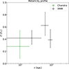 |
Fig. 5. Derived metallicity profiles from Chandra and XMM-Newton. The green data point is the Chandra value and the black data points are XMM-Newton values. Metallicity values beyond this region were assumed to be 0.2 solar during spectral fitting. |
5.2. Density
We also show deprojected density profiles from Chandra and XMM in Figure 4. The robustness of the derived density values was similarly checked as the temperature values. We again conclude that the effect of systematic uncertainty is lower than statistical uncertainty.
The deprojection of the density profile was done using the onion peeling method (Kriss et al. 1983) from surface brightness profiles in PyProffit. A constant temperature and metallicity of 2.1 keV and 0.3 Z⊙ were assumed to obtain the count rate to the emissivity conversion factor. The temperature of 2.1 keV corresponds to the XMM temperature in the innermost bin and is consistent with the temperature values throughout the field of view. We also found that the density values from PyProffit are mostly insensitive when the metallicity was varied between 0.2−0.4 Z⊙, i.e., the values within the central 20 kpc (see Figure 5). Any variation is within the current statistical error bars. Hence, we chose the median metallicity to obtain the density profiles. The spatial bins for density estimates were chosen such that each data point is at least 3σ significant. This criterion allows us to ensure that the errors are not too large due to the effects of onion deprojection, while at the same time ensuring a much more spatially resolved profile. We show this profile in the right column of Figure 4.
The higher resolved density profiles suggest certain interesting features at the location of the radio lobes. In the Chandra profile, near the location of the C lobe, we see a possible change in the slope of the profile (see Sect. 6 for a quantitative analysis). In the XMM profile, we see a possible density break at the location of the D lobe. No change in slope or density jumps are detected near the location of the A lobes. Near the B lobe, a small slope discontinuity can be visually seen in the Chandra data, but no such feature is seen in XMM. This feature can either be spurious, or XMM's bigger PSF smooths out this feature. In the bottom panel, we show a direct comparison of the Chandra and XMM profiles. We note that the Chandra profile reveals a steep density profile near the core with density values reaching 0.1 cm−3.
The aforementioned features could be related to either the northern or southern lobes or both. To investigate this, we also extracted density profiles along various azimuthal sectors with the same 3σ SNR. These profiles are shown in Figure 6. We also show the extraction regions for these profiles in the inset of each sub-figure. As the XMM profile is smooth in the inner regions and affected by the broader PSF, we only show the XMM profiles in these directions near the location of the C and D lobes.
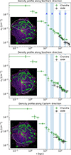 |
Fig. 6. Top: Density profile along the northern lobes. Middle: Density profile along the southern lobes. Bottom: Density profile along the eastern direction where there is no radio emission. The shaded regions show the extent of the four lobes shown in Figures 1 from the center of Nest. The inset figures show the extraction regions. |
We see that the jump near the D lobe is present in the northern direction, while the slope change near the C lobes is stronger in the southern direction (See Sect. 6 for fits). We note, though, that neither the Chandra nor XMM fields of view extend significantly beyond the edge of the southern D lobe. We also extracted the density profile along the eastern direction where there is no radio emission to check whether the density jumps are indeed due to the radio lobes. As expected, we do not see any density jump in this direction. These results suggest that the AGN may be responsible for disrupting the IGrM and may also be causing the temperature increase near C and D lobe locations (as discussed in Sect. 5.1).
5.3. Mass estimates
Brienza et al. (2021) reported a total X-ray mass of M500=(3−7)×1013 M⊙ using mass-temperature scaling relations. Using the density and temperature profile reported before, we provide here an estimate for M2500 and an updated M500. Under the assumption of hydrostatic equilibrium, the total mass can be calculated as
where μ is reduced mass factor with a value of 0.596, mp is the proton and G is the gravitational constant.
To compute the mass, we first fitted a parametric density and temperature model widely used in the literature (Vikhlinin et al. 2006) to the derived profiles. Since the parameters in Vikhlinin et al. (2006) model are highly degenerate, we only vary the parameters that could be constrained by our temperature and density profiles (see Sect. E). Using those parameters, we estimated M2500∼1.4×10¹³ M⊙ and M500∼3×10¹³ M⊙. The M2500 and M500 values correspond to R2500∼215 kpc and R500∼480 kpc, respectively.
With these values, we can also calculate the gas mass fraction, fg,500=Mgas/M:
where the gas density ρg = 2.3μmpnp and np=ne/1.21 is the proton number density. The factor of 2.3 is needed to convert proton number density to total number density according to the adopted abundance table from Lodders et al. (2009). We calculated fg,500∼4% at R500 by extrapolating our profiles. This value is typical of galaxy groups that are found in the literature (e.g., Gastaldello et al. 2007).
Independent mass estimate using eROSITA
We do note that the estimate of M500 discussed above was obtained by extrapolating our density and temperature profiles to R500. This was necessary because R500 of Nest is outside the field of view of both Chandra and XMM-Newton. This may lead to sizable systematic uncertainties in estimating M500. Hence, we also provide an independent estimate using the eROSITA data described in Brienza et al. (2021) that has larger field of view compared to Chandra and XMM-Newton. The density profile was independently measured by eROSITA from the center to 12 arcmin. The density outside XMM field of view was then approximated by a single beta model (Cavaliere & Fusco-Femiano 1976) with a norm ∼5×10⁻⁴ cm−3, rc∼4.9 arcmin and β∼0.494. With this density profile, and an assumed isothermal gas with an eROSITA measured temperature of 2.2 keV, we independently obtain M500∼7×10¹³ M⊙ and R500∼640 kpc. We note that, due to the fainter nature of the outskirts, systematic uncertainties on the level of the sky background can affect the outer slope of the eROSITA density profile, and hence the mass estimation. All mass estimates are reported in Table 3.
Mass estimates of Nest from Chandra, XMM-Newton, and eROSITA.
5.4. Pressure
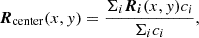
We show azimuthally averaged pressure profiles from Chandra and XMM in Figure 7 (top panel). The electron pressure was calculated using the formula

where ne is electron number density. We have corrected temperature systematics between Chandra and XMM before overplotting the pressure profile. To calculate the pressure profile, we used the higher resolved bins of the density profile. As the temperature profile is less resolved, we used the nearest temperature values to calculate the pressure value in each bin.
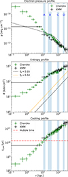 |
Fig. 7. Top: Azimuthally averaged electron pressure profiles. The average expected profile from Planck clusters is shown with a black dashed line. Middle: Azimuthally averaged entropy profile. The self-similar r1.1 profile for fb = 0.15 is shown with a black dashed line, while the fb = 0.04 profile is shown with an orange dashed line. Bottom: Radial profile of the cooling time obtained from azimuthally averaged density, temperature, and metallicity profiles. The Hubble time 1/H0 is shown in red. The shaded regions show the extent of the four lobes shown in Figures 1 from the center of Nest. |
We note that similar to the density and temperature profiles, there are slope changes and jumps near the locations of the C and D lobes. We further compared our pressure profile with a generalized profile available in the literature (Nagai et al. 2007):
![$$ \frac {p(r)}{p_{500}} = \frac {p_0}{(c_{500}x)^{\gamma } [1 + (c_{500}x)^{\alpha }]^{(\beta -\alpha )/\gamma }}, $$](/articles/aa/full_html/2025/07/aa54682-25/aa54682-25-eq7.gif)
where,
and x=r/r500. We used the best-fit parameter values from 62 clusters in Planck Collaboration Int. V (2013), [p0,c500,α,β,γ] = [6.41, 1.81, 1.33, 4.13, 0.31], to plot the black dashed line in the same figure. For our object, we obtain P500∼10−12 erg cm−3. The Planck pressure profile is similar to the pressure profile in the earlier work of Arnaud et al. (2010) (See Figure 4 of Planck Collaboration Int. V 2013 for a direct comparison). Although the generalized profiles are derived from clusters, Sun et al. (2011) showed that the median pressure profile of a sample of 43 nearby galaxy groups matches the Arnaud et al. (2010) universal profile well. Hence, in our work, we directly compare the pressure profile of our galaxy group object with the updated universal cluster profile from Planck Collaboration Int. V (2013).
The unusually steep density profile of our object may explain the deviation from the average expected profile at r<10 kpc. We do, however, observe that the pressure in our object is consistently below the average profile from 10−200 kpc. Beyond 200 kpc, the average profile is below what we find in Nest. Such a characteristic possibly suggests that gas is being removed from the location of the radio lobes and ejected to larger distances.
5.5. Entropy
The entropy profiles from Chandra and XMM are shown in Figure 7 (middle panel). The entropy was calculated using the formula

where ne is the electron number density.
We also plot the expected entropy from purely gravitational heating. This self-similar entropy profile (KSSC) was calculated following Voit et al. (2005) and Pratt et al. (2010):

with the self-similar normalization K500 given by
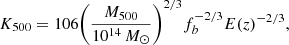
where fb is the baryon fraction and 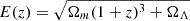 . For Nest, we obtain a K500 = 171 keV cm2. We calculated the self-similar entropy profile using a universal baryon fraction value of 0.15 as well as our measured baryon fraction of 0.04.
It is clear that the derived entropy is substantially higher than that from purely self-similar processes. Adopting a similar approach to Eckert et al. (2025), we used the expected self-similar entropy profiles to calculate the excess heat per particle (ΔQ) in the IGrM by assuming an isochoric process (neglecting any cooling losses; Finoguenov et al. 2008; Chaudhuri et al. 2012):
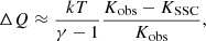
where γ = 5/3 is the adiabatic index and Kobs is the observed entropy from data. This is a lower limit on the non-gravitational heat energy since gas ejected from the halo is not taken into account. The total heat energy could then be calculated as
Using the above formulas, we obtained the total excess heat over the whole field of view, Qtot∼6.5×1060 erg for fb = 0.15. For fb = 0.04, we obtain Qtot∼5×1060 erg. At least some of this excess heat is likely attributed to the central AGN activity, although the exact contribution is difficult to quantify since some entropy excess might have already been in place during the pre-heating phase (see Figure 9 of McCarthy et al. 2011). We also note that the eROSITA mass estimate is higher (see Sect. 5.3). If we use the eROSITA gas density and a baryon fraction of 0.15, we obtain Qtot∼6.1×1060 erg.
5.6. Cooling time
The cooling time of a gas is defined as its thermal energy divided by the cooling rate. The cooling time, therefore, can be calculated as
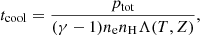
where ptot = 2.3p/1.21 is the total gas pressure, nH≈np=ne/1.21 is the hydrogen density, and Λ(T,Z) is the cooling function. We calculated the cooling function at each spatial bin from the temperature, metallicity and density profile shown in Figure 5. The radial dependence of the cooling times is shown in Figure 7 (bottom panel) along with the Hubble time 1/H0. It is clear that the gas below 10 kpc may cool within the Hubble time. In the central region, the cooling time is as low as ∼300 Myr. However, both the radio morphology of the source and the radio spectral aging analysis (Brienza et al. 2025) suggest a very rapid duty cycle for the jet activity, with active phases of 50–100 Myr and very short inactive phases in between. The AGN can thus heat the IGrM much faster than the time the gas takes to cool.
5.7. Binding energy versus excess heat
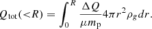
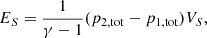
To investigate excess heating compared to gravitational binding energy Ebind, we estimated Ebind as
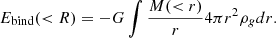
Figure 8 shows the excess heat in the form of excess entropy and the binding energy as a function of radius. We used the Chandra and XMM-Newton data up to the field of view to calculate these profiles. It is clear that in the inner regions of the group (<13 kpc), the excess heat is lower than the binding energy. This further suggests that the heating is insufficient to prevent the formation of a cool core and is consistent with the temperature drop we obtained from the Chandra profile. Beyond 13 kpc, the excess heat is higher, which may result in some gas being pushed out of the group towards the outskirts.
 |
Fig. 8. Energy budget of the IGrM of the galaxy group Nest. The orange line shows the heating due to excess entropy. The blue line shows the binding energy of the object obtained through Eq. (13). The black dashed line shows the location of R500 from Chandra and XMM-Newton data. |
6. Density breaks
In Sect. 5.2, we discussed a possible density slope change and density jump at the location of the C and D lobes. In this section, we aim to quantify the magnitude and significance of these breaks. In particular, we focus on two features: (1) the density slope change as seen in the Chandra data (Figure 6, middle panel) near the C lobe along the southern direction (2) the density jump as seen in the XMM-Newton data (Figure 4, middle right panel) near the D lobe in the azimuthally averaged profile. We chose the azimuthally averaged XMM profile instead of the northern or southern profile as they have insufficient counts near the D lobe to constrain the jump.
We fitted a broken powerlaw model to these density profiles to constrain the slope change and jump. This model can be expressed as
where rbr is the break distance, n1 is the density before the break and n2 is density after the break. α1 and α2 are the slope of the density profile before and after the break, respectively. The fits are shown in Figure 9.
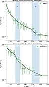 |
Fig. 9. Top: Azimuthally averaged XMM-Newton density profile. Bottom: Chandra density profile along the southern lobes. The sector used to extract this profile is shown in Figure 6 inset. The black lines show the fitted broken powerlaw model. The shaded regions show the extent of the C and D lobes from the center of Nest. |
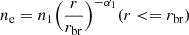
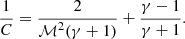
For the azimuthally averaged XMM density profile, at the edge of the D lobes, we obtained n1=(1.55±0.15)×10−4 cm−3, n2=(1.21±0.14)×10−4 cm−3. Defining the jump as C=n1/n2, we calculated a jump C = 1.27±0.19. This suggests a marginal 1.5σ deviation from a no-jump scenario (C = 1). If this jump is being created by a shock, the corresponding Mach number would be ℳ = 1.19±0.14. This can be obtained from C by (Sarazin 2002)
Such a Mach number is consistent with the values reported in the literature for objects with AGN-driven shocks (Forman et al. 2007; Simionescu et al. 2009; Randall et al. 2015; Snios et al. 2018). We also calculated the energy, presuming that this jump is due to a shock. This energy can be calculated as (David et al. 2001)
where p2,tot and p1,tot are pre- and post-shock total gas pressures and  is the volume enclosed by the shock. We calculated the shock location to be rbr = 218 kpc, and with this value, we estimated an energy of 8.6×1059 erg for the shock. This energy is consistent with that of shocks seen in group-scale objects (see Eckert et al. 2021 for a review). We note that the Chandra field of view does not extend much beyond 200 kpc. Hence, it is not possible to do a similar analysis using just Chandra data and compare that with the XMM analysis. In our calculation, we assume that the shock is spherically symmetric but note that this can be an overestimate if the shock propagates in a preferential direction.
We do note that although the present evidence for a shock is weak, Brienza et al. (2021, 2025) reported flattening of the radio spectral index at the location of the D2 filament with respect to the surrounding lobe emission, which might indicate re-acceleration or compression of particles − possibly due to a weak shock produced by more recent AGN outbursts. From Figure 6, it is clear that the X-ray jump is primarily in the northern direction, i.e., at the location of the D lobes. The X-ray-detected jump may thus be associated with this speculated weak shock. It is not possible to determine the direction of the shock at this location with present data quality.
For the Chandra density profile along the southern direction, we obtained α1 = 0.4±0.2 and α2 = 1.0±0.2. The uncertainties suggest that the significance of the slope change is 2.1σ. We note that the XMM density profile does not show any slope change at the same location, as can be seen in Figure 6. There are two possibilities: (a) The C lobe and the C1 cavity unfortunately lie very close to an intersection of chip gaps in all three EPIC detectors. This causes a lack of sensitivity in this region. (b) This may simply be a spurious feature in the Chandra data. Higher-quality data may confirm or rule out the presence of these features in the future. (c) The larger PSF of XMM may smooth out the feature in this region. (d) It could be due to systematic uncertainties due to deprojection because, at larger radii, the azimuthal coverage of Chandra and XMM is different. We conclude that the present data quality provides low confidence in the presence of slope change and density jumps at the location of the C and D lobes.
7. Cavity properties
7.1. Cavity detection
7.1.1. CAvity DEtection Tool
In Figure 3, we noticed a surface brightness depression in the Chandra residual image towards the southwest direction of the group. This was also detected by an analysis of the eROSITA data. To independently verify if this depression is significant, we applied the Cavity Detection Tool (CADET; Plšek et al. 2023) to images from both Chandra and XMM. The CADET tool was developed primarily to detect cavities in Chandra images. We used the broad-band (0.5−7.0 keV) image and probed it on the following size scales: 128, 256, 384, 512 and 640 pixels (1 pixel = 0.492 arcsec). We used a broad-band image instead of the 0.6−4.0 keV band because CADET was specifically trained to look for cavities in the broad-band, and the discrimination thresholds were tuned accordingly. Furthermore, our choice of scales was limited by the fact that the size of the CADET convolutional neural network was chosen to be 128 pixels. For XMM-Newton, only scales of 128 and 256 pixels (1 pixel = 4 arcsec) could be probed as our choices were limited by the field of view. We furthermore chose the default discrimination threshold of 0.4 to look for cavities (see Plšek et al. 2023 for details).
Based on the Chandra image, the CADET pipeline detected only a single X-ray cavity, which is co-spatial with the surface brightness depression C1 from Figure 3, and spatially co-aligned with the extended radio emission (Figure 3). We show this result in Figure 10. When applied to an XMM image, the pixels in the CADET prediction at the position of the alleged X-ray cavity were also activated. Nevertheless, the prediction contained several other false positive cavities of similar significance, and thus, the detection based on XMM-Newton data is non-conclusive. We note, however, that the CADET pipeline has not been trained for XMM images. All three XMM instruments also have chip gaps near the location of the cavity. These reasons could cause CADET to be less reliable in the case of XMM.
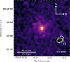 |
Fig. 10. Exposure-corrected Chandra image in the 0.5−7.0 keV band overlaid with the contours of CADET prediction (white and yellow contours correspond to values of 0.4 and 0.6, respectively). |
7.1.2. Azimuthal surface brightness analysis
We also checked the significance of the X-ray cavity using azimuthal surface brightness profiles. We calculated the depth (D) and significance of the cavity similarly as in Ubertosi et al. (2021):

where Sc and Ec represent the surface brightness and its uncertainty inside the C1 cavity region shown in Figure 3, SM and EM correspond to the median surface brightness and its uncertainty. In case the cavity region extends over multiple angular bins, SC and EC are calculated by adding the counts in all such bins. The median surface brightness was calculated in an angular region that is three times the angular extent of the cavity, excluding the cavity region. The radial width was chosen so that it covers the entire radial extent of the cavity. According to our definition, the depth represents the fractional decrement of surface brightness inside of the cavity compared to the median surface brightness.
We calculated the azimuthal surface brightness profile using a constant SNR of 15 for Chandra. This ensured we obtained a few bins inside the cavity region. For this choice, the depth and the significance in the Chandra image were found to be 24.3% and 2.6σ, respectively. The azimuthal surface brightness profiles are shown in Figure 11. The XMM image, on the other hand, showed a much weaker significance (∼1.6σ) as all three detectors had chip gaps near the cavity.
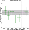 |
Fig. 11. Chandra azimuthal surface brightness profile (with SNR = 15) around the C1 cavity for 0.6−4.0 keV image. The extent of the cavity is shown with a black dashed line, while the median surface brightness is shown with a black dotted line. The error envelope for the median surface brightness is shown in black shaded region |
7.2. Cavity energetics
To measure the thermodynamic properties of the cavity, we extracted spectra from the region shown in Figure 3. We measure the temperature and density from the region in the same way as the thermodynamic profiles. We measure a temperature of  keV in the cavity region for Chandra and
  keV for XMM. Assuming an ellipsoidal geometry for the cavity, the volume can be calculated as V = 4πrarbrc/3, where (ra,rb) = (22,23) kpc for our extraction region. Since we do not have information about the dimension of the cavity along line-of-sight, we assume the length along this dimension to be the same as ra (i.e., rc=ra). With this volume, the enthalpy can be calculated using the following relation (for γ = 4/3, i.e., a relativistic gas):

The total gas pressure of the cavity was measured as  erg cm−3 for Chandra and
  erg cm−3 for XMM. From these pressure values, we obtained an enthalpy value of
  erg for Chandra and
  erg for XMM. The cavity is located at a projected distance of rcav = 50 kpc from the center, and thus the age of the cavity can be estimated as

where  is the local speed of sound. We calculated the sound speed and the corresponding sound travel time in each spatial bin using the temperature profile shown in Figure 4. We added the sound travel time from each bin to obtain the age of the cavity, tage. The sound speed in these bins varies between ∼770−870 km s−1. We estimated
  Myr for Chandra and
  Myr for XMM. Based on this, we calculated the cavity power as

For Chandra, the resulting power of the cavity is  erg s−1, while for XMM, it is
  erg s−1. We note that these values are upper limits since the distance to the cavity is measured in projected 2D space. We also used SPEX to calculate a luminosity of 8×1041 erg s−1 inside the cooling radius (r<20 kpc), i.e., the radius within which the cooling time is less than the Hubble time. Although the cavity is now present outside the cooling radius, it might have deposited energy within the cooling radius during expansion. Assuming such a scenario, the cavity power will be more than enough to offset radiative losses. The cavity power and cooling luminosity for this galaxy group are consistent with the upper range of the scatter found in the literature (e.g., Eckert et al. 2021; Hlavacek-Larrondo et al. 2022).
We further note that the cavity age was deduced higher in the Brienza et al. (2021) analysis for the cavities at the location of C lobes (tage,Brienza = 130 Myr). The higher age was calculated for a cavity at the location of C2 and using velocity dispersion of galaxies in the group (Tully 2015). An updated analysis based on spectral ageing suggests that the age of the C1 cavity can be as high as 160 Myr (Brienza et al. 2025). Brienza et al. (2021) also used an enthalpy of ptotV instead of 4ptotV while estimating the power of the cavity. An enthalpy of ∼ptotV is suitable for calculating the amount of energy already deposited by the cavity due to expansion while rising through the IGrM to its current position. On the other hand, an enthalpy of 4ptotV estimates the total energy that will be deposited by the cavity throughout the volume of the cluster. If we calculate the power of the cavity using the assumption of Brienza et al. (2021), i.e., Pcav=ptotV/tage,Brienza, we obtain Pcav∼6×1041 erg s−1. This is consistent with the 3×1041−1×1042 erg s−1 power range quoted in Brienza et al. (2021).
We also constrained the temperature of the bright rim around the cavity, as seen in the XMM-Newton image, to check if the expanding cavity is driving a shock into the IGrM. We find no discernible temperature jump that is expected from a shock. The temperature from Chandra was measured to be  keV and that from XMM was measured to be
  keV. This measurement is consistent with previous estimates using eROSITA.
8. The central supermassive black hole
8.1. Black hole mass
Using the temperature, cooling luminosity, gas mass fraction and power of the cavity, it is possible to obtain the central black hole mass, MBH, by using the scaling relations reported in Gaspari et al. (2019) and Plšek et al. (2022). These relations can be written as


where kTx,g and Lx,g are X-ray gas temperature and X-ray luminosity of the gas within 0.03R500∼14 kpc. We assume Pjet=Pcav for simplicity but note that Pcav may be an underestimate if a cavity in the direction opposite to C1 also exists, i.e., at the location of C2. We report the results from these relations in Figure 12. For black hole mass calculation, we used kTx,g=(2.5±0.2) keV, Lx,g=(8.2±0.7)×1041 erg s−1, fg,500∼0.04 and  erg s−1. These values were obtained in the previous sections.
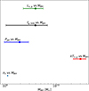 |
Fig. 12. Central black hole mass from scaling relations in Eqs. (21)–(24). The mass of the black hole estimated from Lx,g vs. MBH, Mg,500 vs. MBH, Pcav vs. MBH, kTx,g vs. MBH, and σv vs. MBH are (4±2)×109 M⊙, (4±3)×109 M⊙, (1.9±0.9)×109 M⊙, (30±9)×109 M⊙, and 1×10⁹ M⊙, respectively. |
It is clear from the figure that the mass estimates from Lx,g versus MBH, Mg,500 versus MBH, and Pjet versus MBH all agree with each other within 1.0−1.5σ. As noted, the black hole mass from Pjet is an underestimate if an X-ray cavity at the location of C2 also exists. However, the mass derived from kTx,g versus MBH disagrees with the others at 2.6−3.0σ level. This is very likely because Nest is very hot near the center compared to the objects in the sample of Gaspari et al. (2019). The hot core thus leads to an overestimate of the black hole mass and is an indication that the excess heat in Nest is high.
It is also possible to estimate the black hole mass from the expected stellar velocity dispersion. The circular velocity can be estimated as
where M is the mass and r is the distance from the center. Within central 10 kpc the gas pressure profile is well described by p(r)∝r−1 (see top panel of Figure 7) and the temperature T ≃ constant = 2.2 keV (see top panel of Figure 5). Thus, the mass M(r) is simply kTr/(μmpG) under the assumption of hydrostatic equilibrium. Then, M∝r and vcirc = constant = 590 km s−1 at r<10 kpc where the central galaxy dominates the gravitational potential. The stellar velocity dispersion σv profile thus strongly depends on a configuration of stellar orbits (e.g., Łokas & Mamon 2003). Still, there exists a radial range where σv only mildly depends on the anisotropy parameter which characterizes the orbital structure of a stellar system (see Churazov et al. 2010; Lyskova et al. 2014). According to Skrutskie et al. (2006), the central galaxy in Nest200047 is well described by a Sersic surface brightness profile with n = 4. For such an optical light profile the stellar velocity dispersion is weakly sensitive to the anisotropy parameter at r=(0.5−1)Reff (see Figure 3 in Churazov et al. 2010), where Reff is the effective (half-light) radius of a galaxy and Reff≃14″ as measured in Skrutskie et al. (2006). At these radii, i.e. at r≃7−14 arcsec, σv≃0.6vcirc≃350 km s−1. The obtained velocity dispersion estimate is slightly higher than the central velocity dispersion σc = 292.6±15.4 km s−1 measured within the inner r≲2″ (van den Bosch et al. 2015).
It is then possible to obtain a black hole mass using the well-known MBH−σv relation (e.g., Gebhardt et al. 2000; Ferrarese & Merritt 2000; Tremaine et al. 2002):
This relation was calibrated using the velocity dispersion measured within a slit extending to the effective radius of a galaxy, so we used the obtained above estimate of the velocity dispersion at r=(0.5−−1)Reff instead of the central value. For (α,β) = (8.13,4.02) (Tremaine et al. 2002), we obtain MBH∼1×10⁹ M⊙. This value is consistent (within 1.0−1.5σ) with estimates from Lx,g versus MBH, Mg,500 versus MBH, and Pcav versus MBH scaling relations.
8.2. Accretion power
The central galaxy MCG+05-10-007 lacks any strong optical emission lines and is thus classified as a Low Excitation Radio Galaxy (LERG; see supplementary information in Brienza et al. 2021). It has been argued in the literature that the LERGs accrete in a radiatively inefficient manner (e.g., Hardcastle et al. 2007; Janssen et al. 2012) that results from a geometrically thick flow, i.e., advection-dominated accretion flow (ADAF; Narayan & Yi 1995; Abramowicz et al. 1995). For such an accretion flow, the radiative efficiency of accretion can be very small (≤1 per cent), while the efficiency of the mechanical energy output remains high. Therefore, we first estimated the accretion efficiency of an idealized Bondi accretion (Bondi 1952) into the central black hole using the following relation (Churazov et al. 2002):
where s is the entropy, η is the accretion mechanical efficiency and LX is the cooling flow luminosity. This expression shows what gas entropy is needed to generate mechanical energy at a given rate via Bondi accretion. Using LX∼8×1041 erg s−1 (as reported in Sect. 7.2), the Chandra entropy value at the innermost radii (s∼10.9 keV cm2) and MBH∼1×10⁹ M⊙, we obtain η∼4.4×10⁻². The implicit assumption used here is that the gas radiative losses are compensated by the black hole the black hole output. The Bondi accretion rate is then
This mass accretion rate is a lower limit since the entropy at the Bondi accretion radius can be lower than the entropy at the innermost Chandra data point. The Bondi accretion power will be the same as the X-ray cooling luminosity according to our assumptions.
Observationally from the Chandra data, we find very little emission above 4.0 keV in the central region, suggesting that all of the observed emission is dominated by the diffuse thermal IGrM, with no evidence of non-thermal emission from a central point-like AGN in the X-rays. To estimate an upper limit to the central point-source flux, we fitted a single beta model to the surface brightness profile up to 10 arcsec (∼4 kpc) from the center in the 4.0−8.0 keV band. The obtained fitted parameters were: norm = (4±3)×10−5 photons s−1 cm−2 arcmin−2, rc = 2±2 arcsec and β = 0.5±0.3. We obtained the flux of the central point source by extrapolating the single beta model to the center (r = 0) and subtracting the model value from the flux in the central 2 pixel radius region (90% of the Chandra PSF11). From this calculation, we obtained a flux of (2±4)×10−8 photons s−1 cm−2 or a luminosity of (2±3)×1046 photons s−1 in the 4−8 keV band. For a powerlaw with a slope of Γ = 1.7 due to an X-ray corona in the central AGN, we calculate an upper limit on the 2−10 keV luminosity of L2−10keV=(3±6)×1038 erg s−1. Assuming a bolometric correction factor of ∼10 (Vasudevan & Fabian 2007), we estimated a 3σ upper limit of 2.1×1040 erg s−1 for the bolometric luminosity of the central black hole.
The above estimate suggests that the observed radiative power of the black hole is only ∼2.5% of the Bondi accretion power. Radiative power being much smaller than the accretion power has been previously reported in the literature for multiple objects, such as IC4296 (Pellegrini et al. 2003), M87 (Di Matteo et al. 2003), Centaurus A (Evans et al. 2004) and M84 (Bambic et al. 2023). Since Nest contains prominent radio jets and little nuclear emission, almost all of the accretion power is being converted into mechanical energy. This is physically plausible since ADAF accretion is known to direct the gravitational potential energy of the black holes into jets rather than radiative output (Narayan 2005; Ho 2008). We note that such an argument for low nuclear X-ray emission LERGs has been made previously in the literature (e.g., see Evans et al. 2006; Hardcastle et al. 2006, 2007).
9. Summary and conclusions
In this work, we have used 140 ks of Chandra and ∼25 ks of XMM-Newton data to study the Nest200047 (hereafter Nest) galaxy group that was detected by LOFAR. We aimed to study the effects of AGN feedback on the IGrM and the properties of the central black hole. In this work, we demonstrated that:
-
The thermodynamic profiles in Sect. 5 suggest that there is a cool core in Nest below 30 kpc as indicated by the temperature profile. The cooling profile further indicates that the cooling time at this distance is less than the Hubble time, and thus, the IGrM can form a cool core. Finally, the binding energy versus AGN heating profile suggests that the gravitational binding energy dominates the heating from the central AGN below ∼10 kpc, and thus, the energy provided by the AGN will be insufficient to prevent the formation of a cool core. All of these pieces of evidence suggest that Nest likely has a cool core within 10−30 kpc of the center.
-
Upon extrapolating the thermodynamic profiles and assuming a hydrostatic profile, we obtain a mass of (3−7)×1013 M⊙ within r500 using Chandra, XMM-Newton and eROSITA. This is consistent with the previously estimated mass reported in Brienza et al. (2021) using the mass-temperature scaling relation.
-
Past radio jet activity from the central AGN likely inflated a cavity in the IGrM as it can be visually seen in unsharp-masked Chandra images in Sect. 3. This cavity was also visually seen in the eROSITA data. Independent analysis using the CADET pipeline and azimuthal surface brightness analysis in Sect. 7.1 further corroborates this suggestion. The azimuthal profile analysis indicates a cavity significance of 2.6σ. The enthalpy of the cavity is estimated to be ∼1.4×1058 erg and the power is ∼7×1042 erg s−1. We conclude that this one cavity has more than enough power to offset radiative losses since the cooling luminosity is only ∼1042 erg s−1. However, more energy is likely being injected as there is evidence of multiple generations of bubbles in this system (Brienza et al. 2025).
-
We observe some density breaks in the density profile along the southern direction as well as in the azimuthally averaged profiles. The statistical significance of these breaks is between 1.5−2.1σ. We note that Brienza et al. (2021, 2025) detected flattening of the radio spectral index at the location of the D2 filament. It was speculated to be due to re-acceleration or compression of particles due to a weak shock produced by more recent AGN outbursts. Assuming the detected break near the D lobes is due to the speculated shock, we estimated an energy injection of 8×1059 erg in the IGrM assuming spherical geometry for the shock. If the shock exists, it would suggest that the dominant energy injection process is via shocks as opposed to energy deposition by cavities.
-
There is significant excess entropy in Nest as evidenced by the entropy profiles in Sect. 5. The total excess energy is estimated to be (5−6.5)×1060 erg depending on the assumed baryon fraction. The central AGN is likely responsible for some part of this energy. The energy from the central AGN is being added during an active phase of 50−100 Myr (Brienza et al. 2025).
-
The excess energy in the IGrM is higher than the binding energy above 13 kpc, suggesting that some gas can be pushed out of the object to the outskirts. There is some evidence of this in the pressure profiles in Figure 7. The pressure profile of our object is consistently below the average observed cluster pressure profile between 10−200 kpc. The total baryon fraction within r500 is estimated to be 4%. This fraction is typical for galaxy groups (Gastaldello et al. 2007).
-
From scaling relations, we obtain a central black hole mass of (1−4)×109 M⊙. The black hole mass derived from X-ray gas luminosity versus black hole mass, baryon fraction versus black hole mass, jet power versus black hole mass, and velocity dispersion versus black hole mass relation are consistent with each other within 1.0−1.5σ. However, the black hole mass obtained from X-ray gas temperature versus black hole mass relation is 2.6σ higher than that obtained from other relations. We argue that this is further evidence of the fact that the IGrM of Nest is super-heated, and this fact leads to a higher estimate of the black hole mass when using X-ray temperature.
-
The AGN at the center of Nest is very faint with a bolometric luminosity <2.1×1040 erg s−1 (3σ upper limit). The Bondi accretion calculations suggest that the total accretion power should be much higher, i.e., ∼8×1041 erg s−1. Thus, only ∼2.5% of the total accretion power is being channeled into radiative power. The rest of the energy is being channeled as jets instead. Such a scenario has been previously reported in the literature for accretion onto Low Excitation Radio Galaxies such as MCG+05-10-007 at the center of Nest200047.
The results of this work suggest that there is a large amount of excess heat in the IGrM of the Nest galaxy group, and the central AGN is likely responsible for some or most of this heating. In more massive objects (e.g., galaxy clusters), we know that the heating due to the AGN is typically a few times 1061 erg (e.g., McNamara et al. 2005; Wise et al. 2007; Majumder et al. 2024). The upper limit on the AGN energy output in Nest (6×1060 erg) is thus comparable to that seen in much more massive haloes. Due to the enormous excess heat, Nest could be part of a class of overheated galaxy groups such as ESO 3060170 (Sun et al. 2004), AWM 4 (Gastaldello et al. 2008), AWM 5 (Baldi et al. 2009) and SDSSTG 4436 (Eckert et al. 2025), where there is significant excess entropy and heating. The high star formation quenching in these objects indicates that Nest could be suffering a similar fate. Follow-up studies with optical and infrared data will be needed to confirm such a hypothesis.
Data availability
A copy of the reduced images is available at the CDS via anonymous ftp to cdsarc.cds.unistra.fr (130.79.128.5) or via https://cdsarc.cds.unistra.fr/viz-bin/cat/J/A+A/699/A375
The Chandra and XMM-Newton data used in this article are publicly available. All the codes and intermediate data products used to generate the results of this paper are publicly available at 10.5281/zenodo.15650741
Acknowledgments
This research has made use of data obtained from the Chandra Data Archive provided by the Chandra X-ray Center (CXC). We made use of NUMPY (van der Walt et al. 2011), SCIPY (Jones et al. 2001), ASTROPY (Astropy Collaboration 2013), and the SBFIT package (https://github.com/xyzhang/sbfit) (Zhang 2021) in this work. Plots were generated using MATPLOTLIB (Hunter 2007) and APLPY (https://github.com/aplpy/aplpy). AM thanks Elisa Costantini (SRON) and Liyi Gu (SRON) for discussions on the X-ray luminosity of the AGN at the center of Nest200047. TP thanks SRON for hosting his stay at the institute which enabled collaboration with AM and AS. The SRON Netherlands Institute for Space Research is supported financially by the Netherlands Organisation for Scientific Research (NWO). TP was supported by the GACR grant 21-13491X. M. Brienza acknowledges financial support from Next Generation EU funds within the National Recovery and Resilience Plan (PNRR), Mission 4 – Education and Research, Component 2 – From Research to Business (M4C2), Investment Line 3.1 – Strengthening and creation of Research Infrastructures, Project IR0000034 – “STILES – Strengthening the Italian Leadership in ELT and SKA”. M. Brüggen acknowledges funding by the Deutsche Forschungsgemeinschaft (DFG, German Research Foundation) under Germany's Excellence Strategy – EXC 2121 “Quantum Universe” – 390833306 and the DFG Research Group “Relativistic Jets”. IK acknowledges support by the COMPLEX project from the European Research Council (ERC) under the European Union's Horizon 2020 research and innovation program grant agreement ERC-2019-AdG 882679.
References
- Abramowicz, M. A., Chen, X., Kato, S., Lasota, J. -P., & Regev, O. 1995, ApJ, 438, L37 [NASA ADS] [CrossRef] [Google Scholar]
- Arnaud, M., Pratt, G. W., Piffaretti, R., et al. 2010, A&A, 517, A92 [CrossRef] [EDP Sciences] [Google Scholar]
- Astropy Collaboration (Robitaille, T. P., et al.) 2013, A&A, 558, A33 [NASA ADS] [CrossRef] [EDP Sciences] [Google Scholar]
- Ayromlou, M., Nelson, D., & Pillepich, A. 2023, MNRAS, 524, 5391 [CrossRef] [Google Scholar]
- Baldi, A., Forman, W., Jones, C., et al. 2009, ApJ, 694, 479 [Google Scholar]
- Bambic, C. J., Russell, H. R., Reynolds, C. S., et al. 2023, MNRAS, 522, 4374 [NASA ADS] [CrossRef] [Google Scholar]
- Begelman, M. C., & Cioffi, D. F. 1989, ApJ, 345, L21 [CrossRef] [Google Scholar]
- Best, P. N., Kaiser, C. R., Heckman, T. M., & Kauffmann, G. 2006, MNRAS, 368, L67 [NASA ADS] [Google Scholar]
- Biava, N., Brienza, M., Bonafede, A., et al. 2021, A&A, 650, A170 [NASA ADS] [CrossRef] [EDP Sciences] [Google Scholar]
- Bîrzan, L., Rafferty, D. A., McNamara, B. R., Wise, M. W., & Nulsen, P. E. J. 2004, ApJ, 607, 800 [Google Scholar]
- Bondi, H. 1952, MNRAS, 112, 195 [Google Scholar]
- Brienza, M., Shimwell, T. W., de Gasperin, F., et al. 2021, Nat. Astron., 5, 1261 [NASA ADS] [CrossRef] [Google Scholar]
- Brienza, M., Rajpurohit, K., Churazov, E., et al. 2025, A&A, 696, A239 [NASA ADS] [CrossRef] [EDP Sciences] [Google Scholar]
- Cash, W. 1979, ApJ, 228, 939 [Google Scholar]
- Cavaliere, A., & Fusco-Femiano, R. 1976, A&A, 49, 137 [NASA ADS] [Google Scholar]
- Chaudhuri, A., Nath, B. B., & Majumdar, S. 2012, ApJ, 759, 87 [NASA ADS] [CrossRef] [Google Scholar]
- Churazov, E., Forman, W., Jones, C., & Böhringer, H. 2000, A&A, 356, 788 [NASA ADS] [Google Scholar]
- Churazov, E., Sunyaev, R., Forman, W., & Böhringer, H. 2002, MNRAS, 332, 729 [NASA ADS] [CrossRef] [Google Scholar]
- Churazov, E., Tremaine, S., Forman, W., et al. 2010, MNRAS, 404, 1165 [NASA ADS] [Google Scholar]
- David, L. P., Nulsen, P. E. J., McNamara, B. R., et al. 2001, ApJ, 557, 546 [CrossRef] [Google Scholar]
- de Plaa, J. 2017, https://doi.org/10.5281/zenodo.2575495 [Google Scholar]
- DeGraf, C., & Sijacki, D. 2017, MNRAS, 466, 3331 [NASA ADS] [CrossRef] [Google Scholar]
- Di Matteo, T., Allen, S. W., Fabian, A. C., Wilson, A. S., & Young, A. J. 2003, ApJ, 582, 133 [NASA ADS] [CrossRef] [Google Scholar]
- Eckert, D., Finoguenov, A., Ghirardini, V., et al. 2020, Open J. Astrophys., 3, 12 [NASA ADS] [CrossRef] [Google Scholar]
- Eckert, D., Gaspari, M., Gastaldello, F., Le Brun, A. M. C., & O’Sullivan, E. 2021, Universe, 7, 142 [NASA ADS] [CrossRef] [Google Scholar]
- Eckert, D., Gastaldello, F., Lovisari, L., et al. 2025, A&A, submitted [arXiv:2506.13907] [Google Scholar]
- Evans, D. A., Kraft, R. P., Worrall, D. M., et al. 2004, ApJ, 612, 786 [NASA ADS] [CrossRef] [Google Scholar]
- Evans, D. A., Worrall, D. M., Hardcastle, M. J., Kraft, R. P., & Birkinshaw, M. 2006, ApJ, 642, 96 [Google Scholar]
- Fabian, A. C., Sanders, J. S., Taylor, G. B., et al. 2006, MNRAS, 366, 417 [NASA ADS] [CrossRef] [Google Scholar]
- Ferrarese, L., & Merritt, D. 2000, ApJ, 539, L9 [Google Scholar]
- Finoguenov, A., Ruszkowski, M., Jones, C., et al. 2008, ApJ, 686, 911 [NASA ADS] [CrossRef] [Google Scholar]
- Forman, W., Jones, C., Churazov, E., et al. 2007, ApJ, 665, 1057 [NASA ADS] [CrossRef] [Google Scholar]
- Fruscione, A., McDowell, J. C., Allen, G. E., et al. 2006, in Society of Photo-Optical Instrumentation Engineers (SPIE) Conference Series, eds. D. R. Silva, & R. E. Doxsey, SPIE Conf. Ser., 6270, 62701V [NASA ADS] [Google Scholar]
- Gaia Collaboration, 2020, VizieR On-line Data Catalog: I/350 [Google Scholar]
- Gaia Collaboration (Brown, A. G. A., et al.) 2021, A&A, 649, A1 [NASA ADS] [CrossRef] [EDP Sciences] [Google Scholar]
- Gaspari, M., Eckert, D., Ettori, S., et al. 2019, ApJ, 884, 169 [NASA ADS] [CrossRef] [Google Scholar]
- Gastaldello, F., Buote, D. A., Humphrey, P. J., et al. 2007, ApJ, 669, 158 [NASA ADS] [CrossRef] [Google Scholar]
- Gastaldello, F., Buote, D. A., Brighenti, F., & Mathews, W. G. 2008, ApJ, 673, L17 [NASA ADS] [CrossRef] [Google Scholar]
- Gebhardt, K., Bender, R., Bower, G., et al. 2000, ApJ, 539, L13 [Google Scholar]
- Gupta, Y., Ajithkumar, B., Kale, H. S., et al. 2017, Curr. Sci., 113, 707 [NASA ADS] [CrossRef] [Google Scholar]
- Hardcastle, M. J., Evans, D. A., & Croston, J. H. 2006, MNRAS, 370, 1893 [Google Scholar]
- Hardcastle, M. J., Evans, D. A., & Croston, J. H. 2007, MNRAS, 376, 1849 [NASA ADS] [CrossRef] [Google Scholar]
- Hlavacek-Larrondo, J., Li, Y., & Churazov, E. 2022, in Handbook of X-ray and Gamma-ray Astrophysics, eds. C. Bambi, & A. Sangangelo, 5 [Google Scholar]
- Ho, L. C. 2008, ARA&A, 46, 475 [Google Scholar]
- Huchra, J. P., Macri, L. M., Masters, K. L., et al. 2012, ApJS, 199, 26 [Google Scholar]
- Hunter, J. D. 2007, Comput. Sci. Eng., 9, 90 [NASA ADS] [CrossRef] [Google Scholar]
- Janssen, R. M. J., Röttgering, H. J. A., Best, P. N., & Brinchmann, J. 2012, A&A, 541, A62 [NASA ADS] [CrossRef] [EDP Sciences] [Google Scholar]
- Jonas, J., & MeerKAT Team, 2016, in MeerKAT Science: On the Pathway to the SKA, 1 [Google Scholar]
- Jones, E., Oliphant, T., & Peterson, P. 2001, SciPy: Open Source Scientific Tools for Python, http://www.scipy.org [Google Scholar]
- Kaastra, J. S. 2017, A&A, 605, A51 [NASA ADS] [CrossRef] [EDP Sciences] [Google Scholar]
- Kaastra, J. S., & Bleeker, J. A. M. 2016, A&A, 587, A151 [NASA ADS] [CrossRef] [EDP Sciences] [Google Scholar]
- Kaastra, J. S., Mewe, R., & Nieuwenhuijzen, H. 1996, UV and X-ray Spectroscopy of Astrophysical and Laboratory Plasmas, 411 [Google Scholar]
- Kaastra, J. S., Raassen, A. J. J., de Plaa, J., & Gu, L. 2018, https://doi.org/10.5281/zenodo.2419563 [Google Scholar]
- Kriss, G. A., Cioffi, D. F., & Canizares, C. R. 1983, ApJ, 272, 439 [Google Scholar]
- Kuntz, K. D., & Snowden, S. L. 2008, A&A, 478, 575 [NASA ADS] [CrossRef] [EDP Sciences] [Google Scholar]
- Lane, W. M., Clarke, T. E., Taylor, G. B., Perley, R. A., & Kassim, N. E. 2004, AJ, 127, 48 [NASA ADS] [CrossRef] [Google Scholar]
- Lehmer, B. D., Xue, Y. Q., Brandt, W. N., et al. 2012, ApJ, 752, 46 [NASA ADS] [CrossRef] [Google Scholar]
- Lodders, K., Palme, H., & Gail, H. P. 2009, Landolt-Börnstein, 4B, 712 [Google Scholar]
- Łokas, E. L., & Mamon, G. A. 2003, MNRAS, 343, 401 [NASA ADS] [CrossRef] [Google Scholar]
- Lyskova, N., Churazov, E., Moiseev, A., Sil’chenko, O., & Zhuravleva, I. 2014, MNRAS, 441, 2013 [Google Scholar]
- Majumder, A., Wise, M. W., Simionescu, A., & de Vries, M. N. 2024, MNRAS, 528, 1037 [Google Scholar]
- Marelli, M., Molendi, S., Rossetti, M., et al. 2021, ApJ, 908, 37 [CrossRef] [Google Scholar]
- McCarthy, I. G., Schaye, J., Bower, R. G., et al. 2011, MNRAS, 412, 1965 [Google Scholar]
- McNamara, B. R., & Nulsen, P. E. J. 2007, ARA&A, 45, 117 [NASA ADS] [CrossRef] [Google Scholar]
- McNamara, B. R., Wise, M. W., Nulsen, P. E. J., et al. 2001, ApJ, 562, L149 [NASA ADS] [CrossRef] [Google Scholar]
- McNamara, B. R., Nulsen, P. E. J., Wise, M. W., et al. 2005, Nature, 433, 45 [NASA ADS] [CrossRef] [PubMed] [Google Scholar]
- Mernier, F., de Plaa, J., Lovisari, L., et al. 2015, A&A, 575, A37 [NASA ADS] [CrossRef] [EDP Sciences] [Google Scholar]
- Mernier, F., de Plaa, J., Kaastra, J. S., et al. 2017, A&A, 603, A80 [NASA ADS] [CrossRef] [EDP Sciences] [Google Scholar]
- Morganti, R. 2017, Nat. Astron., 1, 596 [Google Scholar]
- Morganti, R. 2024, Galaxies, 12, 11 [NASA ADS] [CrossRef] [Google Scholar]
- Nagai, D., Vikhlinin, A., & Kravtsov, A. V. 2007, ApJ, 655, 98 [Google Scholar]
- Narayan, R. 2005, Ap&SS, 300, 177 [NASA ADS] [CrossRef] [Google Scholar]
- Narayan, R., & Yi, I. 1995, ApJ, 452, 710 [NASA ADS] [CrossRef] [Google Scholar]
- Pellegrini, S., Venturi, T., Comastri, A., et al. 2003, ApJ, 585, 677 [Google Scholar]
- Perley, R. A., Chandler, C. J., Butler, B. J., & Wrobel, J. M. 2011, ApJ, 739, L1 [Google Scholar]
- Planck Collaboration Int. V. 2013, A&A, 550, A131 [NASA ADS] [CrossRef] [EDP Sciences] [Google Scholar]
- Plšek, T., Werner, N., Grossová, R., et al. 2022, MNRAS, 517, 3682 [Google Scholar]
- Plšek, T., Werner, N., Topinka, M., & Simionescu, A. 2023, MNRAS, 527, 3315 [Google Scholar]
- Pratt, G. W., Arnaud, M., Piffaretti, R., et al. 2010, A&A, 511, A85 [NASA ADS] [CrossRef] [EDP Sciences] [Google Scholar]
- Predehl, P., Andritschke, R., Arefiev, V., et al. 2021, A&A, 647, A1 [EDP Sciences] [Google Scholar]
- Randall, S. W., Forman, W. R., Giacintucci, S., et al. 2011, ApJ, 726, 86 [NASA ADS] [CrossRef] [Google Scholar]
- Randall, S. W., Nulsen, P. E. J., Jones, C., et al. 2015, ApJ, 805, 112 [NASA ADS] [CrossRef] [Google Scholar]
- Rosas-Guevara, Y., Bower, R. G., Schaye, J., et al. 2016, MNRAS, 462, 190 [CrossRef] [Google Scholar]
- Sabol, E. J., & Snowden, S. L. 2019, sxrbg: ROSAT X-Ray Background Tool, Astrophysics Source Code Library, [record ascl:1904.001] [Google Scholar]
- Sarazin, C. L. 2002, in Merging Processes in Galaxy Clusters, eds. L. Feretti, I. M. Gioia, & G. Giovannini, Astrophys. Space Sci. Lib., 272, 1 [NASA ADS] [Google Scholar]
- Schellenberger, G., Reiprich, T. H., Lovisari, L., Nevalainen, J., & David, L. 2015, A&A, 575, A30 [NASA ADS] [CrossRef] [EDP Sciences] [Google Scholar]
- Schellenberger, G., David, L. P., Vrtilek, J., et al. 2021, ApJ, 906, 16 [Google Scholar]
- Shimwell, T. W., Tasse, C., Hardcastle, M. J., et al. 2019, A&A, 622, A1 [NASA ADS] [CrossRef] [EDP Sciences] [Google Scholar]
- Simionescu, A., Roediger, E., Nulsen, P. E. J., et al. 2009, A&A, 495, 721 [NASA ADS] [CrossRef] [EDP Sciences] [Google Scholar]
- Simionescu, A., ZuHone, J., Zhuravleva, I., et al. 2019, Space Sci. Rev., 215, 24 [NASA ADS] [CrossRef] [Google Scholar]
- Skrutskie, M. F., Cutri, R. M., Stiening, R., et al. 2006, AJ, 131, 1163 [NASA ADS] [CrossRef] [Google Scholar]
- Snios, B., Nulsen, P. E. J., Wise, M. W., et al. 2018, ApJ, 855, 71 [NASA ADS] [CrossRef] [Google Scholar]
- Snowden, S. L., Mushotzky, R. F., Kuntz, K. D., & Davis, D. S. 2008, A&A, 478, 615 [NASA ADS] [CrossRef] [EDP Sciences] [Google Scholar]
- Stuhlinger, M. 2008, Increased low energy noise below 1 keV or the MOS2CCD5 effect. Technical Report XMM-SOC-INST-TN-0033, Issue 1.1, ESA ESOC [Google Scholar]
- Sun, M., Forman, W., Vikhlinin, A., et al. 2004, ApJ, 612, 805 [Google Scholar]
- Sun, M., Sehgal, N., Voit, G. M., et al. 2011, ApJ, 727, L49 [NASA ADS] [CrossRef] [Google Scholar]
- Sunyaev, R., Arefiev, V., Babyshkin, V., et al. 2021, A&A, 656, A132 [NASA ADS] [CrossRef] [EDP Sciences] [Google Scholar]
- Tremaine, S., Gebhardt, K., Bender, R., et al. 2002, ApJ, 574, 740 [NASA ADS] [CrossRef] [Google Scholar]
- Tully, R. B. 2015, AJ, 149, 171 [NASA ADS] [CrossRef] [Google Scholar]
- Ubertosi, F., Gitti, M., Brighenti, F., et al. 2021, ApJ, 923, L25 [NASA ADS] [CrossRef] [Google Scholar]
- van den Bosch, R. C. E., Gebhardt, K., Gültekin, K., Yıldırım, A., & Walsh, J. L. 2015, ApJS, 218, 10 [Google Scholar]
- van der Walt, S., Colbert, S. C., & Varoquaux, G. 2011, Comput. Sci. Eng., 13, 22 [Google Scholar]
- Vantyghem, A. N., McNamara, B. R., Russell, H. R., et al. 2014, MNRAS, 442, 3192 [Google Scholar]
- Vasudevan, R. V., & Fabian, A. C. 2007, MNRAS, 381, 1235 [NASA ADS] [CrossRef] [Google Scholar]
- Vikhlinin, A., Kravtsov, A., Forman, W., et al. 2006, ApJ, 640, 691 [Google Scholar]
- Voit, G. M., Kay, S. T., & Bryan, G. L. 2005, MNRAS, 364, 909 [NASA ADS] [CrossRef] [Google Scholar]
- Werner, N., Simionescu, A., Million, E. T., et al. 2010, MNRAS, 407, 2063 [NASA ADS] [CrossRef] [Google Scholar]
- Werner, N., McNamara, B. R., Churazov, E., & Scannapieco, E. 2019, Space Sci. Rev., 215, 5 [CrossRef] [Google Scholar]
- Willingale, R., Starling, R. L. C., Beardmore, A. P., Tanvir, N. R., & O’Brien, P. T. 2013, MNRAS, 431, 394 [Google Scholar]
- Wise, M. W., McNamara, B. R., Nulsen, P. E. J., Houck, J. C., & David, L. P. 2007, ApJ, 659, 1153 [NASA ADS] [CrossRef] [Google Scholar]
- Zhang, X. 2021, https://doi.org/10.5281/zenodo.5507575 [Google Scholar]
- Zhang, X., Simionescu, A., Akamatsu, H., et al. 2020, A&A, 642, A89 [NASA ADS] [CrossRef] [EDP Sciences] [Google Scholar]
Appendix A: Soft X-ray noise in the EMOS1 spectrum
The fit for the innermost XMM bin is shown in Figure A.1. We used a hot(cie) + NXB + XRB + OoT spline model to fit the spectrum from MOS1, MOS2, and PN simultaneously. To avoid soft noise in MOS1, we neglected the MOS1 spectrum below 1 keV. The cstat of the 156, while the expected cstat is 136±17. Upon re-plotting the neglected part of the spectrum, we see that the MOS1 spectrum (blue) lies significantly above the model even though the MOS2 and PN spectrum agrees with the model. We speculate that this effect could be due to soft X-ray noise in the central CCD of MOS1 and is similar to what has already been reported in the literature for other MOS1 chips (Kuntz & Snowden 2008).
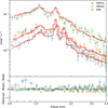 |
Fig. A.1. MOS1 (blue), MOS2 (orange), and PN (green) spectra in the innermost XMM bin fitted simultaneously with hot(cie) + NXB + XRB + OoT spline model. During the fit the MOS1 spectrum below 1 keV was neglected. |
Appendix B: Surface brightness fit parameters
The left panel of Figure 3 was obtained by subtracting a spherically symmetric double beta model:
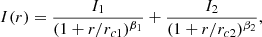
The fitted parameters, along with their errors, are shown in Table E.1. The Chandra and XMM-Newton surface brightness profiles are shown in Figure B.1 along with the fit to the Chandra profile. Each data point in the profiles is at least 3σ significant.
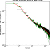 |
Fig. B.1. Chandra surface brightness profile is shown in green, while the XMM-Newton profile is shown in black. The fit to the Chandra profile used to obtain the left panel of Figure 3 is shown in red. |
Appendix C: CXB flux calculation
The XMM-Newton and Chandra observations of Nest has a deeper exposure compared to ROSAT all-sky data. Therefore, the CXB fluxes are lower as the telescopes can resolve more background point sources. To accurately determine the CXB flux, we first calculated the flux of point sources detected with wavdetect assuming a local background and using an exposure map. The point source exclusion limit was then obtained by creating a histogram of point source fluxes and choosing the flux for which the number of point sources is highest. We obtained a flux limit of 5×10⁻¹⁵ erg s−1 cm−2 in the 0.6−4.0 keV band for the Nest XMM observation. Assuming a logN-logS relation identical to the Chandra Deep Field South (Lehmer et al. 2012), we obtained the unresolved CXB flux value of (2.3±1.1)×10−15 erg s−1 cm−2 over a 1 arcmin2 area in the 2−8 keV range. This calculation was done using the publicly available software cxbtools12 (Mernier et al. 2015; de Plaa 2017). We find that this is ∼54% of ROSAT CXB flux in the same energy range. In terms of the pow model (see Section 2.3), a norm of 4.82×10⁻⁷ photons/s/cm2/keV for 1 arcmin2 sky area is appropriate for our case and has been used in all subsequent XMM analysis.
Following a similar procedure for Chandra, we obtain a point source exclusion flux limit of 8×10⁻¹⁶ erg s−1 cm−2 in the 0.6−4.0 keV band. This suggests an unresolved CXB flux of (1.2±0.3) ×10−15 erg s−1 cm−2 over a 1 arcmin2 area in the 2−8 keV range which is ∼30% of ROSAT CXB flux. Therefore, we used a pow norm of 2.63×10⁻⁷ photons/s/cm2/keV for 1 arcmin2 sky area in all subsequent Chandra analysis.
Appendix D: Soft proton calculation
As the XMM data is contaminated with soft protons at energies higher than a few keV, an accurate measure of soft proton flux was necessary to estimate IGrM temperatures. We thus extracted spectra from all XMM instruments in the 8−15 arcmin annulus centered at the aimpoint (see Figure D.1). These spectra were fit simultaneously in the 0.6−7.0 keV range. This wider energy range was chosen, as opposed to 0.6−4.0 keV, so that the soft proton contribution at higher energies is easier to constrain. We fit an absorbed cie to model the IGrM and a broken powerlaw to model the soft proton contribution. We ensured that the broken powerlaw model was not folded through the ARF. During the fit, non-X-ray background, PN OoT and X-ray background were held fixed. Among the broken powerlaw parameters, only the normalization was allowed to vary, while other parameter values were held fixed to the values obtained by Zhang et al. (2020) (see Appendix B.1). We fixed the metallicity of the cie model to 0.2 as well. The normalization of the soft proton for each instrument is reported in Table E.2. The cstat for this fit was 320, whereas the expected cstat was 260±20. The fit was visually checked to confirm the absence of any systematic residual. The soft proton contribution in any part of the CCD of any instrument can then be determined using the vignetting function described in Appendix B.2 of Zhang et al. (2020).
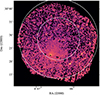 |
Fig. D.1. Region used for analyzing and fitting soft proton. The region extends from 8 to 15 arcmin from the aimpoint. |
Appendix E: Density and temperature fit parameters
The fitted parameters to the density and temperature model described in Vikhlinin et al. (2006) are noted in Tables E.3 and E.4. Only the values with errorbars could be constrained during the fit.
Best-fit parameters for the surface brightness profile.
SPEX broken power-law normalization values for EMOS1, EMOS2, and EPN instruments.
Best-fit parameters for density profile.
Parameters for the temperature profile.
All Tables
SPEX broken power-law normalization values for EMOS1, EMOS2, and EPN instruments.
All Figures
|
Fig. 1. LOFAR image of the galaxy group Nest200047, focusing on various spatial scales to highlight the four consecutive AGN outbursts detected in this system (Brienza et al. 2021). |
| In the text | |
|
Fig. 2. Left: Chandra exposure-corrected, background (NXB + X-ray foreground and background) subtracted image of Nest. Right: XMM-Newton exposure-corrected, background (NXB + X-ray foreground and background + soft proton) subtracted image of Nest. Both of these images were created in the 0.6−4.0 keV energy band. The images have been Gaussian-smoothed with a σ = 3 pixels for better visualization. The LOFAR 144 MHz radio contours from Brienza et al. (2021) are shown in green. The contour levels used were 3, 10, 25, and 60 × σ, where σ = 154 μJy/beam and the beam size is 8.6″×4.3″. The different lobes have been marked on each figure. |
| In the text | |
|
Fig. 3. Left: Chandra residual map after subtracting a spherically symmetric double beta model fit to the surface brightness profile of Nest. A depression near the C1 lobe can be seen in the image and has been highlighted as a circular region. A further possible depression may be present near the C2 lobe. The image has been heavily Gaussian-smoothed with a σ = 30″ and r = 30″ for better visualization. Right: XMM-Newton exposure-corrected image showing the region around the C1 lobe. The image has been Gaussian-smoothed with a σ = 6″ and r = 12″ for better visualization. A possible limb-brightened feature around the C1 lobe is shown in the figure as a wedge. The LOFAR radio contours from Figure 2 are shown in green. The X-ray center of the group has been marked with a cross in each figure. The different lobes have also been marked on each figure. |
| In the text | |
|
Fig. 4. Temperature profiles (left panel) and density profiles (right panel). First row: Chandra temperature and deprojected density profile as a function of projected radius. Second row: XMM-Newton temperature and deprojected density profile as a function of projected radius. Third row: Comparison between Chandra and XMM-Newton temperature and density profiles after taking into account systematics. The shaded regions show the extent of the four lobes shown in Figures 1 from the center of Nest. |
| In the text | |
|
Fig. 5. Derived metallicity profiles from Chandra and XMM-Newton. The green data point is the Chandra value and the black data points are XMM-Newton values. Metallicity values beyond this region were assumed to be 0.2 solar during spectral fitting. |
| In the text | |
|
Fig. 6. Top: Density profile along the northern lobes. Middle: Density profile along the southern lobes. Bottom: Density profile along the eastern direction where there is no radio emission. The shaded regions show the extent of the four lobes shown in Figures 1 from the center of Nest. The inset figures show the extraction regions. |
| In the text | |
|
Fig. 7. Top: Azimuthally averaged electron pressure profiles. The average expected profile from Planck clusters is shown with a black dashed line. Middle: Azimuthally averaged entropy profile. The self-similar r1.1 profile for fb = 0.15 is shown with a black dashed line, while the fb = 0.04 profile is shown with an orange dashed line. Bottom: Radial profile of the cooling time obtained from azimuthally averaged density, temperature, and metallicity profiles. The Hubble time 1/H0 is shown in red. The shaded regions show the extent of the four lobes shown in Figures 1 from the center of Nest. |
| In the text | |
|
Fig. 8. Energy budget of the IGrM of the galaxy group Nest. The orange line shows the heating due to excess entropy. The blue line shows the binding energy of the object obtained through Eq. (13). The black dashed line shows the location of R500 from Chandra and XMM-Newton data. |
| In the text | |
|
Fig. 9. Top: Azimuthally averaged XMM-Newton density profile. Bottom: Chandra density profile along the southern lobes. The sector used to extract this profile is shown in Figure 6 inset. The black lines show the fitted broken powerlaw model. The shaded regions show the extent of the C and D lobes from the center of Nest. |
| In the text | |
|
Fig. 10. Exposure-corrected Chandra image in the 0.5−7.0 keV band overlaid with the contours of CADET prediction (white and yellow contours correspond to values of 0.4 and 0.6, respectively). |
| In the text | |
|
Fig. 11. Chandra azimuthal surface brightness profile (with SNR = 15) around the C1 cavity for 0.6−4.0 keV image. The extent of the cavity is shown with a black dashed line, while the median surface brightness is shown with a black dotted line. The error envelope for the median surface brightness is shown in black shaded region |
| In the text | |
|
Fig. 12. Central black hole mass from scaling relations in Eqs. (21)–(24). The mass of the black hole estimated from Lx,g vs. MBH, Mg,500 vs. MBH, Pcav vs. MBH, kTx,g vs. MBH, and σv vs. MBH are (4±2)×109 M⊙, (4±3)×109 M⊙, (1.9±0.9)×109 M⊙, (30±9)×109 M⊙, and 1×10⁹ M⊙, respectively. |
| In the text | |
|
Fig. A.1. MOS1 (blue), MOS2 (orange), and PN (green) spectra in the innermost XMM bin fitted simultaneously with hot(cie) + NXB + XRB + OoT spline model. During the fit the MOS1 spectrum below 1 keV was neglected. |
| In the text | |
|
Fig. B.1. Chandra surface brightness profile is shown in green, while the XMM-Newton profile is shown in black. The fit to the Chandra profile used to obtain the left panel of Figure 3 is shown in red. |
| In the text | |
|
Fig. D.1. Region used for analyzing and fitting soft proton. The region extends from 8 to 15 arcmin from the aimpoint. |
| In the text | |
Current usage metrics show cumulative count of Article Views (full-text article views including HTML views, PDF and ePub downloads, according to the available data) and Abstracts Views on Vision4Press platform.
Data correspond to usage on the plateform after 2015. The current usage metrics is available 48-96 hours after online publication and is updated daily on week days.
Initial download of the metrics may take a while.