| Issue |
A&A
Volume 694, February 2025
|
|
|---|---|---|
| Article Number | A101 | |
| Number of page(s) | 17 | |
| Section | Interstellar and circumstellar matter | |
| DOI | https://doi.org/10.1051/0004-6361/202452827 | |
| Published online | 05 February 2025 | |
Circumstellar emission of Cepheids across the instability strip: Mid-infrared observations with VLTI/MATISSE★
1
Nicolaus Copernicus Astronomical Centre, Polish Academy of Sciences,
Bartycka 18,
00-716
Warszawa,
Poland
2
Université Côte d’Azur, Observatoire de la Côte d’Azur, CNRS,
Laboratoire Lagrange,
France
3
Instituto de Astrofísica, Departamento de Ciencias Físicas, Facultad de Ciencias Exactas, Universidad Andrés Bello,
Fernández Concha 700, Las Condes,
Santiago,
Chile
4
French-Chilean Laboratory for Astronomy, IRL 3386, CNRS,
Casilla 36-D,
Santiago,
Chile
5
LESIA, Observatoire de Paris, Université PSL, CNRS, Sorbonne Université, Université Paris-Cité,
5 Place Jules Janssen,
92195
Meudon,
France
6
European Southern Observatory,
Karl-Schwarzschild-Str. 2,
85748
Garching,
Germany
7
Universidad de Concepcion, Departamento de Astronomia,
Casilla 160C,
Chile
★★ Corresponding author; This email address is being protected from spambots. You need JavaScript enabled to view it.
Received:
31
October
2024
Accepted:
10
December
2024
Abstract
Context. The circumstellar envelopes (CSE) of Cepheids are still only poorly characterized despite their potential impact on the distance determination via both the period-luminosity relation and the parallax-of-pulsation method.
Aims. This paper aims to investigate Galactic Cepheids across the instability strip in the mid-infrared with MATISSE/VLTI in order to constrain the geometry and physical nature (gas and/or dust) of their CSEs.
Methods. We secured observations of eight Galactic Cepheids with short- and up to long-period pulsations with MATISSE/VLTI in the L, M, and N bands. For each star, we calibrated the flux measurements to potentially detect the spectral dust signature in the spectral energy distribution (SED). We then analyzed the closure phase and the visibilities in L, M, and N bands. The parallax-of-pulsation code SPIPS was used in order to derive the infrared excess and the expected angular stellar diameter at the date of the MATISSE observations. We also computed test cases of a radiative transfer model of dusty envelopes with DUSTY to compare them with the visibilities in the N band.
Results. The SED analysis in the mid-IR confirmed the absence of a spectral dust signature for the entire star sample. For each star, we observed closure phases in the L, M, and N bands that are consistent with a centro-symmetric geometry for the different targets. Finally, the visibilities in the L, M, and N bands agree with the expected angular stellar diameter. Although we did not resolve any circumstellar emission, the observations are compatible with the presence of compact CSEs within the uncertainties. We provide 2 σ upper limits on the CSE flux contribution based on model residuals for several CSE radii, which exclude models that are simultaneously large and bright (RCSE ≈ 10 R⋆ and fCSE ≈ 10%) for all the stars of the sample. Last, the visibilities in the N band rule out CSE models with optical depth τV ≳ 0.001 for different types of dust.
Conclusions. The MATISSE observations of eight Cepheids with different pulsation periods (from 7 to 38 days) and evolution stages provide a comprehensive picture of Cepheids from mid-infrared interferometry for the first time. We present additional evidence that circumstellar dust emission is negligible or absent around Cepheids for a wide range of stellar parameters in the instability strip. Further interferometric observations in the visible and near-infrared are required to separate the star and CSE, which is crucial for constraining the CSE contribution and its possible gaseous nature.
Key words: methods: observational / techniques: interferometric / circumstellar matter / stars: variables: Cepheids
Based on observations made with ESO telescopes at Paranal observatory under program 104.D-0554(B), 106.21RL.001, 106.21RL.002, and 106.21RL.003.
© The Authors 2025
 Open Access article, published by EDP Sciences, under the terms of the Creative Commons Attribution License (https://creativecommons.org/licenses/by/4.0), which permits unrestricted use, distribution, and reproduction in any medium, provided the original work is properly cited.
This article is published in open access under the Subscribe to Open model. This email address is being protected from spambots. You need JavaScript enabled to view it. to support open access publication.
1 Introduction
Cepheids demonstrate a well-known relation between their luminosity and pulsation period. This is commonly referred to as the period-luminosity (PL) relation and was famously recognized as the Leavitt law (Leavitt 1908; Leavitt & Pickering 1912). The PL relation was first applied to prove the extragalactic nature of spiral nebulae (Hubble 1925, 1926, 1929b) and then led to the discovery of the expansion of the Universe as characterized by the Hubble-Lemaître constant H0 (Lemaître 1927; Hubble 1929a). The extragalactic distance scale, which largely relies on the Cepheid PL relation, coupled with the observation of extragalactic Cepheids with the Hubble Space Telescope, yielded a precise determination of the accelerated expansion of the Universe (Riess et al. 2022).
However, the calibration of the PL relation is still affected by uncertainties at the percent level, and it is one of the largest contributors to the error budget on the Hubble–Lemaître constant H0 (Riess et al. 2022, 2024b). Despite evidence of infrared (IR) emission from the circumstellar envelope (CSE) of Cepheids, its impact as a possible bias or dispersion on the PL relation has not yet been taken into account, or was assumed to be negligible in the near-IR bands (Valentino & Brout 2024; Anderson 2024). The physical nature of the CSE emission is still poorly constrained, and therefore, no satisfying model of the spectral energy distribution (SED) is currently available. Moreover, the presence of CSEs around Cepheids, which might depend on fundamental stellar parameters, remains to be understood. This is of paramount importance to ensure that no systematic errors are introduced into the PL relation, and, consequently, into the measurement of H0. The need for a distance scale that is free from systematics is essential in the era of the James Webb Space Telescope (JWST), which is currently observing Cepheids in distant galaxies to refine the extragalactic distance scale (Freedman & Madore 2024; Riess et al. 2024a). Several studies have shown the potential impact of CSE emission on the PL relation so far (Neilson et al. 2009, 2010) and on the Baade-Wesselink (BW) method for deriving individual distances of Cepheids (Mérand et al. 2007, 2015; Gallenne et al. 2021; Nardetto et al. 2023; Hocdé et al. 2024b). Therefore, it is essential to understand the CSE characteristics as a function of the Cepheid properties to correct possible biases on photometric measurements.
Moreover, the circumstellar material can provide valuable insights into the mass-loss history of Cepheids. This is particularly significant within the context of the mass discrepancy observed in Cepheids, where the derived stellar masses can exhibit discrepancies of up to 20% when compared to pulsation models, such as those discussed in Caputo et al. (2005); Bono et al. (2006); Keller (2008), and dynamical mass measurements, as outlined in Pietrzyński et al. (2010). The first attempts to detect traces of mass loss were provided by mid- and far-IR photometric and imaging observations with the Infrared Astronomical Satellite (McAlary & Welch 1986; Deasy & Butler 1986; Deasy 1988) and later with Spitzer and Herschel (Neilson et al. 2009; Marengo et al. 2010a,b; Barmby et al. 2011; Gallenne et al. 2012; Hocdé et al. 2020b). Radio observations using the HI 21 cm line emission with the Very Large Array also revealed an extended gas environment around δ Cep and T Mon (Matthews et al. 2012, 2016). However, with the exception of a few cases in which Cepheids are embedded in large and cold interstellar dust material (e.g., RS Puppis and SU Cas), these observations have shown that an extended dusty environment can be excluded for the vast majority of Cepheids.
Another method for identifying IR excess from CSEs involves the comparison of observations with static atmosphere models. Several studies consistently reported a lack of substantial observational support for IR excess in a significant population of Cepheids (Schmidt 2015; Groenewegen 2020; Groenewegen & Lub 2023). However, these studies used mean photometry along the pulsation cycle, which might be problematic when the aim is to detect an IR excess of a few percent compared to the photosphere or a variable CSE emission. In contrast, Gallenne et al. (2012) interpolated photometric data to the specific phase of mid-IR observations to fit a consistent atmosphere model. They found an IR excess for most of the Cepheid in their sample. In order to achieve a sufficiently high precision, the parallax-of-pulsation code SpectroPhoto-Interferometric modeling of Pulsating Stars (SPIPS, Mérand et al. 2015) is well-suited for detecting subtle IR excesses because it can adjust atmosphere models throughout the pulsation cycle and aligns them with an extensive array of observations. In particular, Gallenne et al. (2021) demonstrated that fitting a CSE model in the parallax-of-pulsation model SPIPS significantly improved the goodness-of-fit for 13 out of 45 Cepheids. Notably, they found that these CSE models presented a mean excess of 0.08±0.04 mag in the K band (λ = 2.2 μm).
The high angular resolution provided by long-baseline interferometry is ideal to directly resolve the emission that extends for only several radii of the Cepheids. The first CSE was resolved for the first time in the K band based on data obtained with the Very Large Telescope Interferometer (VLTI/VINCI) around ℓ Car (Kervella et al. 2006), then around Polaris, δ Cep, and Y Oph at the Center for High Angular Resolution Astronomy (CHARA/FLUOR) (Kervella et al. 2006; Mérand et al. 2006, 2007). In the K band, the diameter of the envelope appears to be at least two stellar radii, and the flux contribution is up to 5% of the continuum. A similar result was achieved in the L band (3.5 μm) around ℓ Car (Hocdé et al. 2021) with VLTI/MATISSE. CSEs were also resolved in the N band (10 μm) around four Cepheids with VLTI/VISIR and VLTI/MIDI (Kervella et al. 2009; Gallenne et al. 2013). Interestingly, a CSE was also resolved in the visible band with the CHARA/VEGA instrument around δ Cep (Nardetto et al. 2016).
The size of CSEs directly relates to their nature, which was first assumed to be dusty. Several radiative transfer studies were based on this assumption (Gallenne et al. 2013; Groenewegen 2020; Hocdé et al. 2020b; Groenewegen & Lub 2023). Cepheids with long pulsation periods might have a dusty envelope, as expected based on their unusual chemical composition (Kovtyukh et al. 2024). However, near-IR emission and a CSE close to the star suggest an environment that is too hot for dust condensation, with temperatures exceeding 2000 K. These CSEs are likely to be composed of ionized gas that emits continuous free-free emission, as outlined by radiative transfer models (Hocdé et al. 2020b). This region might be linked to the chromospheric activity of the star, for which the radius was derived to be about Rchromo = 1.50 R⋆ (Hocdé et al. 2020a). The hot gas at a few stellar radii above the photosphere might be caused by pulsation-driven shocks (Fokin et al. 1996; Neilson et al. 2011; Moschou et al. 2020; Fraschetti et al. 2023).
Further observations are needed to constrain the size of the CSE, which is essential for modeling the physical process at play. While the first interferometric detections suggested a potential correlation between envelope emission and the pulsation period (Mérand et al. 2007), recent photometric analyses showed that the IR emission is not correlated to the pulsation period or the evolutionary stage of the Cepheid (Gallenne et al. 2021). We expect, however, that the efficiency of the mass-loss mechanism does depend on the Cepheid characteristics, as shown by Neilson & Lester (2008), especially in the case of pulsation-driven mass loss, because the shock intensity and the surface gravity must play a significant role.
In this paper, we report the study of CSE characteristics of eight Cepheids in the L (2.8–4.0 μm), M (4.5–5 μm), and N bands (8–13 μm) based on data obtained with the Multi AperTure mid-Infrared SpectroScopic Experiment (VLTI/MATISSE, Lopez et al. 2014; Allouche et al. 2016; Robbe-Dubois et al. 2018; Lopez et al. 2022). To this end, we observed Cepheids with different pulsation periods across the instability strip: X Sgr (7.01 d), U Aql (7.02d), η Aql (7.17d), β Dor (9.84 d), ζ Gem (10.15 d), TT Aql (13.75 d), T Mon (27.03 d), and U Car (38.87 d).
In the following, we first present the observations, the data reduction, and the calibration process of VLTI/MATISSE data in Sect. 2. From the MATISSE data alone, it is not possible to disentangle the Cepheid and the CSE because we do not resolve the stars up to the first null of the visibility function, which is essential for accurately determining the stellar angular diameter. Instead, we model the Cepheid photosphere along the pulsation cycle in Sect. 3 in order to derive the expected visibilities and flux of each star at the specific date of the MATISSE observations. Then, we successively study the calibrated flux in Sect. 4, the closure phase in Sect. 5, and the squared visibilities in Sect. 6. We discuss and summarize our results in Sect. 7.
Standard star properties for visibility and flux.
2 VLTI/MATISSE interferometric observations
MATISSE operates as the beam combiner for the L, M, and N bands within the VLTI facility at the Paranal Observatory. The VLTI comprises a combination of four 1.8-meter auxiliary telescopes (ATs) or four 8-meter unit telescopes (UTs), which offer an array of baseline lengths spanning from 11 meters to 150 meters. As a spectro-interferometer, MATISSE captures both dispersed fringes and spectra. MATISSE employs a standard observing mode known as the “hybrid” mode, which incorporates two distinct photometric measurement methods. For the L and M bands, it uses SIPHOT to simultaneously measure photometry alongside the dispersed interference fringes. Conversely, for the N band, it employs HIGH SENS to measure photometric flux independently after the interferometric observations.
The observational campaign was conducted between 2020 and 2022 during open and guaranteed time observation (GTO; T Mon was part of this program). These observations were executed using the UT quadruplet, resulting in ground baseline lengths ranging from 58 to 132 meters. Observations with UTs are required to observe in the N band since the flux of the brightest Cepheids is only a few Jansky. The log of the MATISSE observations is given in Table A.1.
We processed the raw data using the most recent version of the MATISSE data reduction software (DRS) version 2.0.2, which is publicly available1. The data reduction steps were explained in detail in Millour et al. (2016). The MATISSE absolute visibilities are estimated by dividing the measured correlated flux by the photometric flux. In our subsequent analysis, we excluded the 4.0 to 4.5 μm spectral region, where the atmosphere is not transmissive, and also the noisy edges of the atmospheric spectral bands (which might differ slightly from one star to the next). Thus, we analyzed the following spectral region in L (3.1–3.9 μm), M (4.5–4.9 μm), and N (8.1–12 μm) for the absolute visibility and flux. The only exception was U Aql, for which we acquired the correlated flux in the N band.
2.1 Atmospheric conditions
In the L and M bands, the brightness of the Cepheids sample (around 10 Jy) significantly exceeds the UT sensitivity in low-resolution mode (approximately 0.1 Jy), even in suboptimal atmospheric conditions. In contrast, under the most adverse conditions, atmospheric factors could impact the visibility of the faintest targets in the N band. As stated by Petrov et al. (2020), the coherence time has the most significant impact on the instrumental visibility. Consequently, caution is required for a coherence time shorter than 4 ms, in particular, for X Sgr in our sample (τ0 ≈ 2 ms), and therefore, we do not display its visibilities. Moreover, according to Lopez et al. (2022), the seeing-dependent Strehl ratio in the L band dominates the visibility calibration errors, while in the N band, as in MIDI, MATISSE is sensitive to the temporal fluctuations of the thermal background. Overall, our star sample was observed under excellent conditions with a seeing below 0.8 arcsecond and a coherence time τ0 > 4 ms (see Table A.1).
2.2 Choice of calibrators
For most of the Cepheids, two calibrators were observed in order to ensure a reliable calibration in the L, M and N bands (see Table A.1). We chose calibrators whose flux was comparable to that of scientific targets in the L and N bands, that is, ≈10 to 1 Jy, respectively, as shown in Table 1. These flux requirements induced the use of partially resolved calibrators at the 132 m longest baseline. Calibrators were selected using the Search-Cal tool of the JMMC2 with a high confidence level on the derived angular diameter (χ2 ≤ 5; see Appendix A.2 in Chelli et al. 2016). We also ensured that these calibrators were free from any IR emission flags as defined in the mid-IR stellar diameter and flux compilation catalog (MDFC, Cruzalèbes et al. 2019). The two calibrators of T Mon, namely 30 Gem and 18 Mon, were chosen in order to consistently compare the results with previous observations with VLTI/MIDI (Gallenne et al. 2013, hereafter G13). The L-band uniform disk (UD) angular diameters for the standard stars as well as the corresponding L- and N-band fluxes and the spectral types are given in Table 1. Last, we selected calibrators with a relatively small angular separation from the Cepheid (<15 degrees) in order to ensure a similar sky and instrumental transmission function, as well as a similar airmass for a reliable flux calibration.
After the calibrator observations, we verified the consistency of their angular diameter with values from the JSDC catalog (Bourgés et al. 2014). This is important for investigating possible systematic effects on the angular diameter measurements of the Cepheid. To this end, we followed the method employed by Robbe-Dubois et al. (2022). The observed difference between the fitted angular diameter θfit and the angular diameter from the JSDC θJSDC in the L band is indicated in Table A.1. In all cases, we find a difference lower than 5%, which allowed us to accurately calibrate the Cepheid visibilities.
3 Accurate stellar photosphere modeling with SPIPS
3.1 SPIPS modeling of the star sample
As outlined in the introduction, we need an accurate model of the photosphere and distance of the Cepheid in order to compare them with the MATISSE flux and angular diameter measurements. For this purpose, we used SPIPS introduced by Mérand et al. (2015), which enabled us to interpolate the atmosphere model of the Cepheids over the observations along the pulsation cycle. The principle of this parallax-of-pulsation code is based on the BW method (Baade 1926; Wesselink 1946). In this method, the distance is derived by comparing the variation in the radius and the angular diameter. The radius variation is derived from the pulsation velocity of the star by the mean of radial velocity measurements and the assumption of the projection factor (p-factor, see Nardetto et al. 2023, and references therein). On the other hand, the angular diameter variation is measured from interferometry or based on the surface brightness through the empirical surface brightness color relation (SBCR).
In contrast to the classical BW method, which derives the angular diameter using the SBCR in only two photometric bands, SPIPS is a sophisticated version that includes photometric, interferometric, effective temperature, and radial velocity measurements in a robust all-at-once model fit. Assuming a quasi-static photosphere of the Cepheids, it makes use of atmospheric ATLAS9 models from Castelli & Kurucz (2003), with solar metallicity and a standard turbulent velocity of 2 km/s, to fit observational data throughout the pulsation cycle. SPIPS was used in different studies that included Cepheids and RR Lyrae stars (Breitfelder et al. 2016; Gallenne et al. 2017; Hocdé et al. 2020b; Trahin et al. 2021; Gallenne et al. 2021; Bras et al. 2024).
Since SPIPS is a parallax-of-pulsation code, we must fix either the distance or the p factor, which are fully correlated. We adopted Gaia DR3 parallaxes (Gaia Collaboration 2016; Gaia Collaboration 2022) only in the case of TT Aql and U Car because they met the parallax quality criterion defined as Renormalised Unit Weight Error (RUWE) below 1.4, and do not saturate the detector with G > 6 mag. For these two stars, we also corrected the parallax by the Gaia zeropoint3 (Lindegren et al. 2021). For all other stars, we fixed the p factor to 1.27 following the mean values obtained for Cepheids (Trahin et al. 2021), and we adjusted the distance. We note that fixing either the distance or the p factor has no influence on the accuracy of the angular diameter and flux level, which are well constrained by the interferometric and photometric observations. For each star, we retrieved the radial velocity, effective temperature, angular diameter, and photometric measurements in various bands. The PIONIER interferometric observations in the H band (1.65 μm) that are available for most of the stars in our sample allowed us to constrain the angular stellar diameter tightly. We did not collect extensive photometric datasets, but instead used data from common sources whenever possible. Ideally, datasets must be obtained from the same instrument and observed during a short time-baseline to avoid any bias when applying the BW method (Wielgórski et al. 2024; Zgirski et al. 2024). This approach also ensured that the overall SPIPS fitting and IR excess measurements for different stars were more easily comparable.
In the case of U Aql, a special correction was needed since it is a known spectroscopic binary with an orbital period of 1862.8±1.1 day (Hocdé et al. 2024a). We corrected the radial velocity measurements for orbital motion following Gallenne et al. (2018, 2019). In our star sample, X Sgr, η Aql, β Dor, and ζ Gem represent the most complete datasets. We present the SPIPS results of η Aql and X Sgr in Fig. 1 and those for the other stars in Appendix B, together with the source of the observations used in Table B.2. Although we assumed different p factors and used different datasets, our SPIPS fitting agrees well with previous work from Trahin et al. (2021) and Gallenne et al. (2021) (see Table B).
3.2 Modeling the IR excess
SPIPS also takes into account the presence of CSE to model the synthetic photometry and interferometric observations from different instruments. As shown by Gallenne et al. (2021), the introduction of a parametric CSE model significantly improves the fitting of the SPIPS model for a large number of Cepheids. In our sample, the impact of the CSE for X Sgr and η Aql can be seen from interferometric observations, as shown in the angular diameter panels for each star in Fig. 1. This model consists of an IR excess modeled by a parametric power law. We instead employed a logistic function with two degrees of freedom to model the IR excess analytically, as proposed by Hocdé et al. (2024b). This is based on physical justifications of ionized gas CSE around the star and led to a spectral index of S ν ∝ ν2 (Hocdé et al. 2020b). This parametric model allows absorption at shorter wavelength as well as saturation of IR excess at longer wavelength, in agreement with ionized hydrogen opacity models,
![Mathematical equation: $\[\Delta \operatorname{mag}_{\lambda}\left(\alpha, \beta, \lambda_{0}\right)=\alpha\left(\frac{1}{1+e^{\beta\left(\lambda_{0}-\lambda\right)}}-\frac{1}{2}\right) \mathrm{mag},\]$](/articles/aa/full_html/2025/02/aa52827-24/aa52827-24-eq4.png) (1)
(1)
where α > 0 and β > 0 represent the intensity and the slope of the logistic function, respectively, and λ0 is the pivot wavelength for which Δmagλ0 = 0 mag. Although it is possible to adjust λ0, we fixed λ0 = 1.2 μm for every star in the following, similarly to the parametric power law originally included in Mérand et al. (2015), and we kept only α and β as free parameters.
In the SPIPS modeling, the impact of the CSE emission on the measured angular diameter is derived from a spherical layer without geometrical thickness, following the CSE model from Perrin et al. (2005). The radius of the spherical layer was arbitrarily fixed to 2.5 R⋆ in the SPIPS model, consistently with the CSE size resolved in the near-IR (Mérand et al. 2006, 2007) We present the IR excess derived for each star in Fig. 2. For most of the stars, we derived a slight deficit in the visible domain of about 0.05 mag, while the excess in the mid-IR in the MATISSE spectral bands is between 0.00 to 0.15 mag (see Table 2). For TT Aql alone did we derive no IR excess, and, thus, the observation of the star are well represented by an atmosphere model without any envelope contribution. According to the IR excess study with SPIPS from Gallenne et al. (2021), we note that the CSE model for only three stars (η Aql, ζ Gem, and U Car) significantly improves the SPIPS goodness-of-fit. In the remaining cases, the CSE model does not notably improve the fit, suggesting a minimum or negligible contribution from the CSE (e.g., TT Aql). We note that allowing an absorption in the visible slightly reduces the IR excess as compared to other works. Overall, the IR excess we derived in Table 2 is also consistent with the excess obtained by Gallenne et al. (2021) in the different bands.
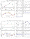 |
Fig. 1 SPIPS results for η Aql (a) and X Sgr (b) as a function of the pulsation phase. Above the figures, the p factor is indicated, along with the fitted distance d, the fitted color excess E(B − V), and the parametric CSE model. The thick gray line corresponds to the best SPIPS model, which is composed of the latter model without CSE plus an IR excess model. In the angular diameter panels, the gray curve corresponds to limb-darkened (LD) angular diameters. We provide references for the observations in Table B.2. |
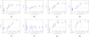 |
Fig. 2 IR excess derived by SPIPS for each star of the sample (see also Table 2): X Sgr, 7.01 d (a), U Aql, 7.02 d (b), η Aql, 7.17 d (c), β Dor, 9.84 d (d), ζ Gem, 10.15 d (e), TT Aql, 13.75 d (f), T Mon, 27.03 d (g), and U Car, 38.87 d (h). The excess is presented as the magnitude difference between the atmospheric model and the median photometric data, where positive and negative values indicate emission and absorption, respectively. The fitted IR excess (dashed green line) is modeled with a logistic function presented at the bottom of each figure. The orange bar in panel (h) for U Car corresponds to the I2 Spitzer band, ignored in the fit due to CO band-head absorption at 4.6 micron (Marengo et al. 2010a; Scowcroft et al. 2016; Gallenne et al. 2021). |
IR excess derived by SPIPS.
3.3 Angular diameter at the epoch of observations
3.3.1 Pulsation phase at the MATISSE observation epoch
In order to consistently compare MATISSE observations to the photospheric model of each star, it is necessary to derive an accurate pulsation phase corresponding to the epoch of observations. However, the pulsation periods of Cepheids are subject to a period-change effect caused by secular evolution or more erratic nonevolutionary effects (Turner et al. 2006; Csörnyei et al. 2022; Rathour et al. 2024). For X Sgr, U Aql, η Aql, and U Car, we chose a recent pulsation period and reference epoch from Gaia DR3 to mitigate the effect of a period change with respect to the time of the MATISSE observations. This was particularly useful for U Car because of its high rate of period changes (Csörnyei et al. 2022). For β Dor, ζ Gem, TT Aql, and T Mon, we adopted the SPIPS values. We summarize our choice in Table 3.
We assumed a secular period evolution for each of our stars after inspecting the O–C diagrams constructed by Csörnyei et al. (2022) and adopting their rate of period change. In the case of β Dor, the O–C diagram from Csörnyei et al. (2022) presents scattered variations, similarly to other Cepheids in the resonance region. We preferred to adopt the period-change rate derived by SPIPS. We note that only T Mon and U Car are affected by a high rate of period changes (10–100 s/yr) that can significantly affect the accuracy of the derivation of the pulsation phase at the MATISSE observation epoch. Additionally, U Car presents a clear wave-like trend in the O–C diagram, which was interpreted as a perturbation of its orbital motion by a companion.
3.4 Uniform-disk angular diameter of the star sample
Using the SPIPS model, we interpolated the limb-darkened (LD) angular diameter at the pulsation phase of each Cepheid corresponding to the MATISSE observations. The LD angular diameter is physically equivalent to the bolometric radius of the photosphere entering the Stefan-Boltzmann law. However, interferometric observations in the IR cannot resolve the LD effect of the star, but only measure the UD angular diameter. Thus, we converted the LD into the UD angular diameter in the L band following the standard procedure described, for example, by Nardetto et al. (2020), and the tables from Claret & Bloemen (2011). To this end, we used effective temperature and surface gravity interpolated by SPIPS at the specific date of the observation assuming solar metallicity and a standard microturbulent velocity of 2 km/s. We did not correct for the LD effect in the N band because its effect is negligible. Moreover, the measured visibility in the N band does not permit a comparison with the angular diameter of the star, as discussed in Sect. 6. The uncertainty of the derived angular diameter is dominated by systematic uncertainties from the SPIPS fitting and pulsation-phase estimation. For the SPIPS models that are constrained by complete datasets and a good pulsation coverage of the angular diameter (X Sgr, η Aql, β Dor, and ζ Gem), we assumed an uncertainty of 2% on the angular stellar diameter, and we assumed 4% for the other stars. We summarize our choice of the ephemerides and the derived angular diameters at the pulsation phase of the MATISSE observations in Table 3.
Cepheid ephemeris, fluxes, and angular diameters of the star sample.
4 Measured flux in the L, M, and N bands
4.1 Calibration
We calibrated the total flux of the science targets Ftot,sci using the known flux of the calibrator Ftot,cal following
![Mathematical equation: $\[F_{\text {tot}, \text {sci}}(\lambda)=\frac{I_{\text {tot}, \mathrm{sci}}(\lambda)}{I_{\text {tot}, \text {cal}}(\lambda)} \times F_{\text {tot}, \text {cal}}(\lambda),\]$](/articles/aa/full_html/2025/02/aa52827-24/aa52827-24-eq9.png) (2)
(2)
where Itot,sci and Itot,cal are the observed total raw flux of the science target and the calibrator, respectively. When available, we used SED templates of the standard stars from Cohen et al. (1999) to derive Ftot,cal (see Table 1). For the following Cepheids, we calibrated the total flux owing to accurate calibrator templates: U Aql, η Aql, ζ Gem, TT Aql, and T Mon. However, for three Cepheids (X Sgr, β Dor, and U Car), none of their calibrators have available templates. In these cases, we interpolated the SED from a grid of ATLAS9 models using the effective temperature measured by Gaia (DR3 or DR2) (Gaia Collaboration 2018) (see Table 1). We note that Casagrande & VandenBerg (2018) cautioned that the effective temperature as measured by Gaia is estimated with strong assumptions. However, in the Rayleigh-Jeans domain, the absolute flux level mostly depends on the angular stellar diameter, which is well constrained for all the calibrators. We do not expect strong biases since the effective temperature for two of these calibrators, HD 101162 and HD 59219, is consistent with the temperature obtained from UVES spectra (Alves et al. 2015). Then, we used the UD angular diameter in the N band from the JMMC catalog to rescale the theoretical SED to the specific solid angle of observation. We neglected the airmass difference since the airmass between target and calibrators is comparable to within less than 10%, except for U Car (see Table A.1). Moreover, while a chromatic correction exists for the N band (Schütz & Sterzik 2005), it is not calibrated (to our knowledge) for the L and M bands.
In the N band, the total flux of U Aql (≈1 Jy) is at the lower limit of the UT sensitivity with MATISSE for accurate visibility measurements. Instead, we used the correlated flux, which is the flux contribution from the spatially unresolved structures of the source. We calibrated the correlated flux of the science target Fcorr,sci following
![Mathematical equation: $\[F_{\text {corr,sci }}=\frac{I_{\text {corr,sci }}}{I_{\text {corr,cal }}} \times F_{\text {tot,cal }} \times V_{\text {cal}},\]$](/articles/aa/full_html/2025/02/aa52827-24/aa52827-24-eq10.png) (3)
(3)
where Icorr,sci and Icorr,cal are the observed raw correlated fluxes of the science target and the calibrator, respectively, and Vcal is the calibrator visibility. For this absolute calibration of the correlated flux, we had a robust interferometric calibrator with an atmospheric template given by Cohen et al. (1999).
The calibrated total fluxes in the L, M, and N bands are presented in Fig. 3. We discarded the spectral region between 9.3 and 10 μm because it includes a telluric ozone absorption feature around 9.6 μm that strongly impacts the data quality. We also overplot the SPIPS SED of each Cepheid at the specific phase of the MATISSE observations as derived in Sect. 3 (see the gray curves in Fig. 3).
4.2 Analysis
We drew several important preliminary conclusions. First of all, the L-,M-, and N-band fluxes are aligned with a pure Rayleigh–Jeans slope. In particular, the N-band spectra indicate the absence of oxygen-rich dust emission for all Cepheids of our sample, such as silicates, which exhibit a prominent feature between 9 and 12 micron (Draine & Lee 1984). In the case of η Aql, ζ Gem, and ℓ Car, Spitzer low-resolution spectra already revealed the absence of dust emission (Hocdé et al. 2020b, 2021). Interestingly, Gallenne et al. (2013) suggested silicate dust features based on MIDI/VLTI observations for X Sgr and T Mon, while our observations yield the opposite result for these two stars, as we do not observe any peculiar trends in the N-band flux. We discuss this difference further in the analysis of the MATISSE visibility in Sect. 6.
Second, the SEDs as derived by SPIPS at the specific phase of MATISSE observations agree with the calibrated flux within the uncertainties, except for β Dor, for which we derive an excess up to about 50% of the MATISSE flux in L, M, and N bands. We did not find the origin of this discrepancy since the photometric bands from SPIPS are well adjusted, and on the other hand, the calibration seems reliable with good observing conditions, similar airmass, and a consistent template of the calibrator HD 59219. However, it is not relevant to derive the IR excess from a MATISSE flux observation that could be due to CSEs because the measurements have rather large uncertainties (≥10%≈0.10 mag), which is not suited for deriving subtle IR excesses of about 5% of the total flux.
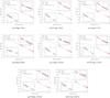 |
Fig. 3 MATISSE calibrated flux in the L, M, and N bands together with the ATLAS9 atmospheric model interpolated for each star by SPIPS at the specific pulsation phase of observations. The blue bars represent the photometry interpolated at the phase of the MATISSE observations by SPIPS. In the case of U Aql, the N-band flux is the correlated flux. See Sect. 4 for details of the calibration. |
5 Closure phase
MATISSE also provides closure phase measurements, which contain information about the spatial centro-(a)symmetry of the brightness distribution of the source. Given the phase measurements of a telescope triplet i jk, the closure phase is the combination ϕi jk = ϕij + ϕjk − ϕik. One of the advantages of the closure equation is that it cancels out any atmospheric or baseline-dependent phase error (Jennison 1958). For all the closure phase measurements, we find an average of about 0° in the L, M and the N bands (see Figs. C.1 and C.2). In N band, the spectral window beyond 10 μm is too noisy to obtain meaningful conclusion for U Aql, TT Aql and T Mon. Overall, down to a sub-degree level, our closure phase measurements are consistent with the absence of significant brightness spatial asymmetries in the environment for all Cepheids in L, M and N bands.
6 Visibility in L, M and N bands
6.1 Calibration
As discussed in Sect. 2.2 the targets were calibrated using specific calibrators for the L, M band, and the N bands. Hence, we performed by default a CAL-SCI sequence of calibration separately for both L and N-bands. In some cases, we obtained a better calibration in the L band using the brighter N-band calibrator instead, as it is the case for example of η Aql. For X Sgr, β Dor and ζ Gem we could only observe one calibrator. In this case the same calibrator was used for the calibration in L and N-bands. Moreover, each target required a special attention because of peculiar atmospheric conditions or technical problems during the observations that could affect the visibility curves. Hence, we scrutinized the raw visibilities to ensure their overall quality for both target and calibrators. When we observed an obvious discrepant exposure for a corresponding baseline – generally deviating by more than 2σ compared to other exposures of adjacent baselines – we simply excluded this latter from the analysis. For U Aql we note that the calibrated visibilities are slightly above 1. The results of the calibration for the squared visibility V2 in L and M bands and the visibility V in the N band are presented in Figs. 4 and 5 respectively; the error bars represent the standard deviation between the visibilities of the different exposures, within one observing sequence. The visibility curve associated with the expected UD angular diameter of the star as derived from the SPIPS analysis is shown for comparison (see orange curves in Figs. 4 and 5). We also displayed the visibility of the latter model taking into account the CSE model derived by SPIPS in each case (see dashed curves in Figs. 4 and 5).
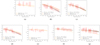 |
Fig. 4 MATISSE-calibrated squared visibilities in the L and M bands: U Aql, 7.02 d (a), η Aql, 7.17 d (b), β Dor, 9.84 d (c), ζ Gem, 10.15 d (d), TT Aql, 13.75 d (e), T Mon, 27.03 d (f), and U Car, 38.87 d (g). The thick orange curve is the visibility derived from the UD diameter of the star by SPIPS at the specific phase of the MATISSE observation. The dashed orange line represents the visibility derived for the star plus the CSE model by SPIPS (see Sect. 3.2). The dashed black curve is the fit of the UD angular diameter with the error derived from the bootstrap method (see Table 4). No model adjustments (labeled FIT) are presented for U Aql and TT Aql because these stars are mostly unresolved and are more affected by uncertainties in the absolute visibility scale. X Sgr data are impacted by a too short coherence time and thus are not presented. |
6.2 Results in the L and M-bands
For all Cepheids of our sample, the MATISSE observations in the L and M bands are in agreement with the SPIPS UD angular diameter. Moreover, we derived the UD angular diameter from the MATISSE observations in L and M bands by fitting the squared visibility ![Mathematical equation: $\[V_{\mathrm{UD}}^{2}(f)\]$](/articles/aa/full_html/2025/02/aa52827-24/aa52827-24-eq11.png) following:
following:
![Mathematical equation: $\[V_{\mathrm{UD}}^{2}(f)=\left(2 \frac{J_{1}\left(\pi \theta_{\mathrm{UD}} f\right)}{\pi \theta_{\mathrm{UD}} f}\right)^{2},\]$](/articles/aa/full_html/2025/02/aa52827-24/aa52827-24-eq12.png) (4)
(4)
where J1 is the Bessel function of the first order and where f=Bp/λ is the spatial frequency (Bp the length of the projected baseline). We used the PMOIRED4 code (Mérand 2022) to perform the fit of the UD angular diameter and estimate the uncertainties via the bootstrap method. We provide the UD angular diameters in Table 4. From these results it is not possible to resolve a CSE emission of the order of 0.05–0.10 mag in the L-band. As we can see from Fig. 4, the SPIPS CSE model (dashed line) cannot be resolved by MATISSE. We provide upper limits for both the size and the CSE flux contribution in Sect. 6.4.
Fits of UD angular diameter.
6.3 Results in the N-band
In the N-band, the visibilities are more affected by the thermal background which impact the absolute visibility level and the signal to noise ratio. However, it is clear from the Fig. 5 that we do not resolve any environment for the six stars presented since we obtain rather horizontal visibility level without any significant trend. This observation motivates us to perform a weighted mean of the visibility at different baseline which highlight the horizontal visibility trend (see black curve in Fig. 5). This result is in agreement with the SED in the N-band presented in Sect. 4 which does not present silicate emission features which should produce a large dip of the visibility centered on 9.7 μm. As for the SED analysis, the measured visibilities with MATISSE indicates that there is not resolved CSE around T Mon which disagrees with the results found by Gallenne et al. (2013) with MIDI/VLTI (see Fig. A.1e). This discrepancy cannot be attributed to a difference of calibrator, as we chose the same calibrator as in G13, namely 30 Gem and 18 Mon. We note that Groenewegen (2020) also found contradictory results with the G13 SED of T Mon. However, G13 reported that the excess of T Mon might suffer from sky background contamination which might be at the origin of this difference. In the case of X Sgr, the MATISSE N-band visibility is also strongly affected by the poor atmospheric conditions and is not discussed. Thus, we cannot compare with the results from G13 who resolved a CSE in the N-band with MIDI/VLTI with a relative CSE contribution of f = 13.3 ± 0.7%. However, the total flux of X Sgr in the N-band as measured by MATISSE suggests that there is an absence of silicate features (see Figs. 3a). This result disagrees with the observations from Gallenne et al. (2012, 2013) who detected a trend in the SED, modeled with a radiative transfer of CSE with dust mixture.
In the case of U Car, Gallenne et al. (2012) detected a spatially extended emission with a significant residual flux of ΔF = 16.3 ± 1.4% in the N-band. They also proposed a model of silicate dust mixture to explain the SED. While the IR excess in the N-band as derived by SPIPS is in close agreement with Δmag= 0.13 mag (see Fig. 2h and Table 2), we do not find silicate feature in the MATISSE N-band spectrum and visibility, which suggest another physical source of the IR emission. Gallenne et al. (2012) note however that their observations could be affected by the interstellar-cirrus background emission in the region of this star also observed from IRAC 8 μm observations (Barmby et al. 2011).
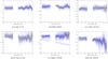 |
Fig. 5 Visibility in the N band plotted against the wavelength. The black curve represents the weighted mean of the observations. U Aql is not presented since we only measured the correlated flux and the X Sgr photometry in the N band was not usable. The spectral band between 9.3 and 10 micron was removed because the atmosphere is not transmissive. In the case of T Mon, we overplot the weighted mean of MIDI/VLTI observation as given by Gallenne et al. (2013) for comparison. |
6.4 Upper limits on the CSE in the L and M bands
Our results in L, M and N bands suggest that we do not resolve any significant circumstellar emission for all the stars of our sample. However, the large error bars prevent the detection of a compact and/or small emission around these stars. For example, the SPIPS CSE model is also consistent with the MATISSE visibilities (see the dashed orange lines in Fig. 4). To better illustrate the difficulty of resolving compact CSE on the L-band visibility curve, we present different CSE models in Fig. 6. The shape of the first visibility lobe provides crucial information regarding the size and flux of the CSE. However, it is difficult to consistently define upper limits for each star as the flux and size of the CSE are fully degenerate within the uncertainty. In order to provide upper limits to the extension and emission of the CSE, we applied a geometrical model on the measured L and M-band visibilities. Each Cepheid was modeled with a UD angular diameter θUD that was fixed to the one at the specific phase of the observation derived by SPIPS in the L band from Table 3. The visibility VUD(f) was derived according to Eq. (4) presented in Sect. 6.2. We superimposed a CSE modeled with a Gaussian intensity distribution with a full-width at half maximum (FWHM) θCSE on this star model. The visibility of the envelope VCSE(f) was derived following the Van Cittert-Zernicke theorem (Berger & Segransan 2007),
![Mathematical equation: $\[V_{\mathrm{CSE}}(f)=\exp \left[-\frac{\left(\pi \theta_{\mathrm{CSE}} f\right)^{2}}{4 {\ln} 2}\right].\]$](/articles/aa/full_html/2025/02/aa52827-24/aa52827-24-eq13.png) (5)
(5)
We note that other models were used for the CSE of Cepheids, such as a shell or optically thin envelope (Mérand et al. 2006; Gallenne et al. 2012). The choice of a Gaussian intensity distribution for the envelope was used for simplicity because we currently lack physical justifications. This model is consistent with the centro-symmetric structure given by a zero closurephase in Sect. 5, however. Thus, we computed the total squared visibility of the star plus CSE model,
![Mathematical equation: $\[V_{\mathrm{tot}}^{2}(f)=\left(\left|F_{\star} ~V_{\mathrm{UD}}(f)+F_{\mathrm{CSE}} ~V_{\mathrm{CSE}}(f)\right|\right)^{2},\]$](/articles/aa/full_html/2025/02/aa52827-24/aa52827-24-eq14.png) (6)
(6)
where F⋆ and FCSE are the normalized stellar and CSE flux contribution to the total flux, respectively, normalized to unity F⋆ + FCSE = 1. In this process, we computed ![Mathematical equation: $\[V_{\text {tot}}^{2}(f)\]$](/articles/aa/full_html/2025/02/aa52827-24/aa52827-24-eq15.png) for all combinations of the CSE flux contribution and size. We then derived the reduced χ2 map by comparing it with the MATISSE visibilities (see Fig. 7).
for all combinations of the CSE flux contribution and size. We then derived the reduced χ2 map by comparing it with the MATISSE visibilities (see Fig. 7).
As shown by the χ2 map for all stars of our sample, the flux contribution from these observations cannot be constrained for a compact envelope below 3–4 R⋆. Conversely, a faint circumstellar emission is also consistent for different CSE sizes. In order to provide quantitative limits on the CSE characteristics, we calculated the residuals between the observations and models. We excluded models with residuals above 2 σ. We provide the upper limits of the CSE flux contribution for different CSE radius in Table 5, which is also vizualized in Fig. 7. These upper limits are overall similar for all stars. In particular, we can securely rule out envelopes that are simultaneously large and bright (R>10 R⋆;f > 10%) for the entire star sample.
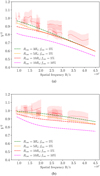 |
Fig. 6 Examples of CSE models with a Gaussian brightness intensity distribution in the case of (a) β Dor (1.86 mas) and (b) U Car (0.80 mas). The examples illustrate the difficulty of resolving a compact CSE with MATISSE/VLTI. For a CSE flux contribution of 5% of the total flux, compact CSEs between 5 and 10 R⋆ cannot be resolved (see the green, orange, and red models). The large and bright model shown as the dashed magenta line is excluded in both stars, however. The upper limits for different CSE models are given in Table 5. |
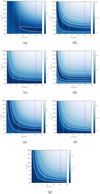 |
Fig. 7 Reduced χ2 map as a function of the flux contribution fCSE and FWHM (RCSE) of the Gaussian CSE model in the L and M bands: U Aql, 7.02 d (a), η Aql, 7.17 d (b), β Dor, 9.84 d (c), ζ Gem, 10.15 d (d), TT Aql, 13.75 d (e), T Mon, 27.03 d (f), and U Car, 38.87 d (g). The dashed cyan, orange, and purple lines represent different CSE radii (FWHM) for which we provide the upper limit on the CSE flux contribution. It is displayed as a square (see Table 5). The weak flux contribution (<5%) does not permit us to constrain the CSE dimensions. Conversely, the flux of the compact envelope (<3–4 R⋆) cannot be determined. Large and bright models (R>10 R⋆f > 10%, purple squares) can be excluded, however. |
6.5 Radiative transfer models of dusty CSE
The IR excess and the N-band observations allow us to constrain the CSE models based on the dust grains. To this end, we computed dusty CSE models with the radiative transfer code DUSTY (Ivezic et al. 1999) in order to show the theoretical visibility and IR excess in these cases. While it is possible to fit CSE models by fine-tuning the dust composition and other characteristics, we opted for a simpler approach and selected representative test cases to illustrate these models. We chose η Aql and T Mon as test cases. These stars have different angular diameters (≈1.8 and 0.8 mas, respectively). For each star, we modeled a blackbody as the central source by adopting the stellar luminosity, temperature, and radius from SPIPS at the phase corresponding to the MATISSE observations. To explore the characteristic mineralogy of oxygen-rich stars, we modeled three types of the dust composition: iron, silicates, and alumina. We used optical constants from Henning & Stognienko (1996), Ossenkopf et al. (1992), and Begemann et al. (1997) respectively. For each model, the condensation temperature was arbitrarily fixed at 1200 K, which is slightly higher than in the condensation models from Gail & Sedlmayr (1999) at relatively low gas pressure. A standard grain size distribution (Mathis et al. 1977) and dust density (nd ∝ r−2) were used, while the optical depth was varied for each dust type. From these models, we computed the N-band visibility for a baseline of 130 m, which matches the maximum VLTI baseline, and we derived the corresponding IR excess for comparison with SPIPS results. The results are presented in Figs. 8 and A.1.
These results allowed us to constrain the optical depth for each dust type. We find that for both η Aql and T Mon, an optical depth of about τv = 0.001 or lower aligns well with MATISSE observations. This indicates that if dust exists around Cepheids, it is likely too faint to be resolved. However, CSEs with optical depths of at least τV = 0.01 would be clearly resolved for every dust type. For comparison, Gallenne et al. (2013) fit τV = 0.151 ± 0.042 to explain the MIDI/VLTI visibility of T Mon, with an iron content of 80%. This content is excluded from our observations in Fig. A.1. On the other hand, Gallenne et al. (2013) derived τV = 0.008 ± 0.002 for X Sgr, with a visibility range of 0.9–1.0 measured by MIDI/VLTI. Given the relatively small angular diameter of X Sgr (≈1.35 mas), we do not expect to resolve an envelope this faint with MATISSE. Our simple tests also agree with the results of Groenewegen (2020), who fit the IR excess of Galactic Cepheids with iron as the main dust component. The optical depth ranged from about 10−4 to 10−3. In particular, the optical depth derived by Groenewegen (2020) in the case of the CSE of η Aql and ζ Gem (with an iron content above 90%) would yield a visibility of V ≈ 0.95, which would agree with our MATISSE observations. Figs. 8 and A.1 show that silicate and alumina predominantly emit in the N band, and a level of ≈ 0.10 mag in the N band gives no IR excess in the K and L bands. The only exception is the iron component, which is able to produce noticeable near-IR emission. For η Aql and T Mon, an iron optical depth of τV = 0.01 would result in IR excess that closely matches the SPIPS estimates, with corresponding values of ΔK = 0.02 mag, ΔL = 0.05 mag, and ΔN = 0.13 mag for η Aql, and ΔK = 0.03 mag, ΔL = 0.07 mag, and ΔN = 0.15 mag for T Mon. However, we consider it unlikely that almost nothing but iron alone would form in these environment. As discussed in the introduction, a compact envelope of about 2–4 R⋆ might be too hot for dust condensation. A more plausible explanation for the observed near-IR excess is a compact, ionized gas envelope that behaves similarly to a chromosphere and emits continuous free-free emission (Hocdé et al. 2020b).
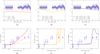 |
Fig. 8 Visibility in the N band and IR excess from CSE models of dust computed with DUSTY for the Cepheid η Aql. From left to right, the three cases correspond to iron, silicates, and aluminum oxide, which are plotted in red, yellow, and purple, respectively. For each CSE model, we used a different optical depth, as indicated in the legend. |
Upper limit at 2σ for the flux of the CSE.
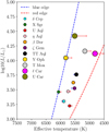 |
Fig. 9 Cepheid sample observed with MATISSE/VLTI (This work, and Hocdé et al. 2021) completed with δ Cep and Y Oph observed with CHARA (Mérand et al. 2006, 2007; Nardetto et al. 2016). The mean luminosity and effective temperature in the instability strip are derived by SPIPS. Blueward or redward crossings are indicated by arrows depending on the sign of the period change. The dotted black circles indicate stars whose CSEs are thought to be resolved by interferometry based on previous studies. The dotted red circle represents a star with a confirmed CSE around ℓ Car. |
7 Conclusion
We explored the circumstellar emission for a group of Cepheids with a pulsation period of 7 up to about 40 days that are distributed at different locations within the instability strip, as shown in Fig. 9. From the results of MATISSE observations alone, we showed that the closure phases for all Cepheids are consistent with a central symmetry in the L, M, and N bands. We also found the absence of dust emission for a relatively large set of Cepheids with different pulsation periods and stellar parameters. It is not excluded that a circumstellar dust envelope can form for Cepheids with longer pulsation periods, however (see, for example, Kovtyukh et al. 2024). In this context, it is important to enlarge the sample of Cepheids with interferometric observations in the N band to definitely conclude on the absence of dusty envelopes. However, an important caveat is that the current MATISSE observations cannot effectively constrain the size of the CSE, especially when its flux contribution is weak (around 5%). While a CSE that is simultaneously bright (≈10%) and large (≈10 R⋆) can be ruled out, the observations are compatible with the presence of a compact CSE within the uncertainties, as modeled in previous studies. We note that our analysis was based on a single snapshot for each star, and these observations are therefore exposed to calibration bias. However, the homogeneity of these results, which are based on eight different Cepheids, provides a robust picture of the CSE model across the instability strip.
On the other hand, interferometric detections of CSEs are biased toward larger angular diameters, such as that of ℓ Car. It is therefore not possible to definitely conclude on the characteristics of the envelope through the instability strip with MATISSE/VLTI. Because only a few observations have been made so far, it is also difficult to observe any relation, as shown in Fig. 9, that would depend on the evolutionary stage of the star. Based on the resolved CSE emission, ℓ Car is likely the most significant example because it was observed with MIDI, VISIR, and MATISSE. All other CSEs that were resolved up to now, such as those around δ Cep, Y Oph, and Polaris, must be confirmed with additional observations from the northern hemisphere.
In future studies, follow-up observations using GRAV4MAT with a higher angular resolution could significantly reduce the errors and provide more precise constraints, especially for bright targets in the mid-IR. On the other hand, observations at a higher spatial frequency in the near-IR are necessary to resolve the circumstellar emission of stars with a smaller angular diameter. Further observations of Cepheids using GRAVITY/VLTI in K band (GRAVITY Collaboration 2017) and CHARA/SPICA in the visible domain (Mourard et al. 2022) will also be essential to separate the contributions of the star and the CSE.
Data availability
MATISSE reduced data are made available at ESO science archive facility. Appendix B figures are available at Zenodo: https://zenodo.org/records/14505155.
Acknowledgements
We thank the referee for the careful reading which helped to improve the paper. The research leading to these results has received funding from the European Research Council (ERC) under the European Union’s Horizon 2020 research and innovation programme (grant agreements No. 695099 and No. 951549). This work received the funding from the Polish-French Marie Skłodowska-Curie and Pierre Curie Science Prize awarded by the Foundation for Polish Science. This work also received funding from the Polish Ministry of Science and Higher Education grant agreement 2024/WK/02. The authors acknowledge the support of the French Agence Nationale de la Recherche (ANR) under grant ANR-23-CE31-0009-01 (Unlock-pfactor). RS is supported by the National Science Center, Poland, Sonata BIS project 2018/30/E/ST9/00598. This research made use of the SIMBAD and VIZIER (http://cdsarc.u-strasbg.fr/) databases at CDS, Strasbourg (France) and the electronic bibliography maintained by the NASA/ADS system. Based on observations made with ESO telescopes at Paranal observatory under program IDs: 104.D-0554(B), 106.21RL.001, 106.21RL. 002 and 106.21RL.003. This research has benefited from the help of SUV, the VLTI user support service of the Jean-Marie Mariotti Center (http://www.jmmc.fr/suv.htm). This research has also made use of the Jean-Marie Mariotti Center Aspro service http://www.jmmc.fr/aspro. This research also made use of Astropy, a community-developed corePython package for Astronomy (Astropy Collaboration 2018).
Appendix A Additional material
Journal of the observations.
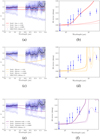 |
Fig. A.1 Same as Fig. 8 but in the case of T Mon. Optical depth of dust are given for τV = 0.01, 0.001 and 0.0005. |
Appendix B SPIPS dataset and fitted pulsational model of the star sample
Comparison of effective temperature, color excess and LD angular diameter from SPIPS by Trahin et al. (2021) and Gallenne et al. (2021).
References of observations used for the SPIPS fitting.
Appendix C Closure phase observations
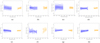 |
Fig. C.1 Closure phase in L and M bands for each triplet combination: X Sgr (a), U Aql (b), η Aql (c), β Dor (d), ζ Gem (e), TT Aql (f), T Mon (g), and U Car (h). |
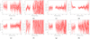 |
Fig. C.2 Closure phase in N band for each triplet combination: X Sgr (a), U Aql (b), η Aql (c), β Dor (d), ζ Gem (e), TT Aql (f), T Mon, N (g), and U Car, N (h). |
References
- Allouche, F., Robbe-Dubois, S., Lagarde, S., et al. 2016, SPIE Conf. Ser., 9907, 99070C [NASA ADS] [Google Scholar]
- Alves, S., Benamati, L., Santos, N. C., et al. 2015, MNRAS, 448, 2749 [Google Scholar]
- Ammons, S. M., Robinson, S. E., Strader, J., et al. 2006, ApJ, 638, 1004 [NASA ADS] [CrossRef] [Google Scholar]
- Anderson, R. I. 2024, arXiv e-prints [arXiv:2403.02801] [Google Scholar]
- Anderson, R. I., Mérand, A., Kervella, P., et al. 2016, MNRAS, 455, 4231 [Google Scholar]
- Anderson, R. I., Viviani, G., Shetye, S. S., et al. 2024, A&A, 686, A177 [NASA ADS] [CrossRef] [EDP Sciences] [Google Scholar]
- Astropy Collaboration (Price-Whelan, A. M., et al.) 2018, AJ, 156, 123 [Google Scholar]
- Baade, W. 1926, Astron. Nachr., 228, 359 [NASA ADS] [CrossRef] [Google Scholar]
- Barmby, P., Marengo, M., Evans, N. R., et al. 2011, AJ, 141, 42 [NASA ADS] [CrossRef] [Google Scholar]
- Barnes, III, T. G., Fernley, J. A., Frueh, M. L., et al. 1997, PASP, 109, 645 [NASA ADS] [CrossRef] [Google Scholar]
- Barnes, III, T. G., Storm, J., Jefferys, W. H., Gieren, W. P., & Fouqué, P. 2005, ApJ, 631, 572 [NASA ADS] [CrossRef] [Google Scholar]
- Begemann, B., Dorschner, J., Henning, T., et al. 1997, ApJ, 476, 199 [NASA ADS] [CrossRef] [Google Scholar]
- Berdnikov, L. N. 2008, VizieR Online Data Catalog: II/285 [NASA ADS] [Google Scholar]
- Berdnikov, L. N., & Turner, D. G. 2002, VizieR Online Data Catalog: J/ApJS/137/209 [NASA ADS] [Google Scholar]
- Berdnikov, L., Mattei, J. A., & Beck, S. J. 2003, jaavso, 31, 146 [NASA ADS] [Google Scholar]
- Berger, J. P., & Segransan, D. 2007, New A Rev., 51, 576 [NASA ADS] [CrossRef] [Google Scholar]
- Bono, G., Caputo, F., & Castellani, V. 2006, Mem. Soc. Astron. Italiana, 77, 207 [NASA ADS] [Google Scholar]
- Borgniet, S., Kervella, P., Nardetto, N., et al. 2019, A&A, 631, A37 [NASA ADS] [CrossRef] [EDP Sciences] [Google Scholar]
- Bourgés, L., Lafrasse, S., Mella, G., et al. 2014, in Astronomical Society of the Pacific Conference Series, 485, Astronomical Data Analysis Software and Systems XXIII, eds. N. Manset, & P. Forshay, 223 [Google Scholar]
- Bras, G., Kervella, P., Trahin, B., et al. 2024, A&A, 684, A126 [NASA ADS] [CrossRef] [EDP Sciences] [Google Scholar]
- Breitfelder, J., Mérand, A., Kervella, P., et al. 2016, A&A, 587, A117 [CrossRef] [EDP Sciences] [Google Scholar]
- Caputo, F., Bono, G., Fiorentino, G., Marconi, M., & Musella, I. 2005, ApJ, 629, 1021 [CrossRef] [Google Scholar]
- Casagrande, L., & VandenBerg, D. A. 2018, MNRAS, 479, L102 [NASA ADS] [CrossRef] [Google Scholar]
- Castelli, F., & Kurucz, R. L. 2003, in IAU Symposium, 210, Modelling of Stellar Atmospheres, eds. N. Piskunov, W. W. Weiss, & D. F. Gray, A20 [Google Scholar]
- Chelli, A., Duvert, G., Bourgès, L., et al. 2016, A&A, 589, A112 [NASA ADS] [CrossRef] [EDP Sciences] [Google Scholar]
- Claret, A., & Bloemen, S. 2011, A&A, 529, A75 [NASA ADS] [CrossRef] [EDP Sciences] [Google Scholar]
- Cohen, M., Walker, R. G., Carter, B., et al. 1999, AJ, 117, 1864 [Google Scholar]
- Coulson, I. M., & Caldwell, J. A. R. 1985, South Afr. Astron. Observ. Circ., 9, 5 [Google Scholar]
- Cruzalèbes, P., Petrov, R. G., Robbe-Dubois, S., et al. 2019, MNRAS, 490, 3158 [Google Scholar]
- Csörnyei, G., Szabados, L., Molnár, L., et al. 2022, MNRAS, 511, 2125 [CrossRef] [Google Scholar]
- Davis, J., Ireland, M. J., Jacob, A. P., et al. 2008, in The Power of Optical/IR Interferometry: Recent Scientific Results and 2nd Generation, eds. A. Richichi, F. Delplancke, F. Paresce, & A. Chelli, 105 [CrossRef] [Google Scholar]
- Deasy, H. P. 1988, MNRAS, 231, 673 [NASA ADS] [Google Scholar]
- Deasy, H., & Butler, C. J. 1986, Nature, 320, 726 [CrossRef] [Google Scholar]
- Draine, B. T., & Lee, H. M. 1984, ApJ, 285, 89 [NASA ADS] [CrossRef] [Google Scholar]
- Eaton, J. A. 2020, jaavso, 48, 91 [NASA ADS] [Google Scholar]
- ESA 1997, ESA Special Publication, 1200, The HIPPARCOS and TYCHO catalogues. Astrometric and photometric star catalogues derived from the ESA HIPPARCOS Space Astrometry Mission [Google Scholar]
- Feast, M. W. 2008, MNRAS, 387, L33 [NASA ADS] [CrossRef] [Google Scholar]
- Fokin, A. B., Gillet, D., & Breitfellner, M. G. 1996, A&A, 307, 503 [NASA ADS] [Google Scholar]
- Fraschetti, F., Anastasopoulou, K., Drake, J. J., & Evans, N. R. 2023, ApJ, 944, 62 [NASA ADS] [CrossRef] [Google Scholar]
- Freedman, W. L., & Madore, B. F. 2024, in IAU Symposium, 376, IAU Symposium, eds. R. de Grijs, P. A. Whitelock, & M. Catelan, 1 [Google Scholar]
- Gaia Collaboration 2022, VizieR Online Data Catalog: I/355 [Google Scholar]
- Gaia Collaboration (Prusti, T., et al.) 2016, A&A, 595, A1 [NASA ADS] [CrossRef] [EDP Sciences] [Google Scholar]
- Gaia Collaboration (Brown, A. G. A., et al.) 2018, A&A, 616, A1 [NASA ADS] [CrossRef] [EDP Sciences] [Google Scholar]
- Gail, H.-P., & Sedlmayr, E. 1999, A&A, 347, 594 [Google Scholar]
- Gallenne, A., Kervella, P., & Mérand, A. 2012, A&A, 538, A24 [NASA ADS] [CrossRef] [EDP Sciences] [Google Scholar]
- Gallenne, A., Mérand, A., Kervella, P., et al. 2013, A&A, 558, A140 [NASA ADS] [CrossRef] [EDP Sciences] [Google Scholar]
- Gallenne, A., Kervella, P., Mérand, A., et al. 2017, A&A, 608, A18 [NASA ADS] [CrossRef] [EDP Sciences] [Google Scholar]
- Gallenne, A., Kervella, P., Evans, N. R., et al. 2018, ApJ, 867, 121 [Google Scholar]
- Gallenne, A., Kervella, P., Borgniet, S., et al. 2019, A&A, 622, A164 [NASA ADS] [CrossRef] [EDP Sciences] [Google Scholar]
- Gallenne, A., Mérand, A., Kervella, P., et al. 2021, A&A, 651, A113 [NASA ADS] [CrossRef] [EDP Sciences] [Google Scholar]
- GRAVITY Collaboration (Abuter, R., et al.) 2017, A&A, 602, A94 [NASA ADS] [CrossRef] [EDP Sciences] [Google Scholar]
- Groenewegen, M. A. T. 2020, A&A, 635, A33 [EDP Sciences] [Google Scholar]
- Groenewegen, M. A. T., & Lub, J. 2023, A&A, 676, A136 [NASA ADS] [CrossRef] [EDP Sciences] [Google Scholar]
- Henning, T., & Stognienko, R. 1996, A&A, 311, 291 [NASA ADS] [Google Scholar]
- Hocdé, V., Nardetto, N., Borgniet, S., et al. 2020a, A&A, 641, A74 [EDP Sciences] [Google Scholar]
- Hocdé, V., Nardetto, N., Lagadec, E., et al. 2020b, A&A, 633, A47 [NASA ADS] [CrossRef] [EDP Sciences] [Google Scholar]
- Hocdé, V., Nardetto, N., Matter, A., et al. 2021, A&A, 651, A92 [NASA ADS] [CrossRef] [EDP Sciences] [Google Scholar]
- Hocdé, V., Moskalik, P., Gorynya, N. A., et al. 2024a, A&A, 689, A224 [NASA ADS] [CrossRef] [EDP Sciences] [Google Scholar]
- Hocdé, V., Smolec, R., Moskalik, P., Singh Rathour, R., & Ziółkowska, O. 2024b, A&A, 683, A233 [NASA ADS] [CrossRef] [EDP Sciences] [Google Scholar]
- Hubble, E. P. 1925, ApJ, 62, 409 [NASA ADS] [CrossRef] [Google Scholar]
- Hubble, E. P. 1926, ApJ, 63, 236 [NASA ADS] [CrossRef] [Google Scholar]
- Hubble, E. 1929a, PNAS, 15, 168 [CrossRef] [Google Scholar]
- Hubble, E. P. 1929b, ApJ, 69, 103 [NASA ADS] [CrossRef] [Google Scholar]
- Ivezic, Z., Nenkova, M., & Elitzur, M. 1999, DUSTY: Radiation transport in a dusty environment, Astrophysics Source Code Library [record ascl:9911.001] [Google Scholar]
- Jennison, R. C. 1958, MNRAS, 118, 276 [Google Scholar]
- Keller, S. C. 2008, ApJ, 677, 483 [NASA ADS] [CrossRef] [Google Scholar]
- Kervella, P., Nardetto, N., Bersier, D., Mourard, D., & Coudé du Foresto, V. 2004, A&A, 416, 941 [NASA ADS] [CrossRef] [EDP Sciences] [Google Scholar]
- Kervella, P., Mérand, A., Perrin, G., & Coudé du Foresto, V. 2006, A&A, 448, 623 [NASA ADS] [CrossRef] [EDP Sciences] [Google Scholar]
- Kervella, P., Mérand, A., & Gallenne, A. 2009, A&A, 498, 425 [NASA ADS] [CrossRef] [EDP Sciences] [Google Scholar]
- Kiss, L. L. 1998, in Astronomical Society of the Pacific Conference Series, 135, A Half Century of Stellar Pulsation Interpretation, eds. P. A. Bradley, & J. A. Guzik, 173 [Google Scholar]
- Kovtyukh, V. V., Andrievsky, S. M., Belik, S. I., & Luck, R. E. 2005, AJ, 129, 433 [Google Scholar]
- Kovtyukh, V. V., Chekhonadskikh, F. A., Luck, R. E., et al. 2010, MNRAS, 408, 1568 [NASA ADS] [CrossRef] [Google Scholar]
- Kovtyukh, V. V., Andrievsky, S. M., Werner, K., Korotin, S. A., & Kniazev, A. Y. 2024, A&A, 684, A145 [NASA ADS] [CrossRef] [EDP Sciences] [Google Scholar]
- Lane, B. F., Creech-Eakman, M. J., & Nordgren, T. E. 2002, ApJ, 573, 330 [NASA ADS] [CrossRef] [Google Scholar]
- Laney, C. D., & Stobie, R. S. 1992, A&AS, 93, 93 [NASA ADS] [Google Scholar]
- Leavitt, H. S. 1908, Ann. Harvard Coll. Observ., 60, 87 [NASA ADS] [Google Scholar]
- Leavitt, H. S., & Pickering, E. C. 1912, Harvard Coll. Observ. Circ., 173, 1 [Google Scholar]
- Lemaître, G. 1927, Ann. Soc. Sci. Bruxelles, 47, 49 [Google Scholar]
- Lindegren, L., Klioner, S. A., Hernández, J., et al. 2021, A&A, 649, A2 [EDP Sciences] [Google Scholar]
- Lopez, B., Lagarde, S., Jaffe, W., et al. 2014, The Messenger, 157, 5 [NASA ADS] [Google Scholar]
- Lopez, B., Lagarde, S., Petrov, R. G., et al. 2022, A&A, 659, A192 [NASA ADS] [CrossRef] [EDP Sciences] [Google Scholar]
- Luck, R. E. 2018, AJ, 156, 171 [Google Scholar]
- Luck, R. E., & Andrievsky, S. M. 2004, AJ, 128, 343 [Google Scholar]
- Madore, B. F. 1975, ApJS, 29, 219 [Google Scholar]
- Marengo, M., Evans, N. R., Barmby, P., et al. 2010a, ApJ, 709, 120 [NASA ADS] [CrossRef] [Google Scholar]
- Marengo, M., Evans, N. R., Barmby, P., et al. 2010b, ApJ, 725, 2392 [NASA ADS] [CrossRef] [Google Scholar]
- Mathis, J. S., Rumpl, W., & Nordsieck, K. H. 1977, ApJ, 217, 425 [Google Scholar]
- Matthews, L. D., Marengo, M., Evans, N. R., & Bono, G. 2012, ApJ, 744, 53 [NASA ADS] [CrossRef] [Google Scholar]
- Matthews, L. D., Marengo, M., & Evans, N. R. 2016, AJ, 152, 200 [NASA ADS] [CrossRef] [Google Scholar]
- McAlary, C. W., & Welch, D. L. 1986, AJ, 91, 1209 [NASA ADS] [CrossRef] [Google Scholar]
- Mérand, A. 2022, SPIE Conf. Ser., 12183, 121831N [Google Scholar]
- Mérand, A., Kervella, P., Coudé du Foresto, V., et al. 2006, A&A, 453, 155 [CrossRef] [EDP Sciences] [Google Scholar]
- Mérand, A., Aufdenberg, J. P., Kervella, P., et al. 2007, ApJ, 664, 1093 [Google Scholar]
- Mérand, A., Kervella, P., Breitfelder, J., et al. 2015, A&A, 584, A80 [NASA ADS] [CrossRef] [EDP Sciences] [Google Scholar]
- Millour, F., Berio, P., Heininger, M., et al. 2016, SPIE Conf. Ser., 9907, 990723 [NASA ADS] [Google Scholar]
- Moffett, T. J., & Barnes, III, T. G. 1984, ApJS, 55, 389 [NASA ADS] [CrossRef] [Google Scholar]
- Monson, A. J., & Pierce, M. J. 2011, ApJS, 193, 12 [Google Scholar]
- Monson, A. J., Freedman, W. L., Madore, B. F., et al. 2012, ApJ, 759, 146 [Google Scholar]
- Moschou, S.-P., Vlahakis, N., Drake, J. J., et al. 2020, ApJ, 900, 157 [NASA ADS] [CrossRef] [Google Scholar]
- Mourard, D., Berio, P., Pannetier, C., et al. 2022, SPIE Conf. Ser., 12183, 1218308 [NASA ADS] [Google Scholar]
- Nardetto, N., Mérand, A., Mourard, D., et al. 2016, A&A, 593, A45 [CrossRef] [EDP Sciences] [Google Scholar]
- Nardetto, N., Salsi, A., Mourard, D., et al. 2020, A&A, 639, A67 [NASA ADS] [CrossRef] [EDP Sciences] [Google Scholar]
- Nardetto, N., Gieren, W., Storm, J., et al. 2023, A&A, 671, A14 [NASA ADS] [CrossRef] [EDP Sciences] [Google Scholar]
- Neilson, H. R., & Lester, J. B. 2008, ApJ, 684, 569 [NASA ADS] [CrossRef] [Google Scholar]
- Neilson, H. R., Ngeow, C.-C., Kanbur, S. M., & Lester, J. B. 2009, ApJ, 692, 81 [NASA ADS] [CrossRef] [Google Scholar]
- Neilson, H. R., Ngeow, C.-C., Kanbur, S. M., & Lester, J. B. 2010, ApJ, 716, 1136 [NASA ADS] [CrossRef] [Google Scholar]
- Neilson, H. R., Cantiello, M., & Langer, N. 2011, A&A, 529, L9 [NASA ADS] [CrossRef] [EDP Sciences] [Google Scholar]
- Ossenkopf, V., Henning, T., & Mathis, J. S. 1992, A&A, 261, 567 [NASA ADS] [Google Scholar]
- Pel, J. W. 1976, A&AS, 24, 413 [NASA ADS] [Google Scholar]
- Perrin, G., Ridgway, S. T., Verhoelst, T., et al. 2005, A&A, 436, 317 [NASA ADS] [CrossRef] [EDP Sciences] [Google Scholar]
- Petrov, R. G., Allouche, F., Matter, A., et al. 2020, SPIE Conf. Ser., 11446, 114460L [NASA ADS] [Google Scholar]
- Pietrzyński, G., Thompson, I. B., Gieren, W., et al. 2010, Nature, 468, 542 [CrossRef] [Google Scholar]
- Proxauf, B., da Silva, R., Kovtyukh, V. V., et al. 2018, A&A, 616, A82 [NASA ADS] [CrossRef] [EDP Sciences] [Google Scholar]
- Rathour, R. S., Hajdu, G., Smolec, R., et al. 2024, A&A, 686, A268 [NASA ADS] [CrossRef] [EDP Sciences] [Google Scholar]
- Riess, A. G., Yuan, W., Marri, L. M., et al. 2022, ApJ, 934, L7 [NASA ADS] [CrossRef] [Google Scholar]
- Riess, A. G., Anand, G. S., Yuan, W., et al. 2024a, ApJ, 962, L17 [NASA ADS] [CrossRef] [Google Scholar]
- Riess, A. G., Scolnic, D., Anand, G. S., et al. 2024b, ApJ, 977, 120 [NASA ADS] [CrossRef] [Google Scholar]
- Robbe-Dubois, S., Lagarde, S., Antonelli, P., et al. 2018, SPIE Conf. Ser., 10701, 107010H [Google Scholar]
- Robbe-Dubois, S., Cruzalèbes, P., Berio, P., et al. 2022, MNRAS, 510, 82 [Google Scholar]
- Schmidt, E. G. 2015, ApJ, 813, 29 [Google Scholar]
- Schütz, O., & Sterzik, M. 2005, in High Resolution Infrared Spectroscopy in Astronomy, 104 [Google Scholar]
- Scowcroft, V., Seibert, M., Freedman, W. L., et al. 2016, MNRAS, 459, 1170 [Google Scholar]
- Storm, J., Carney, B. W., Gieren, W. P., et al. 2004, A&A, 415, 531 [NASA ADS] [CrossRef] [EDP Sciences] [Google Scholar]
- Storm, J., Gieren, W., Fouqué, P., et al. 2011, A&A, 534, A95 [NASA ADS] [CrossRef] [EDP Sciences] [Google Scholar]
- Szabados, L. 1981, Commmun. Konkoly Observ. Hungary, 77, 1 [Google Scholar]
- Trahin, B., Breuval, L., Kervella, P., et al. 2021, A&A, 656, A102 [NASA ADS] [CrossRef] [EDP Sciences] [Google Scholar]
- Turner, D. G., Abdel-Sabour Abdel-Latif, M., & Berdnikov, L. N. 2006, PASP, 118, 410 [Google Scholar]
- Usenko, I. A., Kniazev, A. Y., Berdnikov, L. N., & Kravtsov, V. V. 2011, Astron. Lett., 37, 499 [NASA ADS] [CrossRef] [Google Scholar]
- Valentino, E. D., & Brout, D., eds. 2024, The Hubble Constant Tension, 1st edn., Springer Series in Astrophysics and Cosmology No. VII, 686 (Springer Singapore) [Google Scholar]
- Walraven, J. H., Tinbergen, J., & Walraven, T. 1964, Bull. Astron. Inst. Netherlands, 17, 520 [NASA ADS] [Google Scholar]
- Welch, D. L., Wieland, F., McAlary, C. W., et al. 1984, ApJS, 54, 547 [Google Scholar]
- Wesselink, A. J. 1946, Bull. Astron. Inst. Netherlands, 10, 91 [Google Scholar]
- Wielgórski, P., Pietrzyński, G., Gieren, W., et al. 2024, A&A, 689, A241 [NASA ADS] [CrossRef] [EDP Sciences] [Google Scholar]
- Wright, E. L., Eisenhardt, P. R. M., Mainzer, A. K., et al. 2010, AJ, 140, 1868 [Google Scholar]
- Zgirski, B., Gieren, W., Pietrzyński, G., et al. 2024, A&A, 690, A295 [NASA ADS] [CrossRef] [EDP Sciences] [Google Scholar]
The MATISSE reduction pipeline is publicly available at http://www.eso.org/sci/software/pipelines/matisse/
SearchCal is publicly available at https://www.jmmc.fr/english/tools/proposal-preparation/search-cal/
Code available at https://pypi.org/project/gaiadr3-zeropoint/
Code available at https://github.com/amerand/PMOIRED
All Tables
Comparison of effective temperature, color excess and LD angular diameter from SPIPS by Trahin et al. (2021) and Gallenne et al. (2021).
All Figures
|
Fig. 1 SPIPS results for η Aql (a) and X Sgr (b) as a function of the pulsation phase. Above the figures, the p factor is indicated, along with the fitted distance d, the fitted color excess E(B − V), and the parametric CSE model. The thick gray line corresponds to the best SPIPS model, which is composed of the latter model without CSE plus an IR excess model. In the angular diameter panels, the gray curve corresponds to limb-darkened (LD) angular diameters. We provide references for the observations in Table B.2. |
| In the text | |
|
Fig. 2 IR excess derived by SPIPS for each star of the sample (see also Table 2): X Sgr, 7.01 d (a), U Aql, 7.02 d (b), η Aql, 7.17 d (c), β Dor, 9.84 d (d), ζ Gem, 10.15 d (e), TT Aql, 13.75 d (f), T Mon, 27.03 d (g), and U Car, 38.87 d (h). The excess is presented as the magnitude difference between the atmospheric model and the median photometric data, where positive and negative values indicate emission and absorption, respectively. The fitted IR excess (dashed green line) is modeled with a logistic function presented at the bottom of each figure. The orange bar in panel (h) for U Car corresponds to the I2 Spitzer band, ignored in the fit due to CO band-head absorption at 4.6 micron (Marengo et al. 2010a; Scowcroft et al. 2016; Gallenne et al. 2021). |
| In the text | |
|
Fig. 3 MATISSE calibrated flux in the L, M, and N bands together with the ATLAS9 atmospheric model interpolated for each star by SPIPS at the specific pulsation phase of observations. The blue bars represent the photometry interpolated at the phase of the MATISSE observations by SPIPS. In the case of U Aql, the N-band flux is the correlated flux. See Sect. 4 for details of the calibration. |
| In the text | |
|
Fig. 4 MATISSE-calibrated squared visibilities in the L and M bands: U Aql, 7.02 d (a), η Aql, 7.17 d (b), β Dor, 9.84 d (c), ζ Gem, 10.15 d (d), TT Aql, 13.75 d (e), T Mon, 27.03 d (f), and U Car, 38.87 d (g). The thick orange curve is the visibility derived from the UD diameter of the star by SPIPS at the specific phase of the MATISSE observation. The dashed orange line represents the visibility derived for the star plus the CSE model by SPIPS (see Sect. 3.2). The dashed black curve is the fit of the UD angular diameter with the error derived from the bootstrap method (see Table 4). No model adjustments (labeled FIT) are presented for U Aql and TT Aql because these stars are mostly unresolved and are more affected by uncertainties in the absolute visibility scale. X Sgr data are impacted by a too short coherence time and thus are not presented. |
| In the text | |
|
Fig. 5 Visibility in the N band plotted against the wavelength. The black curve represents the weighted mean of the observations. U Aql is not presented since we only measured the correlated flux and the X Sgr photometry in the N band was not usable. The spectral band between 9.3 and 10 micron was removed because the atmosphere is not transmissive. In the case of T Mon, we overplot the weighted mean of MIDI/VLTI observation as given by Gallenne et al. (2013) for comparison. |
| In the text | |
|
Fig. 6 Examples of CSE models with a Gaussian brightness intensity distribution in the case of (a) β Dor (1.86 mas) and (b) U Car (0.80 mas). The examples illustrate the difficulty of resolving a compact CSE with MATISSE/VLTI. For a CSE flux contribution of 5% of the total flux, compact CSEs between 5 and 10 R⋆ cannot be resolved (see the green, orange, and red models). The large and bright model shown as the dashed magenta line is excluded in both stars, however. The upper limits for different CSE models are given in Table 5. |
| In the text | |
|
Fig. 7 Reduced χ2 map as a function of the flux contribution fCSE and FWHM (RCSE) of the Gaussian CSE model in the L and M bands: U Aql, 7.02 d (a), η Aql, 7.17 d (b), β Dor, 9.84 d (c), ζ Gem, 10.15 d (d), TT Aql, 13.75 d (e), T Mon, 27.03 d (f), and U Car, 38.87 d (g). The dashed cyan, orange, and purple lines represent different CSE radii (FWHM) for which we provide the upper limit on the CSE flux contribution. It is displayed as a square (see Table 5). The weak flux contribution (<5%) does not permit us to constrain the CSE dimensions. Conversely, the flux of the compact envelope (<3–4 R⋆) cannot be determined. Large and bright models (R>10 R⋆f > 10%, purple squares) can be excluded, however. |
| In the text | |
|
Fig. 8 Visibility in the N band and IR excess from CSE models of dust computed with DUSTY for the Cepheid η Aql. From left to right, the three cases correspond to iron, silicates, and aluminum oxide, which are plotted in red, yellow, and purple, respectively. For each CSE model, we used a different optical depth, as indicated in the legend. |
| In the text | |
|
Fig. 9 Cepheid sample observed with MATISSE/VLTI (This work, and Hocdé et al. 2021) completed with δ Cep and Y Oph observed with CHARA (Mérand et al. 2006, 2007; Nardetto et al. 2016). The mean luminosity and effective temperature in the instability strip are derived by SPIPS. Blueward or redward crossings are indicated by arrows depending on the sign of the period change. The dotted black circles indicate stars whose CSEs are thought to be resolved by interferometry based on previous studies. The dotted red circle represents a star with a confirmed CSE around ℓ Car. |
| In the text | |
|
Fig. A.1 Same as Fig. 8 but in the case of T Mon. Optical depth of dust are given for τV = 0.01, 0.001 and 0.0005. |
| In the text | |
|
Fig. C.1 Closure phase in L and M bands for each triplet combination: X Sgr (a), U Aql (b), η Aql (c), β Dor (d), ζ Gem (e), TT Aql (f), T Mon (g), and U Car (h). |
| In the text | |
|
Fig. C.2 Closure phase in N band for each triplet combination: X Sgr (a), U Aql (b), η Aql (c), β Dor (d), ζ Gem (e), TT Aql (f), T Mon, N (g), and U Car, N (h). |
| In the text | |
Current usage metrics show cumulative count of Article Views (full-text article views including HTML views, PDF and ePub downloads, according to the available data) and Abstracts Views on Vision4Press platform.
Data correspond to usage on the plateform after 2015. The current usage metrics is available 48-96 hours after online publication and is updated daily on week days.
Initial download of the metrics may take a while.