| Issue |
A&A
Volume 695, March 2025
|
|
|---|---|---|
| Article Number | A78 | |
| Number of page(s) | 13 | |
| Section | Interstellar and circumstellar matter | |
| DOI | https://doi.org/10.1051/0004-6361/202452191 | |
| Published online | 10 March 2025 | |
FAUST
XX. The chemical structure and temperature profile of the IRAS 4A2 hot corino at 20–50 au
1
DIFA, Dipartimento di Fisica e Astronomia, Università degli Studi di Bologna,
Via Gobetti 93/2,
40129
Bologna, Italy
2
ESO,
Karl Schwarzchild Str. 2,
85748
Garching bei München, Germany
3
Department of Astronomy, Stockholm University, AlbaNova University Centre,
106 91
Stockholm, Sweden
4
INAF, Osservatorio Astrofisico di Arcetri,
Largo E. Fermi 5,
50125
Firenze, Italy
5
National Radio Astronomy Observatory,
1011 Lopezville Rd,
Socorro,
NM
87801,
USA
6
Univ. Grenoble Alpes, CNRS, IPAG,
38000
Grenoble, France
7
Instituto de Radioastronomía y Astrofísica, Universidad Nacional Autónoma de México,
A.P. 3-72 (Xangari),
8701
Morelia, Mexico
8
Black Hole Initiative at Harvard University,
20 Garden Street,
Cambridge,
MA
02138,
USA
9
David Rockefeller Center for Latin American Studies, Harvard University,
1730 Cambridge Street,
Cambridge,
MA
02138,
USA
10
Institut de Radioastronomie Millimétrique (IRAM),
300 rue de la Piscine,
38406
Saint-Martin-d’Hères,
France
11
The Institute of Physical and Chemical Research (RIKEN),
2-1, Hirosawa,
Wako-shi, Saitama
351-0198,
Japan
12
Department of Astronomy, The University of Tokyo,
Bunkyo-ku, Tokyo
113-0033,
Japan
13
Leiden Observatory, Leiden University,
PO Box 9513,
23000
RA Leiden, The Netherlands
14
Center for Astrochemical Studies, Max-Planck-Institut für Extraterrestrische Physik,
Gießenbachstraße 1,
85748
Garching, Germany
15
Astrochemistry Laboratory, Code 691, NASA Goddard Space Flight Center,
8800 Greenbelt Road,
Greenbelt,
MD
20771,
USA
16
Centro de Astrobiología (CAB), INTA-CSIC,
Carretera de Ajalvir km 4,
Torrejón de Ardoz,
28850
Madrid,
Spain
17
NRC Herzberg Astronomy and Astrophysics,
5071 West Saanich Road,
Victoria,
BC
V9E 2E7,
Canada
18
Department of Physics and Astronomy, University of Victoria,
Victoria,
BC
V8P 5C2, Canada
19
Steward Observatory,
933 N Cherry Ave.,
Tucson,
AZ
85721, USA
20
The Graduate University for Advanced Studies (SOKENDAI),
Shonan Village,
Hayama, Kanagawa
240-0193, Japan
★ Corresponding author; jenny.frediani@astro.su.se; marta.desimone@eso.org
Received:
10
September
2024
Accepted:
24
January
2025
Context. Young low-mass protostars often possess hot corinos, which are compact, hot, and dense regions that are bright in interstellar complex organic molecules (iCOMs). In addition to their prebiotic role, iCOMs can be used as a powerful tool to characterize the chemical and physical properties of hot corinos.
Aims. Using ALMA/FAUST data, our aim was to explore the iCOM emission at <50 au scale around the Class 0 prototypical hot corino IRAS 4A2.
Methods. We imaged IRAS 4A2 in six abundant common iCOMs (CH3OH, HCOOCH3, CH3CHO, CH3CH2OH, CH2OHCHO, and NH2CHO), and derived their emitting sizes. The column density and gas temperature for each species were derived at 1σ from a multiline analysis by applying a non-LTE approach for CH3OH, and LTE population or rotational diagram analysis for the other iCOMs. Thanks to the unique estimates of the absorption from foreground millimeter dust toward IRAS 4A2, we derived for the first time unbiased gas temperatures and column densities.
Results. We resolved the IRAS 4A2 hot corino, and found evidence for a chemical spatial distribution in the inner 50 au, with the outer emitting radius increasing from ∼22–23 au for NH2CHO and CH2OHCHO, followed by CH3CH2OH (∼27 au), CH3CHO (∼28 au), HCOOCH3 (∼36 au), and out to ∼40 au for CH3OH. Combining our estimate of the gas temperature probed by each iCOM with their beam-deconvolved emission sizes, we inferred the gas temperature profile of the hot corino on scales of 20–50 au in radius, and found a power-law index q of approximately –1.
Conclusions. We observed, for the first time, a chemical segregation in iCOMs of the IRAS 4A2 hot corino, and derived the gas temperature profile of its inner envelope. The derived profile is steeper than when considering a simple spherical collapsing and optically thin envelope, hinting at a partially optically thick envelope or a gravitationally unstable disk-like structure.
Key words: astrochemistry / stars: formation / ISM: molecules / ISM: individual objects: IRAS 4A2
© The Authors 2025
 Open Access article, published by EDP Sciences, under the terms of the Creative Commons Attribution License (https://creativecommons.org/licenses/by/4.0), which permits unrestricted use, distribution, and reproduction in any medium, provided the original work is properly cited.
This article is published in open access under the Subscribe to Open model. Subscribe to A&A to support open access publication.
1 Introduction
Observations of Class II protostars, ~Myr old stars with disks, and cosmochemical evidence from our Solar System suggest a rapid evolution of solids into planetary cores, followed by planet formation and disk–planet interaction earlier than originally thought (Johansen et al. 2014; Manara et al. 2018; Bernabò et al. 2022). While deriving the accurate properties of younger Class 0/I disks (~104−5 yr; Lada 1987; André et al. 2000; André 2002) is prone to very large uncertainties (Tung et al. 2024), numerical simulations suggest that they may already harbor the conditions required for planet formation (Lebreuilly et al. 2021, 2024). Some observations, albeit affected by large uncertainties, seem to support this claim (Sheehan & Eisner 2018; Tychoniec et al. 2020). Therefore, a chemical characterization of the early Class 0/I stages is crucial to understanding what a forming planet can inherit (Caselli & Ceccarelli 2012; Öberg & Bergin 2021; Ceccarelli et al. 2023).
Solar-type Class 0/I sources often possess compact (<100 au), hot (T > 100 K), and dense (nH > 107 cm−3) regions, named hot corinos (Ceccarelli 2004). These sources show high gas-phase abundances of interstellar complex organic molecules (iCOMs, saturated C-bearing molecules with at least six atoms and including heteroatoms, such as N and O; Herbst & van Dishoeck 2009; Ceccarelli et al. 2017), liberated through the sublimation of the dust icy mantles (Ceccarelli 2023). The work by Maury et al. (2014) was pivotal in showing with interferometric observations the hot corino nature of IRAS 2A, where various iCOM sizes were estimated to be much more compact than the beam size. Due to their compactness, only four hot cori- nos have been spatially resolved to date: SVS13-A (Bianchi et al. 2022), HH212 (Lee et al. 2022), IRAS 16293-2422 A (Maureira et al. 2022), and B335 (Okoda et al. 2022). In these sources, the iCOMs are either spatially segregated within the resolved structure, or associated with accretion shocks or hot spots. However, a good physical characterization has been performed for only a few of these chemical species.
IRAS 4A2, the second discovered hot corino source, has an estimated size of about 70 au (from previous unresolved observations; Bottinelli et al. 2004; Taquet et al. 2015; López-Sepulcre et al. 2017; De Simone et al. 2017, 2020a). It is located in the nearby Perseus/NGC 1333 star-forming region (~300 pc; Zucker et al. 2018; Ortiz-León et al. 2018), and is part of a binary system together with IRAS 4A1, (1.″8, or ~540 au, away), with a total bolometric luminosity of 9.1 L⊙ (Kristensen et al. 2012; Karska et al. 2013). The system exhibits extended (4000 au) molecular outflow cavities, and evidence for a disk wind at 100 au scale (De Simone et al. 2020b, 2024; Chahine et al. 2024).
For this work, we used the iCOM emission to characterize the inner 50 au of the IRAS 4A2 hot corino, as part of the Atacama Large sub-Millimeter Array (ALMA)1 Large Program (LP) FAUST (Fifty AU STudy of the chemistry in the disk/envelope system of solar-like protostars; Codella et al. 2021).
The paper is organized as follows. In Sect. 2, we describe the ALMA/FAUST observations and the line identification of a sample of iCOMs detected toward IRAS 4A2. In Sect. 3, we present our results. We first resolve the iCOM molecular emission in the hot corino, and retrieve the spatial distribution of the different species (Sect. 3.1). Then we derive the gas temperatures and column densities with both LTE and non-LTE methods (Sect. 3.2). In Sect. 4, we discuss the impact of dust continuum emission on the fitted quantities (Sect. 4.1), and then directly derive a gas temperature profile at 50 au scales (Sect. 4.2). The conclusions are presented in Sect. 5. In the appendix can be found, in order of reference in the text, the adopted methodology for the retrieval of physical parameters from the iCOM lines (Appendices A and B), as well as supplementary material for the results and the discussion (Appendix C). The appendices related to the individual line spectra, their spectral parameters and fit results, and the results from image plane fitting of chosen lines, are available online on Zenodo2.
2 Observations and line identification
The observations of IRAS 4A we present here are part of the ALMA Large Program FAUST (PI S. Yamamoto, 2018.1.01205.L) performed between October 2018 and September 2019 with baselines for the 12 m array from 15.1 m to 3.6 km. The bandpass, flux, and phase calibrators are J0237+2848, J0336+3218, and J0328+3139, respectively. The map phase center is at RA (J2000) = 03h29m 10s.539, and Dec. (J2000) = +31°13′30.″92. We used the wideband spectral windows at 230 GHz (Setup 1, hereafter S1), and at 240 GHz (Setup 2, hereafter S2), both with 1875 MHz bandwidth and 1.1 MHz (~1.4 km s−1) of spectral resolution (Codella et al. 2021). The data were calibrated using the ALMA calibration pipeline in the Common Astronomy Software Applications package (CASA)3, with an additional calibration routine to correct for the Tsys normalization issue4. Phase and amplitude self-calibration were performed on the continuum, generated using manually detected line-free continuum channels and applied to the cube (Chandler et al.. in prep.). We cleaned and imaged the continuum- subtracted line cubes with CASA (V6.5.6) using a briggs weighting (robust = 0.5), multi-scale deconvolution (scales = [0, 5, 15, 30, 60]), and automasking. The resulting synthesized beams are 0.″21 × 0.″14 (PA = –3°) for S1, and 0.″17 × 0.″12 (PA = –28°) for S2. We then primary beam corrected the cubes. The 7 m ACA data were available only for S2, where we estimated a flux loss of about 25% over 0.″6. For consistency, we proceeded by analyzing the 12 m configuration data alone for both setups. The absolute flux error is ~20%, which includes the calibration uncertainty and an additional error for the spectral baseline determination.
We extracted the spectrum obtained using each of the two setups in the IRAS 4A2 dust continuum emission peak position: RA (J2000) = 3h29m10s.431 and Dec (J2000) +31°13′32.″00 (Fig. 1). We searched for the most abundant iCOMs, using the Cube Analysis and Rendering Tool for Astronomy (CARTA; V4.0.0) package5, namely methanol (CH3OH), methyl formate (HCOOCH3, or CH3OCHO; hereafter we use the former nomenclature), acetaldehyde (CH3CHO), formamide (NH2CHO), ethanol (CH3CH2OH, or C2H5OH; hereafter we use the former nomenclature), and glycolaldehyde (CH2 OHCHO). We identified the lines manually using the CDMS (Müller et al. 2005) and JPL (Pickett et al. 1998) catalogs, verifying that all predicted transitions of the queried molecule were detected. We considered it a detection if the signal-to-noise ratio was above 5. In total we detected 74 emission lines (see online): 9 of CH3OH (Eu=61–537 K), 24 of HCOOCH3 (Eu=114–354 K), 5 of CH3CHO (Eu=96–487 K), 19 of CH3CH2OH (Eu=78– 437 K), 6 of NH2CHO (Eu=78–115 K), and 11 of CH2OHCHO (Eu=242–489 K), where Eu is the transition upper-state energy.
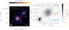 |
Fig. 1 Dust continuum and emission of selected iCOM transitions toward IRAS 4A2. Left: 1.3 mm dust continuum emission in color scale and gray contours. The first contours and steps are 3σ (σ = 0.6 mJy beam−1). The cyan star marks the IRAS 4A2 dust peak, 3h29m10s.431 (RA) and +31° 13′32.″00 (Dec). The beam is 0.″20 × 0.″ 14 (–26°). Right: dust continuum (grayscale) overlaid with moment 0 contours maps of CH3OH 16(–2,15)–15(–3,13) E (green), integrated over +3 to +10 km s−1, CH3CHO 13(0,13)–12(0,12) E [υt=2] (orange), integrated over +4 to +9 km s−1, and CH2OHCHO 34(5,30)–34(4,31) (blue), integrated over +6 to +8 km s−1. The first contours and steps are 3 and 6σ respectively, with σ = 3.7 mJy beam−1 km s−1 for CH3OH, σ = 2.7 mJy beam−1 km s−1 for CH3CHO, and σ = 2.3 mJy beam−1 km s−1 for CH2OHCHO. The beam is 0.″ 17 × 0.″ 12 (–28°). |
3 Results
3.1 Spatial segregation of iCOMs
To study the spatial distribution of the identified iCOMs, we produced and compared integrated intensity maps of different species using isolated transitions with similar Eu so as to avoid excitation biases. Figure 1 shows, on the left, the IRAS 4A system in 1.3 mm dust continuum emission and, on the right, a zoomed-in image of the same map onto IRAS 4A2, with overplotted colored contours of the integrated intensity maps of three selected iCOMs transitions: CH3OH 16(−215)–15(−3,13) E (Eu=338 K); CH3CHO 13(0,13)–12(0,12) E (Eu=461 K); CH2OHCHO 34(5,30)–34(4,31) (Eu=344 K). The moment 0 maps of all the isolated transitions for each species can be seen online6. These maps show that the various iCOMs trace different scales. To quantify this, we estimated the emitting radius associated with each species by performing a 2D Gaussian fit of the emission on the integrated intensity maps using the imfit task in CASA. For the few transitions whose emission is clearly associated with IRAS 4A2 alone, avoiding any contamination from the companion IRAS 4A1, we also performed a Gaussian fit on the visibility plan with the uvmodelfit task in CASA. Since the fit results in the visibility plane are consistent within ± 1−2 au with the image plane determinations, we analyzed all the isolated lines using only the image plane results (see table online). Some examples of the fitted images and of the residual maps are available online. For all transitions, the residual maps of the fit show no emission above 2−3σ. From the beam-deconvolved major (θM) and minor (θm) diameters of the fitted Gaussian ellipses (see table online), we derived a radius of the emitting line as one-half of the geometric average of θM and θm.
Figure 2 shows the beam-deconvolved radius (in au) for each isolated transition versus the line Eu . The iCOMs display different emitting sizes; in other words, the observed transitions must trace a different outer radius in the hot corino, where the line optical depth is equal to or larger than 1. Therefore, the estimated emitting radii within the error bars (shaded regions in Fig. 2) indicate that we are probing different regions of the hot corino of IRAS 4A2, extending out to an outer radius that spans between 16 and 40 au, depending on the considered species. We note, however, that the exact geometry of this molecular emission cannot be unambiguously determined with a 2D Gaussian fit. A higher angular resolution coupled with a detailed chemo-physical model of the molecular line emission are needed to resolve this ambiguity. To estimate the dependence of the emitting size versus the transition, we linearly fitted the derived radius with respect to Eu, except for CH2OHCHO and NH2CHO due to their partially unresolved emission. The fit shows a small variation in the size as a function of Eu, with negative slopes deviating from zero by factors of 0.014 ± 0.003 (CH3OH, = 4.7), 0.04 ± 0.01 (HCOOCH3,
 = 1.0), 0.010 ± 0.0022 ± 0.005 (CH3CHO,
  = 1.4), and 0.016 ± 0.005 (CH3CH2OH;
  = 0.4). We therefore computed a weighted average emission region radius per species (
 ; Table 1) as a representative emitting size.
Another possibility is that we are observing different molecular abundances at limited sensitivity. This means that we are able to detect the less abundant species only at the highest densities, and hence closer to the protostar at small emitting radii. Among the various detected species, methanol (CH3OH) is known to be the most abundant iCOM, and a tracer of the protostellar environment at different scales (e.g., also outflows). Instead, acetaldehyde (CH3CHO), formamide (NH2CHO), and glycolaldehyde (CH2OHCHO) seem to share similar lower abundances, and to only trace the hot corino region (see, e.g., Taquet et al. 2015; López-Sepulcre et al. 2017; Belloche et al. 2020). While we cannot exclude a priori the aforesaid possibility, the fact that we observe a difference in the emitting size for all the iCOMs, also among the compact species, strongly suggests that the observed chemical segregation in IRAS 4A2 is real. In addition, it should be noted that the observed difference in emitting sizes holds independently of the upper-state energy Eu, as we compared different iCOM transitions at similar Eu precisely to account for the gas excitation conditions.
A similar stratification has been observed in two other hot corinos, B335 (Okoda et al. 2022), between CH3OH and NH2CHO, and HH212, with CH3OH, NH2CHO, and CH3CHO, (Lee et al. 2022), and toward some hot cores in high-mass starforming regions (Jiménez-Serra et al. 2012; Calcutt et al. 2014; Gieser et al. 2019; Gieser et al. 2021). Bianchi et al. (2022) and Lee et al. (2022) associated this segregation with the different binding energy of the species. To prove this in IRAS 4A2, binding energies must be consistently derived for all the investigated iCOMs.
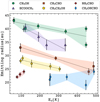 |
Fig. 2 iCOM beam-deconvolved radius as a function of the line upperstate energy. The colored markers correspond to a chosen sample (see Sect. 3.1 and the Appendices online) of imaged and fitted iCOM transitions. The gray solid lines indicate the linear fit performed on the derived radius. The shaded colored regions highlight the emitting regions associated with each iCOM. |
1σ confidence level results of the iCOM molecular lines analysis and line emitting radius fit toward IRAS 4A2.
3.2 Gas temperature and column density estimates
In order to characterize the hot corino species column density and gas temperature, we analyzed the IRAS 4A2 spectrum performing a Gaussian fit on the emitting iCOM lines7. The line peak velocities lie between +5.9 and +7.5 km s−1, consistent with the systemic velocity of IRAS 4A2 (+6.8 km s−1; Choi 2001) given the channel resolution of ~1.4 km s−1. At this spectral resolution we do not detect significant deviations of the line profiles from a thermally broadened Gaussian. We note that we excluded from the analysis heavily blended transitions where we could not disentangle the emission.
The standard rotational diagram (RD) method (Blake et al. 1987; Turner 1991; Goldsmith & Langer 1999; Mangum & Shirley 2015) assumes local thermodynamic equilibrium (LTE) and optically thin line emission. While LTE is generally valid due to the high densities of the probed region (higher than the species critical density; De Simone et al. 2020a, 2022a), the optical depth assumption is likely not applicable for most of the iCOMs targeted here. This can lead to a potential underestimation of the upper-state populations of these transitions (Taquet et al. 2015; De Simone et al. 2020a).
Methanol (CH3OH) is known to be very abundant and optically thick in Class 0 sources, including IRAS 4A2. It is also one of the very few complex organic molecules for which collisional coefficients have been computed in order to perform a non-LTE analysis. We therefore performed a non-LTE analysis via our custom Large Velocity Gradient (LVG) code grelvg (Ceccarelli et al. 2003; De Simone et al. 2020a). With this analysis we fit the observed molecular line intensities and compared them with the predicted values using a chi-square minimization  , accounting for line opacity. More details on the method can be found in Appendix A. Table 1 and Fig. 3 report the 1σ confidence level range for column density and temperature assuming a 0.″3 emitting size, as derived from the CH3OH integrated intensity maps. The resulting reduced chi-square is 0.6. With an LTE rotational diagram, at 1σ the resulting column density is constrained to 0.9–1.0 × 1018 cm−2, and the temperature to 148–168 K. In comparison, the LTE rotational diagram leads to a lower column density by a factor of ~2, while overestimating the temperature by a factor of ~1.3. There are too few detected lines to perform a statistically significant LTE population diagram (PD) analysis.
For the other iCOMs, which all lack collisional coefficients for an LVG analysis, we used where possible the population diagram approach (Goldsmith & Langer 1999), which corrects rotational temperature and column density estimates for the self-consistently estimated line opacity. The methodology is described in detail in Appendix B. It is important to note that lines with high excitation (Eu ≥ 300 K) may not be collisionally dominated, but rather radiatively pumped by the infrared field of the protostar (Tielens 2005). Therefore, they may not represent the actual kinetic temperature of the gas and may bias the population diagram results. Including radiative pumping would require detailed physical and chemical modeling of the envelope, which is beyond the scope of this work. Because of this, to be on the safe side, at first we restricted the analysis to lines with Eu ≤ 300 K (Table B.1 and Fig. B.1), with resulting reduced chi-square values at 1σ of 0.6 (HCOOCH3), 0.4 (CH3CH2OH), and 0.6 (CH2OHCHO). Then we repeated the analysis accounting for all detected lines, including the ones with Eu > 300 K (Fig. 4). We found that the best-fit results for column densities and temperatures are consistent between the two cases. Considering all lines, we obtained 1σ confidence level ranges with  values of 1.0 (HCOOCH3), 0.9 (CH3CH2OH), and 0.5 (CH2OHCHO). The best fits to the population diagram (see Figs. 4 and B.1) are similar in the two cases, implying that the bulk of the emission of the two groups of transitions (with Eu below and above 300 K) can be represented by the same physical conditions. In light of these results, we conclude that, in our case, the radiative pumping contribution may be negligible, and we therefore rely on the results considering all transitions, which also allow more reliable 1σ estimates. We note that for glycolaldehyde (CH2OHCHO) the FAUST data only cover transitions with high Eu . We therefore complemented our dataset with the sample from Taquet et al. (2015) as it covers transitions with Eu below 200 K, accounting for the different beam size (~2″). We confirm that most of the lines are optically thick (τ > 1), justifying the requirement for the population diagram analysis. There are too few acetaldehyde (CH3CHO) transitions to perform a statistically significant PD analysis. Thus, we relied on the RD analysis; the results are reported in Table 1 and Fig. C.1. Finally, the few detected formamide (NH2CHO) lines span a range of Eu that is too small to obtain reliable results from a rotational diagram. Nonetheless, given that NH2CHO traces a similar spatial scale to CH2OHCHO, we derived a lower limit on the column density (see Table 1), assuming the same best-fit temperature derived for CH2OHCHO.
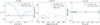 |
Fig. 3 Non-LTE LVG fitting results for methanol (CH3OH) with (full color) and without (shaded) considering the contribution from millimeter foreground dust absorption (see Sect. 3.2). Left: χ2 minimization for the total column density |


4 Discussion
4.1 The effect of millimeter foreground dust absorption
There are several possible mechanisms by which the observed molecular line emission may be obscured or otherwise reduced in the presence of optically thick dust. First, Class 0/I sources may be embedded in envelopes which often are optically thick at millimeter or sub-millimeter wavelengths (Miotello et al. 2014; Galván-Madrid et al. 2018; Galametz et al. 2019). In this case, the foreground dust may absorb the molecular emission, what we call here millimeter dust obscuration. This leads to a nondetection of iCOMs at millimeter wavelengths (e.g., López-Sepulcre et al. 2017; De Simone et al. 2017; Belloche et al. 2020), to the underestimation of the molecular column density inferred from optically thin lines, or to an underestimation of both column density and temperature when the optical depth of the lines is non-negligible (De Simone et al. 2020a). Even if the dust is co-spatial with the gas, in the case of optically thick dust and LTE molecules in emission, the line emission will be inseparable from the dust continuum emission. Therefore, the process of continuum subtraction will result in reduced (or apparently absent or negative) line emission, regardless of the lines being intrinsically optically thin or optically thick.
As another possibility, if the molecular gas resides in front of optically thick dust continuum emission, then after continuum subtraction the molecular lines may appear either in emission or absorption, or not appear at all, depending on the relative brightness temperatures of the line- and the dust-emitting regions. It can be difficult to distinguish between these scenarios without considering additional information about the source of the emission. Nevertheless, in all cases the derived molecular column densities and excitation temperatures can be significantly underestimated if the dust emission is not taken into account.
De Simone et al. (2020a, 2022b) uniquely estimated, using a combination of centimeter and millimeter observations, that the foreground dust may absorb the emission lines in IRAS 4A2 on scales of 0.″26, about 30% at 143 GHz and 50% at 243 GHz. Assuming that all species on scales <0.″26 will be affected in some way by millimeter dust obscuration, we corrected the integrated line flux for these factors (see the results in Table 1). In the PD and the LVG analysis, we found a systematic shift toward higher temperatures of 50–100 K and higher column densities by a factor of about 1.6 (2.2 for CH3CH2OH). For acetaldehyde (CH3CHO) and formamide (NH2CHO) we found a similar increase in column density from the RD analysis.
We compared our estimates to the literature values (Taquet et al. 2015; De Simone et al. 2017, 2020a; López-Sepulcre et al. 2017; Belloche et al. 2020). In particular, Belloche et al. (2020) were the first to isolate IRAS 4A2 as a compact hot corino; however, higher spatial resolution, as we achieved with this work, was necessary to spatially resolve the emitting size of various iCOMs. The values derived for methanol (CH3OH) correcting for dust obscuration are consistent at 1σ ( ) with those derived at centimeter wavelengths by De Simone et al. (2020a). The foreground dust absorption affects column density and temperature similarly to the line opacity (respectively with increasing factors of ~1.4 and ~3), with respect to the LTE rotational diagram method. For the other iCOMs, our new estimates generally point toward higher column densities and higher temperatures than previously measured. These discrepancies are due to a combination of line optical depth and foreground dust absorption effects.
Taking into account the foreground dust absorption and the measured line opacities, we do not observe systematic differences for line widths and position angles among the different molecular species8. Only CH3OH shows slightly larger line widths, on average ~4 km s−1 instead of ~3.5 km s−1 as for the other species. This could be due to the fact that methanol’s transitions may trace, particularly at low upper-state energy, other physical processes in the protostellar environment such as outflowing material (e.g., De Simone et al. 2024). From the measured position angles, we estimate an inclination angle in the range of 11–56 degrees. However, the measured line widths and position angles are uncertain and the error bars, especially for the latter, are often large. A larger spectral resolution is required to conduct a detailed study of the kinematics of the IRAS 4A system.
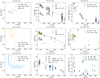 |
Fig. 4 LTE population diagrams (PD) of methyl formate (HCOOCH3), ethanol (CH3CH2OH), and glycolaldehyde (CH2OHCHO). For CH2OHCHO, we complemented our dataset (blue diamonds) with the dataset of Taquet et al. (2015) (green diamonds). The results are plotted with (shaded) and without (full color) the millimeter dust obscuration factor. Left: column density-temperature reduced |

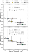 |
Fig. 5 T–r profile of IRAS 4A2. The gas temperatures are derived accounting for all transitions and for the millimeter dust obscuration (bottom). The colored data points mark the best-fit gas temperature derived for each species as a function of the average emitting radius r̄. The emitting radius error bar encompasses the observed range of sizes per species. The error bar on the temperature is the 1σ confidence range of the LTE rotational diagram analysis (CH3CHO), of the LTE population diagram analysis (HCOOCH3, CH3CH2OH, and CH2OHCHO), and of the non-LTE LVG analysis for CH3OH. The gray solid line in both panels is the best fit to the data points excluding CH3CHO (see Sect. 3.2). |
4.2 The gas temperature profile of the IRAS 4A2 hot corino
The iCOM spatial segregation together with the temperature estimate allow us to tentatively derive the gas temperature profile of IRAS 4A2 as a function of radial distance. Figure 5 shows the derived gas temperatures (with and without accounting for the millimeter dust obscuration) versus the deconvolved emitting size derived for each species as a probe of the distance from the protostellar center. For completeness, Fig. C.2 shows the resulting temperature profile accounting only for iCOM transitions with Eu ≤ 300 K. We naturally excluded from the fit formamide (NH2CHO), for which it was not possible to reliably estimate the rotational temperature, and acetaldehyde (CH3CHO), for which we could not estimate self-consistently the contribution of the line opacity. Nevertheless, we included as a reference the CH3CHO temperature derived with the RD in Fig. 5.
From theory, the dust temperature is expected to radially behave as a power law: T(r) ∝ rq (Beckwith et al. 1990; Motte & André 2001; Andrews & Williams 2007). At high densities, such as in hot corinos, gas and dust are likely thermally coupled (Ceccarelli et al. 1996; Maret et al. 2002; Crimier et al. 2009; Crimier et al. 2010). By fitting the data points with a power-law function, we find an exponent q = −1.0 ± 0.2. Accounting for the millimeter dust obscuration, we obtain a consistent result of q = −0.8 ± 0.2. A similar attempt in low-mass protostars has been performed at larger scales, focusing on modeling and/or observing simpler molecular species (e.g., CO, H2CO, H2CS) and hinting to a profile of spherically collapsing envelopes (Ceccarelli et al. 2000; Maret et al. 2002; Crimier et al. 2010), or rotationally supported disk (Jacobsen et al. 2018; van’t Hoff et al. 2020). Our fit implies a power law steeper than expected in an optically thin spherical collapsing envelope (q ~0.4–0.5; Ceccarelli et al. 2000; Schöier et al. 2002; Crimier et al. 2010). Alternatively, we might be observing layers in the envelope where the dust optical depth is ≤ 1 (Adams & Shu 1986; Ceccarelli et al. 1996). From the comparison with observations at centimeter wavelengths, De Simone et al. (2020a) estimated a dust foreground absorption of 30% circa, which corresponds to a dust optical depth of about 0.3. This is reasonable since a completely optically thick envelope (τ > 1) would have completely absorbed the molecular line emission, as in the case of the IRAS 4A1 binary component (De Simone et al. 2020a). Another possibility to explain the high gas temperature observed at these compact scales is that the iCOMs are probing a disk-like structure that is gravitationally unstable Zamponi et al. (2021).
To untangle which contribution dominates, we need a detailed thermochemical model to reproduce the T–r profile, and high angular (about 5–10 au) observations at higher spectral resolution so as to resolve the kinematics of the most compact iCOM species.
5 Conclusions
Within the FAUST framework we observed for the first time a chemical segregation of six iCOMs in the IRAS 4A2 hot corino. Our conclusions can be summarized as follows:
The detected iCOMs show different emitting sizes of increasing outer radius, with methanol (CH3OH) being the most extended, at ~40 au; glycolaldehyde (CH2OHCHO) and formamide (NH2CHO) the most compact and partially unresolved, at ~22–23 au; and methyl formate (HCOOCH3), acetaldehyde (CH3CHO), and ethanol (CH3CH2OH) in between, with an outer radius located at ~28–36 au;
Using a multi-line analysis, both in LTE and non-LTE (the latter only for CH3OH), we derived gas temperatures and molecular column densities corrected for (i) the line opacity and for (ii) the foreground dust absorption at millimeter wavelengths. The latter implies higher gas temperatures by 50–100 K, and higher column densities by a factor of ~1.6;
We retrieved a gas temperature profile (T–r) at scales of 20–50 au (in radius) directly from the observed molecular line emission. The higher gas temperature (up to 200–250 K) is associated with the more compact iCOM emission. The power-law T–r exponent q ranges from −0.8 to −1.0, inconsistent with an optically thin spherical collapsing envelope. This may hint at a partially optically thick protostellar envelope, or a gravitationally unstable disk-like structure in IRAS 4A2.
At millimeter wavelengths, the optical thickness of foreground dust and the molecular line opacity are crucial parameters to determine unbiased gas temperatures and molecular abundances. This work highlights how the millimeter dust opacity affects not only the estimates of the column densities or the abundances of the observed molecular species, but also the temperature of the traced gas. This is particularly evident for the more abundant species, such as methanol (Ch3OH), which has optically thick emission lines. However, high spatial and spectral resolution observations, paired with a large bandwidth, are still needed to spatially resolve the molecular emission as well as the gas kinematics, especially of the most compact iCOM species. This will also allow us to clarify the exact source geometry.
This work opens the way to many future perspectives. First of all, there is a need to derive similar temperature profiles for other Class 0/I protostars, and compare them with the predictions on embedded young disks from the latest simulations (e.g., Lebreuilly et al. 2024). Also, as mentioned in Sect. 3.1, there is a need to link the stratified chemical structure to the iCOMs binding energies, and perform a similar study on other hot corino sources, which also implies follow-ups at higher angular resolution. This work also sets the ground for the upcoming centimeter facilities (e.g., SKA9 and ngVLA10), as well as the new ALMA wideband sensitivity upgrade (Ossenkopf-Okada et al. 2023). Centimeter observations are particularly crucial to fully characterize hot corinos both from a chemical and physical prospective. With SKA and ngVLA, we will access much larger and complex iCOM species than methanol in a wavelength regime where the dust is more likely optically thin, and spectral line blending and line confusion are reduced. At the same time, ALMA WSU will provide us with a large bandwidth to detect more transitions per species, and therefore perform a more robust multi-line analysis.
Data availability
The ALMA observations used in this manuscript are publicly available on the ALMA archive. The appendices related to line spectra, their spectral parameters, fit results, and the results from image plane fitting of chosen line are openly available on Zenodo at https://doi.org/10.5281/zenodo.14780814.
Acknowledgements
We thank the anonymous referee for all the useful comments and suggestions that greatly improved the manuscript. This Paper makes use of the following ALMA data: ADS/JAO.ALMA#2018.1.01205.L (PI: S. Yamamoto). ALMA is a partnership of the ESO (representing its member states), the NSF (USA) and NINS (Japan), together with the NRC (Canada) and the NSC and ASIAA (Taiwan), in cooperation with the Republic of Chile. The Joint ALMA Observatory is operated by the ESO, the AUI/NRAO, and the NAOJ. This work was partly supported by the Italian Ministero dell Istruzione, Università e Ricerca through the grant Progetti Premiali 2012 – iALMA (CUP C52I13000140001). This project has received funding from the European Union's Horizon 2020 research and innovation programme under the Marie Sklodowska-Curie grant agreement No 823823 (DUSTBUSTERS) and from the European Research Council (ERC) via the ERC Synergy Grant ECOGAL (grant 855130). Part of the analysis and work that led to this study were carried out during the May 2023 workshop at the Institut Pascal in Saclay, which was funded and organized as part of the ECOGAL collaboration. JF acknowledges financial support from the DIFA and the ESO Office for Science. ClCO, LP, GS and EB acknowledge the PRIN-MUR 2020 BEYOND-2p (Astrochemistry beyond the Second period elements, Prot. 2020AFB3FX), the project ASI-Astrobiologia 2023 MIGLIORA (Modeling Chemical Complexity, F83C23000800005), the INAF-GO 2023 fundings PROTO-SKA (Exploiting ALMA data to study planet-forming disks: preparing the advent of SKA, C13C23000770005), the INAF Mini-Grant 2022 "Chemical Origins" (PI: L. Podio), the INAF Mini-grant 2023 TRIESTE ("TRacing the chemIcal hEritage of our originS: from proTostars to planEts"; PI: G. Sabatini), and the National Recovery and Resilience Plan (NRRP), Mission 4, Component 2, Investment 1.1, Call for tender No. 104 published on 2.2.2022 by the Italian Ministry of University and Research (MUR), funded by the European Union – NextGenerationEU – Project Title 2022JC2Y93 Chemical Origins: linking the fossil composition of the Solar System with the chemistry of protoplanetary disks – CUP J53D23001600006 – Grant Assignment Decree No. 962 adopted on 30.06.2023 by the Italian Ministry of Ministry of University and Research (MUR). E.B. also acknowledges the contribution of the Next Generation EU funds within the National Recovery and Resilience Plan (PNRR), Mission 4 – Education and Research, Component 2 – From Research to Business (M4C2), Investment Line 3.1 – Strengthening and creation of Research Infrastructures, Project IR0000034 – "STILES – Strengthening the Italian Leadership in ELT and SKA". I.J.-S. acknowledges funding from grant PID2022-136814NB-I00 funded by MICIU/AEI/10.13039/501100011033 and by "ERDF/EU". SBC was supported by the NASA Planetary Science Division Internal Scientist Funding Program through the Fundamental Laboratory Research work package (FLaRe). M.B. acknowledges the support from the European Research Council (ERC) Advanced Grant MOPPEX 833460.
Appendix A Non-LTE LVG analysis for CH3OH
Since methanol (CH3OH) is known to be very abundant in this source (see, e.g., De Simone et al. 2020a) and optically thick, to complement and check the analysis made with the LTE and optically thin line assumptions, we performed a non-LTE analysis using a Large Velocity Gradient (LVG) code (Ceccarelli et al. 2003). We could therefore derive the physical properties of the gas emitting CH3OH, namely gas temperature, density and column density, and the optical depth of the transitions. We used the collisional coefficients of both A-type and E-type of CH3OH with para-H2, computed by Rabli & Flower (2010) between 10 and 200 K for the first 256 levels and provided by the BASecOL database (Dubernet et al. 2013). We note that, given that the coefficient are available only for transition with J up to 15 and computed for temperatures up 200 K, we used the transitions that in this work have Eu less than 200 K. For this purpose we added the transition identified in the narrow SPW centered at 244 GHz, identified as 5(1,3) −4(1,3) A with the following spectroscopic and Gaussian parameters: Eu = 50 K; Log10Aul= −4.7; gu = 44; W = 340 ± 10 K km s−1; Vpeak = 6.74 ± 0.08 km s−1; FWHM = 5.8 ± 0.2 km s−1. We assumed a spherical geometry to compute the line escape probability, the CH3OH-A/CH3OH-E ratio equal to 1, and the H2 ortho-to-para ratio equal to 3. We ran a large rid of models (~ 13 000) covering the frequency of the observed CH3OH lines, a total (A-type plus E-type) column density  from 1016 to 4 × 1019 cm−2, a gas density
  from 106 to 2 × 108 cm−3, both sampled in logarithmic scale, and a gas temperature T from 80 to 190 K, sampled in linear scale. We then simultaneously fitted the measured CH3OH-A and CH3OH-E line intensities via comparison with those simulated by the LVG model, leaving
  , and T as free parameters. Following the observations, we assumed a source size of 0″.3 to compute the filling factor, a line width equal to 4.5 km s−1, and we included the calibration/continuum subtraction uncertainty (20%) in the observed intensities.
The chi-square best fit is obtained for a total CH3OH column density of 2 × 1018 cm−2, a gas temperature of 100 K and gas density of 2 × 106 cm−3, with reduced chi-square  . Finally, we corrected the intensities for the foreground dust absorption. In this case, the best fit is obtained for a total CH3OH column density of 4 × 1018 cm−2, a gas temperature of 150 K and gas density of 5 × 106 cm−3, with reduced chi-square
  . The results do not change assuming a line width ±0.5 km s−1 with respect to the chosen one. Figure 3 shows the density-temperature χ2 surface of the
  best fit. The fit results in the 1σ confidence range are reported in Tab. 1.
Appendix B LTE population diagram analysis
We performed a population diagram analysis on methyl formate (HCOOCH3), ethanol (CH3CH2OH), and glycolaldehyde (CH2OHCHO) to correct rotational temperature Trot and total column density Ntot for the line optical depth (τ), following the prescription of Goldsmith & Langer (1999). The optical depth of a transition can be written as
 (B.1)
(B.1)

In the above, c is the speed of light, v0 the rest-frame line frequency, Aul the Einstein coefficient for spontaneous emission, Δv the line profile FWHM (derived by fitting the line with a gaussian profile), gu the statistical weight of the upper state, Eu the upper-state energy of the transition, h and k respectively the Planck and the Boltzmann constants, W the velocity-integrated line intensity, and f f the beam filling factor, defined as:  (e.g., Mangum & Shirley 2015). θbeam is the synthesized beam of the observations. All units refer to the cgs system.
Finally, Cτ is the optical depth correction factor:
 (B.3)
(B.3)
This factor indicates how much the upper level populations (Nu) are underestimated due to the line opacity. When the line is optically thin, Cτ is equal to unity.
For a molecule in LTE, all excitation temperatures are the same, and the population of each level is given by
 (B.4)
(B.4)
where Ntot the species total column density, and Q(Trot) the partition function at the rotational temperature Trot of the species.
We created a 2D parameter space grid in rotational temperature (50 values between 50 and 500 K), and in total column density (50 values between 1 × 10¹⁶ and 5 × 1019 cm−2) at fixed source size θsource (see Table 1). For each set of Trot and Ntot we computed the model upper state column densities Nu, model using equation B.3, as well as the line opacity τ (Eq. B.1) and the resulting Cτ (Eq. B.3). Then we retrieved the corrected upper state column densities Nu, corr using Eq. B.2, in which the observed velocity-integrate integrated line intensities are corrected for the beam dilution and the opacity factor. Finally, we performed a chi-square minimization test comparing Nu, corr and Nu, model:
 (B.5)
(B.5)
Here N is the number of observed lines, while σ is the observed error on ln(Nu/gu), calculated as
 (B.6)
(B.6)
where ΔW is the error on the fitted line intensities,11 and σf is the absolute flux calibration error, that we fixed as 20% of W. In Figs. 4 and B.1, respectively, we report the results of this analysis accounting respectively for all transitions and the low-excitation ones (Eu < 300 K) only.
Accounting solely for lines with Eu ≤ 300 K (see Tab. B.1), Trot and Ntot are strongly degenerate in the case of HCOOCH3 and CH2OHCHO, and less degenerate for CH3CH2OH. The resulting minimum  is 0.6 (HCOOCH3), 0.4 (CH3CH2OH), and 0.6 (CH2OHCHO). We could extract only a lower limit on the temperature for HCOOCH3, and a lower limit on the total column density for CH3CH2OH and CH2OHCHO.
The inclusion of high-excitation lines (Fig. 4) helps closing the  contours within the investigated parameter space, and to attenuate the degeneracy between Trot, Ntot and τ. The minimum
  in this case is 1.0 (HCOOCH3), 0.9 (CH3CH2OH), and 0.5 (CH2OHCHO).
Accounting for a 50% millimeter dust obscuration factor12 on the velocity-integrated line intensities, the effect is to increase the best-fit temperature range by 50-100 K within error bars, and increase the total column density by a factor of about 1.6 (2.2 for CH3CH2OH). The best-fit  is 0.6 (HCOOCH3), 0.6 (CH3CH2OH), and 0.6 (CH2OHCHO) for Eu < 300 K, and 1.4 (HCOOCH3), 1.3 (CH3CH2OH), and 0.5 (CH2OHCHO) using all lines. The effect on the line optical depth is to change the average line opacity by 0.4 dex (Eu < 300 K) and 0.1 dex (all lines).
1σ confidence level results of the population diagram analysis with Eu < 300 K.
Appendix C Additional notes and results
Figure C.1 shows the rotational diagram of CH3CHO computed using all lines13, and correcting for the derived source size of 0″.20. Shaded data points and solid line take into account the millimeter dust obscuration (see Sect. 4.1). The best-fit results in both cases are reported in Tab. 1.
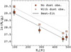 |
Fig. C.1 Rotational diagram (RD) of CH3CHO. The solid gray line is the best fit to the data points with (shaded) and without (full color) millimeter dust obscuration factor. The upper-state column densities are corrected for beam dilution. |
Figure C.2 shows the gas radial temperature profile of IRAS 4A2 obtained from the population diagram analysis of HCOOCH3, CH3CH2OH, and CH2OHCHO below 300 K, and the non-LTE LVG analysis of CH3OH. CH3CHO and NH2CHO are here not reported, as it was not possible to perform a conservative line analysis or obtain an independent estimate of the gas temperature, respectively. The gray dotted line refers to the best fit to the data points of the top panel in Fig. 5.
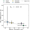 |
Fig. C.2 Same as Fig. 5, but for iCOMs transitions with Eu < 300 K. The arrow indicates a lower limit on the temperature. The gray dotted line is the best fit to the data points in the top panel of Fig. 5). |
References
- Adams, F. C., & Shu, F. H. 1986, ApJ, 308, 836 [NASA ADS] [CrossRef] [Google Scholar]
- André, P. 2002, EAS Publ. Ser., 3, 1 [CrossRef] [EDP Sciences] [Google Scholar]
- André, P., Ward-Thompson, D., & Barsony, M. 2000, in Protostars and Planets IV, eds. V. Mannings, A. P. Boss, & S. S. Russell, 59 [Google Scholar]
- Andrews, S. M., & Williams, J. P. 2007, ApJ, 659, 705 [NASA ADS] [CrossRef] [Google Scholar]
- Beckwith, S. V. W., Sargent, A. I., Chini, R. S., & Guesten, R. 1990, AJ, 99, 924 [Google Scholar]
- Belloche, A., Maury, A. J., Maret, S., et al. 2020, A&A, 635, A198 [NASA ADS] [CrossRef] [EDP Sciences] [Google Scholar]
- Bernabò, L. M., Turrini, D., Testi, L., Marzari, F., & Polychroni, D. 2022, ApJ, 927, L22 [CrossRef] [Google Scholar]
- Bianchi, E., López-Sepulcre, A., Ceccarelli, C., et al. 2022, ApJ, 928, L3 [NASA ADS] [CrossRef] [Google Scholar]
- Blake, G. A., Sutton, E. C., Masson, C. R., & Phillips, T. G. 1987, ApJ, 315, 621 [Google Scholar]
- Bottinelli, S., Ceccarelli, C., Lefloch, B., et al. 2004, ApJ, 615, 354 [Google Scholar]
- Calcutt, H., Viti, S., Codella, C., et al. 2014, MNRAS, 443, 3157 [Google Scholar]
- Caselli, P., & Ceccarelli, C. 2012, A&AR, 20, 56 [NASA ADS] [CrossRef] [Google Scholar]
- Ceccarelli, C. 2004, in Star Formation in the Interstellar Medium: In Honor of David Hollenbach, eds. D. Johnstone, F. C. Adams, D. N. C. Lin, D. A. Neufeeld, & E. C. Ostriker, Astronomical Society of the Pacific Conference Series, 323, 195 [NASA ADS] [Google Scholar]
- Ceccarelli, C. 2023, in The Interplay of Dust, European Conference on Laboratory Astrophysics ECLA2020, 3 [NASA ADS] [CrossRef] [Google Scholar]
- Ceccarelli, C., Hollenbach, D. J., & Tielens, A. G. G. M. 1996, ApJ, 471, 400 [Google Scholar]
- Ceccarelli, C., Castets, A., Caux, E., et al. 2000, A&A, 355, 1129 [NASA ADS] [Google Scholar]
- Ceccarelli, C., Maret, S., Tielens, A. G. G. M., Castets, A., & Caux, E. 2003, A&A, 410, 587 [NASA ADS] [CrossRef] [EDP Sciences] [Google Scholar]
- Ceccarelli, C., Caselli, P., Fontani, F., et al. 2017, ApJ, 850, 176 [NASA ADS] [CrossRef] [Google Scholar]
- Ceccarelli, C., Codella, C., Balucani, N., et al. 2023, in Protostars and Planets VII, eds. S. Inutsuka, Y. Aikawa, T. Muto, K. Tomida, & M. Tamura, Astronomical Society of the Pacific Conference Series, 534, 379 [NASA ADS] [Google Scholar]
- Chahine, L., Ceccarelli, C., De Simone, M., et al. 2024, MNRAS, 531, 2653 [NASA ADS] [CrossRef] [Google Scholar]
- Choi, M. 2001, ApJ, 553, 219 [NASA ADS] [CrossRef] [Google Scholar]
- Codella, C., Ceccarelli, C., Chandler, C., et al. 2021, Front. Astron. Space Sci., 8, 227 [NASA ADS] [CrossRef] [Google Scholar]
- Crimier, N., Ceccarelli, C., Lefloch, B., & Faure, A. 2009, A&A, 506, 1229 [NASA ADS] [CrossRef] [EDP Sciences] [Google Scholar]
- Crimier, Ceccarelli, C., Alonso-Albi, T., et al. 2010, A&A, 516, A102 [NASA ADS] [CrossRef] [EDP Sciences] [Google Scholar]
- De Simone, M., Codella, C., Testi, L., et al. 2017, A&A, 599, A121 [NASA ADS] [CrossRef] [EDP Sciences] [Google Scholar]
- De Simone, M., Ceccarelli, C., Codella, C., et al. 2020a, ApJ, 896, L3 [NASA ADS] [CrossRef] [Google Scholar]
- De Simone, M., Ceccarelli, C., Codella, C., et al. 2022a, ApJ, 935, L14 [CrossRef] [Google Scholar]
- De Simone, M., Codella, C., Ceccarelli, C., et al. 2020b, A&A, 640, A75 [NASA ADS] [CrossRef] [EDP Sciences] [Google Scholar]
- De Simone, M., Ceccarelli, C., Codella, C., et al. 2022a, ApJ, 935, L14 [CrossRef] [Google Scholar]
- De Simone, M., Codella, C., Ceccarelli, C., et al. 2022b, MNRAS, 512, 5214 [CrossRef] [Google Scholar]
- De Simone, M., Podio, L., Chahine, L., et al. 2024, A&A, 686, L13 [NASA ADS] [CrossRef] [EDP Sciences] [Google Scholar]
- Dubernet, M. L., Alexander, M. H., Ba, Y. A., et al. 2013, A&A, 553, A50 [NASA ADS] [CrossRef] [EDP Sciences] [Google Scholar]
- Galametz, M., Maury, A. J., Valdivia, V., et al. 2019, A&A, 632, A5 [NASA ADS] [CrossRef] [EDP Sciences] [Google Scholar]
- Galván-Madrid, R., Liu, H. B., Izquierdo, A. F., et al. 2018, ApJ, 868, 39 [CrossRef] [Google Scholar]
- Gieser, C., Semenov, D., Beuther, H., et al. 2019, A&A, 631, A142 [NASA ADS] [CrossRef] [EDP Sciences] [Google Scholar]
- Gieser, C., Beuther, H., Semenov, D., et al. 2021, A&A, 648, A66 [EDP Sciences] [Google Scholar]
- Goldsmith, P. F., & Langer, W. D. 1999, ApJ, 517, 209 [Google Scholar]
- Herbst, E., & van Dishoeck, E. F. 2009, ARA&A, 47, 427 [NASA ADS] [CrossRef] [Google Scholar]
- Jacobsen, Jørgensen, J. K., van der Wiel, M. H. D., et al. 2018, A&A, 612, A72 [NASA ADS] [CrossRef] [EDP Sciences] [Google Scholar]
- Jiménez-Serra, I., Zhang, Q., Viti, S., Martín-Pintado, J., & de Wit, W.-J. 2012, ApJ, 753, 34 [CrossRef] [Google Scholar]
- Johansen, A., Blum, J., Tanaka, H., et al. 2014, in Protostars and Planets VI, eds. H. Beuther, R. S. Klessen, C. P. Dullemond, & T. Henning, 547 [Google Scholar]
- Karska, Herczeg, G. J., van Dishoeck, E. F., et al. 2013, A&A, 552, A141 [NASA ADS] [CrossRef] [EDP Sciences] [Google Scholar]
- Kristensen, van Dishoeck, E. F., Bergin, E. A., et al. 2012, A&A, 542, A8 [NASA ADS] [CrossRef] [EDP Sciences] [Google Scholar]
- Lada, C. J. 1987, in Star Forming Regions, 115, eds. M. Peimbert, & J. Jugaku, 1 [NASA ADS] [Google Scholar]
- Lebreuilly, U., Hennebelle, P., Colman, T., et al. 2021, ApJ, 917, L10 [NASA ADS] [CrossRef] [Google Scholar]
- Lebreuilly, U., Hennebelle, P., Colman, T., et al. 2024, A&A, 682, A30 [NASA ADS] [CrossRef] [EDP Sciences] [Google Scholar]
- Lee, C.-F., Codella, C., Ceccarelli, C., & López-Sepulcre, A. 2022, ApJ, 937, 10 [NASA ADS] [CrossRef] [Google Scholar]
- López-Sepulcre, Sakai, N., Neri, R., et al. 2017, A&A, 606, A121 [NASA ADS] [CrossRef] [EDP Sciences] [Google Scholar]
- Manara, C. F., Morbidelli, A., & Guillot, T. 2018, A&A, 618, L3 [NASA ADS] [CrossRef] [EDP Sciences] [Google Scholar]
- Mangum, J. G., & Shirley, Y. L. 2015, PASP, 127, 266 [Google Scholar]
- Maret, S., Ceccarelli, C., Caux, E., Tielens, A. G. G. M., & Castets, A. 2002, A&A, 395, 573 [NASA ADS] [CrossRef] [EDP Sciences] [Google Scholar]
- Maureira, M. J., Gong, M., Pineda, J. E., et al. 2022, ApJ, 941, L23 [NASA ADS] [CrossRef] [Google Scholar]
- Maury, A. J., Belloche, A., André, P., et al. 2014, A&A, 563, L2 [NASA ADS] [CrossRef] [EDP Sciences] [Google Scholar]
- Miotello, A., Testi, L., Lodato, G., et al. 2014, A&A, 567, A32 [NASA ADS] [CrossRef] [EDP Sciences] [Google Scholar]
- Motte, & André. 2001, A&A, 365, 440 [NASA ADS] [CrossRef] [EDP Sciences] [Google Scholar]
- Müller, H. S. P., Schlöder, F., Stutzki, J., & Winnewisser, G. 2005, J. Mol. Struct., 742, 215 [Google Scholar]
- Öberg, K. I., & Bergin, E. A. 2021, Phys. Rep., 893, 1 [Google Scholar]
- Okoda, Y., Oya, Y., Imai, M., et al. 2022, ApJ, 935, 136 [CrossRef] [Google Scholar]
- Ortiz-León, G. N., Loinard, L., Dzib, S. A., et al. 2018, ApJ, 869, L33 [Google Scholar]
- Ossenkopf-Okada, V., Schaaf, R., Breloy, I., & Stutzki, J. 2023, Physics and chemistry of star formation : the dynamical ISM across time and spatial scales: proceedings of the 7th Chile-Cologne-Bonn-Symposium (Köln: Universitäts- und Stadtbibliothekj) [Google Scholar]
- Pickett, H., Poynter, R., Cohen, E., et al. 1998, JQSRT, 60, 883 [NASA ADS] [CrossRef] [Google Scholar]
- Rabli, D., & Flower, D. R. 2010, MNRAS, 406, 95 [Google Scholar]
- Schöier, F. L., Jørgensen, J. K., van Dishoeck, E. F., & Blake, G. A. 2002, A&A, 390, 1001 [NASA ADS] [CrossRef] [EDP Sciences] [Google Scholar]
- Sheehan, P. D., & Eisner, J. A. 2018, ApJ, 857, 18 [NASA ADS] [CrossRef] [Google Scholar]
- Taquet, V., López-Sepulcre, A., Ceccarelli, C., et al. 2015, ApJ, 804, 81 [Google Scholar]
- Tielens, A. G. G. M. 2005, The Physics and Chemistry of the Interstellar Medium [Google Scholar]
- Tung, N.-D., Testi, L., Lebreuilly, U., et al. 2024, A&A, 684, A36 [NASA ADS] [CrossRef] [EDP Sciences] [Google Scholar]
- Turner, B. E. 1991, ApJS, 76, 617 [NASA ADS] [CrossRef] [Google Scholar]
- Tychoniec, L., Manara, Carlo F., Rosotti, Giovanni P., et al. 2020, A&A, 640, A19 [NASA ADS] [CrossRef] [EDP Sciences] [Google Scholar]
- van ‘t Hoff, M. L. R., van Dishoeck, Ewine F., Jørgensen, Jes K., & Calcutt, Hannah. 2020, A&A, 633, A7 [CrossRef] [EDP Sciences] [Google Scholar]
- Zamponi, J., Maureira, M. J., Zhao, B., et al. 2021, MNRAS, 508, 2583 [NASA ADS] [CrossRef] [Google Scholar]
- Zucker, C., Schlafly, E. F., Speagle, J. S., et al. 2018, ApJ, 869, 83 [NASA ADS] [CrossRef] [Google Scholar]
30%, according to De Simone et al. (2020a), for the sample of CH2OHCHO lines from Taquet et al. (2015).
All Tables
1σ confidence level results of the iCOM molecular lines analysis and line emitting radius fit toward IRAS 4A2.
1σ confidence level results of the population diagram analysis with Eu < 300 K.
All Figures
|
Fig. 1 Dust continuum and emission of selected iCOM transitions toward IRAS 4A2. Left: 1.3 mm dust continuum emission in color scale and gray contours. The first contours and steps are 3σ (σ = 0.6 mJy beam−1). The cyan star marks the IRAS 4A2 dust peak, 3h29m10s.431 (RA) and +31° 13′32.″00 (Dec). The beam is 0.″20 × 0.″ 14 (–26°). Right: dust continuum (grayscale) overlaid with moment 0 contours maps of CH3OH 16(–2,15)–15(–3,13) E (green), integrated over +3 to +10 km s−1, CH3CHO 13(0,13)–12(0,12) E [υt=2] (orange), integrated over +4 to +9 km s−1, and CH2OHCHO 34(5,30)–34(4,31) (blue), integrated over +6 to +8 km s−1. The first contours and steps are 3 and 6σ respectively, with σ = 3.7 mJy beam−1 km s−1 for CH3OH, σ = 2.7 mJy beam−1 km s−1 for CH3CHO, and σ = 2.3 mJy beam−1 km s−1 for CH2OHCHO. The beam is 0.″ 17 × 0.″ 12 (–28°). |
| In the text | |
|
Fig. 2 iCOM beam-deconvolved radius as a function of the line upperstate energy. The colored markers correspond to a chosen sample (see Sect. 3.1 and the Appendices online) of imaged and fitted iCOM transitions. The gray solid lines indicate the linear fit performed on the derived radius. The shaded colored regions highlight the emitting regions associated with each iCOM. |
| In the text | |
|
Fig. 3 Non-LTE LVG fitting results for methanol (CH3OH) with (full color) and without (shaded) considering the contribution from millimeter foreground dust absorption (see Sect. 3.2). Left: χ2 minimization for the total column density |
| In the text | |
|
Fig. 4 LTE population diagrams (PD) of methyl formate (HCOOCH3), ethanol (CH3CH2OH), and glycolaldehyde (CH2OHCHO). For CH2OHCHO, we complemented our dataset (blue diamonds) with the dataset of Taquet et al. (2015) (green diamonds). The results are plotted with (shaded) and without (full color) the millimeter dust obscuration factor. Left: column density-temperature reduced |
| In the text | |
|
Fig. 5 T–r profile of IRAS 4A2. The gas temperatures are derived accounting for all transitions and for the millimeter dust obscuration (bottom). The colored data points mark the best-fit gas temperature derived for each species as a function of the average emitting radius r̄. The emitting radius error bar encompasses the observed range of sizes per species. The error bar on the temperature is the 1σ confidence range of the LTE rotational diagram analysis (CH3CHO), of the LTE population diagram analysis (HCOOCH3, CH3CH2OH, and CH2OHCHO), and of the non-LTE LVG analysis for CH3OH. The gray solid line in both panels is the best fit to the data points excluding CH3CHO (see Sect. 3.2). |
| In the text | |
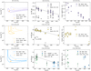 |
Fig. B.1 Same as Fig. 4, but for lines with Eu < 300 K. |
| In the text | |
|
Fig. C.1 Rotational diagram (RD) of CH3CHO. The solid gray line is the best fit to the data points with (shaded) and without (full color) millimeter dust obscuration factor. The upper-state column densities are corrected for beam dilution. |
| In the text | |
|
Fig. C.2 Same as Fig. 5, but for iCOMs transitions with Eu < 300 K. The arrow indicates a lower limit on the temperature. The gray dotted line is the best fit to the data points in the top panel of Fig. 5). |
| In the text | |
Current usage metrics show cumulative count of Article Views (full-text article views including HTML views, PDF and ePub downloads, according to the available data) and Abstracts Views on Vision4Press platform.
Data correspond to usage on the plateform after 2015. The current usage metrics is available 48-96 hours after online publication and is updated daily on week days.
Initial download of the metrics may take a while.