| Issue |
A&A
Volume 692, December 2024
|
|
|---|---|---|
| Article Number | A117 | |
| Number of page(s) | 12 | |
| Section | Astrophysical processes | |
| DOI | https://doi.org/10.1051/0004-6361/202452132 | |
| Published online | 05 December 2024 | |
Unveiling the rebrightening mechanism of GRS 1915+105: Insights from a change in the quasi-periodic oscillations and from a wind analysis
1
Institut für Astronomie und Astrophysik, Kepler Center for Astro and Particle Physics, Eberhard Karls, Universität, Sand 1, D-72076 Tübingen, Germany
2
School of Physics and Astronomy, Sun Yat-Sen University, Zhuhai 519082, China
3
Key Laboratory for Particle Astrophysics, Institute of High Energy Physics, Chinese Academy of Sciences, 19B Yuquan Road, Beijing 100049, China
4
University of Chinese Academy of Sciences, Chinese Academy of Sciences, Beijing 100049, China
⋆ Corresponding authors; dai@astro.uni-tuebingen.de, lingda.kong@mnf.uni-tuebingen.de
Received:
5
September
2024
Accepted:
30
October
2024
We report a significant rebrightening event in the microquasar GRS 1915+105 that was observed in July 2021 with NICER and NuSTAR. This event was characterized by quasi-periodic oscillations (QPOs) in the soft state, but is typically free of these oscillations. It was also marked by an increase in the disk wind ionization degree. By employing the Hilbert-Huang transform (HHT), we decomposed the stable low-frequency QPO from the light curves using data from NICER and NuSTAR. Our spectral analysis shows a weak change in the Fe XXV absorption lines and a strong change in the Fe XXV absorption edge with QPO phase. Other spectral parameters, including the photon index and the seed photon temperature, correlate positively with the QPO phase, but the electron temperature is inversely correlated. Based on our findings we propose that the observed QPOs were caused by magnetic activity and not by precession. The magnetic field drove a failed disk wind of high-ionization low-velocity material. These results support the accretion ejection instability model and provide deeper insights into the dynamics of accretion-ejection processes that are magnetized by a black hole.
Key words: accretion / accretion disks / stars: black holes / stars: winds / outflows
© The Authors 2024
 Open Access article, published by EDP Sciences, under the terms of the Creative Commons Attribution License (https://creativecommons.org/licenses/by/4.0), which permits unrestricted use, distribution, and reproduction in any medium, provided the original work is properly cited.
This article is published in open access under the Subscribe to Open model. Subscribe to A&A to support open access publication.
1. Introduction
The microquasar GRS 1915+105 (Castro-Tirado et al. 1992) is a well-studied black hole X-ray binary system (Rodriguez et al. 2008; Belloni et al. 2000; Fender & Belloni 2012). Its 26 years of extensive activity were characterized by frequent transitions between different spectral states and light-curve types, which sets this source apart from others. The extensive documentation of the behavior of this system has revealed phenomena such as low- and high-frequency quasi-periodic oscillations (QPOs) (Morgan et al. 1997; Zhang et al. 2020; Motta & Belloni 2024), jet ejections (Fuchs et al. 2003), and disk wind (Lee et al. 2002; Neilsen & Lee 2009). Therefore, it is key to understanding the interactions and connections between accretion disks, jets, and the disk wind, which are central themes in high-energy astrophysics (Mirabel & Rodríguez 1999; Klein-Wolt et al. 2002; Remillard & McClintock 2006; Done et al. 2007).
GRS 1915+105 underwent exponential decay from April to July in 2018 (MJD 58230−58330) and a linear decay between July 2018 and Jan. 2019 (MJD 58330−58500). It then entered a low X-ray state (Koljonen & Tomsick 2020; Koljonen & Hovatta 2021) while remaining radio bright (Motta et al. 2021). In July 2021, the system exhibited a notable soft rebrightening event, marking the second such rebrightening since 2018. This event was first detected by the Monitor of All-sky X-ray Image/Gas Slit Camera (MAXI/GSC) all-sky monitor, the Neutron Star Interior Composition Explorer (NICER), and AstroSat (Neilsen et al. 2021; Ravishankar et al. 2021), and it was later subjected to a detailed analysis using data from AstroSat, NICER, and Nuclear Spectroscopic Telescope Array (NuSTAR) (Athulya & Nandi 2023; Kong et al. 2024). This rebrightening is particularly intriguing because it included low-frequency quasi-periodic oscillations (LFQPOs) in the soft state, which are typically absent under these conditions (Belloni et al. 2000; Zhang et al. 2020). Additionally, there was a marked increase in the disk wind ionization (Ueda et al. 2009; Neilsen & Lee 2009; Ponti et al. 2012). Notably, Belloni et al. (2000) conducted a comprehensive analysis of the variability patterns in GRS 1915+105. The authors emphasized that QPOs are usually not observed in the soft state, which makes their appearance during this event particularly significant. Furthermore, Ueda et al. (2009) and Neilsen & Lee (2009) identified significant changes in the disk wind temperature that indicated a complex interaction between the accretion disk and wind dynamics. More recent studies used AstroSat observations and identified high-frequency QPOs (68−72 Hz) within the softer variability classes of GRS 1915+105. This adds further complexity to these oscillations (Majumder et al. 2022). Collectively, these observations offer a valuable opportunity to explore the mechanisms that drive the QPO generation and the dynamics of disk winds in this unique system.
Previous studies have emphasized the critical role of magnetic fields in shaping the behavior of GRS 1915+105. Miller et al. (2006) explored the magnetic nature of disk accretion onto black holes. They highlighted its importance for understanding the associated magnetic process in an accretion disk. Similarly, Fender & Belloni (2004) proposed a unified model for black hole X-ray binary jets and underscored the role of magnetic fields and their interactions with accretion disks. Research has extensively investigated LFQPOs in hard states, and several theories proposed that magnetic fields are a driving factor (Titarchuk & Fiorito 2004; Cabanac et al. 2010; Tagger & Pellat 1999). Titarchuk & Fiorito (2004) proposed the transition layer model and suggested that type-C QPOs arise from viscous magnetoacoustic oscillations in a spherical transition layer, where matter from the accretion disk adjusts to sub-Keplerian boundary conditions near the central compact object. Cabanac et al. (2010) proposed a model in which magnetoacoustic waves that propagate within the corona cause oscillations that modulate the Comptonization process and that they simultaneously produce type-C QPOs through resonance effects and the associated broadband noise. In contrast to the magnetoacoustic models, Tagger & Pellat (1999) proposed a model based on the accretion-ejection instability (AEI), in which a spiral density wave in the disk, driven by magnetic stresses, becomes unstable by exchanging angular momentum with a Rossby vortex. This instability creates standing spiral patterns with low azimuthal wavenumbers, which are thought to be the origin of LFQPOs. Building on a series of subsequent studies, this model was expanded to explain the three types of LFQPOs (A, B, and C), and the root mean square (rms) of the QPOs is larger in highly inclined systems (Varnière & Tagger 2002; Varnière & Blackman 2005; Varnière et al. 2012). For the former two models, the LFQPOs arise from the corona, which naturally aligns with the nonthermal origin of the QPOs (Huang et al. 2018; Kong et al. 2020). However, these models predict that both QPOs and their associated noise are independent of the inclination, which cannot explain the geometric dependence of the QPO rms (Motta et al. 2015). Because the latter model originates from a magnetized disk, the QPO signal should still be observed even when the corona is weak in the soft state. However, we cannot currently explain the absence of QPOs in the soft state.
The soft rebrightening of GRS 1915+105 in 2021 offers a unique opportunity to study LFQPOs in conditions in which they are typically absent. This expands on the findings regarding the role of magnetic activity. Through the study of long-term spectral-timing evolution, Kong et al. (2024) found that the presence and absence of QPO signals correspond to a transition from a more highly ionized magnetically driven wind to a lower-ionization thermally driven wind. This result suggests that in a state with an active magnetic field, the LFQPO signal may have a magnetic origin. This phenomenon is very different from the LFQPOs observed in the hard state (Zhang et al. 2020). Therefore, a more detailed study of the correlation between the wind properties and the QPO signal would be beneficial for exploring the origin of this new QPO phenomenon. In this study, using NICER and NuSTAR observations, we leverage advanced analytical techniques such as the Hilbert-Huang transform (HHT) to decompose them and perform a QPO phase-resolved analysis. This provides new insights into the interplay between accretion processes and magnetic activity.
The following sections describe the observations and data reduction techniques in Sect. 2. We present our spectral analysis and other results in Sect. 3, and we discuss the implications of our findings for understanding QPO mechanisms and disk wind interactions in black hole systems in Sect. 4. We conclude with a summary of our results and suggestions for future research in Sect. 5.
2. Observation and data reduction
2.1. Data selection of NICER
The Neutron Star Interior Composition Explorer (NICER), an X-ray astronomy mission launched on June 3, 2017, is equipped with the X-ray Timing Instrument (XTI). This instrument comprises 56 coaligned concentrator optics and silicon drift detectors that cover an energy range of 0.2−12 keV. It provides a field of view of approximately 30 arcmin, with a high time and spectral resolution, a short dead time, and a large effective area (Gendreau et al. 2016).
For this study, we analyzed NICER observations of GRS 1915+105 that were conducted between July 9, 2021 (MJD 59404), and July 31, 2021 (MJD 59425). They coincided with a QPO epoch, as reported by Kong et al. (2024). The dataset includes 20 observations in Fig. 6 in Kong et al. (2024) with a cumulative exposure time of approximately 75 ks. The data processing followed the NICER standard pipeline tasks nicerl2 and nicerl31, which are embedded in HEASOFT v6.32.1 with the calibration database xti20221001. These tasks apply the necessary calibrations and screening to generate clean event files and spectra.
2.2. Data selection of NuSTAR
The Nuclear Spectroscopic Telescope Array (NuSTAR), launched on June 13, 2012, provides high-energy X-ray imaging in the 3−79 keV range with an excellent spatial resolution. It uses two coaligned X-ray telescopes, each equipped with CdZnTe pixel detectors, to achieve this imaging capability. These telescopes offer a field of view of 12 arcmin (Harrison et al. 2013). Additionally, NuSTAR has a larger effective area and a good spectral resolution above 7 keV. During the observation period, NuSTAR captured a single observation of GRS 1915+105 on MJD 59409, with an exposure time of approximately 20 ks (ObsID: 90701323002). The data reduction used the NuSTAR Data Analysis Software (NuSTARDAS) with the nupipeline v0.4.9 and nuproducts2.
3. Results
The Hilbert-Huang transform (HHT) was employed, and we used the Python package vmdpy to decompose the QPO components from the light curves into ten phases (Carvalho et al. 2020). The phase intervals ranged from 0.0−0.1 for the lowest phase point to 0.5−0.6 for the highest phase point. Using the phase information, we performed the QPO phase-resolved analysis.
The timing analysis was conducted using the Python package Stingray (Huppenkothen et al. 2019a,b) and the Xronos 6.0 task powspec (Stella & Angelini 1992). The power density was generated in the frequency range from 1/256 Hz to 0.5 Hz for the subsequent analysis.
The spectra were grouped using the ftgrouppha task with the optimal binning scheme proposed by Kaastra & Bleeker (2016), ensuring a minimum of 25 counts per bin. The spectral analysis was performed with XSPEC v12.14.0h (Arnaud 1996), and we focused on the energy range of 2−10 keV for NICER and on 4−25 keV for NuSTAR. During the spectral analysis, we combined the NICER observations with the QPO signals to enhance the statistical significance. Additionally, we used a single NuSTAR spectrum to constrain the broadband spectral shape. This ensured a more robust and accurate analysis. The uncertainties for each spectral parameter were estimated at the 90% confidence level. This incorporated a systematic error of 1%. The parameter errors were calculated using a Markov chain Monte Carlo (MCMC; Taylor 2003) method with a chain length of 10 000.
3.1. HHT decomposed QPO component
The Hilbert-Huang transform (HHT) is an advanced method for analyzing nolinear and non-stationary signals. Traditionally, the HHT employs empirical mode decomposition (EMD) to break a signal down into intrinsic mode functions (IMFs). However, the EMD has several limitations: The number of extreme and zero crossings in a data segment must either be equal to or differ by no more than one, and the average value of the upper and lower envelopes formed by local maxima and minima must be zero to ensure local symmetry around the time axis. Furthermore, the EMD is empirical and lacks a strong physical foundation (Huang et al. 1998; Huang & Wu 2008).
To address these limitations, we used a variational mode decomposition (VMD) instead of the EMD. The VMD decomposes the signal into a sum of IMFs with analytically defined center frequencies and bandwidths. This effectively resolves mode-mixing issues (Dragomiretskiy & Zosso 2014).
Using VMD, we extracted the QPO component from the NICER and NuSTAR light curves (see details in the appendix). In Fig. 1, the power density spectrum (PDS) that we derived from the light curve is depicted in black, while the QPO component decomposed using the HHT is shown in green. This representation highlights a strong peak at approximately 0.2 Hz and accurately describes the broad peak components. Figure 1 consists of three panels: (a) a single NICER observation, (b) 20 combined NICER observations between MJD 59404 and MJD 59425 with a Q factor larger than 2 (see the observation points in Fig. 6 of Kong et al. 2024), and (c) a single NuSTAR observation. The combined PDS from multiple NICER observations consistently shows the QPO characteristics, and the prominent peak at 0.2 Hz confirms the stability of the QPO signal in different observations. Similarly, the PDS from the single NuSTAR observation also reveals a QPO at approximately 0.2 Hz. Although they are based on a single observation, the NuSTAR data corroborate the findings from NICER.
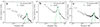 |
Fig. 1. Power density spectrum and QPO analysis results. Panels a–c display the PDS in black and the HHT decomposed QPO in green from (a) a single NICER observation, (b) combined NICER observation data, and (c) a single NuSTAR observation. The prominent peak at 0.2 Hz in these panels confirms the stability of the QPO signal for different observations. |
3.2. Spectral analysis
The single spectrum from NuSTAR was used to constrain the broadband spectral shape in the combined spectra, and combined NICER data were used to focus on the spectral properties. Based on Fig. 11 in Kong et al. (2024), we assumed that combining the spectra is reasonable because the shape of the spectra remains stable over the period of the 20 observations, with a photon index Γ around 3.5 and kTbb around 1.1 keV, except for the drop at the beginning. On the other hand, the absorption properties are also stable, with nH around 40 and the log ξ around 4.
Following Kong et al. (2024), we considered the disk in the rebrightening event, which might extend far beyond the standard thin disk and be encased in a warm layer (Zhang et al. 2000; Gronkiewicz & Różańska 2020). This warm layer is stronger for higher accretion rates and greater magnetic field strengths (Gronkiewicz & Różańska 2020). Following Zhang et al. (2000), Pszota & Cui (2007), we replaced diskbb to comptt to model the disk emission with saturated Compton scattering (Titarchuk 1994). The kT0 value for the comptt model was linked to kT/2.7fcol during the fitting, where the color factor fcol = 1.7, representing a standard disk (see Pszota & Cui 2007 for more details). From model 2 in Table 1 of Kong et al. (2024), the optical depth of the compttτ0 is higher than 50. This means that the seed photons with a temperature kT ≃ 1 keV that escape the warm layer as blackbody emission can be Comptonized to higher energies as they pass through the corona. Therefore, we used the thermally Comptonized model thcomp (Zdziarski et al. 2020) convolved with comptt to fit the continuum. The absorption by the interstellar medium (ISM) was accounted for using the Tuebingen-Boulder ISM absorption model TBabs, with abundances as in Wilms et al. (2000), and with the photoelectric cross sections given in Verner et al. (1996). The equivalent hydrogen column density nH was fixed at 4.9 based on the results from Kong et al. (2024). The cross-calibration between NICER and NuSTAR was performed using the Crabcorr(plabs) model rather than a simple constant (Steiner et al. 2010; Wang et al. 2020). This model multiplies each spectrum by a power law with an index and coefficient parameters, and corrections were applied to both the slope and normalization. Because of this, the continuum model can be written as plabs × TBabs × thcomp ⊗ comptt. This approach allowed us to account for the energy-dependent response differences between the detectors and to normalize the data to the Crab nebula, ensuring a consistent calibration across the different instruments. Specifically, the model adjusts for the known slope differences between the NICER and NuSTAR energy ranges and aligns the spectra to a common reference. This is essential because NICER and NuSTAR cover different energy bands and have varying sensitivities.
The fit that only considered the continuum spectrum yielded a large reduced χ2 that left at least seven narrow absorption features below 9 keV and one broad dip around 7−15 keV (see panels c and d in Fig. 2). We used four gabs components to fit the narrow absorption features at approximately 6.7 keV, 6.97 keV, 7.8 keV, and 8.27 keV, which correspond to the Fe XXV He-α, Fe XXVI Ly-α, Fe XXV He-β, and Fe XXVI Ly-β lines, respectively. Although there are some other structures below 4 keV (see Fig. 2), we ignored them because only iron is the most abundant element, which provides a better illustration for the study. The broad dip was fit with an absorption edge at ≃8.7 keV, which resembles the Fe XXV K-edge. Our new model can produce good residuals. Therefore, the fitting model we used for panels (a) in 0.0 − 0.1 QPO phase and (b) in 0.5 − 0.6 QPO phase is represented as plabs × TBabs × (4 × gabs)×edge × thcomp ⊗ comptt. In this model, gabs denotes the absorption lines, and edge refers to the absorption edge. In Table 1, we show the fitting results of the phase average, 0.0 − 0.1, and 0.5 − 0.6 QPO phase. For the phase-resolved analysis, the energy and width of four absorption lines and the optical depth (τ0) of the comptt were fixed during the fitting.
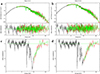 |
Fig. 2. Spectral fitting and residual analysis for NICER and NuSTAR observations. Panels a and b: Spectral fit using the model TBabs × (4 × gabs)×edge × thcomp × comptt. The black lines represent the NICER data in the energy range of 1−10 keV. The red and green lines correspond to the NuSTAR data from the FPMA and FPMB mirrors, respectively, covering the energy range of 4−25 keV. Panels c and d: Residuals of the spectral fit without the gabs and edge components. The black lines indicate the NICER data, and the red and green lines represent the FPMA and FPMB data from NuSTAR. The depicted energy ranges are 2−10 keV for NICER and 10−25 keV for NuSTAR. |
Joint fitting results of NICER (20 combined observations) and NuSTAR.
We combined NICER data to obtain a long-exposure spectral fit. The result is shown in Fig. 2. NuSTAR data cover the energy range of 4−25 keV, ensuring a comprehensive coverage of the spectral features and allowing for a detailed comparison between the NICER and NuSTAR data. Panels c and d focus on the residuals without gabs and edge from the fittings. This is shown for the energy range of 2−25 keV. We deliberately excluded the NuSTAR data below 10 keV when we plotted the residuals for clarity. The residuals are better visible, and this allows a clearer assessment of the model performance with the NICER data.
Figure 3 presents the results of the QPO phase-resolved spectral fitting analysis. The QPO phase obtained from NICER data in 1−10 keV and derived from a single NuSTAR observation in 3−79 keV. It shows variations in the iron absorption components and continuum parameters across different QPO phase. Because we focused on the variation in the absorption and because the energy of the lines does not vary with phases, we froze the line energies in accordance with physical scenarios. The four gabs components for the iron lines were fixed to specific energy. Notably, the two absorption lines of Fe XXV vary slightly with QPO phase, as observed from the fitting results. The variation in the absorption edge with the QPO phase is more pronounced. To calculate the significance, we employed a nonlinear least-squares method to fit a sinusoidal model to the data in one period. We took the measurement errors into account. The fitting process involved minimizing the χ2 statistic. Based on an f-test, we compared the fits from the sinusoidal and the constant model. Our calculations and fitting in Fig. 4 show that the p value of the f-test is 2.7 × 10⁻³, and the confidence level of this variation is approximately 3σ, indicating a significant variation. This variation underscores the dynamic nature of the absorption edge in response to the changes in QPO phase.
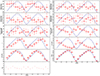 |
Fig. 3. QPO phase derived from combined NICER data (blue line) and a single NuSTAR observation (black line). The first four panels illustrate the strength of the iron absorption lines: Fe XXV He-α at ≃6.7 keV, Fe XXVI Ly-α at ≃6.97 keV, Fe XXV He-β at ≃7.8 keV, and Fe XXVI Ly-β at ≃8.27 keV, each shown with respect to the QPO phase. The fifth and sixth panels in the third row depict the edge threshold energy (edgeE) and absorption depth (MaxTau) of the Fe XXV K-edge. The fourth and fifth rows show the change in the continuum parameters with QPO phase. Finally, the last panel displays the spectral fitting residuals. |
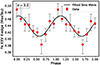 |
Fig. 4. Confidence level of the variation between the absorption depth (MaxTau) of Fe XXV K-edge and the QPO phase (3σ). The black line represents the fitted sine wave based on the simulation results, and the red points indicate the actual observational data, complete with error bars. |
Beyond the variation in the absorption lines and edges, other spectral parameters also change significantly with QPO phase. Specifically, the optical depth τ, the seed photon temperature kT, and the seed photon normalization show a positive correlation with the QPO phase. In contrast, the electron temperature kTe is anticorrelated with the flux of the QPO phase. This highlights the complex interplay between these parameters and the QPO phenomena. To further validate the spectrum fitting results, we constructed a multiparameter correlation diagram (Fig. A.1). This diagram reveals that the absorption K-edge of Fe XXV and the absorption lines are not affected by other parameters. This confirms their independence. However, the parameters of the continuous spectrum are strongly correlated, in particular, between those of the comptt and thcomp models. This strong interparameter correlation emphasizes that when the parameters of the continuum model are discussed, we should be mindful of the competing relation between this correlation trend and their broader tendency to vary with QPO phase.
The spectral fitting results in Fig. 3 delineate the modulation patterns of various spectral features with QPO phase and provide a strong statistical significance about the Fe XXV K-edge absorption component. The correlation analysis further corroborates the independence and interdependence of key spectral parameters, which ensures that the modulation results with QPO phase are reliable.
4. Discussions
Our spectral fitting results, in conjunction with previous findings in Kong et al. (2024), provide significant insights into the nature of the X-ray emissions and their variation with QPO phase. The soft X-ray rebrightening observed in 2021 suggests that the radiation predominantly stems from Compton-thick (τ ≃ 5.5) low-temperature electrons (kTe ≃ 3.5 keV) in the corona, with the seed photons (kT ≃ 1.06 keV) arising from the disk emission, diluted by the optically thick warm layer, accompanied by a QPO signal that is characterized by high column densities and a wind with a high ionization degree.
For the canonical low-mass black hole binaries (LMBHs), the occurrence of type-C low-frequency QPOs (LFQPOs) at ≃0.2 Hz is more prevalent in hard states than in the soft state (Motta et al. 2011), and the frequency of the LFQPOs is positively correlated to the photon index (Vignarca et al. 2003). In addition, in combination with the tendency of QPO properties to vary with inclination angle, coronal or jet precession models are currently preferred to explain the origin of QPOs (Ingram et al. 2016; Ma et al. 2021). However, (Kong et al. 2024) posited that the establishment and elimination of these QPOs largely depends not on the evolution of the spectral shape, such as the photon index and the electron temperature, but on the properties of the disk wind, including the ionization degree and the column density. Our results show a positive correlation between the optical depth τ and the QPO flux, however, which is opposite to the behavior observed in H1743−322, MAXI J1820+070, and Swift J1727.8−1613, where an anticorrelation (or a positive correlation between the photon index Γ and the QPO flux) was observed (Ingram et al. 2016; Shui et al. 2023). More importantly, we have discovered for the first time that the wind properties vary with QPO phase. We would like to emphasize that this observation contradicts models that rely on coronal precession to explain the observed phenomena, because the disk wind is always generated on the disk and is produced farther away from the black hole, regardless of the driving mechanism. This makes the Lense-Thirring precession weak. The highly ionized winds that accompany LFQPOs imply that the energy of the black hole activity is injected into the wind through quasi-periodic dynamical processes, which cause it to be heated. This behavior of the energy transfer also occurs in the usual QPO phenomena of GRS 1915+105, such as in the transformation into the relativistic jet or the accreting corona (Méndez et al. 2022). However, the sudden drop in the radio flux during the rebrightening is evidence of suppressed jet activity (Sánchez-Sierras et al. 2023), which implies that energy can only be fed into the Compton-thick low-temperature corona or into the highly ionized wind. The established facts above demonstrate that the LFQPO that was observed during the rebrightening is distinctly different from the usual LFQPO phenomenon in GRS 1915+105.
In Fig. 3, the positive correlation of the optical depth τ, the seed photon temperature kT, and the normalization factor with QPO phase is reasonable. When we generally accept that the flux of photons is determined by the optical depth and the normalization of the seed photon, which controls the Comptonization, then the high QPO intensity implies a relatively high optical depth τ and norm (see Fig. 3). This increases the scattering times, however, and results in lower electron temperatures, which is also consistent with a colder and larger corona. Our results also indicate that the strength of the iron absorption is anticorrelated with the QPO flux. This suggests that fewer materials are ejected as wind during a high QPO flux, but they instead cool and fall back to the corona, leading to a thicker corona with a higher optical depth and a thinner wind with a weaker absorption strength, as indicated by the continuum spectral fit parameters. Consequently, the increase in the thickness of the absorbing wind occurs simultaneously with the contraction of the corona scale, or vice versa. This interpretation was obtained from the results of our energy spectrum fit. This suggests that there might be other plausible explanations. During the rebrightening phase, the energies of the absorption lines do not show a significant mismatch (see Table 1). This indicates minimal red- and blueshifts. Without considering limitations from the detector resolution, we suggest based on the low-velocity winds that the driving force creates a dynamic equilibrium with gravitational forces, resulting in failed winds (Miller et al. 2020). In this case, we assume that the energy injection that carries the oscillatory signal can be retained in the failed wind, which causes the variation. Because the change with QPO phase occurs on short timescales, we speculate that this type of variation is highly likely to be related to magnetic processes.
These phenomena can be explained by the accretion ejection instability (AEI) model (Tagger & Pellat 1999), which attributes them to processes driven by the magnetic field, which play an important role in generating both QPOs and ejections, such as wind (Kong et al. 2024). The AEI model offers a plausible explanation for the change in the iron absorption lines and in the continuum spectrum with QPO phase. This model posits that the instabilities in the inner regions of the accretion disk, where magnetic field lines are twisted and sheared, can drive periodic ejections of material from the disk. This is observed as QPOs. When the magnetic field on the disk is strong enough, the magnetic pressure created by these twisted field lines, combined with differential rotation, launches material from the disk surface into a wind. Based on the comprehensive analysis and the robust statistical significance of our findings, it is evident that the observed modulations are consistent with the predictions of the AEI model. This model not only explains the occurrence of low-frequency QPOs in soft states, but also accounts for the variation in the iron absorption lines and continuum spectral parameters with QPO phase. Furthermore, our results suggest that the potential conversion of the corona into disk winds during magnetism-driven processes is a plausible scenario that indicates a complex interplay between these components.
Figure 5 presents a schematic that illustrates the transformation of the corona into wind during a QPO phase. The accretion disk is far from the black hole and is overlaid by the inner corona layer and the outer wind layer, which are both influenced by magnetic fields. During a QPO phase with high flux (upper panel in Fig. 5), the size of corona is largest, as indicated by the dashed red line. As the flux decreases, the corona scale shrinks, resulting in an increase in ejected material, which is further converted into disk wind. Our results in Fig. 3 show significant change in the spectral features with QPO phase. In the interface area (the dashed lines shown in Fig. 5), the contraction (dashed blue line) and expansion (dashed red line) of the corona during different QPO phases indicates a dynamic interaction between the magnetic fields and the ionized gas that results in the periodic ejection of material from the corona into the wind and the cooling of material from the wind back to the corona. Furthermore, we note that the nature of the disk during this event may extend beyond the simple geometric thin disk. It might be enveloped in a warm layer that is stronger in cases of higher accretion rates and greater magnetic field strengths (Zhang et al. 2000; Gronkiewicz & Różańska 2020). This is self-consistent with the assumption of a strong magnetic field in the model.
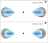 |
Fig. 5. Simplified schematic diagram of the transformation from the corona (blue area) to the wind (gray area) during the QPO phases. We show the change in a region of gas with a hot electron above the disk, referred to as the corona, in response to QPO phases. The diagram shows that the variation in the corona is anticorrelated with the ejection of ionized material through the disk wind during different QPO phases. The top and bottom panels show the situations of the QPO peak at 0.5−0.6 phase and the QPO trough at 0.0−0.1 phase. The dashed red and blue lines indicate the corona size at the highest and lowest points of the QPO phase, respectively. |
Because this QPO phenomenon has not been captured in large numbers and in more sources, and considering the unique nature of GRS 1915+105 during its reflare process as well as the limited observational data available during this period, additional explanations are possible. These limitations may allow room for different interpretations of the observed phenomena. We expect that subsequent larger samples of observations as well as more observed polarization events will make it possible to constrain the model better. The capabilities of the future enhanced X-ray Timing and Polarimetry mission (eXTP) will provide huge advantages for these observations (Zhang et al. 2019). Our findings underscore overall the new intricate relation between QPOs, disk winds, and the magnetic dynamics within the accretion process of the black hole binary system. This contributes to a deeper understanding of the physical processes driving these phenomena.
5. Conclusions
This study has provided a comprehensive analysis of the spectral fitting results from NICER and NuSTAR observations of the X-ray source GRS 1915+105, with a focus on the variation in the spectral features with QPO phase. Our findings revealed significant variation in the iron absorption lines and edge with QPO phase, indicating dynamic changes in the source environment. The strong variation in the iron absorption edge that we reported with high confidence highlights substantial physical variations in the wind near the source during different QPO phases. We also observed that the continuum spectral parameters are (anti-)correlated with the QPO phase. These findings agree better with the AEI model than with the geometric precession model. The former attributes the QPO generation to instabilities in the inner accretion disk, caused by twisted magnetic fields, which naturally give rise to a periodically varying magnetically driven disk wind. Additionally, the disk nature during this event may involve a warm layer. This would affect the radiation dilution and provide further context for the magnetic accretion disk structure in GRS 1915+105.
In summary, this study advances our understanding of QPOs and the related radiation dynamics by revealing the intricate interplay between disk winds, magnetic fields, and the corona. Future research should extend these findings to other QPO sources and refine the theoretical models for a deeper understanding of these dynamic systems.
Acknowledgments
This work made use of data from the the High Energy Astrophysics Science Archive Research Center (HEASARC), provided by NASA’s Goddard Space Flight Center. Xiaohang Dai is grateful for the financial supported provided by the China Scholarship Council (CSC) at Eberhard Karls Universität of Tübingen. Lingda Kong is grateful for the financial support provided by the Sino-German (CSC-DAAD) Postdoc Scholarship Program (57607866).
References
- Arnaud, K. A. 1996, ASP Conf. Ser., 101, 17 [Google Scholar]
- Athulya, M. P., & Nandi, A. 2023, MNRAS, 525, 489 [NASA ADS] [CrossRef] [Google Scholar]
- Belloni, T., Klein-Wolt, M., Méndez, M., van der Klis, M., & van Paradijs, J. 2000, A&A, 355, 271 [Google Scholar]
- Cabanac, C., Henri, G., Petrucci, P. O., et al. 2010, MNRAS, 404, 738 [NASA ADS] [CrossRef] [Google Scholar]
- Carvalho, V. R., Moraes, M. F., Braga, A. P., & Mendes, E. M. 2020, Biomed. Signal Process. Control, 62, 102073 [CrossRef] [Google Scholar]
- Castro-Tirado, A. J., Brandt, S., & Lund, N. 1992, IAU Circ., 5590, 2 [NASA ADS] [Google Scholar]
- Done, C., Gierliński, M., & Kubota, A. 2007, A&ARv, 15, 1 [Google Scholar]
- Dragomiretskiy, K., & Zosso, D. 2014, IEEE Trans. Signal Process., 62, 531 [CrossRef] [Google Scholar]
- Fender, R., & Belloni, T. 2004, ARA&A, 42, 317 [NASA ADS] [CrossRef] [Google Scholar]
- Fender, R. P., & Belloni, T. M. 2012, Science, 337, 540 [NASA ADS] [CrossRef] [Google Scholar]
- Fuchs, Y., Rodriguez, J., Mirabel, I. F., et al. 2003, A&A, 409, L35 [NASA ADS] [CrossRef] [EDP Sciences] [Google Scholar]
- Gendreau, K. C., Arzoumanian, Z., Adkins, P. W., et al. 2016, SPIE Conf. Ser., 9905, 99051H [NASA ADS] [Google Scholar]
- Gronkiewicz, D., & Różańska, A. 2020, A&A, 633, A35 [NASA ADS] [CrossRef] [EDP Sciences] [Google Scholar]
- Harrison, F. A., Craig, W. W., Christensen, F. E., et al. 2013, ApJ, 770, 103 [Google Scholar]
- Huang, N. E., & Wu, Z. 2008, Rev. Geophys., 46, RG2006 [CrossRef] [Google Scholar]
- Huang, N. E., Shen, Z., Long, S. R., et al. 1998, Proc. Roy. Soc. London Ser. A, 454, 903 [NASA ADS] [CrossRef] [Google Scholar]
- Huang, Y., Qu, J. L., Zhang, S. N., et al. 2018, ApJ, 866, 122 [NASA ADS] [CrossRef] [Google Scholar]
- Huppenkothen, D., Bachetti, M., Stevens, A. L., et al. 2019a, ApJ, 881, 39 [Google Scholar]
- Huppenkothen, D., Bachetti, M., Stevens, A., et al. 2019b, J. Open Source Softw., 4, 1393 [NASA ADS] [CrossRef] [Google Scholar]
- Ingram, A., van der Klis, M., Middleton, M., et al. 2016, MNRAS, 461, 1967 [NASA ADS] [CrossRef] [Google Scholar]
- Kaastra, J. S., & Bleeker, J. A. M. 2016, A&A, 587, A151 [NASA ADS] [CrossRef] [EDP Sciences] [Google Scholar]
- Klein-Wolt, M., Fender, R. P., Pooley, G. G., et al. 2002, MNRAS, 331, 745 [Google Scholar]
- Koljonen, K. I. I., & Hovatta, T. 2021, A&A, 647, A173 [NASA ADS] [CrossRef] [EDP Sciences] [Google Scholar]
- Koljonen, K. I. I., & Tomsick, J. A. 2020, A&A, 639, A13 [EDP Sciences] [Google Scholar]
- Kong, L. D., Zhang, S., Chen, Y. P., et al. 2020, J. High Energy Astrophys., 25, 29 [NASA ADS] [CrossRef] [Google Scholar]
- Kong, L.-D., Ji, L., Santangelo, A., et al. 2024, A&A, 686, A211 [NASA ADS] [CrossRef] [EDP Sciences] [Google Scholar]
- Lee, J. C., Reynolds, C. S., Remillard, R., et al. 2002, ApJ, 567, 1102 [NASA ADS] [CrossRef] [Google Scholar]
- Ma, X., Tao, L., Zhang, S.-N., et al. 2021, Nat. Astron., 5, 94 [NASA ADS] [CrossRef] [Google Scholar]
- Majumder, S., Sreehari, H., Aftab, N., et al. 2022, MNRAS, 512, 2508 [NASA ADS] [CrossRef] [Google Scholar]
- Méndez, M., Karpouzas, K., García, F., et al. 2022, Nat. Astron., 6, 577 [CrossRef] [Google Scholar]
- Miller, J. M., Raymond, J., Fabian, A., et al. 2006, Nature, 441, 953 [NASA ADS] [CrossRef] [Google Scholar]
- Miller, J. M., Zoghbi, A., Raymond, J., et al. 2020, ApJ, 904, 30 [Google Scholar]
- Mirabel, I. F., & Rodríguez, L. F. 1999, ARA&A, 37, 409 [Google Scholar]
- Morgan, E. H., Remillard, R. A., & Greiner, J. 1997, ApJ, 482, 993 [NASA ADS] [CrossRef] [Google Scholar]
- Motta, S. E., & Belloni, T. M. 2024, A&A, 684, A209 [NASA ADS] [CrossRef] [EDP Sciences] [Google Scholar]
- Motta, S., Muñoz-Darias, T., Casella, P., Belloni, T., & Homan, J. 2011, MNRAS, 418, 2292 [NASA ADS] [CrossRef] [Google Scholar]
- Motta, S. E., Casella, P., Henze, M., et al. 2015, MNRAS, 447, 2059 [NASA ADS] [CrossRef] [Google Scholar]
- Motta, S. E., Kajava, J. J. E., Giustini, M., et al. 2021, MNRAS, 503, 152 [Google Scholar]
- Neilsen, J., & Lee, J. C. 2009, Nature, 458, 481 [NASA ADS] [CrossRef] [Google Scholar]
- Neilsen, J., Altamirano, D., Homan, J., et al. 2021, ATel, 14792, 1 [NASA ADS] [Google Scholar]
- Ponti, G., Fender, R. P., Begelman, M. C., et al. 2012, MNRAS, 422, L11 [NASA ADS] [CrossRef] [Google Scholar]
- Pszota, G., & Cui, W. 2007, ApJ, 663, 1201 [CrossRef] [Google Scholar]
- Ravishankar, B. T., Tilak, K., Athulya, M. P., et al. 2021, ATel, 14811, 1 [NASA ADS] [Google Scholar]
- Remillard, R. A., & McClintock, J. E. 2006, ARA&A, 44, 49 [Google Scholar]
- Rodriguez, J., Shaw, S. E., Hannikainen, D. C., et al. 2008, ApJ, 675, 1449 [NASA ADS] [CrossRef] [Google Scholar]
- Sánchez-Sierras, J., Muñoz-Darias, T., Motta, S. E., et al. 2023, A&A, 680, L16 [NASA ADS] [CrossRef] [EDP Sciences] [Google Scholar]
- Shui, Q. C., Zhang, S., Zhang, S. N., et al. 2023, ApJ, 957, 84 [NASA ADS] [CrossRef] [Google Scholar]
- Shui, Q. C., Zhang, S., Zhang, S. N., et al. 2024, ApJ, 965, L7 [NASA ADS] [CrossRef] [Google Scholar]
- Steiner, J. F., McClintock, J. E., Remillard, R. A., et al. 2010, ApJ, 718, L117 [Google Scholar]
- Stella, L., & Angelini, L. 1992, Data Anal. Astron., 59 [Google Scholar]
- Tagger, M., & Pellat, R. 1999, A&A, 349, 1003 [NASA ADS] [Google Scholar]
- Taylor, J. E. 2003, MNRAS, 341, 823 [NASA ADS] [CrossRef] [Google Scholar]
- Titarchuk, L. 1994, ApJ, 434, 570 [NASA ADS] [CrossRef] [Google Scholar]
- Titarchuk, L., & Fiorito, R. 2004, ApJ, 612, 988 [NASA ADS] [CrossRef] [Google Scholar]
- Ueda, Y., Yamaoka, K., & Remillard, R. 2009, ApJ, 695, 888 [NASA ADS] [CrossRef] [Google Scholar]
- Varnière, P., & Blackman, E. G. 2005, New Astron., 11, 43 [CrossRef] [Google Scholar]
- Varnière, P., & Tagger, M. 2002, A&A, 394, 329 [NASA ADS] [CrossRef] [EDP Sciences] [Google Scholar]
- Varnière, P., Tagger, M., & Rodriguez, J. 2012, A&A, 545, A40 [NASA ADS] [CrossRef] [EDP Sciences] [Google Scholar]
- Verner, D. A., Ferland, G. J., Korista, K. T., & Yakovlev, D. G. 1996, ApJ, 465, 487 [Google Scholar]
- Vignarca, F., Migliari, S., Belloni, T., Psaltis, D., & van der Klis, M. 2003, A&A, 397, 729 [NASA ADS] [CrossRef] [EDP Sciences] [Google Scholar]
- Wang, J., Kara, E., Steiner, J. F., et al. 2020, ApJ, 899, 44 [NASA ADS] [CrossRef] [Google Scholar]
- Wilms, J., Allen, A., & McCray, R. 2000, ApJ, 542, 914 [Google Scholar]
- Zdziarski, A. A., Szanecki, M., Poutanen, J., Gierliński, M., & Biernacki, P. 2020, MNRAS, 492, 5234 [NASA ADS] [CrossRef] [Google Scholar]
- Zhang, S. N., Cui, W., Chen, W., et al. 2000, Science, 287, 1239 [Google Scholar]
- Zhang, S., Santangelo, A., Feroci, M., et al. 2019, Sci. China Phys. Mech. Astron., 62, 29502 [Google Scholar]
- Zhang, L., Méndez, M., Altamirano, D., et al. 2020, MNRAS, 494, 1375 [Google Scholar]
Appendix A: Parameter correction
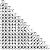 |
Fig. A.1. Distribution of the parameters from the 100,000 chain of MCMC results of the spectral fittings on the QPO phase 0.5-0.6 (for visualization purposes). The multi-parameter correlations indicate that only the continuum parameters, kTe and τ from the thcomp, and kT and Norm from the comptt components exhibit strong correlations. In contrast, the strength of the absorption lines and edge show no significant correlation with other parameters. |
Appendix B: HHT functions
The VMD process involves solving a constrained optimization problem. Firstly, a single-sided band analytic signal is constructed:
![$$ \begin{aligned} s_k(t) = \left[ \delta (t) + \frac{j}{\pi t} \right] * u_k(t), \end{aligned} $$](/articles/aa/full_html/2024/12/aa52132-24/aa52132-24-eq55.gif)
where δ(t) is the Dirac delta function, uk(t) is the k-th mode, and denotes convolution. Each mode’s spectrum is shifted to the baseband by complex modulation:

where ωk is the center frequency of the k-th mode. Finally, the bandwidth of each mode is minimized:
![$$ \begin{aligned} \min _{\{u_k\}, \{\omega _k\}} \left\{ \sum _{k = 1}^{K} \left\Vert \partial _t \left[\left(\delta (t) + \frac{j}{\pi t}\right) * u_k(t) \right] e^{-j \omega _k t} \right\Vert_2^2 \right\} , \end{aligned} $$](/articles/aa/full_html/2024/12/aa52132-24/aa52132-24-eq57.gif)
where ∂t denotes the time derivative. By introducing a quadratic penalty term and Lagrange multipliers, this constrained optimization problem is converted into an unconstrained problem:
![$$ \begin{aligned} L(u_k, \omega _k, \lambda ) = \alpha \sum _{k = 1}^{K} \left\Vert \partial _t \left[\left( \delta (t) + \frac{j}{\pi t} \right) * u_k(t) \right] e^{-j \omega _k t} \right\Vert_2^2 + \left\Vert f(t) - \sum _{k = 1}^{K} u_k(t) \right\Vert_2^2 + \left\langle \lambda (t), f(t) - \sum _{k = 1}^{K} u_k(t) \right\rangle , \end{aligned} $$](/articles/aa/full_html/2024/12/aa52132-24/aa52132-24-eq58.gif)
where λ is the Lagrange multiplier, f(t) is the original signal, and α controls the bandwidth of each mode. Solving this Lagrangian problem using the alternating direction method of multipliers, we can obtain each mode and their center frequencies. α and K are two parameters that need to be considered for introduction. Here, we determine them manually by matching the QPO component of the IMF to the shape of the power spectrum (see Fig. 1). In our analysis, the bandwidth of each mode is controlled by a parameter α, which we set to 100. We chose to decompose the signal into 3 modes (K = 3), capturing the QPO characteristics effectively (see Fig. 1). A larger α above 500 and K above 3 will cause the narrow QPO component (the second IMF) and the band-limited noise (the first IMF) to mismatch with the PDS. After obtaining the IMFs using VMD, we applied the Hilbert transform to each IMF to compute the instantaneous frequency:
![$$ \begin{aligned} H[IMF_i(t)] = \frac{1}{\pi } P \int \frac{IMF_i(\tau )}{t - \tau } d\tau , \end{aligned} $$](/articles/aa/full_html/2024/12/aa52132-24/aa52132-24-eq59.gif)
where P denotes the Cauchy principal value. The analytic signal is then constructed as
![$$ \begin{aligned} z_i(t) = IMF_i(t) + jH[IMF_i(t)] = a_i(t)e^{j\theta _i(t)}, \end{aligned} $$](/articles/aa/full_html/2024/12/aa52132-24/aa52132-24-eq60.gif)
where ai(t) is the instantaneous amplitude, and θi(t) is the instantaneous phase. The instantaneous frequency is given by
Appendix C: Simulation analysis
To ensure the reliability and validity of the QPO phase-folding analysis results, we conducted a comprehensive simulation analysis to test the robustness of our HHT-based method. Our simulation follows these steps (Shui et al. 2024): (1) Fit the PDS of real observations with a multi-Lorentz line profile; (2) Use the fitting parameters of the QPO and noise components to simulate total light curves, which are the sum of the QPO light curve and noise light curve, based on the Python package Stingray.simulator (Huppenkothen et al. 2019a; 3) Test the ability of the VMD algorithm to decompose the signal into QPO and low-frequency noise components accurately by comparing the simulated signals with the HHT-decomposed signals.
We select the original signal and use powspec to generate the PDS. The total model is plotted as a green line in the right panel of Fig. C.1. The parameters of the QPO are fQPO = 0.178 Hz, FWHMQPO = 0.047 Hz and RMSQPO = 0.077. The parameters of the low-break-frequency noise are fN1 = 0 Hz, FWHMN1 = 0.021 Hz and RMSN1 = 0.005. The parameters of the high-break-frequency noise are fN2 = 0 Hz, FWHMN2 = 0.74 Hz and RMSN1 = 0.0149. The simulations of the light curves were performed using Stingray.simulator. The total light curve, with an average count rate of 249 cts/s, includes both red noise and the QPO, and is shown as black points in the left panel of Fig. C.1. The PDS of the simulated light curve is plotted as black points in the right panel of Fig. C.1, while the gray points represent the QPO and noise components in the PDS from the simulation. We find that these components fit the original PDS well.
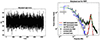 |
Fig. C.1. Simulated light curve and power density spectrum (PDS) analysis. Left panel: Simulated light curve with two broadband noise components at different break frequencies and one QPO signal at ∼0.18 Hz. Right panel: PDS of the simulated light curve (black points) and the fitting model of the real PDS (green line). The gray lines represent the simulated low-frequency noise and QPO components in the PDS. The blue and red lines represent the VMD components of noise and the QPO signal in the PDS. |
After obtaining the simulated data, we performed the VMD-HHT analysis. The IMF components from the VMD of the simulated light curve are shown in Fig. C.2. The blue line and red line represent the low-frequency noise and QPO, respectively. The PDS of these two components is plotted as blue and red lines in the right panel of Fig. C.1. The VMD components show good alignment with the simulated components. In Fig. C.3, we assess the reliability of this method by showing the correlations between the simulated results and the decomposed results, including the QPO count rate and QPO phases in the top panels. The bottom panels show histograms of the count rate difference and phase difference between the simulated QPO and decomposed QPO signals, respectively. The red dashed lines in both the top and bottom panels represent perfect alignment between the two signals. We find that the structure of the decomposed QPO is highly consistent with that of the simulated QPO signal, though with local fluctuations, possibly due to mode mixing between the QPO and noise components, or statistical fluctuations. Specifically, in the right top panel of Fig. C.3, a small number of data points are distributed in the upper left and lower right of the plot, corresponding to the phase difference distributed around −2π and 2π in the right bottom panel. Since the QPO phase varies from −π and −π, this phenomenon reflects local phase shifts between the simulated and decomposed QPO signals in a small portion of time bins.
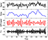 |
Fig. C.2. IMFs obtained from the VMD of the simulated light curve. The blue and red lines represent the low-frequency noise and QPO signals, respectively. |
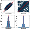 |
Fig. C.3. Comparison between simulated and decomposed QPO signals. Top panels: Correlations between the simulated results and decomposed results, including the QPO count rate and QPO phases. Bottom panels: Histograms of the count rate difference and phase difference between the simulated QPO and decomposed QPO signals. The dashed red lines in both the top and bottom panels represent the case where the two signals are in perfect alignment. |
All Tables
All Figures
|
Fig. 1. Power density spectrum and QPO analysis results. Panels a–c display the PDS in black and the HHT decomposed QPO in green from (a) a single NICER observation, (b) combined NICER observation data, and (c) a single NuSTAR observation. The prominent peak at 0.2 Hz in these panels confirms the stability of the QPO signal for different observations. |
| In the text | |
|
Fig. 2. Spectral fitting and residual analysis for NICER and NuSTAR observations. Panels a and b: Spectral fit using the model TBabs × (4 × gabs)×edge × thcomp × comptt. The black lines represent the NICER data in the energy range of 1−10 keV. The red and green lines correspond to the NuSTAR data from the FPMA and FPMB mirrors, respectively, covering the energy range of 4−25 keV. Panels c and d: Residuals of the spectral fit without the gabs and edge components. The black lines indicate the NICER data, and the red and green lines represent the FPMA and FPMB data from NuSTAR. The depicted energy ranges are 2−10 keV for NICER and 10−25 keV for NuSTAR. |
| In the text | |
|
Fig. 3. QPO phase derived from combined NICER data (blue line) and a single NuSTAR observation (black line). The first four panels illustrate the strength of the iron absorption lines: Fe XXV He-α at ≃6.7 keV, Fe XXVI Ly-α at ≃6.97 keV, Fe XXV He-β at ≃7.8 keV, and Fe XXVI Ly-β at ≃8.27 keV, each shown with respect to the QPO phase. The fifth and sixth panels in the third row depict the edge threshold energy (edgeE) and absorption depth (MaxTau) of the Fe XXV K-edge. The fourth and fifth rows show the change in the continuum parameters with QPO phase. Finally, the last panel displays the spectral fitting residuals. |
| In the text | |
|
Fig. 4. Confidence level of the variation between the absorption depth (MaxTau) of Fe XXV K-edge and the QPO phase (3σ). The black line represents the fitted sine wave based on the simulation results, and the red points indicate the actual observational data, complete with error bars. |
| In the text | |
|
Fig. 5. Simplified schematic diagram of the transformation from the corona (blue area) to the wind (gray area) during the QPO phases. We show the change in a region of gas with a hot electron above the disk, referred to as the corona, in response to QPO phases. The diagram shows that the variation in the corona is anticorrelated with the ejection of ionized material through the disk wind during different QPO phases. The top and bottom panels show the situations of the QPO peak at 0.5−0.6 phase and the QPO trough at 0.0−0.1 phase. The dashed red and blue lines indicate the corona size at the highest and lowest points of the QPO phase, respectively. |
| In the text | |
|
Fig. A.1. Distribution of the parameters from the 100,000 chain of MCMC results of the spectral fittings on the QPO phase 0.5-0.6 (for visualization purposes). The multi-parameter correlations indicate that only the continuum parameters, kTe and τ from the thcomp, and kT and Norm from the comptt components exhibit strong correlations. In contrast, the strength of the absorption lines and edge show no significant correlation with other parameters. |
| In the text | |
|
Fig. C.1. Simulated light curve and power density spectrum (PDS) analysis. Left panel: Simulated light curve with two broadband noise components at different break frequencies and one QPO signal at ∼0.18 Hz. Right panel: PDS of the simulated light curve (black points) and the fitting model of the real PDS (green line). The gray lines represent the simulated low-frequency noise and QPO components in the PDS. The blue and red lines represent the VMD components of noise and the QPO signal in the PDS. |
| In the text | |
|
Fig. C.2. IMFs obtained from the VMD of the simulated light curve. The blue and red lines represent the low-frequency noise and QPO signals, respectively. |
| In the text | |
|
Fig. C.3. Comparison between simulated and decomposed QPO signals. Top panels: Correlations between the simulated results and decomposed results, including the QPO count rate and QPO phases. Bottom panels: Histograms of the count rate difference and phase difference between the simulated QPO and decomposed QPO signals. The dashed red lines in both the top and bottom panels represent the case where the two signals are in perfect alignment. |
| In the text | |
Current usage metrics show cumulative count of Article Views (full-text article views including HTML views, PDF and ePub downloads, according to the available data) and Abstracts Views on Vision4Press platform.
Data correspond to usage on the plateform after 2015. The current usage metrics is available 48-96 hours after online publication and is updated daily on week days.
Initial download of the metrics may take a while.