| Issue |
A&A
Volume 686, June 2024
|
|
|---|---|---|
| Article Number | A211 | |
| Number of page(s) | 12 | |
| Section | Astrophysical processes | |
| DOI | https://doi.org/10.1051/0004-6361/202348512 | |
| Published online | 12 June 2024 | |
Likely detection of magnetic field related LFQPO in the soft X-ray rebrightening of GRS 1915+105
1
Institut für Astronomie und Astrophysik, Kepler Center for Astro and Particle Physics, Eberhard Karls, Universität, Sand 1, 72076 Tübingen, Germany
e-mail: This email address is being protected from spambots. You need JavaScript enabled to view it.
2
School of Physics and Astronomy, Sun Yat-Sen University, Zhuhai 519082, PR China
e-mail: This email address is being protected from spambots. You need JavaScript enabled to view it.
3
Key Laboratory for Particle Astrophysics, Institute of High Energy Physics, Chinese Academy of Sciences, 19B Yuquan Road, Beijing 100049, PR China
4
University of Chinese Academy of Sciences, Chinese Academy of Sciences, Beijing 100049, PR China
Received:
6
November
2023
Accepted:
12
March
2024
Abstract
Utilizing NICER observations, we present an analysis of the soft X-ray rebrightening event of GRS 1915+105 observed in 2021. During this event, we observed the emergence of a stable long-lasting low-frequency quasi-periodic oscillation (LFQPO) with frequencies ranging from 0.17 to 0.21 Hz. Through a careful spectral analysis, we demonstrate that a low-temperature Compton-thick gas model characterizes the emitted radiation well. By examining the spectrum and identifying numerous absorption lines, we discerned a transition in the wind properties. This transition was marked by a shift from a state characterized by low speed, high column density, and high ionization degree to one featuring still low speed, but low column density and ionization degree. Intriguingly, the presence or absence of the QPO signal is perfectly correlated with these distinct wind characteristics. The low-speed wind observed could be indicative of a “failed wind”, while the observed shift implies a transition from a magnetically to a thermally driven wind. Notably, this QPO signal exclusively manifested itself during the magnetically driven phase, suggesting the possibility of a novel perturbation associated with magnetic effects.
Key words: accretion / accretion disks / stars: black holes / stars: magnetic field / X-rays: binaries
© The Authors 2024
 Open Access article, published by EDP Sciences, under the terms of the Creative Commons Attribution License (https://creativecommons.org/licenses/by/4.0), which permits unrestricted use, distribution, and reproduction in any medium, provided the original work is properly cited.
This article is published in open access under the Subscribe to Open model. This email address is being protected from spambots. You need JavaScript enabled to view it. to support open access publication.
1. Introduction
GRS 1915+105, a microquasar discovered in 1992 by the GRANAT/WATCH all-sky monitor (Castro-Tirado et al. 1992), is well known for its remarkable variability. It consists of a 12 M⊙ high-spin black hole (BH) and a K-M III companion star (Greiner et al. 2001; Reid et al. 2014). Since its discovery, GRS 1915+105 has been active for 26 yr and has a long history of being monitored by all major all-sky X-ray telescopes. During this long-term period, its variability has been classified into at least 15 different states with unique timing-spectral properties (Belloni et al. 2000; Klein-Wolt et al. 2002; Hannikainen et al. 2005; Athulya et al. 2022). In 2018, experiencing an exponential decay during MJD 58230−58330 and a linear decay during MJD 58330−58500, the source was at a low flux level (see Koljonen & Tomsick 2020; Koljonen & Hovatta 2021, for details). Still in the radio, IR, and X-ray bands, significant variability was observed (Murata et al. 2019; Trushkin et al. 2019a,b, 2020; Koljonen et al. 2019; Vishal et al. 2019; Motta et al. 2021; Egron et al. 2023; Sanchez-Sierras et al. 2023). GRS 1915+105 seems to have transitioned from a canonical hard state to an unusual accretion phase characterized by heavy X-ray absorption and obscuration. The presence of a Compton-thick “failed wind” (Miller et al. 2020; Balakrishnan et al. 2021), which hides from the observer the accretion processes feeding the variable jet responsible for the radio flaring, has been discussed (Motta et al. 2021). This kind of obstruction may be unstable, allowing the internal accretion processes and jets to be briefly observed. In addition, the long-term low X-ray level is always interrupted by short X-ray flares with synchronized radio flares within a few hundred seconds (Trushkin et al. 2019a, 2023; Homan et al. 2019; Neilsen et al. 2020; Kong et al. 2021; Egron et al. 2023).
In the case of GRS 1915+105, it has been observed that massive winds are predominantly found in softer states, although not exclusively (Miller et al. 2020; Ratheesh et al. 2021; Neilsen et al. 2020; Kong et al. 2021). During these softer states, strong jet emissions are generally absent or are relatively weak (Ponti et al. 2012; Homan et al. 2016). Neilsen & Lee (2009) proposed that these massive winds significantly influence the disk accretion flow. They could suppress the formation of jets or even completely quench the jet activity in the system. However, in some exceptional cases a rapid transition between the jet and the wind can occur in the heartbeat state (ρ state). As discussed by Neilsen et al. (2011), the jet on smaller scales during a short period with a 10% cycle near the minimum luminosity of the pulse of the heartbeat, and the disk wind at larger scales may lead the fast spectral transitions in different phases. Zoghbi et al. (2016) also found the presence of two wind components with velocities between 500 and 5000 km s−1 and possibly two more with velocities reaching 20 000 km s−1 (∼0.06 c). The alterations in wind speed and absorbed flux necessitate rapid changes in wind geometry and location within the heartbeat cycle.
Such an evolution of the wind features may be associated with a bulge born in the inner disk and moving outward as the instability progresses (Zoghbi et al. 2016). Through a broadband spectral analysis of the X-ray–radio flare, Kong et al. (2021) found a fast transition between jet and magnetically driven wind. All these results imply that GRS 1915+105 can be a laboratory to study the relations among jet, wind, and magnetic fields on the accretion disk.
In July 2021 a soft X-ray rebrightening was monitored by MAXI/GSC, NICER, and AstroSat (Neilsen et al. 2021; Ravishankar et al. 2021), which is the second rebrightening in the low-flux state after 2018. During this rebrightening, Neilsen et al. (2021) found that the spectrum contains over a dozen strong absorption lines from Si, S, Ar, Ca, Fe, and Ni, as well as an emission line consistent with Fe K-alpha. This suggests the presence of an ionized absorber with Nh > 5 × 1023 cm−2 without evidence of cold Compton-thick obscuration. Meanwhile, as the intensity increased, they found a low-frequency quasi-periodic oscillation (LFQPO) at 0.17 Hz. In black hole binary systems (BHXRBs), LFQPOs typically occur in the low hard state (LHS) and the high intermediate state (HIMS), while the disk wind is commonly observed in the high soft state (HSS). In this soft X-ray rebrightening, the simultaneous presence of both multiple absorption lines (wind feature) and LFQPOs is a truly rare and intriguing event. Through such observations, we can further investigate the nature of disk winds and the origin of LFQPOs.
In this article we focus on an analysis of the evolution of spectral and timing variations through the long-lasting soft X-ray rebrightening of 2021. We also focus on the physical properties and origin of the absorber and LFQPOs. We introduce the data reduction and analysis in Sect. 2 and present the results in Sect. 3. Finally, we present our discussion in Sect. 4, and our conclusions in Sect. 5.
2. Observations and data reduction
The NICER X-ray Timing Instrument (XTI) comprises an array of 56 co-aligned concentrator X-ray optics that are paired with a single-pixel silicon drift detector working in the 0.2–12 keV band (Gendreau et al. 2016). NICER’s energy and time resolutions are 85 eV at 1 keV and 40 ns, respectively.
For this work we used NICER observations between June 17, 2021 (MJD 59382), and October 3, 2021 (MJD 59490), performed during the soft X-ray rebrightening of the source. Due to the occasional increase in the electronic noise, detectors No. 14 and 34 were excluded from the analysis.
NICER is an excellent telescope for observing soft X-rays, due to its effective area of ∼1800 cm2 at 1.5 keV. We used the nicerl2 pipeline task to process each observation by applying the default calibration process and screening. The spectra and light curves were extracted by the nicerl3 pipeline task. The background is calculated with the nibackgen3C50 tool provided by the NICER team. The data analysis was performed under the Heasoft v6.31.1 environment, and NICER’s calibration was updated to October 1, 2022.
For this work we also used the NuSTAR ToO observation started on July 14, 2021, at 06:36:09 (UTC), with a total exposure of 20.44 ks (ObsID: 90701323002). The NuSTAR Data Analysis Software (NuSTARDAS) including nupipeline v0.4.9 and nuproducts with the calibration database version v20230420 was used in this work. We extracted the NuSTAR lightcurves of the source and the background with two circular extraction regions of 100″ and 180″, one centered at the point-like source and another centered away from the source.
All spectra were grouped by ftgrouppha task using the Kaastra & Bleeker (2016) optimal binning scheme with a minimum of 25 counts per bin. Our timing analysis is based on the Python package Stingray (Huppenkothen et al. 2019a,b) and on Xronos 6.0 task powspec (Stella & Angelini 1992). We used Xspec v12.13.0c (Arnaud 1996) to study the spectrum in the frequency and energy domain. We chose the energy range 1 − 10 keV of NICER and 4 − 25 keV of NuSTAR for spectral analysis and took the frequency range 1/128 to 10 Hz for timing analysis. The uncertainties of the spectral parameters were computed using the Markov chain Monte Carlo (MCMC) method with a length of 10 000 and are reported at a 90% confidence level.
3. Data analysis and observational results
In Fig. 1 we present the light curves from the all-sky monitor MAXI in the 2 − 20 keV range and from Swift/BAT in the 15 − 50 keV range after the source enters the low-flux state. In 2020 and 2021 the source experienced two episodes of soft rebrightening, both primarily characterized by an abundance of soft photons. In the top panel of Figs. 2 and 3 we present NICER light curves in the 1 − 4 keV (red points) and 4 − 10 keV (blue points). In the bottom panel we display the dynamic power spectrum (DPS) in the 1 − 10 keV band, which reveals significant variability. Each power density spectrum is computed using Leahy normalization (Leahy et al. 1983), then we subtracted the Poisson noise, which in the case of this normalization levels at 2, to highlight the physical signals (see Figs. 2a and 3a). Due to the long time span of the observation, we removed the gaps between effective observational windows to show the evolution more clearly (see Figs. 2b and 3b). The GTI EXPOSURE (days) means each observation’s net effective exposure time. These time slices are sorted in chronological order of observations. The X-axis in Figs. 2b and 3b shows the total GTI accumulation as time evolves. For the first rebrightening, there is no finding of any LFQPO in 0.1 − 10 Hz, but there are mHz QPOs with ∼20 mHz whose light curves can be classified into the heartbeat state. The primary emphasis of this paper is directed toward the second rebrightening since it shows a more stable LFQPO (at ∼0.2 Hz) when compared to the first rebrightening. The second rebrightening exhibits a sharp flux increase and a slowly decreasing trend with a few sudden dips. In the bottom of Fig. 3 there are four distinct epochs that characterize the rebrightening: (1) QPO dominated at ∼0.17 Hz (Epoch 1, GTI EXPOSURE 0.1 − 1.0 days); (2) low-frequency noise dominated at ∼1 Hz (Epoch 2, 1.0 − 1.25 days); (3) peaked noise dominated at ∼1.5 Hz (Epoch 3, 1.25 − 1.32 days); and (4) high-frequency noise dominated at ∼1 Hz (Epoch 4, 1.32 − 1.57 days). It is important to note that the power spectral density during the dip periods is predominantly influenced by Poisson noise. For our spectral and timing analysis, we selected 41 observations based on two criteria: each observation has to have an exposure time of at least 500 s and a count rate exceeding 100 cts s−1 to ensure statistical significance.
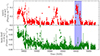 |
Fig. 1. Light curves derived from the MAXI all-sky monitor in the 2 − 20 keV range and Swift/BAT in the 15 − 50 keV range. The source transition into an extended low-flux state is clearly visible. The noteworthy resurgence of brightness in 2021, which is the primary focus of our study, is indicated in blue. |
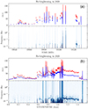 |
Fig. 2. Panel a: (top) rebrightening in 2020 in the 1 − 4 keV and 4 − 10 keV, represented by red and blue curves, respectively. (bottom) Dynamic power density spectrum (PDS) spanning the 1 − 10 keV range. Panel b: (top) the gaps between effective observations were eliminated, due to the extended timescale of the data, to enhance the clarity of the temporal evolution. The figure clearly reveals the presence of mHz QPOs ∼20 mHz, a pattern that aligns with the heartbeat state. |
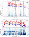 |
Fig. 3. Panel a: (top) rebrightening in 2021 in the 1 − 4 keV and 4 − 10 keV, represented by red and blue curves, respectively. (bottom) Dynamic power density spectrum spanning the 1 − 10 keV range. The five red dashed lines serve to delineate four distinct epochs characterized by different timing properties. Panel b: the gaps between effective observations were eliminated, due to the extended timescale of the data, to enhance the clarity of the temporal evolution. The figure clearly reveals the presence of LFQPOs ∼0.2 Hz and high-frequency brake noise. The five dashed lines in (a) and (b) represent the same time intervals. With the gaps removed, they more clearly distinguish the four different regions in (b). |
3.1. Timing variability
3.1.1. Power density spectrum analysis
An in-depth timing analysis of the 41 observations was performed. For each of these observations, we employed the powspec tool to generate a power density spectrum (PDS) using the screened event file within the frequency range of 1/128 − 10 Hz and in the energy band of 1 − 10 keV. The PDS was converted to a readable file for Xspec by the flx2rsp task, and we used multi-Lorentz components to fit the broadband, the peaked noises, and QPOs. For each of the four epochs mentioned earlier, we identified one observation to represent its timing properties. To show the details of their PDS fit (see Fig. 4) we chose ObsID 4647012001 for Epoch 1, ObsID 4103010241 for Epoch 2, ObsID 4647012501 for Epoch 3, and ObsID 4647012701 for Epoch 4. Each observation can be accurately fitted with three Lorentzian components, which we depict using dashed lines in blue (Lor1), purple (Lor2), and gray (Lor3). For the Lor3 component, we fixed the central frequency (F0) at 0, as it consistently represents band-limited noise that prevails below 0.1 Hz throughout the entire rebrightening period. However, it is worth noting that the other two components exhibit distinct properties across different epochs. For these two components, we maintained the flexibility to adjust all parameters during the fitting process. We used the characteristic frequency  at which it attains the maximum power in νPν and Q factor Q ≡ F0/σ to measure the narrowness of the component. The σ is the full width at half maximum (FWHM) of the Lorentz component.
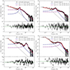 |
Fig. 4. PDSs of ObsID 4647012001 (QPO Epoch), 4103010241 (Epoch 2), 4647012501 (Epoch 3), and 4647012701 (Epoch 4) fitted with three Lorentzian components shown as blue (Lor1), purple (Lor2), and gray dashed lines. The red line indicates the sum of all components. The bottom part of each panel shows the residual of the fitting. The characteristic frequency Fc and the Q factor of the Lor1 and Lor2 components are shown in each panel. |
In ObsID 4647012001 during Epoch 1 Lor1 appears as a narrow QPO component with Fc = 0.18 ± 0.01 Hz and Q = 4.6, which is larger than 2. It becomes a wide noise component with Q < 2 in ObsID 4103010241 during Epoch 2, ObsID 4647012501 during Epoch 3, and ObsID 4647012701 during Epoch 4. The Lor2 component evolves from a band-limited noise to a peaked noise with Fc = 1.36 ± 0.02 Hz and Q = 2.0 in ObsID 4647012501 during Epoch 3 and with Fc = 1.09 ± 0.05 Hz and Q = 1.5 in ObsID 4647012701 during Epoch 4.
3.1.2. Timing properties as a function of time
In Fig. 5 we present the temporal evolution of the Lor1 and Lor2 components in the left and right panels, respectively. In the left panel the Lor1 component is a low-frequency QPO (LFQPO) with a central frequency (Fc) in the range of approximately 0.17 − 0.21 Hz. The quality factor is Q > 2 during the period between MJD 59404 and 59425 in Epoch 1. However, after MJD 59425 it makes the transition into a band-limited noise state with Q ≪ 2. In the right panel, during the QPO epoch, Lor2 appears as a band-limited noise with Fc ∼ 0.4 Hz and Q ∼ 0.5. However, at the end of the QPO epoch, the Fc increases suddenly from ∼0.4 Hz to ∼1.5 Hz, and the Q factor increases from ∼0.5 to ∼1.5. This makes Lor2 a peaked noise or even a broad QPO with Q∼ in ObsID 4647012501.
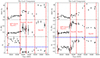 |
Fig. 5. RMS (%), Fc (Hz), and Q factor of Lor1 and Lor2 (left and right panels, respectively). The five red dashed lines serve to delineate four distinct epochs characterized by different timing properties. |
In Fig. 6, we offer a more detailed view of the QPO epoch, showing its evolution over time. We observe a gradual increase in the QPO frequency from 0.17 Hz to 0.21 Hz, with two exceptions during the dips around MJD 59412 and 59418. Additionally, the QPO’s root mean square (RMS) value shows a progressive rise over time, growing from 7% to 12%.
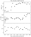 |
Fig. 6. RMS (%), Fc (Hz), and Q factor of the LFQPOs. |
3.1.3. The RMS spectrum
To study the evolution of the QPO fractional RMS with energy, we selected a joint observation of NICER and NuSTAR on July 14, 2021 (NICER: 4647012001; NuSTAR: 90701323002), within Epoch 1. Due to the effective areas of NICER and NuSTAR, we can obtain a significant broadband RMS spectrum. To account for the deadtime effect, we generated cross-power density spectra (CPDS) for the NuSTAR data, using the tool MaLTPyNT (Bachetti et al. 2015). This timing analysis package takes care of the NuSTAR dead time effect (Harrison et al. 2013; Bachetti et al. 2015). In order to check whether this method removes the deadtime effect, we compare the DPS of NICER and the CPDS of NuSTAR in 6 − 8 keV in the bottom panel of Fig. 7. The RMS spectrum of NuSTAR is shown with green points in the upper panel of Fig. 7.
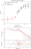 |
Fig. 7. Upper panel: evolution of the RMS with energy. The data points in red and black correspond to simultaneous observations conducted by NICER and NuSTAR on July 14, 2021 (NICER: 4647012001; NuSTAR: 90701323002). The green points show the RMS spectrum of NuSTAR from cross-power density spectra (CPDS). Bottom panel: joint fitting of the PDS in 6 − 8 keV. The black and red points show the PDS of NICER and CPDS of NuSTAR, separately. |
Regarding the white noise, instead of directly subtracting it from the PDS when generating the PDS using the powspec tool, we opted to fit it using a powerlaw function with a fixed index of 0 in order to ensure that deadtime effects did not affect the calculation of QPO RMS. For the remaining components, our fitting methodology followed the same approach outlined in Sect. 3.1.1.
For the NICER observation, light curves in the energy bands 1 − 2 keV, 2 − 3 keV, 3 − 4 keV, 4 − 5 keV, 5 − 6 keV, and 6 − 8 keV were extracted, whereas for the NuSTAR observation we chose 4 − 6 keV, 6 − 8 keV, 8 − 10 keV, 10 − 12 keV, and 12 − 18 keV. The results are shown in the upper panel of Fig. 7. From 1 to 18 keV, the QPO’s RMS overall increases from 6% to 18%. More specifically, only in the 3 − 8 keV band does the RMS clearly increase, while it stays stable at 6% in the 1 − 3 keV range, and around 18% above 8 keV.
NICER does not contain a significant QPO component above 8 keV. The PDS at 8 − 10 keV is dominated by white noise due to the low effective area at these energies, and therefore provides limited statistics. At higher energies (> 8 keV), NuSTAR has a larger effective area, allowing us to constrain the QPO signal. For energies > 18 keV the NuSTAR PDS is also dominated by white noise. This is not surprising since the count rate above 20 keV is very low for this outburst, and it is essentially dominated by the background.
3.2. The spectral analysis
3.2.1. Joint NICER and NuSTAR spectral analysis
The energy range of NICER does not allow us to obtain tight constraints on parameters of spectral components typically constrained by the hard energies. To this end, we can use the simultaneous observations by NuSTAR (ObsID: 90701323002) and NICER (ObsID: 4647012001) on July 14, 2021, in the QPO epoch. This provides us with an opportunity to validate our model through the joint fitting. For NuSTAR’s observation, limited by the background, we chose the energy range from 4 keV to 25 keV. During the fitting process, we included a 1.5% systematic error for NICER. We found that we need to add an additional 1% systematic error between 6 − 10 keV for NuSTAR, due to the limited spectral resolution for the absorption lines.
We first chose a thermally Comptonized model thcomp times the multi-blackbody components diskbb from the accretion disk, and then times the Tuebingen-Boulder ISM absorption model TBabs with abundances as in Wilms et al. (2000), and equivalent hydrogen column density nH as a free parameter. Cross-calibration between NICER and NuSTAR was carried out by the model Crabcorr(plabs) rather than a simple constant (Steiner et al. 2010; Wang et al. 2020), which could multiply each spectrum by a power law, applying corrections to both the slope via ΔΓ and normalization. In this way, the responses of different detectors were cross-calibrated to return the same normalizations and power-law slopes for the Crab. The model plabs×TBabs×thcomp×diskbb gives a reduced χ2 = 6441.94/350. The best fit exhibits substantial residuals in 2 − 5 keV, and it is not possible to derive reasonable disk parameters. It should be kept in mind that during the outburst phase there could be substantial additional absorption from neutral matters surrounding the central source; this absorption is consistently employed when modeling the spectrum during the obscured state of GRS 1915+105 (Neilsen et al. 2020; Kong et al. 2021; Liu et al. 2022). To fit this kind of absorption, we incorporated an extra component in the form of a partial covering fraction absorption model, denoted as pcfabs. The residual also leaves a prominent broad dip structure around ∼9 keV without a known origin. We then used an edge model to fit this dip. In this way, the residual contains a structure between 1 − 3 keV, leaving only narrow absorption lines. We note that the structures between 1 − 3 keV are commonly seen in NICER’s residuals, which can be attributed to calibration inaccuracy (e.g., the aluminum K edge–fluorescence at 1.56 keV, the silicon K edge from the detector window at 1.84 keV, and the gold M edge from XRC reflector gold coating at 2.2 keV1). The Fe XXV K-α line at ∼6.7 keV, the Fe XXVI Ly-α at ∼6.97 keV, the Fe XXV K-β line at ∼7.8 keV, and the Fe XXVI Ly-β line at ∼8.27 keV are very significant (see the left panel of Fig. 8). To get a more physical insight for the generation of multiple absorption lines, we used a partial covering absorption by partially ionized material model zxipcf. This model uses a grid of XSTAR photoionized absorption models for the absorption, then assumes that this only covers some fraction of the source, while the remaining (1-f) of the spectrum is seen directly (Miller et al. 2006; Reeves et al. 2008). In this situation, we chose to keep the covering fraction (represented as “f”) fixed at 1 within the zxipcf model during the fitting process due to its degeneracy with other parameters and because it primarily falls within the range of 0.8 − 1. After the fitting process, we still found a narrow dip structure at ∼8 keV, which can be fitted by another edge model. The total model is TBabs× pcfabs×zxipcf×edge×edge×thcomp×diskbb (Model 1). The results of fitting and parameters are shown in the right panel of Fig. 8 and Table 1. We observe that the presence of the two additional dip structures around 7.6 keV and 8.8 keV can be attributed to the K-edge of Co at 7.7 keV and the K-edge of Cu at 8.97 keV or potentially to the limitations of lower energy spectrum resolution within the 7–10 keV range, which may not accurately resolve the absorption lines.
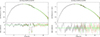 |
Fig. 8. Left panel: joint fitting result using the TBabs×pcfabs×edge×thcomp×diskbb model. Right panel: result using the TBabs×pcfabs×zxipcf×edge×edge×thcomp×diskbb model. |
Spectral parameters of joint fitting of NICER+NuSTAR.
From the fitting the equivalent hydrogen column nH from the interstellar medium (ISM), and possibly the cold matters surrounding the source, is ∼5 × 1022 cm−2, which is consistent with the typical value during the persistent outburst (Zoghbi et al. 2016; Kong et al. 2021; Liu et al. 2022). The column density of pcfabs is ∼7.5 with a cover factor 0.46. The disk temperature kTin is 1.8 keV with the normalization 30.4. The thcomp has a value Γ = 1.3, kTe = 2.8, and the cover factor is 0.05. With this model, although we can obtain acceptable residuals, we have to consider the reasonableness of the disk parameters. By considering an inclination angle of 66° and a distance of 9 kpc, we can calculate the inner radius of the accretion disk  km (Kubota et al. 1998), where Ndisk is the diskbb normalization, θ is the inclination angle, D10 is the distance in units of 10 kpc, ξ = 0.412 is the general relativity correction factor, and fcol = 1.7 is the color-correction factor with the canonical value from Shimura & Takahara (1995). Such a small value of the inner radius is far less and unreasonable for a Kerr black hole with 12 M⊙ and a = 0.98 (RISCO ∼ 1.6 GM c−2 = 28 km; Reid et al. 2014). If we assume that Rin = RISCO, we need fcol = 2.9, which is far larger than the value of a standard disk. Such a large fcol is only possible when the disk emission is relatively less dominant during the outburst of the low-mass black hole binaries (Merloni et al. 2000; Ren et al. 2022).
In this situation, the nature of the disk itself may be far beyond the geometric thin disk, or the disk may be so encased in the warm layer (Zhang et al. 2000; Gronkiewicz & Różańska 2020) that the radiation from the disk is completely diluted. This kind of warm layer is stronger in the case of the higher accretion rate and the greater magnetic field strength (Gronkiewicz & Różańska 2020). Following Zhang et al. (2000), Pszota & Cui (2007), we replace diskbb to comptt to model the disk emission with saturated Compton scattering (Titarchuk 1994). And we found the pcfabs is not needed during the spectral fitting. The total model is TBabs×zxipcf×edge×edge×thcomp×comptt (Model 2). The parameters are shown in Table 1. The T0 value for the comptt model is 0.23 keV; it is linked to kT/2.7fcol during the fitting, where fcol = 1.7, representing a standard disk (refer to Pszota & Cui 2007 for more details). At this time we found the optical depth τ is up to 57. This implies that the total emission from the accretion disk undergoes saturated Compton scattering in some low-temperature optically thick gas before the seed photons are up-scattered to higher energy levels. Because the optical depth is large, the comptt is equivalent to a 1 keV blackbody. In addition, since fcov is close to 1, the model thcomp×comptt can be simplified to the nthComp model with inp_type = 0 indicating blackbody seed photons.
Based on the analysis mentioned above, we are inclined to use the TBabs×zxipcf×edge×edge×nthComp (Model 3) for further spectral analysis. The fitting results are shown in Table 1. The overall continuum spectrum can be fitted with an nthComp model with Γ = 3.3, Tbb = 1.07, and KTe = 3.9 (see Fig. 9).
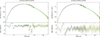 |
Fig. 9. Left panel: joint fitting result using the TBabs×edge×nthComp model. Right panel: result using the TBabs×zxipcf×edge×edge×nthComp model. |
3.2.2. Spectral evolution
We performed an analysis of the spectral evolution using all available NICER observations and by employing the TBabs×zxipcf×edge×edge×nthComp model (Model 3). The observations used for spectral evolution analysis are identical to the data utilized for timing analysis. Throughout this analysis, we maintain a fixed electron temperature of 4 keV as determined through the joint (broader band) modeling discussed in the previous section. As representative examples for spectral fitting, we chose ObsID 4647012001, which exhibits a QPO in Epoch 1, and ObsID 4647012501, which displays peaked noise (or a broad QPO with a Q factor of approximately 2) in Epoch 3. The fitting results are shown in Fig. 10 and Table 2. For ObsID 464712001, the column density Nh is ∼50 × 1022 cm−2 with a high ionization degree log ξ ∼ 4.1. The property of the absorption in ObsID 4647012001 changes into lower column density ∼13 × 1022 cm−2 and ionization degree log ξ ∼ 3.4.
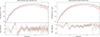 |
Fig. 10. Left panel: residuals following the inclusion of the zxipcf model of ObsID: 4647012001 (black points) and ObsID: 4647012501 (red points). Right panel: residuals excluding the zxipcf model. |
Spectral parameters of joint fitting of NICER.
During the fitting process, we found that the parameters of the two edge models remained largely unchanged for most of the observations. Therefore, we fixed Eedge1 at 7.6 keV, τedge1 at 0.1, Eedge2 at 8.8 keV and τedge2 at 0.18 for two edge models. By multiplying a cflux on nthComp, we calculated the unabsorbed flux in 1 − 10 keV of the source. The results of the evolution of the continuum spectrum parameters can be found in Fig. 11. The neutral hydrogen column density nH in TBabs remains relatively constant, predominantly within the range of 4.76 × 10²² to 5.25 × 1022 cm−2, with no significant evolution. For the ionized absorption component that we are most concerned about, we found that the column density Nh and the ionization degree log ξ exhibits higher values ∼50 × 1022 cm−2 and ∼4.1 in QPO Epoch (Epoch 1), and then decrease into lower values in Epoch 2, Epoch 3 and Epoch 4. The photon index Γ decreases from 10 to 2.5 during the whole rebrightening. The primary decline occurs during the first week after the rebrightening begins, and after that the value remains stable at 2.5. For a given kTe = 4 and photon index 2.5 < Γ < 10, we estimated the optical depth 1 < τ < 7 by the Eq. (A.1) in Zdziarski et al. (1996). The blackbody temperature, kTbb, decreases from 1.4 to 0.8. During the rebrightening, LX has many dips that correspond to spikes of Γ and kTbb at the same time. The total luminosity LX can be calculated by 4πD2FX, where D = 9 kpc.
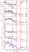 |
Fig. 11. Fitting outcomes derived from the TBabs×zxipcf×edge×edge×nthComp model (Model 3). Illustrating the evolution of neutral hydrogen absorption nH from the interstellar medium (ISM) and cold dust. It further details the wind column density Nh, the degree of wind ionization represented by log (ξ), the photon index Γ, the seed photon temperature kTbb, and the luminosity before absorption. Within the zxipcf component, the covering fraction and redshift are held constant at values of 1 and 0, respectively. From the joint fitting results, the electron temperature kTe in the nthComp model remains fixed at 4 keV. |
Here, we note that it is possible that the results on the evolution of photon index Γ and kTe are based only on phenomenology and not on real results. Due to the limitations of the NICER energy band, we can only approximate the value of kTe based on the only NuSTAR observation. The evolution of Γ obtained by fixing kTe may be incorrect since kTe itself is likely to evolve during the rebrightening. Since the parameters of the ionized absorption model zxipcf do not have degeneracy with Γ and kTe, we consider their evolution to be reliable.
4. Discussions
This work presents a detailed timing-spectral analysis of the NICER observations relative to the X-ray rebrightening of GRS 1915+105 in 2021. Compared to the hard state before entering the low-flux state (t < MJD 58600), although the flux below 20 keV of the whole rebrightening is similar to the hard state, the flux above 20 keV has significantly decreased (see Fig. 1). The key finding of our analysis is that the spectral and timing properties of the source during the rebrightening phase exhibit significant differences compared to those typical of the soft and hard states of black hole binaries.
The emission is dominated by the Comptonization of seed photons within the optically thick low-temperature plasma and displays ionized absorption lines. The numerous absorption lines in the spectrum indicate that photons have interacted with an ionized absorbing medium, whose properties undergo significant changes throughout the rebrightening phase. More specifically the plasma evolves from higher column density Nh ∼ 50 × 1022 cm−2 and ionization degree log ξ ∼ 4 to the lower column density Nh ∼ 10 × 1022 cm−2 and ionization degree log ξ ∼ 3.5. What is even more intriguing is that during this soft X-ray rebrightening QPOs are observed up to an energy of 18 keV (see the upper panel of Fig. 7). The QPOs exhibit a relatively weak evolution in terms of frequency spanning the range of 0.17 − 0.21 Hz. By comparing Figs. 5 and 11, it becomes evident that the QPOs only manifest within the initial 20 days following the onset of the rebrightening. This coincides with the phase in which the absorbing medium exhibits high column density and ionization degree. After the PDS evolves from a QPO signal superimposed on a low-frequency broadband-limited noise into a high-frequency peaked noise superimposed on a low-frequency broadband noise (see Fig. 4), the column density and ionization degree decrease. Figure 6 clearly shows the QPO’s properties. In particular, although the frequency of QPO increases with time from 0.17 Hz to 0.21 Hz, there are three sudden decreases, which correspond precisely to the sudden increase in the Γ and kTbb parameters and to the decrease in flux at MJD 58411, MJD 58417, and MJD 58423 (see Fig. 11). As mentioned earlier, when using the nthComp model we assume a constant electron temperature obtained from the only NICER and NuSTAR joint observation during the rebrightening episode. In addition, the model we use differs significantly from typical models employed in modeling the X-ray emission of black hole binary systems. We can get a good fitting by using a canonical model like tbabs×pcfabs×thcomp×diskbb, but as we discussed above, this model cannot give a reasonable inner radius of the accretion disk. The diskbb should be abandoned in the fitting; this means that the emission from the accretion disk might be totally covered by the optically thick and low-temperature electrons, which can be modeled by a saturated Compton scattering model comptt. In summary, our findings regarding the soft X-ray rebrightening in 2021 indicate that the radiation is predominantly dominated by Compton-thick low-temperature electrons accompanied by a QPO signal below 18 keV. Furthermore, the appearance and disappearance of these QPOs are correlated with the characteristics of the absorbing material surrounding the source. Specifically, QPOs only manifest when the absorbing medium shows high column densities and a high ionization degree. In our following discussion, the purpose is to discuss the origin of such unique low-frequency QPOs based on the properties of QPOs and the results of the spectral fitting.
4.1. The specificity of state and QPO property
As we know, both in typical transient BHs or GRS 1915+105, a spectrum can be classified as soft state (SS), hard state (HS), or intermediate state (IMS; Belloni 2010). The LFQPOs are usually found in the hard state or intermediate state (Ingram & Motta 2019).
The peak unabsorbed and/or intrinsic luminosity in 1 − 10 keV of this rebrightening is ∼4 × 1037 erg s−1 which is 0.03 LEdd (assuming a BH mass of 12 M⊙; Reid et al. 2014). This flux level is comparable to that in the decay at MJD 58220 − 58330 and to the peak flux of the soft X-ray rebrightening in 2020 (MJD 59100; Koljonen & Hovatta 2021; Motta et al. 2021). However, a significant difference is that the decay state is more consistent with a hard state. Compared with the soft state around MJD 58000 (see Motta et al. 2021), the flux of the soft X-ray rebrightening in 2021 is lower, and the duration of the soft emission is shorter.
Meanwhile, the type-C QPOs around 0.17 Hz emerge during the initial phase of the soft X-ray rebrightening in 2021. Such time-varying signals are typically more prevalent in the hard state than in the soft state. This rebrightening phenomenon deviates once again from the characteristics of a typical soft state in this regard. Zhang et al. (2020) presented a systematic analysis of the type-C quasi-periodic oscillations (QPOs) in GRS 1915+105 using RXTE data. The statistical analysis reveals that the frequency distribution of type-C QPOs falls within the range of 0.4–6.4 Hz, with the upper limit extending to 40 keV in terms of high-energy observations. The case is different in our work. We observed that the QPOs in the initial phase of the rebrightening fall within a significantly lower frequency range of ∼0.17 − 0.21 Hz. As shown in the upper panel of Fig. 7, although the increasing trend of the QPO RMS spectrum is similar to that of the QPO in Zhang et al. (2020), the maximum energy that QPOs and the frequency that QPOs can reach are entirely different. Such a trend of increasing RMS with multiple scattering events indicates that seed photons undergoing more scatterings exhibit higher RMS values. The QPO signal does not originate from the incident photons; instead, it arises from the scattering plasma, that is from the electrons. This conclusion aligns with the origin of QPOs in typical black hole systems being consistent with the corona. Compared to the corona temperatures reaching 50 − 100 keV during typical outbursts, an electron temperature of 4 keV makes it challenging for seed photons to scatter to energies above 20 keV. Consequently, this prevents us from observing QPO signals at higher energy levels.
4.2. The properties of the absorber
Absorption lines with blueshift speeds from 100 km s−1 to 0.1 c provide evidence of the presence of disk winds driven by thermal pressure (Tombesi et al. 2010; Done et al. 2018), radiation pressure (e.g., Higginbottom & Proga 2015), or magnetic pressure or centrifugal forces (Fukumura et al. 2010, 2017). Based on the fitting results, we observe that blueshift and redshift values are nearly zero for nearly all observations, which is why we held them constant at 0. This suggests that the absorber exhibited slow movement along the line of sight. In our case it may be more in line with a failed wind during the obscured state of GRS 1915+105 with low flux level (Miller et al. 2020). From the parameters of the zxipcf model we can estimate the upper limit of the launch radius Rlaunch according to the equation (Tarter et al. 1969)
 (1)
(1)
where L is the luminosity. Here we take the results at the rebrightening peak, L ∼ 3.83 × 1037 erg s−1 (0.025 Ledd), Nh ∼ 34 − 98 × 1022 cm−2, and log ξ ∼ 4.1, and obtain RLaunch ≤ 3 − 9 × 10⁴ km. Dubus et al. (2019) considered the contribution from radiation pressure at luminosity close to Eddington (Proga & Kallman 2002; Done et al. 2018). Accordingly, the equation for TIC and RIC is shown as
 (2)
(2)
 (3)
(3)
where l = L/Ledd. The Compton temperature TIC and Compton radius RIC can be estimated as 0.69 × 10⁷ K and 1.1 × 10⁷ km, respectively. Since RLaunch is 0.003 RIC, which is far less than 0.2 RIC, the absorber is not likely thermal driven (Woods et al. 1996). Therefore, we assume the absorber is a Compton-thick magnetically driven failed disk wind. Similarly, we can also estimate RLaunch ≤ 4.5 − 9 × 10⁵ km, TIC ∼ 5.58 × 10⁷ K, and RIC ∼ 2.1 × 10⁶ km at lower Nh ∼ 7 − 14 × 1022 erg s−1, log ξ ∼ 3.5 and luminosity L ∼ 2 × 1037 erg s−1 (0.01 LEdd). The value of RLaunch ∼ 0.21 − 0.43 RIC is near the threshold 0.2 RIC, which means that the thermally driven case cannot be excluded here.
The above calculation makes it easy to find that the driving mechanism and position of the failed wind vary significantly at different luminosities or accretion rates. In the QPO epoch, the luminosity is high, and the wind is generated closer to the black hole (RLaunch ∼ 0.003 RIC). In this case it may be driven by the magnetic pressure on the disk and maintained in equilibrium with gravity (although the redshift or blueshift is very low, we cannot exclude that the disk wind has a significant speed in the direction perpendicular to the disk because GRS 1915+105 is highly inclined binary. At lower luminosity, when there is no QPO signal, the winds are generated farther away from the black hole (RLaunch ∼ 0.21 − 0.43 RIC) when they might be thermally driven.
4.3. The origin of QPOs
We found a long-duration LFQPO with ∼0.17 − 0.21 Hz appearing during the soft X-ray rebrightening. Compared with the properties of typical type-C QPOs, the frequency is lower than the lowest value in Zhang et al. (2020). The maximum energy of the observed QPO is 18 keV, which is much lower than the oscillation at 100 keV that a type-C QPO can achieve (Huang et al. 2018; Ma et al. 2021). Compared to a type-C QPO, this QPO is found to be produced in a Compton-thick low-temperature gas. Determining the composition of the accretion disk from the energy spectrum is challenging due to the potential complete shielding by the surrounding Compton-thick gas. This situation makes it impossible to collect information about the radiation within the Compton-thick gas, as any seed photon from the accretion disk scatters within this medium, ultimately generating blackbody photons and resulting in the loss of its original information. Therefore, the gas’s state and geometric distribution differ significantly from the typical corona or jet. More interestingly, the appearance of QPOs corresponds to the formation of a magnetically driven failed wind that might be the source of this Compton-thick gas (Miller et al. 2020). Considering that this gas originates much farther from the black hole, explaining the generation of LFQPO through a geometric progression caused by the Lense–Thirring effect might not be true. Given the previously mentioned direct correlation between the QPO and the Compton-thick magnetically driven failed wind, it is plausible to speculate that the mechanism for generation might arise from perturbations in the magnetic field being transmitted into the failed disk wind. This process bears a resemblance to the one outlined in the Accretion Ejection Instability (AEI) model (Tagger & Pellat 1999), which elucidates the instability of spiral waves in the density and scale height of a thin disk interlaced with a robust vertical (poloidal) magnetic field. Moreover, spiral waves not only introduce additional instability but also shape the Rossby vortex at the corotation radius. Subsequently, this vortex induces a twisting of the field lines that traverse this region, leading to the initiation of a vertical Alfven wave. This wave has the ability to transfer both energy and angular momentum from the disk to the corona, thereby playing a crucial role in initiating the formation of a wind and/or jet (Ingram & Motta 2019). However, once the mechanism shifts toward being thermally driven, the decoupling of the wind and magnetic fields formed in the outer regions leads to the dissipation of perturbations. Consequently, the QPO also ceases to exist.
5. Conclusions
We observed magnetically driven and thermal-driven transitions during a notable soft X-ray rebrightening in 2021. Remarkably, these transitions gave rise to a low-speed failed wind that formed a dense Compton-thick structure. During the magnetically driven period, it exhibited elevated ionization and column density levels. We propose that perturbation within the magnetic field can transmit into the Compton-thick gas and trigger the emergence of LFQPO signals. This shares many similarities with the AEI model. This reveals a magnetic-related perturbation mechanism hitherto unexplored in the generation of LFQPOs. We eagerly anticipate additional theoretical investigations and observational evidence to substantiate this conjecture.
Acknowledgments
This research has made use of data obtained from the High Energy Astrophysics Science Archive Research Center (HEASARC), provided by NASA’s Goddard Space Flight Center. This work is grateful for the financial support provided by the Sino-German (CSC-DAAD) Postdoc Scholarship Program, 2022 (57607866). This work is supported by the National Natural Science Foundation of China under grant No. 12173103. This work is also supported by the National Key R&D Program of China (2021YFA0718500).
References
- Arnaud, K. A. 1996, in Astronomical Data Analysis Software and Systems V, eds. G. H. Jacoby, & J. Barnes, ASP Conf. Ser., 101, 17 [NASA ADS] [Google Scholar]
- Athulya, M. P., Radhika, D., Agrawal, V. K., et al. 2022, MNRAS, 510, 3019 [NASA ADS] [CrossRef] [Google Scholar]
- Bachetti, M., Harrison, F. A., Cook, R., et al. 2015, ApJ, 800, 109 [NASA ADS] [CrossRef] [Google Scholar]
- Balakrishnan, M., Miller, J. M., Reynolds, M. T., et al. 2021, ApJ, 909, 41 [NASA ADS] [CrossRef] [Google Scholar]
- Belloni, T. M. 2010, in Lect. Notes Phys., ed. T. Belloni (Berlin Springer Verlag), 794, 53 [NASA ADS] [CrossRef] [Google Scholar]
- Belloni, T., Klein-Wolt, M., Méndez, M., van der Klis, M., & van Paradijs, J. 2000, A&A, 355, 271 [Google Scholar]
- Castro-Tirado, A. J., Brandt, S., & Lund, N. 1992, IAU Circ., 5590, 2 [NASA ADS] [Google Scholar]
- Done, C., Tomaru, R., & Takahashi, T. 2018, MNRAS, 473, 838 [NASA ADS] [CrossRef] [Google Scholar]
- Dubus, G., Done, C., Tetarenko, B. E., & Hameury, J.-M. 2019, A&A, 632, A40 [NASA ADS] [CrossRef] [EDP Sciences] [Google Scholar]
- Egron, E., Rodriguez, J., Trushkin, S. A., et al. 2023, ATel, 16008, 1 [NASA ADS] [Google Scholar]
- Fukumura, K., Kazanas, D., Contopoulos, I., & Behar, E. 2010, ApJ, 715, 636 [NASA ADS] [CrossRef] [Google Scholar]
- Fukumura, K., Kazanas, D., Shrader, C., et al. 2017, Nat. Astron., 1, 0062 [NASA ADS] [CrossRef] [Google Scholar]
- Gendreau, K. C., Arzoumanian, Z., Adkins, P. W., et al. 2016, in Space Telescopes and Instrumentation 2016: Ultraviolet to Gamma Ray, eds. J. W. A. den Herder, T. Takahashi, & M. Bautz, SPIE Conf. Ser., 9905, 99051H [NASA ADS] [CrossRef] [Google Scholar]
- Greiner, J., Cuby, J. G., McCaughrean, M. J., Castro-Tirado, A. J., & Mennickent, R. E. 2001, A&A, 373, L37 [NASA ADS] [CrossRef] [EDP Sciences] [Google Scholar]
- Gronkiewicz, D., & Różańska, A. 2020, A&A, 633, A35 [NASA ADS] [CrossRef] [EDP Sciences] [Google Scholar]
- Hannikainen, D. C., Rodriguez, J., Vilhu, O., et al. 2005, A&A, 435, 995 [NASA ADS] [CrossRef] [EDP Sciences] [Google Scholar]
- Harrison, F. A., Craig, W. W., Christensen, F. E., et al. 2013, ApJ, 770, 103 [Google Scholar]
- Higginbottom, N., & Proga, D. 2015, ApJ, 807, 107 [Google Scholar]
- Homan, J., Neilsen, J., Allen, J. L., et al. 2016, ApJ, 830, L5 [Google Scholar]
- Homan, J., Neilsen, J., Gendreau, K., et al. 2019, ATel, 13308, 1 [NASA ADS] [Google Scholar]
- Huang, Y., Qu, J. L., Zhang, S. N., et al. 2018, ApJ, 866, 122 [NASA ADS] [CrossRef] [Google Scholar]
- Huppenkothen, D., Bachetti, M., Stevens, A., et al. 2019a, J. Open Source Softw., 4, 1393 [NASA ADS] [CrossRef] [Google Scholar]
- Huppenkothen, D., Bachetti, M., Stevens, A. L., et al. 2019b, ApJ, 881, 39 [Google Scholar]
- Ingram, A. R., & Motta, S. E. 2019, New Astron. Rev., 85, 101524 [Google Scholar]
- Kaastra, J. S., & Bleeker, J. A. M. 2016, A&A, 587, A151 [NASA ADS] [CrossRef] [EDP Sciences] [Google Scholar]
- Klein-Wolt, M., Fender, R. P., Pooley, G. G., et al. 2002, MNRAS, 331, 745 [Google Scholar]
- Koljonen, K. I. I., & Hovatta, T. 2021, A&A, 647, A173 [NASA ADS] [CrossRef] [EDP Sciences] [Google Scholar]
- Koljonen, K. I. I., & Tomsick, J. A. 2020, A&A, 639, A13 [EDP Sciences] [Google Scholar]
- Koljonen, K., Vera, R., Lahteenmaki, A., & Tornikoski, M. 2019, ATel, 12839, 1 [Google Scholar]
- Kong, L. D., Zhang, S., Chen, Y. P., et al. 2021, ApJ, 906, L2 [NASA ADS] [CrossRef] [Google Scholar]
- Kubota, A., Tanaka, Y., Makishima, K., et al. 1998, PASJ, 50, 667 [NASA ADS] [CrossRef] [Google Scholar]
- Leahy, D. A., Darbro, W., Elsner, R. F., et al. 1983, ApJ, 266, 160 [NASA ADS] [CrossRef] [Google Scholar]
- Liu, H., Fu, Y., Bambi, C., et al. 2022, ApJ, 933, 122 [NASA ADS] [CrossRef] [Google Scholar]
- Ma, X., Tao, L., Zhang, S.-N., et al. 2021, Nat. Astron., 5, 94 [NASA ADS] [CrossRef] [Google Scholar]
- Merloni, A., Fabian, A. C., & Ross, R. R. 2000, MNRAS, 313, 193 [NASA ADS] [CrossRef] [Google Scholar]
- Miller, L., Turner, T. J., Reeves, J. N., et al. 2006, A&A, 453, L13 [NASA ADS] [CrossRef] [EDP Sciences] [Google Scholar]
- Miller, J. M., Zoghbi, A., Raymond, J., et al. 2020, ApJ, 904, 30 [Google Scholar]
- Motta, S. E., Kajava, J. J. E., Giustini, M., et al. 2021, MNRAS, 503, 152 [Google Scholar]
- Murata, K. L., Kawai, N., Yamagishi, M., et al. 2019, ATel, 12769, 1 [NASA ADS] [Google Scholar]
- Neilsen, J., & Lee, J. C. 2009, Nature, 458, 481 [NASA ADS] [CrossRef] [Google Scholar]
- Neilsen, J., Remillard, R. A., & Lee, J. C. 2011, ApJ, 737, 69 [Google Scholar]
- Neilsen, J., Homan, J., Steiner, J. F., et al. 2020, ApJ, 902, 152 [Google Scholar]
- Neilsen, J., Altamirano, D., Homan, J., et al. 2021, ATel, 14792, 1 [NASA ADS] [Google Scholar]
- Ponti, G., Fender, R. P., Begelman, M. C., et al. 2012, MNRAS, 422, L11 [NASA ADS] [CrossRef] [Google Scholar]
- Proga, D., & Kallman, T. R. 2002, ApJ, 565, 455 [NASA ADS] [CrossRef] [Google Scholar]
- Pszota, G., & Cui, W. 2007, ApJ, 663, 1201 [CrossRef] [Google Scholar]
- Ratheesh, A., Tombesi, F., Fukumura, K., et al. 2021, A&A, 646, A154 [NASA ADS] [CrossRef] [EDP Sciences] [Google Scholar]
- Ravishankar, B. T., Tilak, K., Athulya, M. P., et al. 2021, ATel, 14811, 1 [NASA ADS] [Google Scholar]
- Reeves, J., Done, C., Pounds, K., et al. 2008, MNRAS, 385, L108 [Google Scholar]
- Reid, M. J., McClintock, J. E., Steiner, J. F., et al. 2014, ApJ, 796, 2 [Google Scholar]
- Ren, X. Q., Wang, Y., Zhang, S. N., et al. 2022, ApJ, 932, 66 [NASA ADS] [CrossRef] [Google Scholar]
- Sanchez-Sierras, J., Munoz-Darias, T., Motta, S., Fender, R., & Bahramian, A. 2023, ATel, 16039, 1 [Google Scholar]
- Shimura, T., & Takahara, F. 1995, ApJ, 445, 780 [Google Scholar]
- Steiner, J. F., McClintock, J. E., Remillard, R. A., et al. 2010, ApJ, 718, L117 [Google Scholar]
- Stella, L., & Angelini, L. 1992, in Astronomical Data Analysis Software and Systems I, eds. D. M. Worrall, C. Biemesderfer, & J. Barnes, ASP Conf. Ser., 25, 103 [Google Scholar]
- Tagger, M., & Pellat, R. 1999, A&A, 349, 1003 [NASA ADS] [Google Scholar]
- Tarter, C. B., Tucker, W. H., & Salpeter, E. E. 1969, ApJ, 156, 943 [Google Scholar]
- Titarchuk, L. 1994, ApJ, 434, 570 [NASA ADS] [CrossRef] [Google Scholar]
- Tombesi, F., Cappi, M., Reeves, J. N., et al. 2010, A&A, 521, A57 [NASA ADS] [CrossRef] [EDP Sciences] [Google Scholar]
- Trushkin, S. A., Nizhelskij, N. A., Tsybulev, P. G., Bursov, N. N., & Shevchenko, A. V. 2019a, ATel, 12855, 1 [Google Scholar]
- Trushkin, S. A., Nizhelskij, N. A., Tsybulev, P. G., Bursov, N. N., & Shevchenko, A. V. 2019b, ATel, 13304, 1 [NASA ADS] [Google Scholar]
- Trushkin, S. A., Nizhelskij, N. A., Tsybulev, P. G., Bursov, N. N., & Shevchenko, A. V. 2020, ATel, 13442, 1 [Google Scholar]
- Trushkin, S. A., Nizhelskij, N. A., Tsybulev, P. G., & Shevchenko, A. V. 2023, ATel, 15964, 1 [NASA ADS] [Google Scholar]
- Vishal, J., Banerjee, & Dipankar, K. P. 2019, ATel, 12806, 1 [NASA ADS] [Google Scholar]
- Wang, J., Kara, E., Steiner, J. F., et al. 2020, ApJ, 899, 44 [NASA ADS] [CrossRef] [Google Scholar]
- Wilms, J., Allen, A., & McCray, R. 2000, ApJ, 542, 914 [Google Scholar]
- Woods, D. T., Klein, R. I., Castor, J. I., McKee, C. F., & Bell, J. B. 1996, ApJ, 461, 767 [NASA ADS] [CrossRef] [Google Scholar]
- Zdziarski, A. A., Johnson, W. N., & Magdziarz, P. 1996, MNRAS, 283, 193 [NASA ADS] [CrossRef] [Google Scholar]
- Zhang, S. N., Cui, W., Chen, W., et al. 2000, Science, 287, 1239 [Google Scholar]
- Zhang, L., Méndez, M., Altamirano, D., et al. 2020, MNRAS, 494, 1375 [Google Scholar]
- Zoghbi, A., Miller, J. M., King, A. L., et al. 2016, ApJ, 833, 165 [NASA ADS] [CrossRef] [Google Scholar]
All Tables
All Figures
|
Fig. 1. Light curves derived from the MAXI all-sky monitor in the 2 − 20 keV range and Swift/BAT in the 15 − 50 keV range. The source transition into an extended low-flux state is clearly visible. The noteworthy resurgence of brightness in 2021, which is the primary focus of our study, is indicated in blue. |
| In the text | |
|
Fig. 2. Panel a: (top) rebrightening in 2020 in the 1 − 4 keV and 4 − 10 keV, represented by red and blue curves, respectively. (bottom) Dynamic power density spectrum (PDS) spanning the 1 − 10 keV range. Panel b: (top) the gaps between effective observations were eliminated, due to the extended timescale of the data, to enhance the clarity of the temporal evolution. The figure clearly reveals the presence of mHz QPOs ∼20 mHz, a pattern that aligns with the heartbeat state. |
| In the text | |
|
Fig. 3. Panel a: (top) rebrightening in 2021 in the 1 − 4 keV and 4 − 10 keV, represented by red and blue curves, respectively. (bottom) Dynamic power density spectrum spanning the 1 − 10 keV range. The five red dashed lines serve to delineate four distinct epochs characterized by different timing properties. Panel b: the gaps between effective observations were eliminated, due to the extended timescale of the data, to enhance the clarity of the temporal evolution. The figure clearly reveals the presence of LFQPOs ∼0.2 Hz and high-frequency brake noise. The five dashed lines in (a) and (b) represent the same time intervals. With the gaps removed, they more clearly distinguish the four different regions in (b). |
| In the text | |
|
Fig. 4. PDSs of ObsID 4647012001 (QPO Epoch), 4103010241 (Epoch 2), 4647012501 (Epoch 3), and 4647012701 (Epoch 4) fitted with three Lorentzian components shown as blue (Lor1), purple (Lor2), and gray dashed lines. The red line indicates the sum of all components. The bottom part of each panel shows the residual of the fitting. The characteristic frequency Fc and the Q factor of the Lor1 and Lor2 components are shown in each panel. |
| In the text | |
|
Fig. 5. RMS (%), Fc (Hz), and Q factor of Lor1 and Lor2 (left and right panels, respectively). The five red dashed lines serve to delineate four distinct epochs characterized by different timing properties. |
| In the text | |
|
Fig. 6. RMS (%), Fc (Hz), and Q factor of the LFQPOs. |
| In the text | |
|
Fig. 7. Upper panel: evolution of the RMS with energy. The data points in red and black correspond to simultaneous observations conducted by NICER and NuSTAR on July 14, 2021 (NICER: 4647012001; NuSTAR: 90701323002). The green points show the RMS spectrum of NuSTAR from cross-power density spectra (CPDS). Bottom panel: joint fitting of the PDS in 6 − 8 keV. The black and red points show the PDS of NICER and CPDS of NuSTAR, separately. |
| In the text | |
|
Fig. 8. Left panel: joint fitting result using the TBabs×pcfabs×edge×thcomp×diskbb model. Right panel: result using the TBabs×pcfabs×zxipcf×edge×edge×thcomp×diskbb model. |
| In the text | |
|
Fig. 9. Left panel: joint fitting result using the TBabs×edge×nthComp model. Right panel: result using the TBabs×zxipcf×edge×edge×nthComp model. |
| In the text | |
|
Fig. 10. Left panel: residuals following the inclusion of the zxipcf model of ObsID: 4647012001 (black points) and ObsID: 4647012501 (red points). Right panel: residuals excluding the zxipcf model. |
| In the text | |
|
Fig. 11. Fitting outcomes derived from the TBabs×zxipcf×edge×edge×nthComp model (Model 3). Illustrating the evolution of neutral hydrogen absorption nH from the interstellar medium (ISM) and cold dust. It further details the wind column density Nh, the degree of wind ionization represented by log (ξ), the photon index Γ, the seed photon temperature kTbb, and the luminosity before absorption. Within the zxipcf component, the covering fraction and redshift are held constant at values of 1 and 0, respectively. From the joint fitting results, the electron temperature kTe in the nthComp model remains fixed at 4 keV. |
| In the text | |
Current usage metrics show cumulative count of Article Views (full-text article views including HTML views, PDF and ePub downloads, according to the available data) and Abstracts Views on Vision4Press platform.
Data correspond to usage on the plateform after 2015. The current usage metrics is available 48-96 hours after online publication and is updated daily on week days.
Initial download of the metrics may take a while.