| Issue |
A&A
Volume 696, April 2025
|
|
|---|---|---|
| Article Number | A57 | |
| Number of page(s) | 19 | |
| Section | Extragalactic astronomy | |
| DOI | https://doi.org/10.1051/0004-6361/202451723 | |
| Published online | 04 April 2025 | |
MIRI Deep Imaging Survey (MIDIS) of the Hubble Ultra Deep Field
Survey description and early results for the galaxy population detected at 5.6 μm⋆
1
Department of Astronomy, Oskar Klein Centre, Stockholm University, AlbaNova University Center, 10691 Stockholm, Sweden
2
Centro de Astrobiología (CAB), CSIC-INTA, Ctra. de Ajalvir km 4, Torrej’on de Ardoz, 28850 Madrid, Spain
3
DTU Space, Technical University of Denmark, Elektrovej 327, 2800 Kgs. Lyngby, Denmark
4
Kapteyn Astronomical Institute, University of Groningen, PO Box 800 9700 AV Groningen, The Netherlands
5
Max-Planck-Institut für Astronomie, Königstuhl 17, 69117 Heidelberg, Germany
6
Cosmic Dawn Centre (DAWN), Copenhagen, Denmark
7
UK Astronomy Technology Centre, Royal Observatory Edinburgh, Blackford Hill, Edinburgh EH9 3HJ, UK
8
Department of Physics and Astronomy, University College London, Gower Place, London WC1E 6BT, UK
9
Institute for Theoretical Physics, Heidelberg University, Heidelberg, Germany
10
I. Physikalisches Institut der Universität zu Köln, Zülpicher Str. 77, 50937 Köln, Germany
11
European Space Agency, Space Telescope Science Institute, Baltimore, MD, USA
12
DARK, Niels Bohr Institute, University of Copenhagen, Jagtvej 155A, 2200 Copenhagen, Denmark
13
Aix Marseille Université, CNRS, LAM (Laboratoire d’Astrophysique de Marseille) UMR 7326, 13388 Marseille, France
14
AURA for the European Space Agency (ESA), Space Telescope Science Institute, 3700 San Martin Drive, Baltimore, MD, USA
15
Department of Astronomy, University of Geneva, Chemin Pegasi 51, 1290 Versoix, Switzerland
16
European Space Agency (ESA), European Space Astronomy Centre (ESAC), Camino Bajo del Castillo s/n, 28692 Villaneuva de la Canada, Madrid, Spain
17
School of Physics & Astronomy, Space Park Leicester, University of Leicester, 92 Corporation Road, Leicester LE4 5SP, UK
18
Dublin Institute for Advanced Studies, Astronomy & Astrophysics Section, 31 Fitzwilliam Place, Dublin 2, Ireland
19
Centre for Extragalactic Astronomy, Durham University, South Road Durham DH1 3LE, UK
20
Leiden Observatory, Leiden University, PO Box 9513 2300 RA Leiden, The Netherlands
21
University of Vienna, Department of Astrophysics, Türkenschanzstrasse 17, 1180 Vienna, Austria
22
Institute of Particle Physics and Astrophysics, ETH Zürich, Wolfgang-Pauli-Str 27, 8093 Zurich, Switzerland
23
AIM, CEA, CNRS, Université Paris-Saclay, Université Paris Diderot, Sorbonne Paris Cité, 91191 Gif-sur-Yvette, France
24
Institute of Astronomy, KU Leuven, Celestijnenlaan 200D bus 2401, 3001 Leuven, Belgium
25
Centro de Astrobiología (CAB), CSIC-INTA, Camino Bajo del Castillo s/n, E-28692 Villanueva de la Cañada, Madrid, Spain
26
Telespazio UK for the European Space Agency (ESA), ESAC, Camino Bajo del Castillo s/n, 28692 Villanueva de la Cañada, Spain
27
Steward Observatory, University of Arizona, 933 North Cherry Avenue, Tucson, AZ 85721, USA
28
INAF – Osservatorio Astronomico di Padova, Vicolo dell’Osservatorio 5, Padova I-35122, Italy
29
Institute of Science and Technology Austria (ISTA), Am Campus 1, 3400 Klosterneuburg, Austria
30
Max-Planck-Institut für Radioastronomie (MPIfR), Auf dem Hügel 69, D-53121 Bonn, Germany
⋆⋆ Corresponding author; This email address is being protected from spambots. You need JavaScript enabled to view it.
Received:
30
July
2024
Accepted:
13
February
2025
Abstract
Context. The recently launched James Webb Space Telescope (JWST) is opening new observing windows on the distant Universe. Among JWST’s instruments, the Mid Infrared Instrument (MIRI) offers the unique capability of imaging observations at wavelengths of λ > 5 μm. This enables unique access to the rest frame near-infrared (NIR, λ ≥ 1 μm) emission from galaxies at redshifts of z > 4 and the visual (λ ≳ 5000 Å) rest frame for z > 9. We report here on the guaranteed time observations (GTO), from the MIRI European Consortium, of the Hubble Ultra Deep Field (HUDF), forming the MIRI Deep Imaging Survey (MIDIS), consisting of an on source integration time of ∼41 hours in the MIRI/F560W (5.6 μm) filter. The F560W filter was selected since it would produce the deepest data in terms of AB magnitudes in a given time. To our knowledge, this constitutes the longest single filter exposure obtained with JWST of an extragalactic field as of yet.
Aims. The HUDF is one of the most observed extragalactic fields, with extensive multi-wavelength coverage, where (before JWST) galaxies up to z ∼ 7 have been confirmed, and at z > 10 suggested, from HST photometry. We aim to characterise the galaxy population in HUDF at 5.6 μm, enabling studies such as: the rest frame NIR morphologies for galaxies at z ≲ 4.6, probing mature stellar populations and emission lines in z > 6 sources, intrinsically red and dusty galaxies, and active galactic nuclei (AGNs) and their host galaxies at intermediate redshifts.
Methods. We reduced the MIRI data using the official JWST pipeline, augmented by in-house custom scripts. We measured the noise characteristics of the resulting image. Galaxy photometry was obtained, and photometric redshifts were estimated for sources with available multi-wavelength photometry (and compared to spectroscopic redshifts when available).
Results. Over the deepest part of our image, the 5σ point source limit is 28.65 mag AB (12.6 nJy), ∼0.35 mag better than predicted by the JWST exposure time calculator. We find ∼2500 sources, the overwhelming majority of which are distant galaxies, but we note that spurious sources likely remain at faint magnitudes due to imperfect cosmic ray rejection in the JWST pipeline. More than 500 galaxies with available spectroscopic redshifts, up to z ≈ 11, have been identified, the majority of which are at z < 6. More than 1000 galaxies have reliable photometric redshift estimates, of which ∼25 are at 6 < z < 12. The point spread function in the F560W filter has a full width at half maximum (FWHM) of ≈0.2″ (corresponding to 1.4 kpc at z = 4), allowing the NIR rest frame morphologies and stellar mass distributions to be resolved for z < 4.5. Moreover, > 100 objects with very red NIRCam vs MIRI (3.6–5.6 μm > 1 mag) colours have been found, suggestive of dusty or old stellar populations at high redshifts.
Conclusions. We conclude that MIDIS surpasses preflight expectations and that deep MIRI imaging has great potential to characterise the galaxy population from cosmic noon to dawn.
Key words: galaxies: evolution / galaxies: formation / galaxies: high-redshift / infrared: galaxies
Based on results from the MIRI European Consortium Guaranteed Time Observations, programme 1283.
Deceased.
© The Authors 2025
 Open Access article, published by EDP Sciences, under the terms of the Creative Commons Attribution License (https://creativecommons.org/licenses/by/4.0), which permits unrestricted use, distribution, and reproduction in any medium, provided the original work is properly cited.
This article is published in open access under the Subscribe to Open model. This email address is being protected from spambots. You need JavaScript enabled to view it. to support open access publication.
1. Introduction
The late 1990s marked a revolution in the study of the high-redshift Universe. This was made possible through new facilities such as the Hubble Space Telescope (HST), and 8–10 m class ground-based telescopes such as the Keck and its successors, notably the ESO/VLT. While before, redshifts of z > 1 were mostly the domain of quasi-stellar objects (QSOs) and radio galaxies (see Giavalisco 2002, for a review), breakthroughs such as the Lyman break technique (Steidel & Hamilton 1992; Steidel et al. 1996a, implying dropouts in the bluer filters due to a redshifted Lyman break), more sensitive narrow-band surveys for Lyman α (Lyα) emitters (Hu et al. 1998), and not least the advent of the Hubble Deep Field (HDF, Williams et al. 1996) dramatically changed the picture (Steidel et al. 1996b; Williams 2018). The HDF was an ambitious undertaking by imaging an apparently blank and almost starless field at high Galactic latitude with HST in several filters with exposure times amounting to 30–40 hours per filter in U, B, V, and I. The HDF was found to be anything but blank, containing thousands of distant galaxies, and triggered a wealth of high-z studies (Williams 2018). Spectroscopic campaigns confirmed many galaxies in the HDF to be at high redshifts, and dropout and photometric redshift techniques could show with high probability that many sources too faint for ground-based spectroscopy are likely to reside at very high redshifts (Williams 2018). The HDF was followed over the years by several other deep field campaigns from the ground, and notably with the HST, for instance HDF-south (Williams et al. 2000), GOODS (Great Observatories Origins Deep Survey Giavalisco et al. 2004), and the Hubble Ultra Deep Field (HUDF, Beckwidth et al. 2016), which is contained within the GOODS south (GOODS-S) field. Such deep field studies aim to explore when galaxies formed and how they have evolved over cosmic time.
At redshifts of z ≳ 4, the absorption by neutral hydrogen in the intergalactic medium (IGM) efficiently suppresses any emission bluewards of Lyα, meaning that the ‘dropouts’ would mainly trace the Lyα break (1216Å) rather than the Lyman discontinuity (912 Å, Madau 1995; Inoue et al. 2014). With optical-only observations, this originally limited dropout studies with HST to z < 6. In 1997, near-infrared (NIR) capability was added to HST with the NICMOS instrument (Near Infrared Camera and Multi Object Spectrometer, Thompson et al. 1999), which had a very small field of view (≤0.75 arcmin2), and led to the discovery of ∼20 candidates at z ≳ 7 from hundreds of orbits of HST imaging (Bouwens et al. 2010). With the advent of HST Wide Field Camera 3 (WFC3, installed during HST servicing mission 4 in 2009), with its NIR channel operating up to 1.7 μm and a much larger field of view and sensitivity compared to NICMOS, the field was revitalised and the redshift frontier pushed to z ∼ 10 (e.g. Bouwens et al. 2015). In all, several deep and wide observing programmes, such as CANDELS (the Cosmic Assembly Near-IR Deep Extragalactic Legacy Survey, Koekemoer et al. 2011) and the HST Frontier Fields (Lotz et al. 2017), have led to the detection of several hundreds of galaxy candidates at z > 7 (Bouwens et al. 2015) and to a better characterisation of the properties of galaxies at z > 1. The deepest field observed with HST to date remains the HUDF, of which the fraction with the deepest WFC3/IR observations forms the eXtremely Deep Field (XDF, Illingworth et al. 2013).
At longer wavelengths, significant capability beyond 2.2 μm (the K-band, the reddest filter practically useful for deep ground-based surveys) was added by the Spitzer Space Telescope from 2004 and onwards, though it lacked the spatial resolution of HST (Fazio et al. 2004a), and was therefore susceptible to source confusion at faint fluxes. Notably, the GOODS areas have been extensively imaged with the Infrared Array Camera (IRAC, which has broadband filters centred at 3.6, 4.5, 5.8, and 8 μm) on board Spitzer. The bluest two filters of IRAC (Ch1 and Ch2) were also observed during the extended warm phase of the Spitzer mission, resulting in exposure times of ∼200 h in the HUDF, but the two longer wavelength filters (Ch3 and Ch4) were not operating in the warm mission phase. Hence, IRAC imaging of the HUDF is significantly shallower at λ > 5 μm (Stefanon et al. 2021). The observations presented in this paper (MIRI with filter F560W) have a bandpass similar to IRAC/Ch3, allowing the increase in performance with JWST/MIRI to be quantified.
The quest for the highest-redshift galaxies is ultimately about finding the first galaxies that appeared in the Universe. Following the Big Bang and the subsequent cosmic recombination, the Universe was neutral but with little structure. As density inhomogeneities grew, stars, galaxies and massive black holes eventually formed, and their ionising photon output gradually ionised the IGM (reionisation). Studies of QSO absorption lines (i.e. finding the Gunn-Peterson trough, Gunn & Peterson 1965) indicate that this process was largely complete around z ∼ 6 (Becker et al. 2001; Fan et al. 2006), but likely extended to z ∼ 5.3 (Bosman et al. 2022). Redshifts z ≳ 6 are commonly referred to as the epoch of reionisation (EoR).
Already in the mid 1990s, at the times when HST was delivering its first deep images, the need for a successor operating at infrared (IR) wavelengths was identified, as galaxies at z > 6 would become invisible at optical wavelengths. Hence, the Next Generation Space Telescope (NGST) project began to be developed for an IR-optimised observatory, and in 2002, NASA renamed it the James Webb Space Telescope (JWST), which was eventually launched on December 25, 2021.
The JWST (Gardner et al. 2023; Rigby et al. 2023) features four scientific instruments, MIRI, NIRCam, NIRISS and NIRSpec. While the latter three are optimised for imaging and spectroscopy in the NIR, MIRI, the Mid Infrared Instrument (Rieke et al. 2015; Wright et al. 2015) is (as the name implies) optimised for the mid IR (MIR) and uniquely probes the 5–28 μm range in imaging, spectroscopy and coronography.
The launch of JWST, (originally and casually conceived as ‘the first light machine’) has opened up a new window for the high-z Universe. By extending the red cutoff to much longer wavelengths than HST, higher redshifts can be probed by the imaging dropout technique. NIRCam covers λ ≤ 5 μm with many filters and could in principle detect dropouts to z ∼ 30 (should such galaxies exist and be bright enough).
However, even for a young galaxy, most of the stellar mass is carried by lower-mass stars whose spectral flux density (fν) peaks at rest frame λrest > 0.5 μm, which for z > 9 is the domain of MIRI. Moreover, as evolved stellar populations have redder colours (and reduced flux at λ < 0.5 μm) the ability to detect an evolved stellar population underlying a younger one increases with wavelength, and MIRI data is therefore vital for characterising the stellar populations and star formation histories of galaxies at z > 5. Moreover, at z > 6.6, Hα, the prime probe of star formation activity in galaxies and which is strong in AGN, shifts into the MIRI range, again making it a vital instrument for studying star forming galaxies (e.g. Rinaldi et al. 2023), and supermassive black holes in the EoR (e.g. Bosman et al. 2024).
Longer wavelengths are also less affected by dust extinction, and massive starbursts are known to have large amounts of extinction (both at low and high-z) and the unique ability of MIRI to probe the rest frame NIR (λ > 1 μm) for z > 4, and Paschen α for z > 2 offers unique opportunities to probe such galaxies (e.g. GN20, Colina et al. 2023). Many such massive galaxies also contain an AGN whose hot dust torus emission tends to dominate the SED at λrest > 2 μm which for z > 1 can be uniquely probed by MIRI (Lyu et al. 2022; Perez-Gonzalez et al. 2024a).
Such considerations led the MIRI European Consortium (MIRI-EC) to allocate ∼64 hours of their guaranteed time observations (GTO), for deep imaging of the HUDF/XDF with MIRI in filter F560W, forming the MIRI Deep Imaging Survey (MIDIS, programme 1283). The F560W filter was selected because (based on the pre-flight sensitivity estimates) it reached the faintest flux limit in a given time of all the MIRI filters, and with the intent to seed future GO deep imaging projects of the HUDF with longer wavelength MIRI filters.
Since the commissioning of JWST, a number of studies based on Early Release Observations (ERO), Early Release Science (ERS), GTO, and General Observer (GO) programs have demonstrated the power of JWST to probe galaxies in the EoR. Notable are the results from NIRCam, where ERO/ERS/GTO-based studies provided many candidates with probable redshifts z > 9 (see Harikane et al. 2023, 2024; Perez-Gonzalez et al. 2023), and the results from the large GTO programmeJADES (Robertson et al. 2023; Rieke et al. 2023). MIRI was less used in the ERO/ERS programs, but its potential to characterise galaxies in the EoR has been demonstrated (e.g. Papovich et al. 2023). However, the EoR is just the tip of the iceberg, and both NIRCam and MIRI can revolutionise the study of vastly more galaxies from cosmic noon (z ≳ 1) to the EoR, by probing rest-frame optical and NIR emission where HST is severely compromised by its red cutoff at λ ∼ 1.7 μm, and the decomissioned Spitzer/IRAC by its wider point spread function (PSF) and lower sensitivity. This has already been demonstrated in several studies.
In this paper, we present an overview of the MIRI Deep Imaging Survey (MIDIS), a MIRI European Consortium (MIRI-EC) GTO project (programmeID 1283), imaging the HUDF/XDF with MIRI at 5.6 μm, forming the longest exposure of a single extragalactic field with MIRI obtained to date (see Casey et al. 2023). In parallel, deep NIRCam imaging and NIRISS slitless spectroscopy were obtained for two adjacent fields with deep HST coverage. The parallels were chosen to enable selection of: z > 7 galaxy candidates through the drop-out technique (NIRCam); and z > 1 emission line and continuum bright galaxies (NIRISS). The MIDIS project has already resulted in a number of papers and more are in preparation, as described below.
The outline of the paper is as follows: in Section 2 we describe the observations, in Section 3 we describe the reductions and quantify the photometric depth; Section 4 mentions the ancillary data used, Section 5 describes photometric measurements including a comparison with Spitzer, Section 6 describes the photometric redshift estimation, while Section 7 give examples of results from MIDIS, and Section 8 contains a summary and conclusions; at the end we describe how to access the our MIRI F560W images and catalogue.
Throughout the paper, all the magnitudes quoted are in the AB system. We assume a cosmology with H0 = 70 km s−1 Mpc−1, Ωm = 0.3, and ΩΛ = 0.7.
2. Observations
A single pointing coincident on the XDF was selected for imaging in a single MIRI filter, F560W. Parallel observations were defined for about 63% of the time with NIRCam (targeting parallel field P2), and 37% with NIRISS (targeting parallel field P3). Both parallel fields have deep HST imaging (Whitaker et al. 2019). As a special requirement, we requested the observations to be executed under low-background conditions. The MIRI observations were designed to be split up into six observations (or spacecraft visits), four (Obs 1–4) with NIRCam in parallel and two (Obs 5–6) with NIRISS in parallel.
For Obs 1–4, MIRI data acquisition was designed to use the FASTR1 readout mode with 100 groups per integration, 10 integrations per dither position, and 10 dither positions for a total exposure time of 28 000 seconds (28 ks) per observation. For dithering, the CYCLING-MEDIUM pattern was adopted that provides 0.5 pixel (the MIRI imager pixel scale is 0.11″/pixel) sampling for MIRI imaging. This dithering pattern was selected to provide offsets between exposures that were larger than the anticipated sizes of all but the brightest objects in the field. Observations 1, 2, 3, and 4 (each consisting of 10 positions) were selected to use starting points 1, 11, 21, and 31, respectively, to have each exposure at a different position. In order to further improve the PSF sampling, small (one quarter to one third MIRI pixel) manual offsets were employed at the beginning of each subsequent observation following observation 1 (by using the special requirement OFFSET). All observations were to be obtained at the same position angle (PA). Obs 1–2 would use NIRCam F115W/F277W in parallel and Obs 3–4 NIRCam F150W/F356W.
For Obs 5 and 6, NIRISS was selected as the parallel instrument. During Obs 5 a single 100 group F560W exposure (277.5 s) would be obtained (coincident with a parallel NIRISS F115W direct image) at the nominal position, followed by a 9-point dither (again using CYCLING-MEDIUM) with 100 groups and 4 integrations (10 065 s, when parallel NIRISS slitless spectroscopy with GR150R was to be obtained), and then another single 100 group F560W exposure (again with NIRISS/F115W imaging in parallel). The starting point for the dither pattern was 41. The same sequence was to be repeated (using the same dither positions) with NIRISS/F150W in parallel. Finally, the same sequence would be repeated with NIRISS/F200W in parallel, but here the initial and final F560W image (where direct NIRISS/F200W images were to be obtained) had two integrations per exposure (557.8 s). The direct images were to be obtained with at the nominal position (no dithers). Hence, for each of the nine points in the cycling pattern there would be 12 integrations with 100 groups (a total of 3355 seconds per position), and for the nominal position 8 integrations with 100 groups (total 2225.6 seconds).
For Obs 6, the same parameters were used but here using dithering starting point 50, following a 0.0328 arcsec shift in x and y, again to improve the MIRI sampling, and with the NIRISS spectral observations using the grism with orthogonal dispersion direction (GR150C). Obs 5–6 were to be obtained at the same PA, and with a 5 degree tolerance with respect to Obs 1–4.
The observations were scheduled for early December 2022, and Obs 5–6, and 1–2 were successfully obtained on Dec 2–6. However, repeated JWST safing events prevented a timely execution of Obs 3–4, and as time slipped and the spacecraft V3 angle was evolving, we were forced to revise the PA constraints for Obs 3–4, and we added a small spatial offset to ensure better joint coverage of the NIRCam parallel (using filters F150W and F356W) with Obs 1 and 2 (using filters F115W and F277W). In the end, only Obs 4 could be executed, and Obs 3 was postponed to December 2023. In light of this, it was decided to dedicate the MIRI observing time of Obs 3 to F1000W imaging (with NIRCam F150W + F356W in parallel) at the same pointing and PA as for Obs 1, and observations (now re-labeled as Obs 7) were executed December 6, 2023. These F1000W observations will be presented in a forthcoming paper (Östlin et al., in prep.; see also Perez-Gonzalez et al. 2024b).
Hence, for the MIRI/F560W imaging we obtained 5/6 of the requested observations, at 3 different PAs, and at 50 different dither positions, see Table A.1. The total net exposure time in F560W amounts to 148 842 seconds (41.34 hours). To our knowledge, this made it the longest imaging exposure obtained of a single extragalactic field obtained with JWST at the time. The fact that Obs 4 was offset and rotated with respect to Obs 1–2 means that we cover a larger area, but with less depth particularly in the NE parts.
The footprints of the MIRI primary observations and the parallel NIRCam/NIRISS observations are shown in Fig. 1. The use of different starting positions for the five observations (enabled by the OFFSET special requirement) with non-integer pixel shifts, and the use of 3 different PAs means that the subpixel phase space is quite uniformly populated, see Fig. 2, which is valid near the field centre (further away, the relative positions are modulated by the geometric distortion of the MIRI imager). The total exposure times in the parallel observations are slightly shorter (by 2% for NIRCam, 27 593 s per Obs; and 5% for NIRISS, with 2147 s for imaging and 28 699 s for grism spectroscopy, split over the three settings).
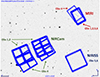 |
Fig. 1. Footprint of all observations obtained in GTO programme 1283 overlaid on DSS greyscale image (from APT/Aladin). To the upper right, the MIRI pointings for Observation 1, 2, 5, 6 (thicker rectangle) and 4 (rotated 10° anti-clockwise and offset ≈ 34″ towards the north-east) are shown. The Lyot region of the MIRI imager is not shown. The parallel fields for NIRISS (P3; Obs 5 and 6) and NIRCam (P2; Obs 1, 2 and 4) are indicated. Obs 4 was obtained at a different position angle due to JWST safing events making the schedule slip. |
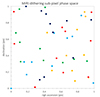 |
Fig. 2. MIRI imaging subpixel phase space sampling near detector centre, where the different colours refer to the different observations (1, 2, 4, 5, 6). The x axis shows |frac(xi − x1)| (i.e. the fractional pixel shift of the i’th dither position with respect to the 1st dither position in Obs 1) and the corresponding quantity on the y axis. The pixel scale for MIRI is 0.11″/pixel. |
For context and comparison, we show in Fig. 3 the MIDIS F560W footprint (orange shade) compared to the larger area, but shallower (exposure depth ranging from 0.65 ks in F560W to 2.2 ks in F2100W) multi-filter MIRI imaging survey SMILES (programme 1207 Rieke et al. 2024; Alberts et al. 2014) and the borders of the NIRCam primary imaging area of the JADES survey (Rieke et al. 2023; Eisenstein et al. 2023a).
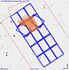 |
Fig. 3. Footprint of MIDIS MIRI imaging (orange shade) compared to the shallower SMILES survey area (blue). The dotted red lines outline the approximative border of the JADES NIRCam primary imaging field (Eisenstein et al. 2023a). |
In Fig. 4 we show the resulting image (see Section 3) and exposure map for the mosaic of all F560W observations. Due to the use of different pointings and PAs the mosaic boundary has a complex shape. For convenience in characterising the varying depth over the field of MIDIS, we define regions of approximately equal depth:
-
A (deepest, yellow) defined by the overlapping regions of the MIRI imaging field formed by Obs 1–2, 4 and 5–6, where the exposure time is 37–41.3 h.
-
B (deep, green) where the exposure time is ≥24 h. This also includes the Lyot region for Obs 1–2 and 5–6 and with partial overlap from Obs 4. The depth in the Lyot region is non-uniform due to the occulting mask and supporting instrument struts.
-
C (NE extension, purple) mainly represents the area of Obs 4 which does not have overlapping observations from Obs 1–2, 5–6, and where the total exposure time amounts to ≥7 h.
-
In the area outside of these regions (the ‘external’ region) the depth varies due to partially overlapping dither positions and ranges from ∼1 (very small area) to ∼6 hours.
The NIRCam and NIRISS parallel observations will be described in forthcoming papers. Some results from the NIRCam parallels have already be published (Perez-Gonzalez et al. 2023; Caputi et al. 2024) and more are in preparation.
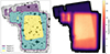 |
Fig. 4. Left: F560W image with linear intensity scaling. Coloured patches show regions with different depths where we have estimated the noise (see Table 1): the deepest area (A), where Obs 1–2, 4–6 overlap (yellow). The deep area (B), where Obs 4 does not overlap fully with the others (green). Outside these areas, there is coverage at less depth, notably the NE extension which only has observations from Obs 4. The area with at least 7h of combined integration is denoted C (purple). The orientation is in the detector plane (x,y). Right: Exposure time map. |
3. Reductions and calibration
Three different groups within the team made independent reductions to allow for cross-validation of the final images and photometry. The data were first reduced and calibrated with the JWST pipeline. This produced images with residual stripes and residual background (Morrison et al. 2023; Dicken et al. 2006). We adopted different schemes designed to counter these effects while not distorting the photometric calibration (defining our ‘customised’ pipeline, see below). In addition, we applied an iterative masking of sources for the background estimation: sources appearing after the first run were masked, and then the background was refitted masking new sources that appeared; in total, three passes were done.
After careful vetting of the resulting mosaics from the three groups, they showed a very good overall photometric agreement, and were found to be largely equivalent. We adopted the version giving the most homogeneous background for our first internal release (v1.4), described below.
The adopted mosaic was reduced with the JWST pipeline version 1.12.3, pmap 1137, with several customised reduction steps especially developed for these data which we here describe (see also Perez-Gonzalez et al. 2024a, and references therein): The MIRI F560W data present several artefacts that affect the homogeneity of the background, including a vertical (and a dimmer horizontal) striping (most prominent in the bottom quarter of the detector) and diffuse localised emission linked to cosmic ray showers. To cope with the former, after stage 1 and stage 2 of the JWST pipeline, a master super-background image was constructed for each one of the 96 exposures taken by MIDIS, using the median of the rest of the images obtained at different different dither positions to homogenise the background for a given exposure. The background patterns were found to be temporarily variable, so we restricted the data to be used to correct a given exposure to images taken within a week. For the MIDIS dataset, this translated to completely independent super-background frames for the 2–6 December (Obs 1–2, 5–6) and 20 December (Obs 4) datasets. Before the median calculation, sources detected in an initial run of the JWST pipeline were masked in each individual exposure. This was done after correcting the WCS, which typically present 0.2″–0.6″offsets in the raw data compared to the final mosaics whose WCS is calibrated with Gaia star positions. Before producing the final superbackground image, all frames were homogenised to the same median background of the image that was corrected for background inhomogeneity. The effect of cosmic ray showers was partially taken into account by the JWST pipeline, but they are not totally corrected and this is still a significant contributor to the noise in the final mosaic. Our bespoke method also included a row and column median-filtering and a smooth (100 × 100 pixel2) background subtraction to completely flatten the background accounting for very diffuse cosmic ray showers that are not handled by the pipeline. These additional processing steps applied to the JWST pipeline define our customised pipeline.
Summary of noise and depth measurements.
After the background was homogenised, we calibrated the WCS of each stage 2 image using the tweakreg external routine provided by the CEERS collaboration (Bagley et al. 2023), using the Hubble Legacy Field catalogue (Whitaker et al. 2019) as the reference. Finally, all images were stacked using the JWST pipeline’s stage 3.
The final output image was drizzled to different pixel scales: 0.11″ (nominal MIRI pixel scale), 0.06″ for robust MIRI only applications, and also 0.03″ and 0.04″ for various comparisons with NIRCam and HST data. For the finer pixel scale mosaics, we note that they may suffer from insufficient sampling in the external region. In Fig. 4 we show the resulting F560W image and the corresponding exposure map. Figure 5 shows a RGB composite with F560W in red, NIRCam/F356W in green, and F150W in blue, where the white contour outlines the limits of MIDIS (and outside of these limits the colours of galaxies appear blueish/greenish due to the missing red channel). In the same figure, the footprints of deep MUSE (blue, Bacon et al. 2023) and ALMA (red, for details see Boogaard et al. 2024) surveys are shown.
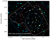 |
Fig. 5. RGB composite of the MIDIS field, with its boundaries outlined by the white contours (the irregular shape of the field is due to the use of two different pointings/PAs and that the nominal FOV has an extra square at the top left where the Lyot coronograph is located). The F560W filter is shown in red, NIRCam F356W in green, and F150W in blue (the latter two from JADES, Rieke et al. 2023). We note that the sources outside the white contour appear blueish/greenish due to the lack of MIRI data there. The thin blue contours outline deep MUSE spectroscopic surveys at 10 h and 30 h (large and small squares) and the MUSE eXtreme Deep Field (MXDF, circle) reaching up to 140 h (Bacon et al. 2023), and the red contour outlines the extent of the deep ALMA data from ASPECS at 1.2 mm and 3 mm (see Boogaard et al. 2024 for details). |
3.1. Noise measurements and pixel correlation
In order to determine the depth of the observations, we need to measure the background noise in our images on scales comparable to our detected sources. The noise levels are, in addition to the source size, affected by the photometric zeropoint and an aperture correction which in turn depends on the encircled energy distribution of the PSF.
In Fig. 6, we show how the background sky noise, measured on blank sky in 0.45″ diameter apertures, scales with exposure time for our superbackground calibration (customised pipeline) and the nominal JWST pipeline output, showing the former to scale as  , (where t is the exposure time), while the latter shows a much more modest decrease in the sky noise with t. This figure illustrates the improvement in background noise for our data customised pipeline reduction compared to the nominal JWST one.
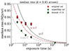 |
Fig. 6. Sky noise vs exposure time for the JWST pipeline output (red) and our customised pipeline including a super-background calibration (green). We stress that these have not been corrected for correlated noise induced by the drizzling procedure. The curves show different scalings of the RMS vs exposure time, but are not fits to the data. |
The sub-pixel dithering and resampling in the drizzling procedure means that the output pixel fluxes become correlated, which artificially lowers the pixel-to-pixel RMS background noise in the output image (as it would in a box-car smoothing). These effects have been thoroughly discussed in Fruchter & Hook (2002); and as we have many dither positions uniformly filling the sub-pixel phase space (see Fig. 2), their equations 9 and 10 for calculating the scaling, R, with which the RMS should be multiplied, are expected to be directly applicable to our data.
We produced drizzled image mosaics of different scales (s = sout/sin, i.e. the output over nominal pixel scale) and pixfracp ∈ [1, 0.9, 0.7, 0.5, 0.0], enabling us to directly test the effect of pixel correlation on the background noise. For our nominal image mosaics with pixfrac p = 1, and scale 0.11″ (s = 1, i.e. native scale), 0.06″ (s = 0.545), 0.04″ (s = 0.36), and 0.03″ (s = 0.27), the noise correction factor that should be applied to the background noise is predicted to be R = 1.5, 2.24, 3.13 and 4.03, respectively.
There are different ways commonly employed to measure the background/sky noise in reduced images. For point sources (or quasi-point sources such as very faint galaxies), it is customary to perform aperture photometry, in an aperture with diameter dap. An aperture placed on blank sky will contain pixel values with a RMS of σpix. One can then take the average or median of the standard deviations measured in such apertures as ⟨σpix⟩; we here adopt the median, being more robust.
The 1σ sky noise, which we denote σmedpix is then obtained by multiplying ⟨σpix⟩ with  (where Npix = π(dap/2sout)2 is the number of pixels in the aperture), and the correlation factor R above:
 (1)
(1)
For this purpose, we first made a segmentation map, masking out regions with bright emission, and placed random apertures in the remaining area, while rejecting those that contain detected faint sources. We did this measurement in 1000 randomly drawn apertures for mosaics generated with different pixfrac applying the correction (R) for correlated noise, and arrived at close to identical estimates for ⟨σpix⟩. Hence, the formulae of Fruchter & Hook (2002) accurately describes the effect of noise correlation when varying pixfrac in our dataset.
Another commonly used method, which to some extent mitigates the effect of pixel correlation, is to take the standard deviation (𝒮) of the total flux, fap, in apertures placed on blank sky close to an object:
 (2)
(2)
where Rap accounts for the correlation between aperture fluxes (referred to as ‘block sum’ in Fruchter & Hook 2002, Rap ≪ R). For a flat background of random noise, these two methods are identical. However, if the background is not perfectly flat over the image, σaper will be inflated. This does not affect the σmedpix method because that measure uses the median of local noise estimates.
In our final image (v1.4), the low spatial frequency variations of the background have been removed by the superbackground subtraction, but our tests show that σaper is lower when measured semi locally (over regions smaller than 10″ × 10″) than globally by ∼30%, while σmedpix remains constant, showing that the background subtraction, as expected, is not perfect and that small/medium spatial scale variations remain. However, when looking at the standard deviation of all pixels within the sky apertures (defined as σpix) we find a sky noise which is constant with aperture size and much closer to the σmedpix estimate. This reflects that the background variation on pixel to pixel scales is not very strong (but still causing the slightly higher noise level). The agreement between σpix and σmedpix is good for dap = 0.45″, with the former being marginally larger which we attribute to the remaining small scale background variation. In Fig. 7 we compare the noise measurements described above. The right-hand panel shows that the sky noise (here per pixel) is roughly constant with aperture size, except for σaper.
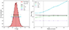 |
Fig. 7. Left panel: Flux distribution of all pixels within the sky apertures (see text). The distribution closely follows a normal distribution, showcasing that our method of selecting sky apertures is robust. The black error bar shows the observed standard deviation of the distribution, and the other bars show different noise estimates. The shaded extensions to the bars show the effect of applying the drizzle correlation factor (R and Rap, for σmedpix, and σaper, respectively). Comparing the extended green bar to the extended cyan bar then give very similar results. The black bar, gives the total statistics for all the pixels contained within our apertures. The purple bar shows the noise as inferred from the image error extension (σERR). Right panel: The effect of aperture size on the noise estimates. We use an aperture radius of 0 |

We finally compared our noise measurements to those provided by the error extension from the pipeline and found that the latter generally underestimates the true background noise1. The difference is smallest (and negligible) when employing s = 1 and p = 0, but increases for smaller pixel scales (s) and p > 0. We estimate the error extension noise (σERR) by measuring the average variance inside the sky apertures.
For the case s < 1, p > 0 we find that the ratio Rerr = σmedpix/σERR by which the error frame underestimates the noise increases with the aperture size, but is largely constant for rap ≥ 0.225 (i.e. ∼ two native MIRI pixels) and amounts to Rerr = 1.72 for 0.06″ (s = 0.545, p = 1) and Rerr = 2.5 for 0.04″ (s = 0.36, p = 1). Given that 1 < Rerr < R, we conclude that the error frames from the JWST pipeline (version 1.12.3) to some extent but not fully account for the pixel correlation introduced by subpixel dithering and drizzling in MIRI, and should not be taken at face value.
3.2. Photometric depth
For the output mosaic with pixel scale 0.06″ the measured 5σ average sky noise for dap = 0.45″ and using the σmedpix method is 29.33 mag (1σ is 31.08 mag) in the deepest area (A). For a point source in a dap = 0.45″ aperture, the encircled energy fraction is 0.53, and hence our sky noise corresponds to a 5σ limiting point source magnitude of 28.65. However, given the large variations in the exposure time, we provide in Table 1 also the depth for areas B (28.5 mag) and C (27.7 mag) and the combined A+B area (28.6 mag). For the external area, the net exposure times vary even more, introducing larger variations in depth, but 27 mag can be taken as a representative value for the 5σ point source limit (see Table 1).
In Fig. 8, we show the variation in RMS sky noise (left) and resulting point source limiting magnitude (right). In making these maps, regions with sources have been interpolated over.
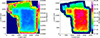 |
Fig. 8. RMS (left) and depth (right) map for output scale of 0.06″/pixel. |
Our resulting point source depths can be compared to the prediction from the exposure time calculator which currently gives 28.31 mag for a 40 h exposure (relevant for area A) in low background conditions (and with background measured in a r = 0.5″ − 1.5″ annulus). Hence, we are out-performing the ETC by ∼0.35 mag. Improvements in the measured vs predicted depth of MIRI was found also in the SMILES survey (Alberts et al. 2014). Currently, the understanding and correction of cosmic ray showers is still developing23. It is not unlikely that a future improved handling of the cosmic ray showers could improve the depth of the MIRI Deep Survey even further.
Finally, we note that the background noise and point source limiting magnitudes also depend on the pixel scale adopted. The above measurements are for 0.06″ and the same values are found for 0.11″ (native MIRI pixel scale), while for the 0.04″ and 0.03″ scales, the images are ∼0.05 magnitudes shallower.
4. Ancillary data
For a characterisation of the sources we make use of ancillary data of the HUDF/XDF area from HST (Illingworth et al. 2013), JWST: JEMS (Williams et al. 2004), FRESCO (Oesch et al. 2023) and JADES (Rieke et al. 2023). In addition we made use of published Spitzer/IRAC3 photometry (Stefanon et al. 2021). We also made use of the DAWN JWST Archive (DJA4) that coherently reduces, process and combines all public JWST observations using the GRIZLI pipeline (Brammer 2024). To enable multi-wavelength, multi-instrument analysis, the DJA mosaics are drizzled to a pixel scale of 0.04″ and aligned to GAIA DR3 (Valentino et al. 2023; Gillman et al. 2023, 2024). In accompanying papers we do, in addition, compare the MIRI results to available data from X-rays (Gillman et al. 2025), ALMA (Boogaard et al. 2024) and MUSE (Iani et al. 2024). We note that Fig. 5 is zoomed in on MIDIS which is fully encompassed by the wider area JADES and Spitzer surveys of the region (see also Fig. 3).
5. Photometry and source extraction
We have performed source detection with python/sep (Barbary et al. 2016) and basic aperture photometry with python/photutils (Bradley et al. 2024). In addition we present model based photometry based on THE FARMER (Weaver et al. 2023), which incorporates the effect of a varying PSF full width at half maximum (FWHM) for different filters in HST, NIRCam and MIRI.
5.1. Source detection and basic photometry
Source detection in the nominal 60 mas F560W image was done using sep (Barbary et al. 2016), a python wrapper for Source Extractor (Bertin & Arnouts 1996). In Table 2 we give the extraction parameters used for the catalogue presented in this paper. We used the error maps from the JWST pipeline (scaled by a factor 1.7 to account for the noise underestimate in these maps, see Section 3.1) multiplied by the threshfloat parameter as the pixel detection threshold. As a first control of the detection, we applied a a SNR limit of 2 (2σ, Δmag < 0.5) estimated within the source segment (from the detection segmentation map). With these parameters and SNR rejection we find 2571 sources. Given that this is a single filter detection a large number of the faint sources are expected to be spurious, even when filtering the image before detection. We thus manually inspected the sources, rejecting 170 sources that are obviously spurious (single hot pixels, cosmic ray artefacts, PSF features and some sources near the detector edges) and arrive at a final object list containing 2401 sources.
Source detection parameters.
We estimated the number of spurious sources by running the same detection on an inverted F560W image and applying the same SNR rejection. We also adjusted the spurious detection rate for the manual inspection. The rate of spurious detections in our final catalogue is 24% (of 2571 sources), which is higher than expected given the SNR cut applied. Hence, in addition to the 170 manually rejected sources, there are likely ∼400 spurious sources remaining, many of which will be ≲5σ sources, and the number of true sources is likely ≈2000. However, in this first single band catalogue for the deep MIRI data we have elected to be liberal in including sources (both in setting the detection parameters and in the manual inspection). Care should therefore be taken when using this catalogue, and multiple filters (e.g. NIRCAM data or other MIRI filters) should be used for any further characterisation of the sources. It should be noted that if we apply a more aggressive SNR cut the spurious rate naturally goes down, at SNR > 10 the rate is 2%. Why the spurious detection rate is higher than expected is hard to explain but a likely explanation could be image defects that remain in the stacked image due to problems with outlier (in particular cosmic ray) rejection. As the JWST pipeline improves in future releases, it is likely that the number of spurious sources will decrease. In Perez-Gonzalez et al. (2024b) and Jermann et al. (in prep.) we describe methods (based on investigating and rejecting individual frames) that can be used to verify that interesting sources are real, even with single filter detection. We note that the number of F560W > 2σ sources with a counterpart in the JADES catalogue is 1879.
Photometry was obtained for the detected sources using photutils and two different apertures: (i) circular apertures with a radius of 0.2″, and (ii) Kron apertures (Kron 1980). While the Kron apertures provides an estimate of the total flux of the sources, the small circular apertures will show smaller statistical errors with the caveat that not all of the flux is included. We aperture correct the circular aperture photometry using our PSF model (Boogaard et al. 2024). In Fig. 9 we display the resulting Kron aperture photometry for MIDIS.
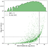 |
Fig. 9. Top: F560W number counts for Kron magnitudes. Bottom: F560W Kron magnitudes vs photometric uncertainty. The derived 5σ point source limiting magnitude is indicated by the dashed vertical line. |
5.2. Farmer photometry
Multi-wavelength (MIRI, NIRCam and HST) photometry was derived for all sources detected in the 0.04″ v1.4 F560W image with THE FARMER software (Weaver et al. 2023). THE FARMER simultaneously models all detected sources using parametric models, allowing accurate deblending of crowded fields and multi-wavelength datasets with varying resolutions. We opt for the 0.04″ F560W image to match with the images available in the DAWN JWST Archive (see Sect. 4).
In brief, we first detected and modelled the galaxies in F560W MIRI band using our F560W PSF model (Boogaard et al. 2024). We then performed forced photometry in the other multi-wavelength bands, using the WEBBPSF models for NIRCam (Perrin et al. 2012, 2014), allowing for the flux to vary, whilst keeping the structural parameters fixed (details will be presented in Gillman et al., in prep.).
5.3. Comparison with Spitzer/IRAC
We have compared our F560W photometry to that of Spitzer/IRAC channel 3, which has a similar bandpass to F560W, for the HUDF (Guo et al. 2013; Stefanon et al. 2021). In Fig. 10 we show a comparison of our F560W photometry (measured with FARMER) and IRAC/Ch3. For fluxes F ≲ 10 μJy we find very small flux differences consistent within the large photometric errors of the Spitzer/IRAC observations. At bright fluxes F ≳ 20 μJy, we see a gradual systematic brightening of IRAC vs MIRI, amounting to ≳20% at the bright end. Either the Spitzer fluxes are too large, or the MIRI ones too small. The number of sources in the bright end is naturally small; nevertheless, we speculate on possible explanations for this offset in the next paragraph.
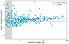 |
Fig. 10. Comparison of MIRI/F560W to IRAC/Ch3 photometry. For < 15 μJy the fluxes agree, while for > 20 μJy the IRAC photometry is systematically brighter. |
The Spitzer catalogue of Guo et al. (2013) contains matched photometry derived by determining the source position, size, and shape from the HST/F160W filter; matching the source shape to IRAC using the PSF, and finding the IRAC flux by fitting the convolved source model to the IRAC data. This is similar to the method used in FARMER, but for our photometry the morphology comes from the F560W image itself. In contrast, IRAC/Ch3 samples a factor of 3.5 longer wavelengths than the HST/F160W filter from which the source model was made. Most of the bright sources are at low (z < 1) redshift, meaning that HST/F160W samples λrest ≳ 8000 Å while IRAC/Ch3 samples λrest ≳ 2.9 μm. If the size (e.g. the effective radius) or shape of the source varies with λ, this may give highly uncertain flux measurements, in particular for sources that are faint in the HST/F160W image, but bright in the mid-IR. In addition, for this redshift range, systematic offsets might be present if galaxies at a given brightness have consistently different morphologies between the rest-frame wavelengths probed by HST/F160W and IRAC/Ch3.
In addition to the FARMER photometry comparison we have also compared the IRAC measurements to photometry from photutils using large Kron apertures which show the same offset in the bright end. A more detailed investigation into this effect is outside the scope of this work, but we note that the MIRI/F560W photometry is obtained directly in high-resolution images and will thus give less model-dependent photometry.
We note that discrepant results for some bright sources were found also for JADES when comparing IRAC/Ch2 to F444W (Rieke et al. 2023), and in CEERS for MIRI/F560W and F770W (Yang et al. 2023), and for other MIRI/F560W fields (Sajkov et al. 2024). At least partly, this can be attributed to source blending in the Spitzer data due to its order of magnitude broader PSF, an effect which is also present in the comparison for our data.
In Fig. 11, we show a comparison of our MIRI/F560W 5.6 μm image to the Spitzer/IRAC/Ch3 5.8 μm image (cropped to the size of the F560W image). The maximum depth of the Spitzer image is ∼40 hours reaching 25.6 mag (at 1σ, Stefanon et al. 2021, hence 5σ is ∼24 mag). The increase in resolution (a factor of ∼15) and depth (close to 5 magnitudes) despite the same exposure time is quite apparent.
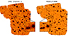 |
Fig. 11. Left: Spitzer/IRAC band 3 (λeff = 5.8 μm), based on exposure time of ∼40 h, cropped to the size of the MIDIS field. Right: our MIRI/F560W image. The insets show a zoom-in on a 12″ × 12″ region highlighting the improvement in sensitivity and resolution. |
6. Photometric redshifts
Photometric redshifts were derived from the multi-wavelength FARMER fluxes for each source using the EAZY software (Brammer et al. 2008). We used thirteen templates from the Flexible Stellar Populations Synthesis code (FSPS; Conroy & Gunn 2010) described in Kokorev et al. (2022) linearly combined to allow for maximum flexibility. The included spectroscopic redshifts are from the literature: the MUSE Hubble Ultra Deep Survey (Bacon et al. 2023), 3DHST (Brammer et al. 2012; Momcheva et al. 2016), and the JWST Advanced Deep Extragalactic Survey (JADES: Bunker et al. 2024; D’Eugenio et al. 2024).
While spectroscopic redshifts have been obtained for many galaxies in the XDF, both before and with JWST, photometric redshifts provide a more complete picture of the z-distribution, and to fainter flux levels. Photometric redshifts based on NIRCam photometry alone are expected to be quite secure, especially for star-forming systems based on the good coverage of the rest frame UV and the Lyα break up to z ≳ 10. The power of MIRI is primarily to probe the rest frame optical and NIR for a more secure determination of the stellar population and identification of intrinsically red, for example dusty, sources. Nevertheless, it is interesting to investigate how the addition of MIRI affects the photo-z solution.
From the results of EAZY we analysed the systematic offsets between the observed and fitted SED to find a suggested zeropoint (ZP) error of ΔZP = −0.0388. This is smaller than the median absolute offset for both NIRCam and HST filters. Hence, the MIRI calibration is from this comparison fully consistent with that of NIRCam, and suggests that the MIRI zero point is accurate. Moreover, we see no dependence of ΔZP for F560W with source brightness, suggesting that the offsets with respect to IRAC/Ch3 likely is due to the IRAC photometry rather than MIRI.
In Fig. 12, we show the comparison of spectroscopic redshifts to photometric redshifts based on FARMER/EAZY. In total, we find 581 sources with spectroscopic redshifts and F560W photometric uncertainties better than 2σ within our field of view. We then define the redshift uncertainty as:
 (3)
(3)
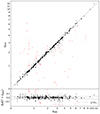 |
Fig. 12. Upper panel: Photometric vs spectroscopic redshifts from the FARMER photometry and the EAZY code. The red points are outliers (> 3σz). Lower panel: Normalised difference of the redshifts (with Δz = zphot − zspec) vs spectroscopic redshift. The standard deviation of the normalised difference is σz = 0.032 with the outliers removed. |
and classify all sources with |δz| > 3σz as outliers (catastrophic failures). The fraction of catastrophic failures (shown as red circles in the figure) is 10% and the uncertainty for the remainder is σz = 0.032. Applying the same method to a comparison of the JADES (data release 2, Eisenstein et al. 2023b) photometric redshifts to the spectroscopic redshifts we find a similar uncertainty and catastrophic failure fraction. As expected the addition of F560W data does not improve the photometric redshift estimates over the full sample (but see Sect. 7.5).
In Fig. 13, we show the redshift distribution vs F560W magnitude. This figure includes, in addition to each source with a spectro-z (in red), photometric redshifts (in blue) for all galaxies (1069) for which the photo-z uncertainty Δz < 1. Another ∼1000 sources have Δz > 1, and have zph distributed from ∼0 to ∼18, with the majority at zph > 6 and with peaks at z ∼ 0.6, 4.5 and 12. While the individual redshifts of those are to be regarded as uncertain, a significant fraction is likely to be at z > 6. Finally, there are ∼500 sources with no phot-z solution at all from EAZY, many of which are likely to be spurious sources (see Section 5.1).
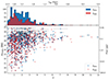 |
Fig. 13. Top: Histogram showing spectroscopic (red) and photometric (blue) redshift distribution. Bottom: Spectroscopic (red) and photometric (blue) redshift vs F560W magnitude. The photometric redshifts are estimated with EAZY. Only sources detected at σ > 2 in F560W, and with a 1σ redshift uncertainty Δz < 1 were included (1069 sources). |
7. Results
The final MIRI image is shown in Fig. 5. As was described above, the photometric analysis shows that we reach a 5σ point source depth of 28.6 mag (AB), and that this is significantly deeper than the pre-launch and ETC estimates (∼28.3). This demonstrates the spectacularly successful realisation of JWST (Gardner et al. 2023) and MIRI (Wright et al. 2023).
We show in Fig. 9 the resulting F560W magnitude distribution for the 2401 sources (but we note that there are likely spurious sources remaining, especially at > 28 mag, see Sect.5.1). In Fig. 14 we show the F560W mag vs F356W–F560W colour for matched sources with ≥5σ in F560W and ≥2σ in F356W from JADES. For 1.5 < z < 10, F560W probes the rest frame K-band (2.2 μm) to visual (0.5 μm) while NIRCam/F356W probes the rest frame ∼H-band (1.6 μm) to the ∼U band (0.32 μm). Hence this colour gives an indication of diversity of stellar populations present in the sample. Since sources are detected in both filters, and visually inspected, the spurious fraction should be very small, though likely not null.
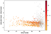 |
Fig. 14. F560W magnitude vs NIRCAM/F356W–F560W colour. Only sources with a F560W (F356W) magnitude uncertainty of 0.2 (0.5) or lower are included. The black circle indicates a confirmed MERO currently under investigation (Jermann et al., in prep.). The yellow–to–red colour scale indicate photometric redshift of the sources (grey, smaller, points do not have a valid redshift estimate). |
7.1. Number counts
Fig. 9 (upper panel) shows the number of sources per 0.2 magnitude bin derived from the total MIRI image. The distribution peaks at ∼27 mag where it is rather flat and then turns down for > 28 mag due to increasing incompleteness (varying over areas of different depth, see Fig. 4 and Table 1). Our peak counts at ∼27 mag are ∼90 mag−1 arcmin−2 (3.4 ⋅ 105 per magnitude and □°), which can be compared to Spitzer/Irac/Ch3 finding a factor of ∼15 lower surface density at ∼21 AB magnitudes (Fazio et al. 2004b, converted from a Vega magnitude of 17.3). Our counts at the same brightness suffer from low numbers given the small area of MIDIS but are at 4.8 ± 1.1 mag−1 arcmin−2 consistent with Spitzer finding 5.5 and 6.5 mag−1 arcmin−2 in two different fields.
For comparison, the F560W counts in CEERS (Yang et al. 2023) and SMILES (Stone et al. 2024) extend to ∼26 and ∼25.6 magnitudes, respectively. Deeper F560W counts were presented by Sajkov et al. (2024), based on 8 fields with exposure depth of 1.85 h per field, reaching ∼100% completeness at 0.1 μJy (26.4 mag) and a surface density for 0.09 μJy of 5.1 ± 0.6 ⋅ 105 per square degree. This limit is brighter than what we get in the external area (outside of region C) where the 5σ photometric limit is typically ≳27 or > 0.05 μJy (see Fig. 8 and Table 2). Hence our total MIDIS area should be representative to 0.1 μJy at ≳10σ with high completeness and with an insignificant number of spurious sources. We find (see Fig. 15) 856 sources down to 0.09 μJy, over a total area of 4.711 square arcmin or 6.54 ± 0.22 ⋅ 105 per square degree (where the uncertainty quoted is the 1σ Poisson error), hence consistent within 2σ but suggesting that XDF is perhaps somewhat overdense at 5.6 μm. The total density of sources with F560W magnitude ≤27 (0.58 μJy, where we are reasonably complete over the full area) is 9.6 ⋅ 105 per square degree. Pushing the counts to fainter limits (≲0.02 μJy) over areas A+B would require a more careful rejection of spurious sources which can be accomplished by including photometry from JADES and the upcoming deep F770W and F1000W imaging of XDF from JWST GO programme 6511.
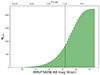 |
Fig. 15. F560W cumulative number counts for Kron magnitudes. The vertical dashed line indicates a flux limit of 0.10 μJy as in Sajkov et al. (2024). |
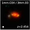 |
Fig. 16. Example of galaxy at cosmic noon (z ∼ 2.5) as seen in MIRI/F560W (red), NIRCam/F182M (green) and HST/F814W (blue) from Boogaard et al. (2024). The MIRI emission unveils the presence of a disc-like stellar mass distribution, while the NIRCam and HST images highlight young star forming regions. The cutout is 4″ × 4″ (corresponding to ∼3 × 3 kpc). The FWHM (0.207″) of the MIRI/F560W PSF is shown as a white circle in the lower left. |
7.2. Redshift distribution
As mentioned above, and shown in Fig. 12, for 90% of the 581 sources with F560W photometry above the 2σ level and available spectroscopic redshifts, the agreement with the photo-z derived from EAZY is very good (σz ≈ 0.03, see Sect. 6 and Eq. (3)). In Fig. 13, we show the distribution of spectroscopic and photometric redshifts versus F560W magnitude. For the photo-z estimates we have only included sources with F560W fluxes > 2σ and and with a 1σ redshift uncertainty Δz < 1, in total 1075 sources. While the selection functions for spectroscopic and photometric redshifts are different, they span a similar range, as shown in the histogram on top.
The bulk of MIRI/F560W sources with determined redshifts are at z < 4, but there is still a good number (74) of sources at 4 < z < 8. For z > 8 the distribution thins out, with 3 objects at zphot ∼ 10 − 12, among them JADES-GS-z11-0 (see Sect. 7.5). These sources all have F560W magnitudes close to 27. There is a large number of fainter MIRI sources (up to 29th magnitude) with high-redshift (zphot > 6) solutions but larger uncertainties (and the NIRCam photometric uncertainties are also larger for such, rendering the photo-z uncertainty being Δz > 1), and while uncertain a large fraction of these are expected to be at z > 6.
This demonstrates the ability of MIRI to detect galaxies in the EoR, at z > 6, but requires reaching depths of > 27 magnitude in F560W. As NIRSPEC campaigns on the HUDF progress, an increased number of MIRI 5.6 μm sources with spectroscopic redshifts will likely emerge, and with deeper NIRCam images being obtained, also many fainter F560W sources will eventually get a reliable photo-z.
7.3. Morphologies
The FWHM of the MIRI PSF in F560W is 0.207″, corresponding to 1.4 kpc at z = 4. By tracing redder rest frame wavelengths (λrest > 1 μm at z < 4.6) than NIRCam, and with superior resolution and sensitivity compared to Spitzer and WISE, MIRI has a great potential for characterising the stellar mass distribution of high-redshift galaxies. In Fig. 16 we show an example of a galaxy at z = 2.454, also detected in CO and continuum with ALMA (Boogaard et al. 2024) with MIRI/F560W in red, NIRCam/F182M in green and HST/F814W in blue. Here, the MIRI emission (rest frame 1.6 μm) shown in red clearly traces an ellipsoidal shape indicative of an inclined disc, while the bluer filters (probing UV/visual) highlight (in yellow/green) smaller localised star-forming regions (for more galaxies and details, see Boogaard et al. 2024, where black/white single filter snapshots of individual galaxies also demonstrate this).
Several studies utilising the power of MIDIS to unveil the morphology of high-redshift galaxies are underway (Costantin et al. 2024; Gillman et al., in prep.; Moutard et al., in prep.). Another example is a study of X-ray detected AGN candidates (Gillman et al. 2025).
7.4. MIRI red sources
As can be seen from Fig. 14 most sources form a broad sequence of F356W–F560W ≈ − 0.15 ± 0.6, but there are also > 100 sources with much redder colours, > 1. We find in addition a similar number of red sources with upper (1σ) limits in F356W, which are in most cases previously unknown (i.e. not catalogued in JADES). Given that the F560W image still likely contains a significant number of spurious detections, sources with upper limits in F356W are not included in Fig. 14 and we do not discuss them further here. Sources with detections in both F560W and F356W are more secure.
We characterise the expected F356W–F560W colours of stellar populations of various age at different redshifts with the Yggdrasil spectral synthesis model5 (Zackrisson et al. 2011) using an instantaneous burst model with metallicity Z = 0.004 and Kroupa initial mass function. We find that unreddened stellar populations with age < 1 Gyr would for z ≤ 10 not be expected to show F560W–F356W colours larger than 1.4, and for young populations (age ≤ 30 Myr) colours of < 0.1 for z < 5 and < 0.5 for z ≤ 10 are expected. At z = 3 an extinction of AV = 5 would add 1.4 magnitude in colour; and at z = 8, AV = 2 would add 1 magnitude in colour (assuming the attenuation law of Calzetti et al. 2000). Hence a source with F356W–F560W > 1.5 could either be a high-z quenched galaxy (with a predominantly old population), or a young (starburst) significantly reddened source with AV > 5 at z ∼ 3 or AV > 2 at z ∼ 8. We term such objects ‘MIRI extremely red object’ (MEROs). We note that already F356W–F560W > 1 would require AV > 3 for a ≤30 Myr stellar population at z = 3 and AV > 1 for z = 8; or alternatively a > 300 Myr old population at z > 8, and such objects are termed ‘MIRI red objects’ (MROs). These colour criteria do not consider Galactic brown dwarf stars, which are rare but can have very red colours (Langeroodi & Hjorth 2023), or AGN. Of relevance for the latter class, JWST has discovered a population of red compact sources (e.g. Barro et al. 2024), termed little red dots, many of which have broad Hα line emission (Matthee et al. 2024), and red NIRCam–MIRI colours (Perez-Gonzalez et al. 2024a), and likely represent a mix of dusty AGN and dusty starbursts.
As is evident from Fig. 14, out of the ∼60 MERO candidates identifiable, only 2 sources currently have reliable photometric redshift estimates. For the similar number of MROs (with 1 < F356W–F560W < 1.5) five sources have photo-z estimates. However, most of the very red objects are also faint in F560W (∼28 ± 1.3 mag). Given the complicated nature of cosmic ray residuals in the MIRI image (see Section 5.1) we still suspect that some of these objects could be spurious (also considering their low S/N in F356W). In order to confirm these objects as real astrophysical sources a more detailed procedure is needed. Such an investigation is currently underway and will be presented in Jermann at al. (in prep.), and one of the confirmed sources is indicated with a black circle in Fig. 14. Nevertheless, sources with F356W–F560W > 1 constitute a potential treasure trove for exploring dusty/old galaxies and AGN at high-z, but requires scrutiny in assessing their reality.
Naturally, the definition of MRO/MEROs according to the above reasoning depends on the filter combination used (for instance, for F444W–F560W, the MRO criterion would be > 0.5), and could be redefined for other colour indices, and in selecting sources for further study, all available photometric data should be used. Two examples of interesting MIRI red objects identified from other bands (F1000W) in MIDIS are the Cerberus source (Perez-Gonzalez et al. 2024b) detected at 2.8σ in F356W, and at 5.9σ F1000W (with F356W–F1000W = 4.1), but undetected in F560W (upper limit 29.7, implying F356W–F560W ≲ 1.5); and the AGN candidate Virgil at z = 6.6 (Iani et al. 2023).
The cycle 3 JWST GO programme 6511 will image the XDF deeply with MIRI in F770W and F1000W. This will likely produce many more securely identified MIRI red objects.
7.5. High-redshift galaxies detected in MIDIS
In Fig. 17, we show photometric redshift fits of the eight highest redshift galaxies with a reliable photo-z estimate in our F560W selected catalogue. The fits are done with EAZY (see Section 6). We note that these are not bona fide SED fits, and use a limited grid for nebular emission, explaining why the strength of F560W (containing strong lines at these z) is not always well reproduced. The legend contains JADES id number, coordinates, JADES photo-z, our photo-z solution and its χ2, and spectroscopic redshift (available for 4 of the sources). For all but one source (second row, right column) there is a good agreement between the photometric redshifts from JADES and our estimates. The discrepant source has a z = 2.92 solution in JADES (i.e. the drop in flux shortwards of 1.5 μm was identified as a Balmer break), but the bright F560W flux rule out this solution in favour of z = 10.7 where the F560W flux is boosted by Hβ + [O III] emission. This illustrates the potential of MIRI for securing and characterising very high-redshift sources, provided faint flux levels can be reached. In Rinaldi et al. (2023) we used MIDIS F560W imaging to select 12 strong Hα emitters at z ≈ 7 − 8, and found them to have high ionising photon production efficiencies (ξion, see Rinaldi et al. 2024).
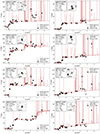 |
Fig. 17. Examples of photometric redshift fits made with EAZY for ≳8 galaxies in MIDIS. The insets show: (i) the source identification and redshift estimates; and (ii) F560W 2″ × 2″ thumbnails. The second (from top) panel on the right shows a source for which the addition of MIRI changed the photometric redshift solution from z = 2.9 to 10.7 due to the bright F560W flux being identified with Hβ + [O III]. |
The XDF contains a number of EoR candidates known from past HST imaging studies (e.g. Oesch et al. 2013, including JADES-GS-z11-0 mentioned below). The field covered by our F560W image contains two spectroscopically confirmed z > 10 sources from JADES (Robertson et al. 2023; Curtis-Lake et al. 2023): JADES-GS-z10-0 and JADES-GS-z11-0. While the former is unfortunately contaminated by a F560W PSF spike preventing its secure detection, JADES-GS-z11-0 is well detected in F560W (see Fig. 17, lower left panel, but we note that the spectroscopic redshift is somewhat lower than the displayed photo-z fit) for the first time probing the rest frame > 4300 Å emission. Notably, the galaxy is extended and presents some structure in the form of a southern extension in F560W, of which there is a hint also in NIRCam images. The extension is treated as a separate source in the JADES catalogue and has a lower (but very uncertain) photometric redshift in that catalogue. This source has recently been proposed to be a companion to JADES-GS-z11-0 (Hainline et al. 2024). The implications from the MIRI imaging will be further discussed in a forthcoming paper (Melinder et al., in prep.).
8. Summary and conclusions
Based on the MIRI European consortium GTO programme 1283, we present MIDIS (the MIRI Deep Imaging Survey) of the Hubble Ultra Deep Field, the deepest 5.6 μm image of the Universe as yet with a total integration time of 41 hours. We have processed the data with the JWST pipeline augmented by bespoke adaptations (our customised pipeline). We summarise our results as follows:
-
The deepest parts of the mosaic reach a point source 5σ limiting AB magnitude of 28.65 (12.7 nJy). This is ∼0.35 magnitudes better than the JWST exposure time calculator predicts.
-
We detect ∼2500 sources down to 2σ. Most of these (1879 sources) have counterparts at shorter wavelengths from JWST/NIRCam and the JADES survey. Due to remaining issues with the cosmic ray rejection in the JWST pipeline, we expect ∼2000 of the F560W sources to be bona fide distant galaxies.
-
Comparing the F560W photometry to Spitzer/IRAC Channel 3 observations of the HUDF, we find good agreement but we note that for sources brighter than 20.6 mag (20 μJy), IRAC fluxes are ∼20% higher.
-
There are 581 sources in MIDIS with availble spectroscopic redshifts, and for 1069 sources we could determine accurate photometric redshits (uncertainty in z < 1). For 90% of the sources with available spectroscopic redshifts, the agreement with photometric redshifts is excellent (∼3%).
-
While the majority of sources with available spectroscopic or accurate photometric redshift are at z < 4, the redshift distribution extends to z ∼ 12. Many of the sources with less accurate photomtric redshift estimates are likely to be at z > 6.
-
Number counts reveal a total density of sources ≤27 magnitudes (∼0.06 μJy) in F560W of ∼106 per square degree. Comparing to available F560W counts down to 0.09 μJy in other fields, we find the source density in MIDIS to be ∼25% higher.
-
MIDIS imaging has been demonstrated to probe the NIR rest frame morphology of galaxies out to z ∼ 4.
-
More than 100 sources have F356W–F560W colours > 1 magnitude, representing MIRI very red sources, suggesting significant dust reddening or old stellar populations at high redshift.
-
We illustrate the power of the MIDIS deep 5.6 μm survey by 8 examples of galaxies with zphot > 7, where in one case the MIRI F560W data point changes the redshift estimate from JADES from ∼3 to > 10.
Data availability
The catalogue data presented in this paper are available in electronic form at the CDS via anonymous ftp to cdsarc.cds.unistra.fr (http://cdsarc.u-strasbg.fr) or via https://cdsarc.cds.unistra.fr/viz-bin/cat/J/A+A/696/A57.
Our F560W image mosaic is made available to the community. Although the data is publicly available in the archive, the image produced by the JWST pipeline version 1.12.3 (pmap 1137) is not yet as optimised as our current reduction (with a customised pipeline). We also make the F560W catalogue used for the results presented in this paper available as a machine readable table. The catalogue includes both standard photometric properties, and model based photometry from FARMER, see Table B.1 in Appendix B.
Our data products (images and catalogues) are available at MAST as a High Level Science Product via https://doi.org/10.17909/hfg7-8j02
When improvements in the JWST pipeline and calibrations so merit, updated images and an updated catalogue will be uploaded.
We note that the effects of our custom scripts added to the JWST pipeline have not been fully propagated into the error extension. Since the JWST pipeline gives larger background noise, the error extension would underestimate the true error even more.
Acknowledgments
We dedicate this paper to the memory of our deceased and much valued MIRI-EC team members Hans Ulrik Nørgaard-Nielsen and Olivier Le Fèvre, both of whom played a central role in defining the MIDIS project. This work is based on observations made with the NASA/ESA/CSA James Webb Space Telescope. The work presented is the effort of the entire MIRI team and the enthusiasm within the MIRI partnership is a significant factor in its success. The following National and International Funding Agencies funded and supported the MIRI development: NASA; ESA; Belgian Science Policy Office (BELSPO); Centre Nationale d’Etudes Spatiales (CNES); Danish National Space Centre; Deutsches Zentrum fur Luftund Raumfahrt (DLR); Enterprise Ireland; Ministerio De Economia y Competividad; Netherlands Research School for Astronomy (NOVA); Netherlands Organisation for Scientific Research (NWO); Science and Technology Facilities Council; Swiss Space Office; Swedish National Space Agency (SNSA); and UK Space Agency. MIRI drew on the scientific and technical expertise of the following organizations: Ames Research Center, USA; Airbus Defence and Space, UK; CEAIrfu, Saclay, France; Centre Spatial de Liège, Belgium; Consejo Superior de Investigaciones Cientficas, Spain; Carl Zeiss Optronics, Germany; Chalmers University of Technology, Sweden; Danish Space Research Institute, Denmark; Dublin Institute for Advanced Studies, Ireland; European Space Agency, Netherlands; ETCA, Belgium; ETH Zurich, Switzerland; Goddard Space Flight Center, USA; Institute d’Astrophysique Spatiale, France; Instituto Nacional de Técnica Aeroespacial,Spain; Institute for Astronomy, Edinburgh, UK; Jet Propulsion Laboratory, USA; Laboratoire d’Astrophysique de Marseille (LAM), France; Leiden University, Netherlands; Lockheed Advanced Technology Center (USA); NOVA Opt-IR group at Dwingeloo, Netherlands; Northrop Grumman, USA; Max Planck Institut f ür Astronomie (MPIA), Heidelberg, Germany; Laboratoire d’Etudes Spatiales et d’Instrumentation en Astrophysique (LESIA), France; Paul Scherrer Institut, Switzerland; Raytheon Vision Systems, USA; RUAG Aerospace, Switzerland; Rutherford Appleton Laboratory (RAL Space), UK; Space Telescope Science Institute, USA; Stockholm University, Sweden; Toegepast- Natuurwetenschappelijk Onderzoek (TNOTPD), Netherlands; UK Astronomy Technology Centre, UK; University College London, UK; University of Amsterdam, Netherlands; University of Arizona, USA; University of Cardiff, UK; University of Cologne, Germany; University of Ghent; University of Groningen, Netherlands; University of Leicester, UK; University of Leuven, Belgium; Utah State University, USA. Additional acknowledgements related to specific grants: G.Ö., J.M. and A.B. acknowledges funding from the Swedish National Space Administration (SNSA). P.G.P.-G. acknowledges support from grant PID2022-139567NB-I00 funded by Spanish Ministerio de Ciencia e Innovación MCIN/AEI/10.13039/501100011033, FEDER Una manera de hacer Europa. This work was supported by research grants (VIL16599,VIL54489) from VILLUM FONDEN. L.C. and J.A.-M. acknowledge support by grant PIB2021-127718NB-100 from the Spanish Ministry of Science and Innovation/State Agency of Research MCIN/AEI/10.13039/501100011033 and by “ERDF A way of making Europe”. M.A. acknowledges financial support from Comunidad de Madrid under Atracción de Talento grant 2020-T2/TIC-19971. J.P.P. and T.V.T. acknowledge financial support from the UK Science and Technology Facilities Council, and the UK Space Agency. A.A.-H. acknowledges financial support from grant PID2021-124665NB-I00 funded by MCIN/AEI/10.13039/501100011033 and by “ERDF A way of making Europe”. E.I. and K.I.C. acknowledge funding from the Netherlands Research School for Astronomy (NOVA). K.I.C. acknowledges funding from the Dutch Research Council (NWO) through the award of the Vici Grant VI.C.212.036. RAM acknowledges support from the Swiss National Science Foundation (SNSF) through project grant 200020_207349. The paper uses JWST data from programme #1283, obtained from the Barbara Mikulski Archive for Space Telescopes at the Space Telescope Science Institute (STScI). For the purpose of open access, the authors have applied a Creative Commons Attribution (CC BY) licence to the Author Accepted Manuscript version arising from this submission.
References
- Alberts, S., Lyu, J., Shivaei, I., et al. 2014, ApJ, 976, 224 [Google Scholar]
- Bacon, R., Brinchmann, J., Conseil, S., et al. 2023, A&A, 670, A4 [NASA ADS] [CrossRef] [EDP Sciences] [Google Scholar]
- Bagley, M. B., Finkelstein, S. L., Koekemoer, A. M., et al. 2023, ApJ, 946, L12 [NASA ADS] [CrossRef] [Google Scholar]
- Barbary, K., Boone, K., McCully, C., et al. 2016, https://doi.org/10.5281/zenodo.159035 [Google Scholar]
- Barro, G., Perez-Gonzalez, P. G., Kocevski, D. D., et al. 2024, ApJ, 963, 128 [CrossRef] [Google Scholar]
- Becker, R. H., Fan, X., White, R. L., et al. 2001, AJ, 122, 2850 [NASA ADS] [CrossRef] [Google Scholar]
- Beckwidth, S. V. W., Stiavelli, M., & Koekemoer, A. M. 2016, AJ, 132, 1729 [Google Scholar]
- Bertin, E., & Arnouts, S. 1996, A&AS, 117, 393 [NASA ADS] [CrossRef] [EDP Sciences] [Google Scholar]
- Boogaard, L. A., Gilman, S., Melinder, J., et al. 2024, ApJ, 696, 27 [Google Scholar]
- Bosman, S. E. I., Davies, F. B., Becker, G. D., et al. 2022, MNRAS, 514, 55 [NASA ADS] [CrossRef] [Google Scholar]
- Bosman, S. E. I., Álvarez-Márquez, J., Colina, L., et al. 2024, Nat. Astron., 8, 1054 [NASA ADS] [CrossRef] [Google Scholar]
- Bouwens, R., Illingworth, G., Gonzalez, V., et al. 2010, ApJ, 725, 1587 [NASA ADS] [CrossRef] [Google Scholar]
- Bouwens, R., Illingworth, G., Oesch, P., et al. 2015, ApJ, 803, 34 [CrossRef] [Google Scholar]
- Bradley, L., Sipőcz, B., Robitaille, T., et al. 2024, https://doi.org/10.5281/zenodo.10967176 [Google Scholar]
- Brammer, G. 2024, https://doi.org/10.5281/zenodo.1146904 [Google Scholar]
- Brammer, G., van Dokkum, P., & Coppi, P. 2008, ApJ, 686, 1503 [Google Scholar]
- Brammer, G. B., van Dokkum, P. G., Franx, M., et al. 2012, ApJS, 200, 13 [Google Scholar]
- Bunker, A. J., Cameron, A. J., Curtis-Lake, E., et al. 2024, A&A, 690, A288 [NASA ADS] [CrossRef] [EDP Sciences] [Google Scholar]
- Calzetti, D., Armus, L., Bohlin, R. C., et al. 2000, ApJ, 533, 682 [NASA ADS] [CrossRef] [Google Scholar]
- Caputi, K. I., Rinaldi, P., Iani, E., et al. 2024, ApJ, 969, 159 [NASA ADS] [CrossRef] [Google Scholar]
- Casey, C. M., Kartaltepe, J. S., Drakos, N. E., et al. 2023, ApJ, 954, 31 [NASA ADS] [CrossRef] [Google Scholar]
- Colina, L., Crespo, Gomez A., Alvarez-Marquez, J., et al. 2023, A&A, 673, L6 [NASA ADS] [CrossRef] [EDP Sciences] [Google Scholar]
- Conroy, C., & Gunn, J. E. 2010, Astrophysics Source Code Library [record ascl:1010.043] [Google Scholar]
- Costantin, L., Gillman, S., Boogaard, L. A., et al. 2024, A&A, submitted [arXiv:2407.00153] [Google Scholar]
- Covelo-Paz, A., Giovinazzo, E., Oesch, P. A., et al. 2025, A&A, 694, A178 [NASA ADS] [CrossRef] [EDP Sciences] [Google Scholar]
- Curtis-Lake, E., Carniani, S., Cameron, A., et al. 2023, Nat. Astron., 7, 622 [NASA ADS] [CrossRef] [Google Scholar]
- D’Eugenio, F., Cameron, A. J., Scholtz, J., et al. 2024, ApJS, submitted [arXiv:2404.06531] [Google Scholar]
- Dicken, D., Garcia, Marin M., Shivaei, I., et al. 2006, AJ, 132, 117 [NASA ADS] [CrossRef] [Google Scholar]
- Eisenstein, D. J., Willot, C., Alberts, S., et al. 2023a, ApJS, submitted [arXiv:2306.02465] [Google Scholar]
- Eisenstein, D. J., Johnson, B. D., Robertson, B., et al. 2023b, ApJS, submitted [arXiv:2310.12340] [Google Scholar]
- Fan, X., Strauss, M. A., Becker, R. H., et al. 2006, AJ, 132, 117 [NASA ADS] [CrossRef] [Google Scholar]
- Fazio, G. G., Hora, J. L., Allen, L. E., et al. 2004a, ApJS, 154, 10 [Google Scholar]
- Fazio, G. G., Ashby, M. L. N., Barmby, P., et al. 2004b, ApJS, 154, 39 [Google Scholar]
- Fruchter, A. S., & Hook, R. N. 2002, PASP, 114, 144 [NASA ADS] [CrossRef] [Google Scholar]
- Gardner, J., Mather, J., Abbot, R., et al. 2023, PASP, 135, 8001 [Google Scholar]
- Giavalisco, M. 2002, ARA&A, 40, 579 [Google Scholar]
- Giavalisco, M., Ferguson, H. C., Koekemoer, A. M., et al. 2004, ApJ, 600, L93 [NASA ADS] [CrossRef] [Google Scholar]
- Gillman, S., Gullberg, B., Brammer, G., et al. 2023, A&A, 676A, 26G [Google Scholar]
- Gillman, S., Smail, I., Gullberg, B., et al. 2024, A&A, 691, A299 [NASA ADS] [CrossRef] [EDP Sciences] [Google Scholar]
- Gillman, S., Pye, J., Alonso-Herreri, A., et al. 2025, A&A, submitted [arXiv:2501.11491] [Google Scholar]
- Gunn, J. E., & Peterson, B. A. 1965, ApJ, 142, 1633 [Google Scholar]
- Guo, Y., Ferguson, H. C., Giavalisco, M., et al. 2013, ApJS, 207, 23 [Google Scholar]
- Hainline, K. N., D’Eugenio, F., Jakobsen, P., et al. 2024, arXiv e-prints [arXiv:2404.04325] [Google Scholar]
- Harikane, T., Ouchi, M., Oguri, M., et al. 2023, ApJS, 265, 5 [NASA ADS] [CrossRef] [Google Scholar]
- Harikane, T., Nakajima, K., Ouchi, M., et al. 2024, ApJ, 960, 56 [NASA ADS] [CrossRef] [Google Scholar]
- Hu, E. M., Cowie, L. L., & McMahon, R. G. 1998, ApJ, 502, L99 [NASA ADS] [CrossRef] [Google Scholar]
- Iani, E., Rinaldi, P., Caputi, K. I., et al. 2023, ApJ, accepted [arXiv:2309.08515] [Google Scholar]
- Iani, E., Caputi, K. I., Rinaldi, P., et al. 2024, ApJ, 963, 97 [NASA ADS] [CrossRef] [Google Scholar]
- Illingworth, G. D., Magee, D., Oesch, P. A., et al. 2013, ApJS, 6, 13 [Google Scholar]
- Inoue, A. K., Shimizu, I., Iwata, I., & Tanaka, M. 2014, MNRAS, 442, 1805 [NASA ADS] [CrossRef] [Google Scholar]
- Koekemoer, A. M., Faber, S. M., Ferguson, H. C., et al. 2011, ApJS, 197, 36 [NASA ADS] [CrossRef] [Google Scholar]
- Kokorev, V., Brammer, G., Fujimoto, S., et al. 2022, ApJS, 263, 38 [NASA ADS] [CrossRef] [Google Scholar]
- Kron, R. G. 1980, ApJS, 43, 305 [Google Scholar]
- Langeroodi, D., & Hjorth, J. 2023, ApJ, 957, L27 [NASA ADS] [CrossRef] [Google Scholar]
- Lotz, J. M., Koekemoer, A. M., Coe, D., et al. 2017, ApJ, 837, 97 [NASA ADS] [CrossRef] [Google Scholar]
- Lyu, J., Alberts, S., Rieke, G., & Rujopakarn, W. 2022, ApJ, 941, 191 [NASA ADS] [CrossRef] [Google Scholar]
- Madau, P. 1995, ApJ, 441, 18 [NASA ADS] [CrossRef] [Google Scholar]
- Matthee, J., Naidu, R. P., Brammer, G., et al. 2024, ApJ, 963, 129 [NASA ADS] [CrossRef] [Google Scholar]
- Meyer, R. A., Oesch, P. A., Giovinazzo, E., et al. 2024, MNRAS, 535, 1067 [CrossRef] [Google Scholar]
- Momcheva, I. G., Brammer, G. B., van Dokkum, P. G., et al. 2016, ApJS, 225, 27 [Google Scholar]
- Morrison, J., Dicken, D., Argyiou, I., et al. 2023, PASP, 135, 500 [Google Scholar]
- Oesch, P. A., Bouwens, R. J., Illingworth, G., et al. 2013, ApJ, 773, 75 [NASA ADS] [CrossRef] [Google Scholar]
- Oesch, P. A., Brammer, G., Naidu, R. P., et al. 2023, MNRAS, 525, 2864 [NASA ADS] [CrossRef] [Google Scholar]
- Papovich, C., Cole, J. W., Yang, G., et al. 2023, ApJ, 949, L18 [NASA ADS] [CrossRef] [Google Scholar]
- Perez-Gonzalez, P. G., Costantin, L., Langeroodi, D., et al. 2023, ApJ, 951, L1 [CrossRef] [Google Scholar]
- Perez-Gonzalez, P. G., Barro, G., Rieke, G. H., et al. 2024a, ApJ, 968, 4 [CrossRef] [Google Scholar]
- Perez-Gonzalez, P. G., Rinaldi, P., Caputi, K. I., et al. 2024b, ApJ, 969, L10 [Google Scholar]
- Perrin, M., Soummer, R., Elliott, E. M., Lallo, M. D., & Sivaramakrishnan, A. 2012, SPIE Conf. Ser., 8442, 84423D [NASA ADS] [Google Scholar]
- Perrin, M., Sivaramakrishnan, A., Lajoie, C.-P., Elliott, E. M., Pueyo, L., Ravindranath, S., & Albert, L. 2014, SPIE Conf. Ser., 9143, 91433X [NASA ADS] [Google Scholar]
- Rieke, G., Wright, G., Böker, T., et al. 2015, PASP, 127, 584 [NASA ADS] [CrossRef] [Google Scholar]
- Rieke, M. J., Robertson, B., Tacchella, S., et al. 2023, ApJS, 269, 16 [NASA ADS] [CrossRef] [Google Scholar]
- Rieke, G., Alberts, S., Shivaei, I., et al. 2024, ApJ, 975, 83 [Google Scholar]
- Rigby, J., Perrin, M., McElwain, M., et al. 2023, PASP, 135, 8001 [Google Scholar]
- Rinaldi, P., Caputi, K. I., Costantin, L., et al. 2023, ApJ, 952, 143 [NASA ADS] [CrossRef] [Google Scholar]
- Rinaldi, P., Caputi, K. I., Iani, E., et al. 2024, ApJ, 969, 12 [NASA ADS] [CrossRef] [Google Scholar]
- Robertson, B., Tacchella, S., Johnson, B. D., et al. 2023, Nat. Astron., 7, 611 [NASA ADS] [CrossRef] [Google Scholar]
- Sajkov, P., Sajina, A., Pope, A., et al. 2024, ApJ, 977, 115 [Google Scholar]
- Stefanon, M., Labbe, I., Oesch, P. A., et al. 2021, ApJS, 257, 68 [NASA ADS] [CrossRef] [Google Scholar]
- Steidel, C., & Hamilton, D. 1992, AJ, 104, 941 [NASA ADS] [CrossRef] [Google Scholar]
- Steidel, C., Giovalisco, M., Pettini, M., Dickinson, M., & Adelberger, K. 1996a, ApJ, 462, L17 [NASA ADS] [CrossRef] [Google Scholar]
- Steidel, C., Giovalisco, M., Dickinson, M., & Adelberger, K. 1996b, AJ, 112, 352 [NASA ADS] [CrossRef] [Google Scholar]
- Stone, M. A., Alberts, S., Rieke, G. H., et al. 2024, arXiv e-prints [arXiv:2405.18470] [Google Scholar]
- Thompson, R. I., Storrie-Lombardi, L. J., Weymann, R. J., et al. 1999, AJ, 117, 17 [NASA ADS] [CrossRef] [Google Scholar]
- Valentino, F., Brammer, G., Gould, K. M. L., et al. 2023, ApJ, 947, 20V [Google Scholar]
- Weaver, J., Zalesky, L., Allen, N., & Taamoli, S. 2023, Astrophysics Source Code Library [record ascl:2312.016] [Google Scholar]
- Whitaker, K. E., Ashas, M., Illingworth, G., et al. 2019, ApJS, 244, 16 [CrossRef] [Google Scholar]
- Williams, R. 2018, Hubble Deep Field and the Distant Universe (Bristol, UK: IOP Publishing) [Google Scholar]
- Williams, R. E., Blacker, B., Dickinson, M., et al. 1996, AJ, 112, 1335 [NASA ADS] [CrossRef] [Google Scholar]
- Williams, R. E., Baum, S., Bergeron, L. E., et al. 2000, AJ, 120, 2735 [NASA ADS] [CrossRef] [Google Scholar]
- Williams, C. C., Tacchella, S., Maseda, M. V., et al. 2004, ApJS, 268, 64 [Google Scholar]
- Wright, G., Wright, D., Goodson, G., et al. 2015, PASP, 127, 595 [NASA ADS] [CrossRef] [Google Scholar]
- Wright, G., Rieke, G., Glasse, A., et al. 2023, PASP, 135, 8003 [Google Scholar]
- Yang, G., Papovich, C., Bagley, M. B., et al. 2023, ApJ, 956, L12 [NASA ADS] [CrossRef] [Google Scholar]
- Zackrisson, E., Rydberg, C. E., Schaerer, D., Östlin, G., & Tuli, M. 2011, ApJ, 740, 13 [NASA ADS] [CrossRef] [Google Scholar]
Appendix A: Table of observations
JWST observations for programme 1283
Appendix B: MIDIS catalogue format
MIDIS catalogue column description
All Tables
All Figures
|
Fig. 1. Footprint of all observations obtained in GTO programme 1283 overlaid on DSS greyscale image (from APT/Aladin). To the upper right, the MIRI pointings for Observation 1, 2, 5, 6 (thicker rectangle) and 4 (rotated 10° anti-clockwise and offset ≈ 34″ towards the north-east) are shown. The Lyot region of the MIRI imager is not shown. The parallel fields for NIRISS (P3; Obs 5 and 6) and NIRCam (P2; Obs 1, 2 and 4) are indicated. Obs 4 was obtained at a different position angle due to JWST safing events making the schedule slip. |
| In the text | |
|
Fig. 2. MIRI imaging subpixel phase space sampling near detector centre, where the different colours refer to the different observations (1, 2, 4, 5, 6). The x axis shows |frac(xi − x1)| (i.e. the fractional pixel shift of the i’th dither position with respect to the 1st dither position in Obs 1) and the corresponding quantity on the y axis. The pixel scale for MIRI is 0.11″/pixel. |
| In the text | |
|
Fig. 3. Footprint of MIDIS MIRI imaging (orange shade) compared to the shallower SMILES survey area (blue). The dotted red lines outline the approximative border of the JADES NIRCam primary imaging field (Eisenstein et al. 2023a). |
| In the text | |
|
Fig. 4. Left: F560W image with linear intensity scaling. Coloured patches show regions with different depths where we have estimated the noise (see Table 1): the deepest area (A), where Obs 1–2, 4–6 overlap (yellow). The deep area (B), where Obs 4 does not overlap fully with the others (green). Outside these areas, there is coverage at less depth, notably the NE extension which only has observations from Obs 4. The area with at least 7h of combined integration is denoted C (purple). The orientation is in the detector plane (x,y). Right: Exposure time map. |
| In the text | |
|
Fig. 5. RGB composite of the MIDIS field, with its boundaries outlined by the white contours (the irregular shape of the field is due to the use of two different pointings/PAs and that the nominal FOV has an extra square at the top left where the Lyot coronograph is located). The F560W filter is shown in red, NIRCam F356W in green, and F150W in blue (the latter two from JADES, Rieke et al. 2023). We note that the sources outside the white contour appear blueish/greenish due to the lack of MIRI data there. The thin blue contours outline deep MUSE spectroscopic surveys at 10 h and 30 h (large and small squares) and the MUSE eXtreme Deep Field (MXDF, circle) reaching up to 140 h (Bacon et al. 2023), and the red contour outlines the extent of the deep ALMA data from ASPECS at 1.2 mm and 3 mm (see Boogaard et al. 2024 for details). |
| In the text | |
|
Fig. 6. Sky noise vs exposure time for the JWST pipeline output (red) and our customised pipeline including a super-background calibration (green). We stress that these have not been corrected for correlated noise induced by the drizzling procedure. The curves show different scalings of the RMS vs exposure time, but are not fits to the data. |
| In the text | |
|
Fig. 7. Left panel: Flux distribution of all pixels within the sky apertures (see text). The distribution closely follows a normal distribution, showcasing that our method of selecting sky apertures is robust. The black error bar shows the observed standard deviation of the distribution, and the other bars show different noise estimates. The shaded extensions to the bars show the effect of applying the drizzle correlation factor (R and Rap, for σmedpix, and σaper, respectively). Comparing the extended green bar to the extended cyan bar then give very similar results. The black bar, gives the total statistics for all the pixels contained within our apertures. The purple bar shows the noise as inferred from the image error extension (σERR). Right panel: The effect of aperture size on the noise estimates. We use an aperture radius of 0 |
| In the text | |
|
Fig. 8. RMS (left) and depth (right) map for output scale of 0.06″/pixel. |
| In the text | |
|
Fig. 9. Top: F560W number counts for Kron magnitudes. Bottom: F560W Kron magnitudes vs photometric uncertainty. The derived 5σ point source limiting magnitude is indicated by the dashed vertical line. |
| In the text | |
|
Fig. 10. Comparison of MIRI/F560W to IRAC/Ch3 photometry. For < 15 μJy the fluxes agree, while for > 20 μJy the IRAC photometry is systematically brighter. |
| In the text | |
|
Fig. 11. Left: Spitzer/IRAC band 3 (λeff = 5.8 μm), based on exposure time of ∼40 h, cropped to the size of the MIDIS field. Right: our MIRI/F560W image. The insets show a zoom-in on a 12″ × 12″ region highlighting the improvement in sensitivity and resolution. |
| In the text | |
|
Fig. 12. Upper panel: Photometric vs spectroscopic redshifts from the FARMER photometry and the EAZY code. The red points are outliers (> 3σz). Lower panel: Normalised difference of the redshifts (with Δz = zphot − zspec) vs spectroscopic redshift. The standard deviation of the normalised difference is σz = 0.032 with the outliers removed. |
| In the text | |
|
Fig. 13. Top: Histogram showing spectroscopic (red) and photometric (blue) redshift distribution. Bottom: Spectroscopic (red) and photometric (blue) redshift vs F560W magnitude. The photometric redshifts are estimated with EAZY. Only sources detected at σ > 2 in F560W, and with a 1σ redshift uncertainty Δz < 1 were included (1069 sources). |
| In the text | |
|
Fig. 14. F560W magnitude vs NIRCAM/F356W–F560W colour. Only sources with a F560W (F356W) magnitude uncertainty of 0.2 (0.5) or lower are included. The black circle indicates a confirmed MERO currently under investigation (Jermann et al., in prep.). The yellow–to–red colour scale indicate photometric redshift of the sources (grey, smaller, points do not have a valid redshift estimate). |
| In the text | |
|
Fig. 15. F560W cumulative number counts for Kron magnitudes. The vertical dashed line indicates a flux limit of 0.10 μJy as in Sajkov et al. (2024). |
| In the text | |
|
Fig. 16. Example of galaxy at cosmic noon (z ∼ 2.5) as seen in MIRI/F560W (red), NIRCam/F182M (green) and HST/F814W (blue) from Boogaard et al. (2024). The MIRI emission unveils the presence of a disc-like stellar mass distribution, while the NIRCam and HST images highlight young star forming regions. The cutout is 4″ × 4″ (corresponding to ∼3 × 3 kpc). The FWHM (0.207″) of the MIRI/F560W PSF is shown as a white circle in the lower left. |
| In the text | |
|
Fig. 17. Examples of photometric redshift fits made with EAZY for ≳8 galaxies in MIDIS. The insets show: (i) the source identification and redshift estimates; and (ii) F560W 2″ × 2″ thumbnails. The second (from top) panel on the right shows a source for which the addition of MIRI changed the photometric redshift solution from z = 2.9 to 10.7 due to the bright F560W flux being identified with Hβ + [O III]. |
| In the text | |
Current usage metrics show cumulative count of Article Views (full-text article views including HTML views, PDF and ePub downloads, according to the available data) and Abstracts Views on Vision4Press platform.
Data correspond to usage on the plateform after 2015. The current usage metrics is available 48-96 hours after online publication and is updated daily on week days.
Initial download of the metrics may take a while.