| Issue |
A&A
Volume 697, May 2025
|
|
|---|---|---|
| Article Number | A89 | |
| Number of page(s) | 24 | |
| Section | Extragalactic astronomy | |
| DOI | https://doi.org/10.1051/0004-6361/202451410 | |
| Published online | 14 May 2025 | |
JADES: The star formation and chemical enrichment history of a luminous galaxy at z ∼ 9.43 probed by ultra-deep JWST/NIRSpec spectroscopy
1
European Southern Observatory, Karl-Schwarzschild-Strasse 2, 85748 Garching, Germany
2
Kavli Institute for Cosmology, University of Cambridge, Madingley Road, Cambridge, CB3 0HA, UK
3
Cavendish Laboratory, University of Cambridge, 19 JJ Thomson Avenue, Cambridge, CB3 0HE, UK
4
Cosmic Dawn Center (DAWN), Copenhagen, Denmark
5
Niels Bohr Institute, University of Copenhagen, Jagtvej 128, DK-2200, Copenhagen, Denmark
6
Centre for Astrophysics Research, Department of Physics, Astronomy and Mathematics, University of Hertfordshire, Hatfield AL10 9AB, UK
7
Steward Observatory, University of Arizona, 933 N. Cherry Avenue, Tucson, AZ 85721, USA
8
INAF – Osservatorio Astronomico di Brera, Via Brera 28, I-20121 Milano, Italy
9
Department of Physics, University of Oxford, Denys Wilkinson Building, Keble Road, Oxford OX1 3RH, UK
10
Department of Physics and Astronomy, University College London, Gower Street, London WC1E 6BT, UK
11
Kavli Institute for Cosmology, University of Cambridge, Madingley Road, Cambridge, CB3 0HA, UK
12
Cavendish Laboratory – Astrophysics Group, University of Cambridge, 19 JJ Thomson Avenue, Cambridge, CB3 0HE, UK
13
Scuola Normale Superiore, Piazza dei Cavalieri 7, I-56126 Pisa, Italy
14
Centro de Astrobiología (CAB), CSIC–NTA, Cra. de Ajalvir Km. 4, 28850 - Torrejón de Ardoz, Madrid, Spain
15
European Space Agency (ESA), European Space Astronomy Centre (ESAC), Camino Bajo del Castillo s/n, 28692 Villanueva de la Cañada, Madrid, Spain
16
School of Physics, University of Melbourne, Parkville, 3010, VIC, Australia
17
ARC Centre of Excellence for All Sky Astrophysics in 3 Dimensions (ASTRO 3D) Australia
18
Center for Astrophysics | Harvard & Smithsonian, 60 Garden St., Cambridge MA 02138 USA
19
Sorbonne Université, CNRS, UMR 7095, Institut d’Astrophysique de Paris, 98 bis bd Arago, 75014 Paris, France
20
AURA for European Space Agency, Space Telescope Science Institute, 3700 San Martin Drive. Baltimore, MD, 21210, USA
21
Department of Astronomy, University of Wisconsin-Madison, 475 N. Charter St., Madison, WI, 53706 USA
22
Department of Astronomy and Astrophysics, University of California, Santa Cruz, 1156 High Street, Santa Cruz CA 96054, USA
23
NSF's National Optical-Infrared Astronomy Research Laboratory, 950 North Cherry Avenue, Tucson, AZ, 85719, USA
24
NRC Herzberg, 5071 West Saanich Rd, Victoria, BC V9E 2E7, Canada
⋆ Corresponding author: mirko.curti@eso.org
Received:
7
July
2024
Accepted:
13
February
2025
We analysed ultra-deep JWST observations of the galaxy JADES-GS-z9-0 at z = 9.4327, and derived detailed stellar and interstellar medium (ISM) properties of this luminous (MUV=−20.43) high-redshift system. Complementary information from NIRCam imaging and NIRSpec spectroscopy (both low and medium resolution) reveal a compact system (Re∼110 pc) characterised by a steeply rising star formation history, which is reflected in the inferred young stellar age (t∼3 Myr, light-weighted), high star formation rate surface density (ΣSFR∼72 M⊙ yr−1 kpc−2), high ionisation parameter (log(U) ∼−1.5), low metallicity (12 + log(O/H) ∼7.5), and low carbon-to-oxygen abundance ([C/O] =−0.64). Leveraging the detection of N III] λ1750 we derived a nitrogen-to-oxygen abundance ([N/O] ∼0) higher than the plateau followed by low-redshift galaxies of similar metallicity, possibly revealing the imprint from (very) massive stars on the ISM enrichment and favouring a top-heavy initial mass function (IMF) scenario. Massive stars powering a hard radiation field are also required to explain the rest-frame UV line ratios, though the presence of the high-excitation [Ne V] λ3426 emission line possibly hints at additional ionisation from an active galactic nucleus (AGN). We also report the tentative detection of Lyα emission in the G140M spectrum, shifted by ∼450 km/s redwards of the systemic redshift. Combined with a modelling of the Lyα spectral break, we rule out the presence of very high column densities of neutral gas pertaining to local absorbers, as well as any extended surrounding ionised bubbles, suggesting that JADES-GS-z9-0 has not yet significantly contributed to cosmic reionisation.
Key words: galaxies: abundances / galaxies: evolution / galaxies: high-redshift / galaxies: ISM / galaxies: star formation
© The Authors 2025
 Open Access article, published by EDP Sciences, under the terms of the Creative Commons Attribution License (https://creativecommons.org/licenses/by/4.0), which permits unrestricted use, distribution, and reproduction in any medium, provided the original work is properly cited.
This article is published in open access under the Subscribe to Open model. Subscribe to A&A to support open access publication.
1. Introduction
The identification and characterisation of the earliest galaxies ever formed in the history of the Universe is one of the topics at the forefront of current astrophysical research, and one of the main motivations behind the concept and development of the James Webb Space Telescope (JWST). Already within the first two cycles of operations, early results from extensive imaging and spectroscopic campaigns have not only extended the limits of the known redshift frontier (e.g. Robertson et al. 2023; Curtis-Lake et al. 2023; Arrabal Haro et al. 2023; Hainline et al. 2024a; Castellano et al. 2024; Carniani et al. 2024), but have also marked unprecedented progress in the study of the physical properties of the early galaxy population in terms of their number density (Harikane et al. 2024; Chemerynska et al. 2024; Robertson et al. 2024; McLeod et al. 2024), star formation histories (SFHs; Dressler et al. 2023; Endsley et al. 2024; Looser et al. 2025; Tacchella et al. 2023a; Clarke et al. 2024), interstellar medium (ISM) conditions (Sanders et al. 2023; Cameron et al. 2023a; Reddy et al. 2023; Calabrò et al. 2024), incidence, growth, and impact of supermassive black holes (Harikane et al. 2023; Greene et al. 2024; Kokorev et al. 2024; Maiolino et al. 2024a; Scholtz et al. 2025; Übler et al. 2023; Matthee et al. 2024).
One of the key advances provided by JWST/NIRSpec resides in the possibility to simultaneously cover rest-frame UV and rest-optical spectra of galaxies at z>6. Even prior to the advent of the JWST, observations of rest-frame UV spectra in z>6 galaxies had exhibited large equivalent widths (EWs), and high-ionisation emission lines, as seen in none but the most extreme galaxies in the local Universe (Berg et al. 2019a; Izotov et al. 2024), suggesting that extreme radiation fields characterise galaxies in the epoch of reionisation (EoR; Stark et al. 2015a, b; Mainali et al. 2017; Senchyna et al. 2017; Hutchison et al. 2019). Leveraging the wide spectral coverage of JWST/NIRSpec, it finally became feasible to combine diagnostic features pertaining to both spectral regions in order to enable a more in-depth characterisation of the underlying ionising spectrum (aiding in deciphering whether this originates from metal-poor stellar populations or instead requires the hardness typical of active galaxies) and of the conditions of the ionised gas that produces the bright emission lines seen in high-z galaxy spectra, in terms of its density, ionisation structure, and chemical enrichment. Despite the intrinsic weakness of rest-UV features still hampering the analysis of large galaxy samples, observations of some of the brightest sources have already revealed peculiar (and sometimes unexpected) ionisation and chemical enrichment patterns (e.g. Bunker et al. 2023; Maiolino et al. 2024b; Cameron et al. 2023b; Isobe et al. 2023a; Topping et al. 2024; D’Eugenio et al. 2024; Schaerer et al. 2024). Chemical abundances provide some of the most relevant observational constraints for galaxy formation and evolution models (Maiolino & Mannucci 2019). The different pathways in which heavy elements are produced by stars of different masses are reflected in the differential timescales regulating the enrichment of the interstellar medium (ISM). Therefore, relative abundance ratios among different chemical species are powerful probes of the past history of mass assembly and star formation in galaxies.
In a simple framework of galactic chemical evolution, α-elements such as oxygen or neon are primarily produced by massive stars (M★ > 8 M⊙) and returned to the ISM relatively quickly through core-collapse supernovae (SNe) on timescales of approximately 10 Myr. Although carbon is also generated in massive stars, the main production channel is associated with intermediate-mass asymptotic giant branch (AGB) stars (M≈1−4 M⊙) with lifetimes spanning from about 100 Myr–10 Gyr (Kobayashi et al. 2011, 2020). Consequently, young metal-poor galaxies with formation timescales of less than ∼100 Myr are expected to showcase a C/O abundance consistent with the predicted yields of core-collapse SNe, whereas C/O levels are expected to rise as galaxies evolve and become more metal rich. The C/O abundance ratio is, therefore, a very valuable tracer of early galaxy formation due to its variations within relatively short timescales, and it is generally inferred from the ratios of rest-frame UV emission lines of carbon (C III] λλ1907,1909, C IV λ1550) and oxygen (O III] λ1666). Complementary information is provided by the ratio of nitrogen to oxygen abundance (N/O), which, in the average population of local galaxies, is observed to follow a plateau at low N/O and low O/H representative of ‘primary’ nitrogen production mechanisms (i.e. with a yield independent of metallicity; e.g. Matteucci 1986; Chiappini et al. 2006), while increasing at higher metallicity due to the onset of the CNO cycle in low- and intermediate-mass stars and also the ‘secondary’ nitrogen production (i.e. where the nitrogen yield depends on the amount of carbon and oxygen already present within the star; e.g. Vincenzo & Kobayashi 2018a).
While limited for decades almost exclusively up to intermediate redshifts (z≲3), detailed studies of chemical abundances in early galaxies have seen an unprecedented development following the advent of the JWST. This has allowed us not only to characterise the metallicity scaling relations for the high-redshift galaxy population (e.g. Nakajima et al. 2023; Curti et al. 2024; Langeroodi & Hjorth 2023), but also to investigate the history of chemical enrichment in some of the earliest systems ever observed. Although some of the analysed galaxies appear in agreement with the expected behaviour predicted by standard galactic chemical evolution models for young galaxies (e.g. Jones et al. 2023; Arellano-Córdova et al. 2022), others have shown peculiar patterns in their C/O and N/O abundances, possibly revealing the signatures of enrichment processes occurring on short timescales in the earliest phases of galaxy formation, and which are not commonly observed in the typical galaxy population at lower redshift. This includes evidence of super-solar nitrogen enrichment in z>5 galaxies (e.g. Isobe et al. 2023a; Ji et al. 2024a), and has been observed in the extremely luminous GN-z11 at z = 10.6 (Bunker et al. 2023; Cameron et al. 2023b), and even at higher redshift in the galaxy GHz2 Zavala et al. (2025), Castellano et al. (2024). Such observations have been interpreted as the possible seeds of forming globular clusters (Senchyna et al. 2024; Marques-Chaves et al. 2024; Watanabe et al. 2024), or as the effect of enrichment confined within the small volume of the broad-line region (BLR) of active galactic nuclei (AGN) (Maiolino et al. 2024b). Furthermore, possible evidence of super-solar C/O has been instead reported in a galaxy at z∼12.5 (D’Eugenio et al. 2024, GS-z12), and interpreted as the footprint of chemical enrichment from SN explosions of the first populations of overly massive, extremely metal-poor (or even metal-free Population III) stars.
One remarkable example of a high-redshift system whose rich emission line spectrum has been revealed by JWST/NIRSpec is JADES-GS-z9-0 (hereafter GS-z9-0), a luminous galaxy spectroscopically confirmed at z∼9.43 in the HUDF (Bunker et al. 2024), and one of the most distant objects for which it is possible to simultaneously probe rest-frame UV and optical spectra from Lyα to [O III] λ5007, as the latter leaves the NIRSpec coverage at z≳9.55. This source was originally identified as a robust high-redshift galaxy candidate within the CANDELS GOODS-S field on the basis on its red J125–H160 colour by Oesch et al. (2014, the source was known as GS-z10-1 in that work), who reported a photometric redshift of zphot = 9.9±0.5. Initial modelling of the SED and morphology delivered log(M★/M⊙) ≈ 9 and a size of re≈0.5 kpc, with an inferred star formation rate (SFR) surface density of ≈1−20 M⊙ yr−1 kpc−2 (Oesch et al. 2014; Holwerda et al. 2015), contributing to the pre-JWST characterisation of the UV luminosity function at z∼9−10 (e.g. Bouwens et al. 2019). Based on its robust photometric redshift and luminosity, it was included as a bona fide z∼10 candidate in the HST-selected sample to be followed-up with JWST/NIRSpec in one of the first observational programmes of the JWSTAdvanced Deep Extragalactic Survey (JADES; PID 1210, Eisenstein et al. 2023a; Bunker et al. 2024), and some of its properties have already been discussed in early sample-based papers of the collaboration (e.g. Cameron et al. 2023a; Curti et al. 2024; Laseter et al. 2024; Boyett et al. 2024; Scholtz et al. 2025). It was then re-observed with NIRSpec in November 2023, in the framework of the JADES Origins Field (JOF) programme (PID 3215, Eisenstein et al. 2023b).
For this paper we leveraged the unprecedented depth provided by the combined programmes 3215 and 1210 in both NIRSpec-MSA PRISM and medium-resolution gratings, together with complementary NIRCam imaging, to analyse in more detail its physical properties and chemical enrichment patterns. We outline the data processing and spectral fitting in Sect. 2 and discuss the ionisation mechanisms powering GS-z9-0 in Sect. 3. In Sect. 4 we present the derivation of chemical abundances, and in Sect. 5 we discuss possible scenarios of chemical enrichment. Finally, in Sect. 6 we discuss the possible contribution of GS-z9-0 to reionisation based on the tentative detection of Lyα in emission and the modelling of the Lyα damping wing. Our conclusions are summarised in Sect. 7. Throughout this work we assume a Planck Collaboration VI (2020) cosmology, with H0 = 67.4 km s−1 Mpc−1, ΩM = 0.315, and ΩΛ = 0.685. We also assume the solar abundances of Asplund et al. (2009).
2. Data processing and analysis
2.1. Observations and data reduction
We analyse JWST/NIRSpec observations carried out in two different programmes, namely PID 1210 (PI N. Lützgendorf, Bunker et al. 2024) and PID 3215 (PI D. Eisenstein and R. Maiolino, Eisenstein et al. 2023b), as the target of the present study was included in both NIRSpec/MSA mask configurations, with an almost identical relative slitlet position. NIRCam imaging covering GS-z9-0 in both wide-band and medium-band filters are also available. In particular, F090W, F115W, F150W, F200W, F277W, F335M, F356W, F410M, and F444W images were taken as part of the medium-depth JADES programme ID 1286, whereas F182M and F210M as part of the FRESCO programme (PID 1895, PI Oesch, Oesch et al. 2023). Figure 1 shows a composite RGB image of GS-z9-0, with the position of the NIRSpec slitlet from the first visit and first nod of PID 3215 and PID 1210 overplotted.
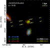 |
Fig. 1. False-colour RGB image of the galaxy GS-z9-0. The location of the NIRSpec slitlets (first nod) from the 1210 and the 3215 MSA mask designs are overplotted. Only one of the three (for 1210) and five (for 3215) ∼0.1″ dithered pointings are shown. |
In virtue of its allocation over multiple programmes, GS-z9-0 has collected a total exposure time with NIRSpec/MSA of 72.3 hours in PRISM/CLEAR, 44.3 hours in G395M/F290LP, and 16.3 hours in G140M/F070LP, as a result of combining 72 + 114, 18 + 96, and 18 + 24 individual integrations from both 1210 and 3215 programmes (19 groups/int, 2 integrations of 1400 s each per exposure, with a three-nodding pattern repeated over three-dithered and five-dithered pointings in 1210 and 3215, respectively). We note that the last visit (visit 5) of PID 3215 was affected by short circuits, reducing the exposure time compared to the original allocated time by 8400 s for PRISM and G140M observations (i.e. 6 integrations lost out of the requested 120), and by 33 600 s for G395M (24 integrations lost, equivalent to the full visit). The total exposure time in G235M/F170LP is instead 7 hours, resulting from solely the 1210 programme as such grating–filter combination was not repeated in 3215. In this paper, we leverage primarily the ultra-deep combined 1210 + 3215 data for PRISM, G140M, and G395M configurations, noting also that the C III] λ1909 emission line covered by G235M falls unfortunately in the gap between the two NIRSpec detectors. A summary of the observing modes and total exposure times is provided in Table 1.
NIRSpec observations of JADES-GS-z9-0.
The data reduction of the 3215 data follows the same recipe of 1210, as described in other papers of the JADES collaboration (e.g. Bunker et al. 2024; D’Eugenio et al. 2025). In brief, we adopt a three-nodding scheme for background subtraction, apply path-loss corrections appropriate for point sources (taking into account the intra-shutter position of the source in each nod and dither configuration), and reconstruct 2D spectra for each individual integration adopting a uniform wavelength sampling for the gratings (with a wavelength bin equal to the average native pixel sampling of the detector), while a highly non-uniform wavelength grid in the case of the PRISM, with the bin width set to account for the largely varying spectral resolution and to avoid oversampling of the line spread function.
From each 2D spectrum we then extract a 1D spectrum using a full-shutter window as driven by the light profile inferred from the brightest emission lines (to ensure minimal flux losses and avoid possible biases in the measured line ratios). We note that we also repeated the analysis adopting a narrower three-pixel boxcar extraction aimed at possibly maximising the signal-to-noise ratio, noting however a clear flux loss in the rest-optical lines as well as in the UV continuum shortwards of 2 μm in the PRISM spectrum, as well as no considerable improvement in the significance of the detection of the faintest lines, with the only notable exception of the N IV] λ1483 emission line in the G140M spectrum (see Sect. 2.2.1).
In order to obtain the final, combined 1D spectrum, in this work we have co-added the individual reduced 1D sub-spectra from both 1210 and 3215 for PRISM, G140M, and G395M by inverse-variance-weighted averaging over the surviving entries in each wavelength bin following five passes of iterative three-sigma-clipping aimed at flagging anomalous noise spikes representing outliers to the statistical noise in the data. This approach also allows us to obtain a more robust characterisation of the sources of noise present in the data by leveraging the large number of individual (while nominally identical) exposures in each grating/filter configuration (as discussed in the following section; see also Hainline et al. 2024b; Witstok et al. 2025a). Two-dimensional spectra are also reconstructed by the NIRSpec/GTO pipeline, but are generally not considered for extracting the 1D spectrum to avoid spurious effects and uncertainties possibly introduced by the heavy resampling of the data required to combine the 2D spectra of sources observed in different intra-shutter positions across different visits (and, in this case, also within multiple programmes).
The final, combined 1D and 2D PRISM spectra for GS-z9-0 are displayed in Fig. 2.
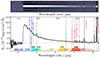 |
Fig. 2. PRISM spectrum of GS-z9-0 at z = 9.4327. The 2D (top) and 1D (bottom) spectra were obtained combining observations from the JADES 1210 and 3215 programmes. The pipeline error spectrum is reported in magenta. The main emission line features detected in the spectrum are marked in different colours, depending on whether they are also covered by G140M/F070LP (blue), G395M/F290LP (red), or observable only in the PRISM data (green). The FORECEPHO photometry extracted from available NIRCam wide- and medium-band imaging is also reported, showing good consistency in the flux calibration with the pathlosses corrected spectrum. |
2.2. Emission line fitting
We performed emission line fitting separately for low-resolution PRISM and medium-resolution gratings spectra. Formally, the error on each parameter of the fit was evaluated exploiting the output pipeline error spectrum. However, we also performed additional tests to assess the robustness of low-significance detections in both gratings and PRISM spectra by leveraging the large number of individual integrations in G140M (42) G395M (114), and PRISM (186) provided by the combined 1210 and 3215 datasets. More specifically, we generated 300 bootstrapped spectra by randomly sampling (with replacement) over the set of individual sub-spectra, after five passes of iterative 3σ-clipping have removed strong outliers at each wavelength bin. We then repeated the fitting process on each individual bootstrapped combined (averaged) spectrum, and took the square root of the variance of the resulting distribution as the error on the parameter. Such empirical bootstrapped uncertainties are expected to be more conservative than those estimated by assuming the output error spectrum from the pipeline, in that they implicitly take into account all possible sources of noise, including the correlated error among wavelength bins present in resampled NIRSpec spectra, which might not be fully accounted for by the pipeline (see also Maseda et al. 2023; Hainline et al. 2024b). We report the extracted emission line fluxes and equivalent widths for both our PRISM and gratings fitting in Table 2, where the signal-to-noise-ratio (S/N) quoted on the emission line fluxes is derived on the basis of both uncertainty estimates. Overall, we find bootstrapped-based S/N to be generally lower than those based on the pipeline error spectrum, and this is particularly true for medium-resolution grating spectra, whereas the pipeline error for the PRISM spectrum appears intrinsically more conservative in virtue of its attempt to rescale the noise to account for the correlation induced by the spectral resampling. A more detailed discussion about the noise model in NIRSpec spectra will be presented in a forthcoming paper (Jakobsen et al., in prep.). We also compared our results with those obtained via the joint continuum and emission lines modeling with PPXF (Cappellari 2017) as described in D’Eugenio et al. (2025), finding consistent results. Further details on the results of our fitting procedure are given below.
Emission line fluxes and rest-frame equivalent widths measured in PRISM and gratings (G140M and G395M) spectra.
2.2.1. Rest-frame UV spectrum
To begin with, we focus on the rest-frame UV region in the PRISM spectrum. We first performed a fit to the Calzetti et al. (2000) region down to 2600 Å (rest-frame), excluding the region bluewards of 1450 Å (rest-frame) to minimise the impact of the Lyα damping wing (we further discuss the modelling of the Lyα spectral break in Sect. 6). We modeled the underlying continuum with a power law, and included the following emission lines in the fitting procedure: N IV] λ1485 C IV λ1550, He II λ1640, O III] λ1666, N III] λ1750, C III] λ1909.
Each individual line was assumed as spectrally unresolved and modeled with a single Gaussian whose width was allowed to vary within ten per cent of the line spread function modeled from 1210 data by de Graaff et al. (2024), which takes into account the galaxy size and the relative NIRSpec intra-shutter position. Emission line doublets (e.g C III] λ1907,1909, N IV] λ1483,1486O III] λ1661,1666) or multiplets (e.g. N III] λλ1747–1754) were assumed unresolved in the PRISM spectra, whereas multiple components were included when fitting the gratings spectra. To model the N III] λλ1747–1754 multiplet in the PRISM, we set the line centroid to the average between the two brightest transitions in the multiplet (i.e. at 1751.83 Å). To aid the modeling of the line complex involving O III] λ1666 and He II λ1640 (which are partially blended at the PRISM resolution), their ratio was fixed to that measured from the G140M spectrum (see below). Furthermore, considering the proximity of the Si III] λλ1883,1892 doublet to C III] λ1909, and that such emission line has been observed in z∼2.5 galaxies (with relative intensity of ∼20−30% that of C III], e.g. Steidel et al. 2016), we included an additional Gaussian component1 to account for the Si III] doublet in our fitting procedure.
The results of fitting the rest-frame UV region of the PRISM spectrum are shown in the left-hand panel of Fig. 3: C IV λ1550, He II λ1640, O III] λ1666, and C III] λ1909 are detected above the continuum level at ≳5σ significance. From the same fit, we constrain the UV slope to βUV=−2.54±0.02. Although formally undetected (∼1.8σ significance), and despite its small contribution to the total flux of the complex, we note that including the Si III] λλ1883,1892 component (hatched green) provides a better match to the blue wing of the C III] line profile. Higher resolution observations of the C III] complex are needed to assess the real significance of the Si III] emission2, and we here note that none of the main results of the analysis depends on the inclusion (or not) of such component in the fitting procedure.
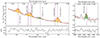 |
Fig. 3. Rest-frame UV emission lines in the PRISM spectrum of GS-z9-0. The best fit to the continuum and lines is shown in red. Detections at ≥4σ are marked in yellow, while marginal detections (∼3σ) are highlighted in green. The vertical purple lines mark the expected location of the emission lines based on the systemic redshift of the source. The bottom panels report the residuals of the fit and the 1σ uncertainty from the pipeline error spectrum. Left panel: Zoomed-in image of the region of the PRISM spectrum between 1.5 μm and 2.1 μm. In addition to clear detections of C IV, He II, O III], and C III], a marginal detection of N III] λ1750 is also highlighted. Right panel: Tentative detection of the very high-ionisation [Ne V] λ3426 emission line (ionisation potential 97.11 eV). The line is formally detected at ∼3σ from both the pipeline error spectrum and the bootstrapping approach described in Sect. 2.2. |
In addition, we report marginal detection (marked in green in Fig. 3) of the N III] λλ1747–1754 multiplet. The line is formally detected at 2.7σ assuming the error spectrum from the pipeline, whereas at 3σ adopting the bootstrapping approach. The N III] λλ1747–1754 emission arises in a region not contaminated by other emission lines, while the underlying continuum level is well constrained and anchored by the presence of adjacent high-EW emission lines (C III] and O III]); in other words, the best fit to the continuum is not affected by the inclusion (or not) of this specific line emission component. We discuss the implications of the possible detection of N III] λλ1747–1754 for the scenarios of chemical enrichment in GS-z9-0 (and, in particular, for the determination of the N/O abundance) in Sect. 5.
Conversely, N IV] emission is difficult to constrain in the PRISM fit. The fit improves if the N IV] component is not included, whereas forcing an additional Gaussian component at ∼1485 Å impacts the overall level of the continuum as well as the fit of the other emission lines in that region (especially of the adjacent C IV), decreasing the goodness-of-fit and highlighting the challenges in disentangling faint, low equivalent width line emission from the continuum at such low spectral resolution. When forcing the inclusion of the N IV] λ1483,86 component, we note that the line is formally detected at only ∼2σ, though the inferred flux is consistent with the low-significance N IV] λ1483 detection in the G140M spectrum (discussed below). We report the N IV] flux measured in the latter scenario in Table 2; nonetheless, we ultimately decided to exclude N IV] from our fiducial modeling of the PRISM spectrum (as shown in Fig. 3); this means that all the other line fluxes and the spectral slope were measured by fitting a model without such an additional Gaussian component.
Extending our fitting analysis to longer wavelengths, we also report the marginal detection of [Ne V] λ3426 (at ∼3.3σ with the pipeline error, 2.9σ with bootstrapping, right-hand panel of Fig. 3). To produce such very high-ionisation (97.11 eV) emission line requires an extremely hard photoionisation source. The presence of [Ne V] in galaxy spectra has been attributed to actively accreting black holes in AGN hosts, stellar continuum from an extremely hot ionising spectrum including Wolf–Rayet stars, or energetic radiative shocks from supernovae (Gilli et al. 2010; Izotov et al. 2012; Mignoli et al. 2013; Zeimann et al. 2015; Backhaus et al. 2022; Cleri et al. 2023) We discuss the implications of possible [Ne V] λ3426 detection in the determination of the dominant ionising source of GS-z9-0 in Sect. 3. However, we note that we do not detect any significant emission above the continuum level at the location of the [Ne IV] λ2424 emission line in the PRISM spectrum. One possible explanation for the absence of [Ne IV] λ2424 (in the presence of both [Ne III] and [Ne V]) is that, despite the lower ionisation energy of Ne3+ compared to Ne4+, the strength of the line is hampered on the one hand by its lower emissivity, while on the other by the relatively higher energy required to collisionally excite the ion.
Moving to the fit of the G140M spectrum, we report the detection of both O III] λ1666 and He II λ1640 at ∼7σ and ∼5σ significance based on the pipeline errors, respectively; based on the more conservative bootstrapping approach described above, both lines are instead detected at 3.5σ (right-hand panel of Fig. 4). During the fit, we fixed the velocity and width of He II λ1640 line to that of O III] λ1666, in order to restrict the fit only to the He II nebular component. However, we do not find any clear evidence for a residual broad component that could be associated with stellar winds features. The O III] λ1661 is not detected, however the ratio of O III] λ1666/O III] λ1661 is fixed by atomic physics to 2.93. The N III] λ1750 multiplet (whose components are almost fully resolved) is also undetected, and its 3σ upper limit is consistent with the expectations given the lower sensitivity of the G140M observations.
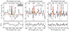 |
Fig. 4. Rest-frame UV emission lines in the G140M spectrum of GS-z9-0. In particular, we show a zoomed-in image of the region of the G140M spectrum around the N IV] doublet (left), C IV doublet (middle), He II, and O III] emission (right). The C IVλ1548, 51 doublet is resolved, but only the redder line is detected at >4σ significance. The C IV complex is blueshifted by ∼117 km s−1 compared to the systemic redshift, whereas no velocity offset is seen for O III] λ1666 and He II λ1640. The N IV] λ1483 line is tentatively detected at ∼3.4σ only in the 3 pixel extracted spectrum, whereas no significant N IV] λ1486 emission is found. |
When fitting C IV λλ1549,1551, we left the velocity and width of the two components of the doublet (spectrally resolved in G140M) free to vary, to account for possible resonant scattering through highly ionised gas that could impact the line profile (see e.g. Leitherer et al. 2011; Berg et al. 2019b; Senchyna et al. 2022; Topping et al. 2024). In general, the C IV λλ1549,1551 spectral feature is challenging to interpret due to its complex composite profiles, with possible contributions from narrow nebular emission, broad stellar emission, stellar photospheric absorption, and interstellar medium absorption and scatter. We detect (at 4.4σ assuming the pipeline error, at 3.2σ with bootstrapping) only one of the two C IV lines in the doublet, which we interpret as the ‘red’ C IVλ1551 component (middle panel of Fig. 3). If such interpretation is correct, the line appears shifted by ∼120 km s−1 with respect to the systemic redshift of the galaxy inferred from strong rest-frame optical lines, possibly indicative of resonant scattering through outflowing gas attenuating the blue component of the doublet, which has a relative oscillator strength ∼2 × higher than C IVλ1551. On the contrary, interpreting such emission line as C IVλ1548 would require a redshift >400 km s−1. Moreover, this would worsen the tension with the total flux and equivalent width of the total C IV doublet as inferred from the PRISM spectrum.
Finally, we report a tentative detection of N IV] λ1483, whose formal significance is however found to be >3 only in the narrower, 3 pixel boxcar extracted spectrum (left-hand panel of Fig. 4), whereas it is ∼2.8σ in the full-shutter extracted spectrum. Interestingly, no clear evidence of the redder line of the doublet (i.e. N IV] λ1486) is observed, which seems to exclude extremely high gas density in the system (see Sect. 4.1).
2.2.2. Rest-frame optical spectrum
We fit the rest-frame optical lines in both PRISM and G395M spectra modelling the underlying local continuum with a power law. Emission lines were assumed as unresolved and modeled with individual Gaussians, the only exception being the [O II] λλ3726,3729 doublet which is marginally resolved and modeled with two components when fitting the G395M spectrum. As shown in Fig. 5, rest-frame optical lines are well detected, with high signal-to-noise ratio, as already reported in Bunker et al. (2024), among others, based on observations from programme PID 1210. This includes not only a robust detection of the [O III] λ4363 auroral line, of specific interest for deriving chemical abundances (Sect. 4; see also Laseter et al. 2024), but also (more marginal) detections of high-order Balmer lines such as H9λ3835 and H10λ3797, which, in addition to well detected Hβ, Hγ, and Hδ, provide information to constrain the amount of nebular attenuation over a wide wavelength range (Sect. 2.3).
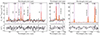 |
Fig. 5. Rest-frame optical emission lines in the G395M medium-resolution spectrum of GS-z9-0. The best fit to continuum and emission lines is overlaid in red; detected lines are highlighted (in green marginal ∼3σ detections). The left-hand panel shows a zoomed-in image of the region between [O II] λλ3726,3729 and Hδ, highlighting the detection of both strong lines and fainter Balmer lines such as H9 and H10. The middle panel shows the region around Hγ and the [O III] λ4363 auroral line, while the right-hand panel highlights the high S/N detections of the [O III] λ4959,5007 and Hβ complex. |
We derive a fiducial redshift for GS-z9-0 from the combined 1210 + 3215 spectrum by averaging over the brightest, isolated rest-frame optical lines, finding zG395M = 9.432681±0.000069 and zprism = 9.43774±0.00020 (mean and error on the mean), respectively. These values are consistent with those determined individually from 1210 and 3215 spectra, while revealing a significant discrepancy between G395M and PRISM, possibly caused by offsets in the wavelength calibration introduced by a non proper correction of the relative intra-shutter position in the determination of the wavelength solution (D’Eugenio et al. 2025).
We also note that existing flux calibration offsets between PRISM and grating spectra, as well as offsets as a function of wavelength and of the location on the MSA detectors, have been reported from the analysis of large galaxy samples observed with NIRSpec (e.g. Bunker et al. 2024; D’Eugenio et al. 2025). We tested this for GS-z9-0 by comparing the inferred flux for rest-optical lines redwards of [Ne III] λ3869 (to avoid further uncertainties on the continuum modeling in the PRISM spectrum introduced by the presence of a ‘Balmer jump’), and find that the gratings’ fluxes are higher by ∼10–12% compared to those measured from the PRISM, a value slightly larger than the average reported in JADES data release papers (Bunker et al. 2024; D’Eugenio et al. 2025). Therefore, to avoid introducing systematics associated with uncertain scaling factors, throughout this paper we consider only line ratios computed within the same spectral configuration (i.e. we do not use gratings-to-prism line ratios), and avoid adopting UV-to-optical line ratios to infer the physical properties of interest, where possible. As a general criterion, we primarily adopted line ratios from medium-resolution grating spectra where available, especially in the rest-frame optical (while testing the consistency of our results by comparing them with those inferred from PRISM-based fitting), whereas we resorted to line ratios measured from the PRISM when no detections were available from the gratings (as in the case of some rest-UV emission lines). In general, we note that, despite the offset in the absolute flux calibration between PRISM and gratings, we find that line ratios among the same set of lines derived from either configuration generally agree within their respective uncertainties.
2.3. Photometry and full spectral fitting
We performed FORCEPHO (Johnson et al. in prep.) fitting of the GS-z9-0 system to forward-model the light distribution and extract the photometry and morphological parameters from all the available NIRCam images in individual medium- and wide-band filters, namely F090W, F115W, F150W, F182M, F200W, F210M, F277W, F335M, F356W, F410M, F444W. The FORCEPHO setup follows that adopted in Tacchella et al. (2023b) and Baker et al. (2025), and we modeled the galaxy with a single Sérsic component. The extracted FORCEPHO photometry is reported in Table 3. Based on the morphological parameters derived from the FORCEPHO fitting, we infer a high compactness for this source, with an effective radius as small as Re = 110±9 pc.
FORCEPHO photometry from available NIRCam images in wide-band and medium-band filters.
We then modeled the full SED of the galaxy by simultaneously fitting PRISM spectrum and photometry with different codes, namely BEAGLE (Chevallard & Charlot 2016) and BAGPIPES (Carnall et al. 2018). We note that, given the excellent agreement between the pathlosses corrected PRISM spectrum and the extracted FORCEPHO photometry (see Fig. 2), no significant re-scaling of the spectrum is required in the procedure. We summarise the results of SED fitting from both codes in Table 4 and Fig. 6. The resulting best-fit spectra (corresponding to the minimum chi-square model) are shown in the top panels of Fig. 6, whereas in the bottom panels we report the posterior PDFs for stellar mass, stellar age, ionisation parameter, and metallicity (median, 16th, and 84th per centiles are marked with dashed black lines).
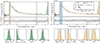 |
Fig. 6. SED fitting to the PRISM spectrum of GS-z9-0. The left-hand panel shows the fit performed with BEAGLE, while the right-hand panel shows the fit adopting BAGPIPES with a non-parametric star formation history. In both cases the upper panel shows the best-fit (minimum chi-square) model spectrum superimposed on the observed spectrum (in grey) and the FORCEPHO photometry (red points). The shaded areas mark the wavelength intervals masked during the fit (in particular the region around the Lyα break). The inferred non-parametric star formation history is depicted in the inset for the BAGPIPES fit. The lower panels report (from left to right) the marginalised posterior PDFs from the two fits for stellar mass, stellar age, ionisation parameter, and metallicity (relative to solar). |
Derived physical properties for GS-z9-0.
The BEAGLE setup mimics that employed in previous studies (e.g. D’Eugenio et al. 2024; Hainline et al. 2024b): in brief, we set an upper-mass cut-off for a Chabrier (2003) IMF to 300 M⊙, and modeled the SFH as a delayed-exponential with a burst occurring in the last 10 Myr. The metallicity of stars was tied to that of the nebular gas, and we implemented dust attenuation following the prescriptions of Charlot & Fall (2000). Overall, the best-fit spectrum provides a good match to the observed continuum and spectral shape, while struggling to match the intensity of some of the rest-frame UV emission lines such as He II and C IV. We discuss further on the possible mechanisms powering nebular emission lines in Sect. 3. The BEAGLE fit favours a recent history of star formation for GS-z9-0, (log(sSFR/yr−1) =−7.52, with an inferred light-weighted age of ∼3 Myr and an age of the oldest stars ∼12 Myr), a scenario consistent with the chemical abundance patterns discussed in Sect. 5. We infer a low metallicity (0.046±0.002 Z⊙), in good agreement with that derived from the Te-method (Sect. 4), and a relatively high ionisation parameter, log(U)  . For comparison, adopting for instance the photoionisation models presented in Berg et al. (2019b) we would derive a relatively lower log(U) =−1.78±0.10 based on the [O III] λ5007/ [O II] λλ3726,3729 ratio and given the measured Te-metallicity.
We explored the impact of systematics associated with the adoption of different stellar population synthesis models and star formation histories on our inferred physical properties by fitting the data also with BAGPIPES. In this setup, we employed the Binary Population and Stellar Synthesis (BPASS) v2.2.1 (Stanway & Eldridge 2018) templates including the evolution of binary systems, an upper mass cut-off of 300 M⊙ for a Kroupa IMF, dust extinction modeled by a Calzetti et al. (2000) law, and IGM attenuation models from Inoue et al. (2014). Nebular emission (in form of lines and continuum) was included by processing the BPASS stellar templates through the CLOUDY photoionisation code (Ferland et al. 2017). We left the gas metallicity and ionisation parameter as free parameters in the fit, but informed our priors (especially for metallicity) by exploiting the information empirically derived from emission lines (see Sect. 4); in particular, we adopt uniform priors on log(Z/Z⊙) ∈ [0.01, 0.25] and log(U) ∈[−3, −1]. Finally, we assumed a so-called non-parametric SFH following the recipe of Leja et al. (2019), defining six age bins counted backwards from the epoch of observations (the first two spanning 0–3 and 3–10 Myr, respectively). The priors on Δlog(SFR) values among adjacent bins were modelled as a Student's-t distribution with scaling factor σ = 0.3 (‘continuity’ model). The top right inset panel of Fig. 6 shows the inferred SFH, reporting the SFR in each of the temporal bins considered, as a function of lookback time. The BAGPIPES fit confirms the very recent history of mass assembly for GS-z9-0, predicting the majority of star formation to have occurred within the last two bins3, with a total stellar mass of log( M⊙, and a mass-weighted age of
  Myr, while the star formation rate averaged over the past 10 Myr is SFR
  M⊙ yr−1, in agreement with the values inferred both by BEAGLE (
 M⊙ yr−1), and by applying the calibration for low-metallicity systems from Reddy et al. (2022), Shapley et al. (2023a) to the measured Hβ flux ( = 5.46±1.04 M⊙ yr−1). Assuming the latter as fiducial value, and given the compactness of the system (Re∼110 pc), this translates into a high star formation rate surface density of ΣSFR = 72±14 M⊙ yr−1 kpc−2, and into a stellar mass surface density of
  M⊙ pc−2. We note BAGPIPES prefers an even more extreme ionisation parameter log(U) =−1.06 compared to BEAGLE (log(U) =−1.46), whereas the derived metallicity is fully consistent. A possible source of the discrepancy between the two inferred estimates of log(U) stems from its definition: in BEAGLE, the ionisation parameter is defined at the Strömgren radius (Eq. (7) in Gutkin et al. 2016), whereas BAGPIPES follows the prescription of Byler et al. (2017) and defines log(U) at the inner radius of the illuminated cloud, hence its value is expected to be systematically higher. Both SED fitting codes infer very low dust attenuation (AV
  and AV
  from BEAGLE and BAGPIPES, respectively), in agreement with the measured ‘decrement’among Balmer lines ratios discussed below.
Having access to spectrally resolved Hβ, Hγ, and Hδ in both G395M and PRISM observations (with additional detections of higher order H9 and H10 lines in G395M), we can obtain an independent constraint on the amount of nebular attenuation. In Fig. 7 we compare the observed Hγ/Hβ, Hδ/Hβ, H9/Hβ, and H10/Hβ ratios with the theoretical values expected for case B recombination, assuming a temperature of 20 000 K and density ne = 600 cm−3, consistent with the values measured directly from emission lines as detailed in Sect. 4. The ratios measured independently from G395M and PRISM spectra are in excellent agreement, and are consistent within their uncertainties with negligible-to-no dust attenuation. The best-fit AV derived from simultaneously fitting all the available Balmer line ratios with a Gordon et al. (2003) SMC attenuation curve and RV = 2.505 are AVG395M=−0.07±0.07 and AVPRISM = 0.01±0.07, respectively.
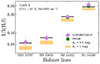 |
Fig. 7. Nebular attenuation inferred from Balmer decrements. The ratios of the different Balmer lines to Hβ, as measured from both G395M and PRISM spectra, are compared with the theoretical values set by Case B recombination (solid black bars) for Te = 20 000 K and ne = 600 cm−3 (consistent with electron temperature and density derived in Sect. 4). The ratios measured from both PRISM and gratings suggest negligible dust attenuation; the best-fit AV values are consistent with zero within 1σ uncertainty. |
Finally, by converting the UV luminosity density at 1500 Å rest-frame as measured in the PRISM spectrum, we derive a UV magnitude of MUV=−20.43, consistent with previous determinations based on the 1210 spectrum (Boyett et al. 2024). The inferred SFH, UV brightness, UV β slope, and negligible dust attenuation in GS-z9-0 aligns with observations of several other z>10 galaxies (e.g. Bunker et al. 2023; Arrabal Haro et al. 2023; Curtis-Lake et al. 2023; Castellano et al. 2024; Carniani et al. 2024), in agreement with theoretical scenarios invoking rapid star formation and dust-free environments (with dust possibly expelled by fast outflows, e.g. Ferrara 2024; Ferrara et al. 2025) as the responsible for the overabundance of luminous systems at high-z observed by the JWST (e.g. Ferrara et al. 2023; Mason et al. 2023).
3. Ionisation source
The ratios among different emission lines (either collisionally excited or produced by recombination) can be modeled to constrain the nature of the dominant source of photoionisation in galaxies. In the case of GS-z9-0, we leveraged the high S/N detections of several emission lines in both rest-frame optical and rest-frame UV regimes to explore a variety of different diagnostic diagrams. Rest-frame optical diagrams for this source (e.g. [O III]/ [O II] vs. ( [O III]+ [O II])/Hβ) have been explored already in Cameron et al. (2023a) as based on the data from the 1210 programme. In those diagrams, GS-z9-0 is observed to occupy the region belonging to local analogues of high-z galaxies characterised by low metallicity and a high ionisation parameter.
More recently, Scholtz et al. (2025) explored some rest-frame UV diagnostics with the aim of selecting robust type-2 AGN candidates within JADES. According to the criteria outlined in Scholtz et al. (2025), and following, in particular, a possible (∼4σ) detection of [Ne IV] λ2424 in the G235M spectrum (a high-ionisation emission line which requires very hard ionising continua to be powered, e.g. Brinchmann 2023), GS-z9-0 is classified as a type-2 AGN. As mentioned already in Sect. 2.2, this emission line, however, is formally undetected in our PRISM spectrum (we quote a 2.4σ significance based on the pipeline error spectrum, and only 1.6σ based on bootstrapping).
Here, we compare several UV-based diagnostics with predictions from suites of photoionisation models assuming different input ionising continua. These are presented in Fig. 8. More specifically, we focus our model predictions by exploring range of values in the physical properties matching (or in broad agreement with) those independently inferred for GS-z9-0 from the emission lines (e.g. for O/H, C/O). This is done in an attempt to limit the degeneracies induced by comparing model grids from different ionising sources under very different physical conditions, even when they do not match those (empirically and independently) estimated for an individual galaxy.
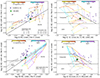 |
Fig. 8. Rest-frame UV diagnostic diagrams. The location of GS-z9-0 is reported and compared to a sample of local, high-z analogues from the CLASSY survey (Berg et al. 2022; Mingozzi et al. 2024). Top panels: C III] λλ1907,1909/He II λ1640 vs. O III] λ1666/He II λ1640 (C3He2-O3He2, left) and C III] λλ1907,1909/He II λ1640 vs. C IV λ1550/C III] λλ1907,1909 (C3He2-C43, right) line ratios are compared with photoionisation models by Gutkin et al. (2016) and Feltre et al. (2016) for constant star formation (solid lines) and NLR of AGNs (dashed lines), respectively. We fix the dust-to-metal ratio to ξd = 0.1, while varying metallicity and the ionisation parameter (colour-coded), C/O abundance, and slope α of the AGN continuum (different symbols). GS-z9-0 occupies a region fully consistent with star formation driven ionisation in the C3He2-O3He2 diagram, whereas it sits in a region of overlapping star formation and AGN grids in the C3He2-C43 diagram. In the C3He2-O3He2 diagram the solid and dot-dashed black lines represent the empirical demarcation between SF-, AGN-, and shock-driven ionisation as proposed by Mingozzi et al. (2024), whereas in the C3He2-C43 diagram we report the demarcation lines between SF, AGN, and composite proposed by Hirschmann et al. (2019). Bottom panels: Same as upper panels, but for single stellar population models from Plat et al. (2019, 3 Myr and 1 Myr old for solid and dashed lines, respectively, with fixed ξd = 0.3, and C/O = 0.1C/O⊙). The grids from 1 Myr stellar populations at low metallicity fully overlap those of AGN-like ionisation of higher metallicity and solar C/O (ξd = 0.1) in the C3He2-C43 diagram. |
More specifically, to model emission line ratios as predicted by ionisation from star formation, we adopted an updated version of the model grids described in Gutkin et al. (2016), Plat et al. (2019) for the two cases of constant star formation history (upper panels of Fig. 8) and single burst of different ages (lower panels of Fig. 8), respectively. We assumed an upper-mass cut-off of the IMF = 300 M⊙, a dust-to-metal mass ratio ξd = 0.1, and the gas density ne = 102 cm−3 as fiducial values. In the first scenario (constant star formation) we assumed a maximum stellar age of 100 Myr, whereas for the single stellar population scenario, we explored two bursts of 1 and 3 Myr age, respectively (more reflective of the SFH inferred in Sect. 2.3). We then explored a range of values in ionisation parameter (spanning between −3<log(U)<−1) and gas-phase metallicity (0.015<Z/Z⊙<0.7). In the upper panels, we explore also the variation in C/O abundance relative to solar ([C/O] ∈[−1, 0], where different [C/O] values are marked by different symbols), whereas in the middle panels [C/O] is fixed to −1 (in better agreement with that inferred from direct measurements as described in Sect. 4). To model line ratios produced by the narrow-line-region (NLR) of AGN instead, we adopted the models from Feltre et al. (2016), fixing ξd = 0.3 and ne = 103 cm−3 (more consistent with the typical densities of the NLR of AGN), while varying ionisation parameter, metallicity, and slope of the ionising continuum (α∈[−2, −1.2]). For AGN grids, the C/O abundance was fixed to the solar value.
In Fig. 8 we show the location of GS-z9-0 on two different diagrams based on rest-frame UV lines, namely C III] λλ1907,1909/He II λ1640 versus O III] λ1666/He II λ1640 (left-hand panel, hereafter C3He2-O3He2) and C III] λλ1907,1909/He II λ1640 versus C IV λ1550/C III] λλ1907,1909 (right-hand panel, hereafter C3He2-C43). These diagrams have been recently suggested as some of the most reliable in discriminating the dominant ionising source in galaxy spectra (Mingozzi et al. 2024), on the basis of observations of a sample of local, high-z analogues with full coverage of rest-UV spectrum from the CLASSY survey (Berg et al. 2022): these objects are included in our plots for comparison. In the C3He2-O3He2 diagram, GS-z9-0 occupies the region probed by low-C/O grids at low to intermediate metallicity from the star formation (SF) models, and appears inconsistent with the model tracks produced by AGN-NLR ionisation (while lying at the boundary of the SF-shocks demarcation line from Mingozzi et al. 2024). In the C3He2-C43 diagram instead, GS-z9-0 falls at the intersection between the SF and AGN model grids. Notably, 1 Myr SSP model grids (dot-dashed lines in the bottom panels) span a region of the diagram that overlaps with the AGN/NLR grids, making it harder to disentangle the dominant contribution to ionisation. However, we note that, because AGN grids are computed assuming a solar C/O abundance ratio, one could expect line-ratio grids for AGN-like ionisation of lower C/O (e.g. 0.1 × (C/O)⊙) to be shifted from those shown in the panel by a similar amount as observed between [C/O] =−1 and [C/O] = 0 SF-grids (at fixed other parameters): this in general would apply to all diagrams that intrinsically involve a dependence on the C/O abundance, and in the case of the C3He2-C43 diagram would make the agreement between GS-z9-0 and AGN-like grids worse.
However, the spectrum of GS-z9-0 reveals also the possible presence of a very high-ionisation emission line, which is challenging to explain by standard stellar population models, namely [Ne V] λ3426 (Fig. 3). Therefore, leveraging the detection of such emission line in the PRISM spectrum we explored different diagnostic diagrams: these are shown in the left and middle panels of Fig. 9 for C III] λ1909/He II λ1640 versus [Ne V] λ3426/C III] λ1909 (C3He2-Ne5C3) and [O III] λ5007/Hβ versus [Ne V] λ3426/ [Ne III] λ3869 (O3HB-Ne53), respectively. GS-z9-0 is located in-between SF and AGN grids in the C3He2-Ne5C3 diagram, but appears in slightly better agreement with AGN-ionisation (though still broadly consistent with SF models of very high ionisation parameter log(U) =−1), regardless of the dependence on C/O of the different grids (we recall that AGN/NLR models from Feltre et al. 2016 are computed assuming solar C/O). However, based on the O3HB-Ne53 diagram, GS-z9-0 appears totally consistent with AGN ionisation grids, with pure stellar population models struggling to produce significant [Ne V]. The advantage of the O3HB-Ne53 diagram is that it exploits the large difference in minimum energy required to produce [Ne V] and [Ne III] emission lines (which trace different ionisation zones Berg et al. 2021); moreover, it is based on lines closely spaced in wavelength (hence avoiding potential issues associated with wavelength-dependent slit loss correction and potential dust reddening), and it is also not affected by degeneracies in chemical abundances introduced by the use of emission lines of different elements. Such diagram has also been recently proposed as a possible way to discriminate between the ionisation produced by AGN with accreting supermassive black holes (MBH≥106 M⊙), AGN with intermediate-mass black holes (IMBH, MBH≲105 M⊙), and extreme stellar populations or even Population III stars (Cleri et al. 2023). In the middle panel of Fig. 9, we report the empirical demarcation lines for SF, AGN, and IMBH/Pop III stars based on the set of photoionisation models presented in Cleri et al. (2023, dashed black lines). Interestingly, we note that although GS-z9-0 resides in the ‘composite’ region, its [O III] λ5007/Hβ ratio (which is not as high as in local AGN given the low metallicity of the system) places it not far from the region dominated by IMBH/Pop III models. We note that in Cleri et al. (2023), the latter models assume zero metallicity for the stellar population but a slightly pre-enriched gas-phase metallicity of Z = 0.05 Z⊙ (similar to what inferred for GS-z9-0 based on Te measurements; Sect. 4) from primordial supernovae or stellar mass-loss events.
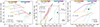 |
Fig. 9. Alternative diagnostic diagrams for GS-z9-0. The left and middle panels leverage the very high-ionisation (∼97 eV) [Ne V]λ3426 emission line, and the same set of models from Gutkin et al. (2016) and Feltre et al. (2016) as in Fig. 8. The diagram in the left panel (C3He2-Ne5C3) is sensitive to the C/O abundance, while the diagnostic considered in the middle panel (O3HB-Ne53) is not. Here, the location of GS-z9-0 is more in line with AGN-powered line ratios, especially in the [O III] λ5007/Hβ vs. [Ne V]/ [Ne III] diagram, where we show also the empirical demarcation lines between SF, AGN, and IMBH/PopIII models from Cleri et al. (2023). The right panel shows the C III] λ1909/He II λ1640 vs. N III] λ1750/O III] λ1666 diagram. The location of GS-z9-0 is compared with the set of photoionisation models for star formation (solid lines) and AGN/NLR (dashed lines) ionisation from Ji et al. (2024a). |
Finally, in the right-hand panel of Fig. 9, we plot a different diagnostic diagram, now leveraging the tentative detection of N III] λ1750 in the PRISM spectrum. In particular, we explore C III] λ1909/He II λ1640 versus N III] λ1750/O III] λ1666, which introduces explicitly the dependence on the N/O abundance. For this purpose, we employed a set of grids generated with CLOUDY, with 1 Myr old SSP templates from BPASS as the input spectra to model star formation, and a canonical SED with an effective big blue bump temperature of TBB = 106 K, a UV-to-X-ray slope of −1.4, a UV slope of −0.5, and an X-ray slope of −1.0 to model AGN continuum. We varied the metallicity Z/Z⊙ between 5×10⁻⁴ and 2, and the ionisation parameter log(U) between −3.5 and −1. We adopted the prescriptions from Groves et al. (2004) to compute the initial N/O (before dust depletion) at every given O/H, while C/O was scaled accordingly assuming solar abundance patterns. More details are given in Ji et al. (2024a). In this diagram, GS-z9-0 occupies a region consistent with stellar ionisation.
Summarising, on the basis of rest-UV diagnostics explored here, the line ratios observed in GS-z9-0 are consistent with ionisation from a population of massive and metal-poor stars, although the marginal [Ne V] λ3426 detection reported in the present work bring some evidence in support of the AGN scenario (see e.g. the recent observations of such transition in the galaxy GN42437 at z∼6, Chisholm et al. 2024). Nonetheless, radiative shocks driven by stellar winds and SN explosions have been also proposed as physical mechanisms capable of boosting the [Ne V] λ3426 emission in metal-poor star-forming galaxies (Izotov et al. 2012; Lecroq et al. 2024). In general, one should be probably careful about interpreting these diagnostic diagrams too rigidly. It is not unlikely that the nebular spectrum of GS-z9-0 is the result of mixing between different sources of ionisation, as recently suggested by the analysis of similar spectra of high-redshift galaxies (e.g. GS-9422 at z∼6, Tacchella et al. 2024, GN-z11 at z∼10.6, Bunker et al. 2023; Maiolino et al. 2024b, GHz2 at z∼12.3, Castellano et al. 2024), and decoupling their relative contribution would require more detailed modelling and a better understanding of the shape of the ionising continua of young, massive stellar populations.
4. Chemical abundances
The simultaneous detection of both nebular and auroral lines in the spectrum of GS-z9-0 enabled us to perform a detailed study of chemical abundance patterns in this galaxy, employing the ‘direct’, Te-method. Throughout this section we assume that ionisation comes primarily from star formation (see Sect. 3). However, we note that even in the case of possible AGN contribution to ionisation as discussed in Sect. 3, this does not prevent a direct measurement of the abundances via the auroral lines, provided that the proper ionisation correction factors (ICF) are included, which in the case of GS-z9-0 we expect to be similar between AGN and stellar spectrum with hard ionising continuum and/or high ionisation parameter.
Throughout this section, unless stated otherwise, we adopted PYNEB for chemical abundances derivation, with atomic data and collision strengths tabulated from the CHIANTI database. The errors on all the derived quantities were estimated by randomly perturbing the input emission line fluxes by their uncertainties (assumed Gaussian) and repeating the full procedure 100 times, taking the standard deviation of the distribution of values for each inferred parameter at each step of the procedure as our estimate of the (statistical) uncertainty associated with the fiducial value. Additional systematic uncertainties in the derivation of chemical abundances are discussed throughout individual sub-sections for each given element, and more broadly in Sect. 4.6.
4.1. Gas temperature and density
As a first step, we derive the temperature associated with the emitting region of O++ (hereafter t3) exploiting the high S/N detection of both [O III] λ4363 and [O III] λ5007 in the G395M grating spectrum. The gas density is simultaneously derived exploiting the [O II] doublet ratio, which is marginally resolved in G395M observations, while the temperature of the O+ emitting region (hereafter t2) was assumed in the process to follow the temperature-temperature relation from Izotov (2006) (i.e. t2 = 0.693t3+2810). We infer electron temperatures of t3 = 20137±1940 K and t2 = 16765±1345 K, respectively. The gas density is not well constrained (ne = 650±430 cm−3), given the [O II] λλ3726,3729 doublet is only marginally resolved in the G395M spectrum, however its best-fit value is consistent with typical densities measured in high-redshift galaxies (e.g. Isobe et al. 2023b). We assumed, therefore, ne = 650 cm−3 in our abundance calculations, noting that varying density between 100 and 1000 cm−3 would produce a difference in the inferred oxygen abundance of only ≈0.01 dex. Nonetheless, the tentative detection of N IV] λ1483 in the absence of N IV] λ1486 (Fig. 4) provides complementary information on the density of the emitting gas. This UV transition is another density-sensitive doublet which, in contrast to low-ionisation optical lines such as [O II] λλ3726,3729, traces much higher density regimes. The 3σ lower limit that can be placed on the N IV] λ1483/1486 ratio rules out extremely high gas densities (ne>104 cm−3), being in broad agreement with the density regime probed by the [O II] doublet. We can therefore reasonably exclude any significant contribution from high-density regions to the global emission line spectrum (whereas densities of the order of ne≈105−106 cm−3 have been measured in other bright UV galaxies at high-z, e.g. Topping et al. 2025), which might hamper the simultaneous interpretation of rest-UV and rest-optical features and possibly bias also the metallicity determined with the Te-method due to their unknown impact on emission lines of very different critical densities (Méndez-Delgado et al. 2023a; Marconi et al. 2024).
 |
Fig. 10. Electron density diagnostics. The [O II] λ3729/3727 ratio and the lower limit on the N IV] λ1483/1486 ratio, as well as the inferred electron densities, are reported as measured for GS-z9-0. The expected behaviour of the two line ratios as a function of density are depicted by the solid lines for Te = 2·104 K (with shaded regions spanning Te = 1−3·104 K). The lower limit on N IV] λ1483/1486 suggests no significant contribution from very high-density regions (ne≳104 cm−3), in broad agreement with the value inferred from the optical [O II] λ3729/3727 diagnostics. |
4.2. Derivation of oxygen abundance
We can then derive the relative ionic abundance of two elements comparing the intensity I(λ) in the emission lines of each species, while taking into account the different temperature- and density-dependent volumetric emissivity of the transitions J:
We computed the abundance of O++/H and O+/H from the [O III] λ5007/Hβ (assuming t= t3) and [O II] λλ3726,3729/Hβ (assuming t= t2) ratios, respectively, and derive log(O++/H) =−4.62±0.09 and log(O+/H) =−6.00±0.14.
One question is whether a significant fraction of oxygen could be in the triple-ionised state as possibly suggested by the detection of He II λ1640, since He2+ shares the same ionisation potential as O3+ (54.9 eV). We do not detect any significant O IV λλ1402,1404 emission in the G140M spectrum, and photoionisation modelling from Berg et al. (2019b) suggests a fractional contribution of O3+/O <0.01 given the measured ionisation parameter and the relative C3+/C++ ratio (see below). The measured 3-σ upper limit on the O IV λλ1402,1404 flux <1.82×10⁻¹⁹ erg s−1 cm−2 only provides an upper limit on O3+/O++ ≲0.4. We note that a small peak, possibly associated with O IV λλ1402,1404, is seen in the PRISM spectrum at ≈1400 Å, but the low spectral resolution makes it impossible to properly disentangle the O IV contribution from other nearby features such as [ Si][i v]λ1394, considering also the uncertainty on the intrinsic shape of the underlying continuum and the presence of the damping wing of the nearby Lyα break.
Alternatively, we can exploit an ICF for oxygen based on the relative abundance of single- and double-ionised Helium, following Torres-Peimbert & Peimbert (1977) and leveraging the similar ionisation potential of He++ and O3+ (see also Izotov et al. 2006; Valerdi et al. 2021; Dors et al. 2020, 2022). First, we estimated the intensity of He Iλ3889 emission by correcting the flux measured in the G395M spectrum by the contribution of the blended H8 Balmer line, which we infer from the expected theoretical ratio to the nearby Hδ (i.e. H8/Hδ = 0.406) assuming t2 and density as measured above, and under the assumption of no dust attenuation as suggested by the analysis in Sect. 2.3 (see also Fig. 7). Then, we computed the relative He+/H+ and He++/H+ abundances from the He Iλ3889/Hβ and He II λ1640/Hβ flux ratios, assuming t2 and t3 respectively. The ICF(O) is finally given by the (He+ + He++)/He+ ratio, which we measure as ICF(O) = 1.23, corresponding to a fractional contribution of O3+/O ∼19%. We note here that such an ICF is prone to large uncertainties due to the significant impact of radiative transfer effects on the He Iλ3889 line; while adopting the simplest optically thin case as fiducial, we explore variations in the assumed optical depth between τ∈[0, 5] implementing the correction coefficients from Benjamin et al. (1999), and estimate an uncertainty on the ICF(O) of ∼10%. To account for additional sources of uncertainties (e.g. He Iλ3889-H8 deblending, underlying line absorption) we conservatively include an additional 10% error budget on the ICF(O). The total oxygen abundance is hence O/H = ICF(O) × (O++/H + O+/H), and for GS-z9-0 this corresponds to 12 + log(O/H) = 7.49 ± 0.11, which we assume as our fiducial value in the following analysis. The fraction of doubly ionised oxygen over the total is O++/O = 0.84 ± 0.01. Neglecting instead any O3+ contribution (i.e. assuming O/H = O++/H + O+/H) would turn into 12 + log(O/H) = 7.40 ± 0.09. Finally, we note that repeating the procedure assuming emission line fluxes measured from the PRISM spectrum delivers a total (ICF-corrected) 12 + log(O/H) = 7.41 ± 0.13, lower but consistent with our fiducial value based on G395M within statistical uncertainties.
4.3. C/O abundance
We derived the C++/O++ abundance from the C III] λ1909/O III] λ1666 ratio, assuming the same electron temperature t3 when calculating the emissivity of the two ions. Because C III] λ1909 is observed only in the PRISM spectrum (while falling in the detector gap in G235M observations), here we adopt the C III] λ1909/O III] λ1666 ratio as derived from the PRISM, to avoid introducing uncertainties associated with flux calibration differences between PRISM and grating spectra. We also note that the relative temperature associated with C III] and O III] emission might be different, as C III] is possibly associated with an ‘intermediate-ionisation zone’, which could translate into a higher (lower) C++/O++ abundance by 0.15 dex (Garnett 1992; Croxall et al. 2016; Rogers et al. 2021; Jones et al. 2023) in case of lower (higher) C++ temperature, respectively. In principle, it would be possible to derive C++/O++ also from the C III] λ1909/ [O III] λ5007 ratio, however, we prefer to adopt C III] λ1909/O III] λ1666 to minimise uncertainties on the reddening correction and the choice of the attenuation curve given the short involved wavelength separation, as well as for consistency with the vast majority of literature studies.
Since the ionisation potential of O2+ is higher than that of C++ (54.9 eV vs. 47.9 eV, respectively), systems subject to hard ionising spectra such as GS-z9-0 may have a significant amount of carbon in the C3+ state. Therefore, we corrected the inferred C++/O++ abundance applying an ICF. The C IV λ1550 emission is detected in both the PRISM spectrum (though possibly blended with other spectral features) and in the G140M grating spectrum (though at lower significance), therefore we can exploit the C IV/C III] ratio to estimate the C3+/C++ relative abundance and derive the ICF for C/O or, alternatively, we can compare its strength to that of O III] to directly measure a C3+/O++ abundance; the two approaches give consistent results. We note that we have assumed that the C IVemission is purely nebular in origin (as suggested by its narrow line profile in G140M), although the full spectral profile of the C IV λ1550 doublet could be further complicated by resonant scattering through highly ionised gas, as well as interstellar absorption or contribution from stellar emission, that can either under- or overestimate the total C IV flux (Berg et al. 2018, 2019b; Senchyna et al. 2022). Given the likely non-negligible contribution of O3+ to the total oxygen abundance, we cannot simply assume that C/O = C3+/O++ + C++/O++. Therefore, we first computed C++/H+ and C3+/H+ by multiplying C++/O++ and C3+/O++ by O++/H+ as derived in Sect. 4.2, and then we assumed that the contribution from single-ionised carbon is negligible, so that the total C/H abundance is =C++/H+ + C3+/H+. Finally, we divided C/H by O/H to infer a total log(C/O) =−0.90 ± 0.12 dex. We note that if we assign the flux of the emission line detected in G140M to the red component of the C IV doublet (i.e. C IVλ1551), we can compare its strength to that of O III] λ1666 to obtain a grating-based measurement of the C3+/O++ abundance. This ultimately translates into a total log(C/O) abundance of −0.91±0.13, fully consistent with the previous estimate.
These values are also consistent, within their uncertainties, with the C/O inferred by assuming an ICF based on the photoionisation models presented by Berg et al. (2019b), assuming photoionisation from star formation and the ionisation parameter self-consistently inferred for GS-z9-0 from the same models (log(U) =−1.78), in which case ICF(C++/O++) = 1.20±0.054 and C/O = ICF × C++/O++, providing log(C/O) =−0.86±0.11. Finally, we estimated the C/O abundance via the equations outlined in Pérez-Montero & Amorín (2017), which deliver log(C/O) =−0.80±0.12.
Throughout the rest of the paper we assume the C/O derived including both C III] λλ1907,1909 and C IV λ1550 line fluxes as our fiducial estimate (i.e. log(C/O) =−0.90±0.11; statistical uncertainty), corresponding to ∼23% the solar C/O abundance, or [C/O] =−0.64. However, we note that C/O estimates based on the C III] λλ1907,1909/O III] λ1666 ratio and ICFs from photoionisation models generally provide C/O abundances up to ∼0.1 dex higher; therefore, we include an additional 0.1 dex uncertainty (co-added in quadrature) on the upper value to take into account these systematics.
4.4. N/O abundance
We estimated the N/O ratio by exploiting the detection of N III] λ1750 in emission. Leveraging the fact that the ionisation potentials of N++ and C++ are basically identical (47.448 eV and 47.887 eV, respectively), we assumed the C++/N++ abundance calculated from the C III] λ1909/N III] λ1750 ratio (accounting for the emissivity of all five lines of the N III] λ1750 multiplet) as a proxy of the relative C/N enrichment, finding log(C/N) = 0.03±0.19. Then, we combined this ratio with our fiducial C/O ratio, measured as described in the Sect. 4.3, to derive a total N/O of log(N/O) =−0.93±0.24.
Alternatively, we can exploit the tentative detection of N IV] λ1483 in the 3 pixel extracted G140M spectrum for an alternative derivation of N/O. From the N IV] λ1483/O III] λ1666 ratio5 we derived the N3+/O++ abundance (assuming t=t3), which we then multiply by O++/H to infer N3+/H; the same procedure is applied to N++/O++ (as measured from the N III] λ1750 in the prism spectrum) to infer N++/H, which we then co-added with N3+/H to derive the total N/H abundance (assuming negligible contribution from the singly ionised N+ state). Finally, we divided N/H by O/H to obtain a total N/O of log(N/O) =−0.77±0.18, higher than though consistent with our fiducial estimate.
Finally, based on the 3σ upper limit on the total flux of the N III] λλ1747–1754 multiplet from the G140M spectrum, we obtain a lower limit on log(C/N) >−0.24, and an upper limit on log(N/O) <−0.66.
4.5. Ne/O abundance
In the spectrum of GS-z9-0 we observe intense emission from Ne in its Ne++ form and the [Ne III] λ3869 emission line. We derived the Ne++/O++ abundance ratio assuming the t3 temperature for both ions, and corrected to the total Ne/O abundance exploiting the ICF presented in Amayo et al. (2021). We note that, given the different ionisation potentials of Ne+ and O+, coupled with the charge-transfer recombination rate of the two ions, the ICF is quite uncertain in low-ionisation, high-metallicity systems. However, in the case of GS-z9-0, the fractional contribution of unseen ionisation states to the total Ne/O is expected to be small, with ICF(Ne++/O++) = 1.02, nonetheless we conservatively assume a 10% uncertainty on the ICF. We therefore infer a total log(Ne/O) =−0.68 ± 0.06. We note that this value already includes the possible contribution from Ne4+: accounting separately for the marginal detection of [Ne V] λ3426 (but without applying any ICF) would deliver log(Ne/O) =−0.73 ± 0.07.
4.6. Systematics in the abundance measurements
Despite the high S/N of most of the emission lines detected in the GS-z9-0 spectrum, a number of additional systematics uncertainties affect our chemical abundance measurements beyond those already mentioned in the previous sections. Some of the most relevant are associated with electron temperatures, as briefly discussed here.
In Sect. 4 we have adopted the temperature inferred from the [O III] 4363/ [O III] λ5007 ratio as our fiducial estimate for t3. However, the O III] λ1666/ [O III] λ5007 is another temperature diagnostics that can be adopted in studies of high-z galaxies where the [O III] 4363 emission line is not detected (e.g. Revalski et al. 2024). Exploiting the O III] λ1666 flux measured from G140M (where it is spectrally resolved from He II λ1640), we infer t3 = 24 405 ± 1490 K, higher (significant at 1.6σ) than that inferred from [O III] λ4363. This propagates into a lower inferred O/H by 0.15 dex, whereas only in a difference of 0.05 dex in C/O, as the C III] λ1909/O III] λ1666 ratio is only mildly sensitive to temperature. We include further 0.1 dex systematic uncertainty on the lower value of log(O/H) to reflect this difference.
The origin of this discrepancy is uncertain. Although similar differences in t3 as inferred from either O III] λ1666 or [O III] 4363 have been reported before (e.g. Berg et al. 2016), these were generally attributed to offsets in the flux calibration between O III] λ1666 and [O III] λ5007 (which, before the advent of JWST, were usually observed by instruments on different facilities), or to the large uncertainty on the relative reddening correction between UV and optical wavelength regimes. In our case, assuming no attenuation correction as suggested by the measured Balmer decrements (see Sect. 3), this would imply an unrealistic (and never observed in NIRSpec to our knowledge) factor ×1.9 offset in the flux calibration between G140M and G395M (in the sense that O III] λ1666 is almost a factor of two brighter than it should be) in order to match the t3 estimates from optical and UV lines.
A more physically motivated explanation involves the fact that O III] λ1666 and [O III] λ4363 come from different energy levels, with different critical densities and different collisional excitation rates; hence, their ratio also depends on the gas density, and can therefore be impacted by the presence of density inhomogeneities within galaxies (e.g. Marconi et al. 2024). Moreover, when different temperature estimators rely on collisionally excited lines originating from well-spaced energy levels, the inferred temperatures can also differ by an amount that depends on the variance of the temperature distribution within the nebula, even if the diagnostics pertain to the same ionic species (O++ in this case). This possibly suggests that rest-frame UV and rest-optical emission lines (even of the same ionic species) could originate from different regions in the galaxy, and that this effect could be particularly relevant in high-redshift systems similar to GS-z9-0 characterised by highly ionised gas, where temperature inhomogeneities are expected to be enhanced. This effect has been historically described with the t2 parameter (see Peimbert & Costero 1969, and more recently Méndez-Delgado et al. 2023b), which represents the root mean square deviation from the average temperature. In the case of GS-z9-0, the difference measured between O III] λ1666-based and [O III] λ4363-based temperatures would translate into t2∼0.24, a value higher than measured in local HII regions. However, given such a large t2 one would expect a much lower temperature inferred from the nebular continuum (∼11 000 K) than observed. Fitting a broken power-law continuum to the Balmer jump region of GS-z9-0 one infers T = 2.0±0.5×10⁴ K, consistent with the Te-based measurements presented above (see also Ji et al. 2024b).
In a similar manner, another source of systematic uncertainty is associated with the adoption of the same temperature for the emitting region of [O III] λ5007 and C III] λ1909. As C++ has a lower ionisation energy than O++, it might be better associated with an ‘intermediate ionisation region’, probed by ions such as S++ (Berg et al. 2021). Since we do not have access to transitions suitable for directly inferring the temperature of such intermediate zone, we can employ Eq. (3) from Berg et al. (2020), which provides Tintermediate = 23 150 K and consequently a C++/O++ ratio lower by 0.20 dex (which propagates into a total C/O lower by 0.13 dex, if still assuming the same t3 for O++ and C3+). We note, however, that such temperature-temperature relation can be quite scattered and uncertain, especially at high temperatures and ionisation (Hägele et al. 2006; Binette et al. 2012; Berg et al. 2015; Jones et al. 2023); moreover it is mostly calibrated on samples of local HII regions. Therefore, we chose to not adopt it in our fiducial analysis, nonetheless we note that the amount of systematic uncertainty it carries can be significant.
A similar argument can also be made for the temperature-temperature relation employed to infer the abundance of singly ionised oxygen. In Sect. 4 we have adopted the t2–t3 relation from Izotov et al. (2006); adopting instead the relation calibrated by Pilyugin et al. (2009), among others, or the theoretical relation by Campbell et al. (1986), provides higher t2 by ∼2500 K and ∼322 K, respectively. However, this translates to a total Δlog(O/H) of ≲0.005 dex, since O+ is contributing only ∼2.5% to the total oxygen abundance.
Finally, to take into account the abundance of highly ionised ionic species such as C3+ and N3+, Berg et al. (2021) proposed a four-zone ionisation model to provide a more accurate description of the regions of line emission in galaxies characterised by ‘extreme’ conditions. In such framework, the temperature of the very high ionisation zone is better probed by the [Ne III]λ3342/λ3868 ratio than the classical t3 (as the ionisation potential of Ne2+ is higher than that of O2+). However, we do not detect [Ne III]λ3342 in our prism spectra, and therefore we had to assume t3 when computing the emissivity of C3+ and N3+ in our carbon and nitrogen abundance calculations. The extent of the associated systematic uncertainty is difficult to assess. Berg et al. (2021) find only a mild (mostly within 1-σ uncertainty) impact on the total inferred O/H, C/O, and N/O when adopting either the three- or four-zone ionisation model for the galaxies J104457 and J141851, though we note that the fraction of highly ionised species of oxygen, carbon, and nitrogen are minimal in those systems. On the other hand, we note that our derivation of the N/O abundance in GS-z9-0 follows from the measurement of C/N, which is based on emission line ratios with relative weak temperature dependence, whereas for what concerns the C/O derivation, conservatively assuming a temperature much higher than t3 (e.g. 25 000 K) as representative of the C IV emitting region (as it would be in case C3+ preferentially occupies a region closer to the ionising source) would translate into a lower total inferred C/O by ∼0.24 dex compared to our fiducial value. This effect might be even larger for higher states of neon such as Ne4+ that could originate from extremely high-ionisation regions (especially in the case of the NLR of AGN); however, given the small relative Ne4+/Ne++ abundance, we verified that even assuming a temperature as high as 25 000 K it would not significantly impact the final inferred Ne/O abundance (which would be lower by 0.02 dex compared to our fiducial estimate).
To account for the hereby discussed effects, we include an additional 0.15 dex of systematic uncertainty also on the C/O and N/O6 abundances beyond the formal statistical uncertainties propagated from the error on the measured line fluxes. This, together with the uncertainties on C/O from photionisation-based ICFs discussed already in Sect. 4.3, translates into the final uncertainties quoted in parenthesis in Table 4.
5. Possible scenarios for chemical enrichment
In Fig. 11 we report GS-z9-0 (green hexagon marker) on different diagrams which explore trends between various chemical abundance patterns (i.e. C/O, N/O, and Ne/O) and metallicity (probed by oxygen abundance). The solid errorbars report the formal statistical uncertainties on our fiducial estimates of chemical abundances, whereas dashed errorbars account for the systematics discussed in Sect. 4.6.
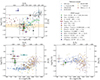 |
Fig. 11. Chemical abundance patterns in GS-z9-0. The location of GS-z9-0 is marked by the green hexagon; the solid errorbars report the formal statistical uncertainties on our fiducial values and the dashed errorbars account for additional systematic uncertainties, as discussed in Sect. 4.6. The dashed black lines in the diagrams mark the solar abundance values. We compare GS-z9-0 with a compilation of recent abundance measurements in high-z galaxies from JWST, i.e. from Ji et al. (2024a) (plain marker for optical-based abundances and hatched marker for UV-based abundances), Topping et al. (2024), Isobe et al. (2023a) and Jones et al. (2023) at z∼6, Topping et al. (2025) at z∼7, Arellano-Córdova et al. (2022) at z∼8.5, Napolitano et al. (2024) at z∼10, Castellano et al. (2024) at z∼12, as well as upper limits on GN-z11 and GS-z12 from Cameron et al. (2023b) and D’Eugenio et al. (2024), respectively. We also include measurements in Milky Way disk and halo stars, local HII regions, local dwarf galaxies, z∼2 galaxies, and damped Lyman-alpha systems (DLA). Upper left panel: C/O vs. O/H diagram. The C/O abundance range predicted from type II SN yields from Tominaga et al. (2007) is marked by the golden hatched region, whereas the C/O vs. O/H pattern from Kobayashi et al. (2020) galactic chemical evolution (GCE) models is shown by the green sequence. The C/O level observed in GS-z9-0 is consistent with the enrichment expected from core-collapse SNe for a recently assembled, low-metallicity system. Bottom left panel: N/O vs. O/H diagram, reporting for GS-z9-0 both the N/O as inferred from the detection of N III] λ1750 in the PRISM spectrum and the C/N ratio (fiducial value, plain green hexagon), as well as that based on the marginal detection of N IV] λ1483 in the G140M spectrum (hatched symbol; see Sect. 4.4). The N/O measured in GS-z9-0 is higher than the plateau occupied by local galaxies and HII regions at low metallicity, although the nitrogen enhancement observed in this galaxy appears less extreme compared to other high-z systems recently observed by JWST. Bottom right panel: Ne/O abundance for GS-z9-0, which we observe to be consistent with the abundance pattern expected at low metallicity for α-elements. Additional references for literature points: compilation of MW stars (Gustafsson et al. 1999; Akerman et al. 2004; Fabbian et al. 2009; Nissen et al. 2014); compilation of z ∼0 galaxies and HII regions (Tsamis et al. 2003; Esteban et al. 2004, 2009, 2014, 2017; García-Rojas et al. 2004, 2005, 2007; Peimbert et al. 2005; García-Rojas & Esteban 2007; López-Sánchez et al. 2007; Toribio San Cipriano et al. 2016, 2017; Senchyna et al. 2017); HII regions from CHAOS (Berg et al. 2016, 2019b); blue compact dwarfs (BCD) and giant HII regions (GHR) from BOND (Vale Asari et al. 2016); z ∼2 galaxies (Fosbury et al. 2003; Erb et al. 2010; Christensen et al. 2012; Bayliss et al. 2014; James et al. 2014; Stark et al. 2014; Steidel et al. 2016; Vanzella et al. 2016; Amorín et al. 2017; Berg et al. 2018; Mainali et al. 2020; Matthee et al. 2021; Rigby et al. 2021; Iani et al. 2023); DLAs at z∼3−4 (Cooke et al. 2017; Saccardi et al. 2023). |
The top left panel shows the C/O versus O/H diagram, with GS-z9-0 compared with previous abundance determinations in both local and high-redshift systems, as well as those measured in Milky Way (MW) disk and halo stars (see caption of Fig. 11 for details and references). The low C/O abundance in GS-z9-0 is comparable to that observed in metal-poor systems at lower redshift, being in line with some of the most recent determinations in z≳6 galaxies observed with JWST from Arellano-Córdova et al. (2022, z∼8.5), Jones et al. (2023, z∼6.23), Isobe et al. (2023a, z∼6.2), Topping et al. (2024, z∼6.3), Castellano et al. (2024, z∼12.3; whereas in contrast, the upper limits on GS-z12 from D’Eugenio et al. 2024 suggest significantly super-solar C/O in that system at z∼12.5).
Given the very young age of the system (mass-weighted age ∼30 Myr as inferred from the SED fitting), we expect chemical yields dominated by core-collapse SNe (CCSNe), whereas low- and intermediate-mass stars in their AGB phase (with lifetimes ≈100 Myr) would not have had enough time to significantly contribute to the overall enrichment of the galaxy. The datapoint for GS-z9-0 on the C/O versus O/H plane is consistent with the range in C/O predicted by integrating the yields of type II SNe from very metal-poor stars over a Salpeter IMF (Tominaga et al. 2007, golden shaded region). In the same panel, we also compare our observations with the C/O enrichment pattern predicted by galactic chemical evolution (GCE) model of the solar neighbourhood presented in Kobayashi et al. (2020, shaded green curve), which follows the time evolution of elemental abundances in a one-zone model with ISM instantaneously mixing but no instantaneous recycling approximation (i.e, the delay of chemical enrichment from different sources is taken into account), assuming a Kroupa (2008) IMF and solar abundances from Asplund et al. (2009). Our observations agree well with the sequence in C/O of Kobayashi et al. (2020) at the measured oxygen abundance for GS-z9-0, as this system resembles the C/O enrichment pattern of metal-poor stars in the MW.
The position of galaxies on the C/O versus O/H diagram is also sensitive to the amount of metals lost due to outflows. Possible indications of outflowing gas in GS-z9-0 comes from the observed blueshifted C IV λλ1549,1551 doublet in G140M (Fig. 3). The spread observed in C/O at fixed O/H in samples of metal-poor local dwarfs and z∼2 galaxies can be reproduced not only in terms of different SFH and IMF slopes, but even accounting for selective oxygen removal in outflows driven by CCSNe (Yin et al. 2011; Berg et al. 2019b) According to the formalism from Berg et al. (2019b), developed to model the C/O versus O/H pattern observed in local, metal-poor dwarf galaxies, the low O/H and low C/O measured in GS-z9-0 would indicate negligible oxygen-enhancement in SN-driven outflows. However, we note that in such a framework low C/O abundances are associated with single, long bursts of star formation characterised by relatively small star formation efficiency, whose timescales (∼300−400 Myr) can be hardly reconciled with the inferred age and star formation history of GS-z9-0.
In the bottom left panel of Fig. 11, we report instead the location of GS-z9-0 on the N/O versus O/H diagram. Based on the N/O derived from the N III] λ1750 detection in the PRISM spectrum as detailed in Sect. 4.4, GS-z9-0 appears nitrogen-enriched compared to the typical range of values observed in local, low-metallicity dwarf galaxies (e.g. Pérez-Montero & Contini 2009; Berg et al. 2012; Vale Asari et al. 2016; Vincenzo & Kobayashi 2018b) as predicted by primary nitrogen enrichment, showcasing instead N/O consistent with the solar value. An even (slightly) higher N/O is inferred when including the tentative N IV] λ1483 detection in the G140M spectrum (hatched green symbol in the panel).
A similar pattern characterised by high N/O abundance at low O/H and low C/O has been already observed in several high-redshift (z>6) galaxies observed with JWST (e.g. Cameron et al. 2023b; Isobe et al. 2023a; Topping et al. 2024, 2025; Napolitano et al. 2024; Castellano et al. 2024; Schaerer et al. 2024), although we note that GS-z9-0 does not reach the same level of N/O enhancement as the aforementioned systems, which are observed to be significantly super-solar in N/O. Low C/N ratios are also often observed in the so-called ‘nitrogen-loud quasars’ (Batra & Baldwin 2014), as possibly produced by the enrichment from AGB stars or SNe occurring within the small, local volume of the narrow-line or even broad-line region of AGN (Maiolino et al. 2024b). Such a scenario can produce a chemical stratification between central, denser regions and the rest of the galaxy, which is imprinted on the largely different N/O derived from UV lines (tracing dense, highly ionised regions) and optical lines (tracing the bulk of the galaxy) as observed for example in the z∼5.5 active system GS-3073 (Ji et al. 2024a, for which UV-based and optical-based measurements are marked by hatched and plain brown octagons in Fig. 11). However, in the case of GS-z9-0 the contribution from AGB stars is strongly disfavoured given the inferred age and SFH of the system, and moreover it would be difficult to reconcile with the simultaneous low O/H and C/O.
The N/O pattern seen in GS-z9-0 also resembles that of nitrogen-enhanced metal-poor (NEMP) stars observed in the Galactic halo (Belokurov & Kravtsov 2023), while even higher levels of N-enhancement (log(N/O) ≳0) are seen in some dwarf stars within globular clusters (Carretta et al. 2005; D’Orazi et al. 2010) as well produced by old stellar populations in metal-poor ultra-faint dwarf galaxies (UFDs), systems formed at high redshift which are now completely gas depleted (Alexander et al. 2023). It has been suggested that these objects share a similar chemical composition as some of the most extremely nitrogen-rich galaxies observed by JWST (e.g. Charbonnel et al. 2023; Senchyna et al. 2024; Marques-Chaves et al. 2024; Topping et al. 2024), which in turn could represent their high-z progenitors.
Despite GS-z9-0 showing a relatively lower N/O compared to such systems, its N-enrichment level compared to the N/O versus O/H plateau, coupled with the concentrated star formation, could still be consistent with proto-globular cluster formation contributing, to some extent, to the observed integrated galaxy spectra. Although the (mild) constraints on the density of the highly ionised gas in GS-z9-0 provided by UV-diagnostics (based on the low-significance detection of N IV] λ1483 in the absence of N IV] λ1486) seems to exclude the presence of extremely dense regions, the low S/N of the G140M spectrum, the C III] λ1909 doublet (an additional potential density diagnostics) unresolved in the PRISM spectrum, and the putative AGN contribution suggested by the presence of very high-ionisation emission lines prevents us from drawing more definitive conclusions in this sense.
Overall, in GS-z9-0 we therefore possibly observe signatures of chemical enrichment mechanisms beyond that of pure CCSNe, as depicted by the relatively high N/O and low C/N. Several scenarios have been explored to reproduce similar abundance patterns in high-z galaxies, including ejection of CNO-cycle processed material in stellar winds from Wolf-Rayet (WR), large mass-loss rates during the evolution of very massive stars (VMS) or even supermassive stars (SMS), and contribution from fast-rotating Population III stars (e.g. Nagele & Umeda 2023; Watanabe et al. 2024; Vink 2024; Marques-Chaves et al. 2024; Nandal et al. 2024). Here, we compare the observed C/O, N/O, and C/N abundances in GS-z9-0 with a set of GCE models from Kobayashi et al. (2020), Kobayashi & Taylor (2023), with updated carbon yields for WR stars. In particular, we assumed a single-burst model following similar prescriptions as in Kobayashi & Ferrara (2024), and explored the impact of different IMF shapes on the nucleosynthetic patterns of the most massive stars, and hence on the observed chemical abundances. In Fig. 12 we overplot the tracks from three different realisations of the model onto the C/O versus O/H, N/O versus O/H, and C/N versus O/H diagrams, respectively. In particular, the blue track represents the predictions assuming a standard Kroupa (2008) IMF (with high-mass end slope x = 1.3), whereas the magenta and red tracks assume a top-heavy IMF (x = 0) of Population III stars with upper mass limits of 120 M⊙ and 280 M⊙, respectively. Each model track reaches the observed value of O/H for GS-z9-0 after 4.05 Myr.
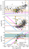 |
Fig. 12. Evolution of CNO abundance ratios as a function of oxygen abundance for single starburst models with different IMFs, based on the framework of galactic chemical evolution models from Kobayashi et al. (2020). The symbols are as in Fig. 11, with GS-z9-0 in green and other high-z objects observed by JWST from the literature highlighted in yellow. Shaded regions in the C/O vs. O/H and C/N vs. O/H panels mark the range allowed by pure CCSNe based on the yields from Tominaga et al. (2007) and Watanabe et al. (2024), respectively. The blue model assumes a standard IMF (with high-mass end slope x = 1.3), whereas the magenta and red curves assume a top-heavy IMF (with flat slope) for massive stars in the range 30–120 M⊙ and 100–280 M⊙, respectively, with the latter including PISNe. For each model, the curve reaches the observed O/H in GS-z9-0 after 4.05 Myr. The combined CNO pattern of GS-z9-0 is better matched by models with underlying top-heavy IMF. In order to reproduce the abundance patterns of GS-z9-0 with a standard IMF, a more tailored double-burst model (with two bursts separated by 100 Myr, dashed orange line) is needed, similar to that proposed by Kobayashi & Ferrara (2024) to explain the nitrogen enhancement in GN-z11. |
Evolutionary tracks with underlying top-heavy IMF provide the best match to the position of GS-z9-0 in all three diagrams simultaneously, with WR stars producing the required enrichment in N/O (magenta track). We note that the red track, which includes a contribution from pair-instability supernovae (PISNe) of massive PopIII progenitors (>150 M⊙), also provides a good match to the observed abundances, maintaining the C/O to a level more consistent with that observed in GS-z9-0, while slightly underpredicting (overpredicting) N/O (C/N). Additional abundance measurements of elements such as sulphur, argon, or iron would be required to better constrain the possible signatures of PISNe and discriminate their relative contribution.
In addition, we also explored a ‘dual burst model’ (dashed orange track in Fig. 12) that reproduces the abundances in GS-z9-0 without the need to invoke top-heavy IMFs, similarly to what has been developed by Kobayashi & Ferrara (2024) to match the abundance patterns observed in GN-z11. Contrary to single burst models, this model assumes a more tailored star formation history, which is halted for a period of ∼100 Myr between two strong bursts. Such a model produces a quick enhancement of both C/O and N/O via WR stars just after the second burst, which occur within a pre-enriched ISM from the first star formation episode. While N/O can be regulated (and lowered) by increasing the timescale of star formation for the second burst (making it less extreme), this model slightly overpredicts the C/N level compared to what observed in GS-z9-0.
Finally, we display the measured Ne/O versus the O/H abundances for GS-z9-0 in the bottom right panel of Fig. 11, where we compare our measurement at z∼9.4 with the values inferred for high-z galaxies ERO-4590 at z∼8.5 by Arellano-Córdova et al. (2022), GN-z9p4 at z∼9.4 (Schaerer et al. 2024), as well as with measurements in blue compact dwarfs and extragalactic giant HII regions from Vale Asari et al. (2016), and in HII regions of local galaxies from the CHAOS sample as studied in Berg et al. (2020). As neon is an α-element, its production mechanisms and timescales are expected to closely follow that of oxygen, with no significant trend in Ne/O as a function of metallicity. The Ne/O abundance measured in GS-z9-0 is fully in agreement with the low-metallicity tail in the diagram as probed by local blue compact dwarf galaxies. Although a possible evolution in the Ne/O abundance pattern at z>3 has been suggested on the basis of the observed scaling relation between stellar mass and the [Ne III]/ [O II] line ratio (Shapley et al. 2023b), and Isobe et al. (2023a) find that significantly lower Ne/O ratios in some z>6 galaxies can be explained by models of CCSN ejecta including massive (>30 M⊙) progenitors, here we find no evidence for a deviation in the Ne/O abundance in GS-z9-0 compared to the chemical abundance patterns of local, metal-poor compact galaxies.
6. Lyα emission and implications for reionisation
Despite the MSA detector gap cutting the G140M spectrum just bluewards of the systemic Lyα wavelength, it still covers the onset of the Gunn & Peterson (1965) absorption trough. Notably, an emission feature stands above the continuum just redwards of the systemic redshift Lyα at z = 9.4327. If we interpret this feature as Lyα emission, we can put more stringent constraints on the shape of the transmission curve, the escape fraction of Lyα photons, and the possible existence of an ionised bubble around the system. We fit this emission line with a single Gaussian component and modeled the underlying continuum with a broken linear component as shown in Fig. 13, measuring a flux of 2.18 × 10⁻¹⁹ erg s−1 cm2, significant at 2.7σ (2.3σ based on bootstrapping7). The emission line centroid is redshifted by 450±145 km/s with respect to the systemic redshift, the FWHM of the line is 380±130 km/s, and the estimated rest-frame EW of the line above the G140M continuum level is 31±16 Å.
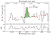 |
Fig. 13. Zoomed-in image of the tentative (∼2.7σ) detection of the Lyα emission line in the G140M spectrum of GS-z9-0. The emission feature is observed shifted by ∼450 km s−1 redwards of the systemic Lyα at redshift z = 9.4327. |
Based on the theoretical ratio between (unattenuated) Lyα and Hβ fluxes (Lyα/Hβ = 25.1 for case B recombination, T = 20 000 K, ne = 650 cm−3), and assuming the Hβ flux measured from the G395M spectrum, we derive an intrinsic Lyα flux of 1.89×10⁻¹⁷ erg s−1 cm2, from which we infer that the Lyα emission has been attenuated down to ∼1% of its intrinsic flux. Such a low Lyα escape fraction, coupled with the presence of emission observed only significantly redwards of the systemic wavelength, and the negligible dust attenuation, provides evidence against the presence of a large ionised region surrounding GS-z9-0. Such an ionised bubble would likely allow a higher fraction of Lyα photons to escape (given the intrinsic predicted flux) and, under the assumption of a broad, symmetric intrinsic Lyα profile, would have also caused the line profile to spill across to the blue of the systemic redshift.
In addition to the detection of Lyα emission, we leverage the robust redshift determination enabled by the bright emission lines detected in GS-z9-0 to remove the redshift-degeneracy in modeling the Lyα break as observed (at high signal-to-noise ratio) in the PRISM spectrum, and get more insights into the properties of the surrounding medium, the possible extent of any ionised region, and the presence (or absence) of large column densities of neutral gas along the line of sight. We modeled the attenuation due to neutral IGM along the line of sight following the prescriptions from Inoue et al. (2014), and included treatment of the full optical depth (including damping-wing absorption) of Lyα photons following Dijkstra (2014) and Mason & Gronke (2020, for further details, see Witstok et al. 2024), under the assumptions of the gas in the IGM having mean cosmic density and T = 1 K, while gas in the ionised bubble is fully ionised (residual neutral fraction xHI = 10−8) with T = 104 K. We applyed such transmission curve to a power-law spectrum modelling the continuum bluewards of 1500 Å rest-frame8, to avoid the region contaminated by emission lines, and we included the contribution from the Lyα emission matching flux, velocity and width as observed in the G140M spectrum a posteriori into the model (i.e. after attenuating the intrinsic spectrum), as it could possibly affect the observed profile9. We then convolved the attenuated model by the PRISM line spread function provided by de Graaff et al. (2024) and resampled it to the PRISM wavelength grid before comparing to the data. In order to properly account for the inter-correlation between adjacent wavelength bins in the fitting procedure, the χ2 goodness-of-fit statistics involves the covariance matrix empirically derived from 2000 bootstrapped realisations of the PRISM spectrum leveraging the 186 available individual exposures, as detailed in Jakobsen et al. (in prep.). In particular,
![$$ \chi ^2 = {\boldsymbol R}^T [{\mathbf {Cov\,F}_\lambda }]^{-1} {\boldsymbol R}, $$](/articles/aa/full_html/2025/05/aa51410-24/aa51410-24-eq29.gif)
where [Cov Fλ]−1 is the inverted covariance matrix and R= Fλ − Fmodel is the vector of residuals.
Here in particular we explored which constraints can be set on the size of the ionised bubble and the amount of neutral gas along the line of sight in a simple scenario where the intrinsic stellar spectrum (modelled by a power law) is attenuated by a fully neutral IGM. In this model, the fraction of neutral hydrogen is set to unity (i.e.  ), while the size of the surrounding ionised region Rion (expressed in physical Mpc) and the column density of neutral gas are free to vary. We assumed the neutral gas to pertain to the local galaxy ISM or the surrounding circumgalactic medium (CGM), similar to what is observed in DLA systems, hence we fixed the redshift of such DLA component to the systemic redshift of GS-z9-0. The Lyα optical depth due to the DLA component was modelled as a Voigt profile (following the approximation of Tasitsiomi 2006), being solely parametrised by the column density of neutral atomic hydrogen NHI (we assumed an ISM temperature T = 104 K, and no additional contribution due to a turbulent medium).
The best-fit model (red curve in Fig. 14, χ2 = 54.57 for 34 degrees of freedom) predicts log(NHI/cm−2) = 19.92 and Rion = 0 as formal best-fit values, delivering a good match to the observed spectral profile. We explored the confidence region for the two main parameters by mapping the χ2 over the Rion = 0 versus NHI parameter space, taking the  contour levels as the 1σ, 2σ and 3σ confidence intervals, respectively. As shown in the bottom left panel of Fig. 14, any local (i.e. at systemic redshift) column density of neutral gas is strongly constrained to be lower than log(NHI/cm−2) ≲20.75 at 99.7% confidence. Very similar constraints are obtained by employing the MULTINEST algorithm (Feroz et al. 2009) to sample the posterior probability density function of each parameter10. The bottom right panel of Fig. 14 shows the corner plot for Rion and log(NHI/cm−2)), from which we quote an upper limit on log(NHI/cm−2) <20.5 as estimated from the 95th per centile of the marginalised posterior distribution.
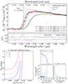 |
Fig. 14. Model of the Lyα break in the PRISM spectrum. Upper panel: Best fit (red line) from a model in which we attenuate a power-law spectrum by applying the transmission curve from a fully neutral IGM (xHI fixed to 1) while fitting for the size of any ionised bubble (Rion) surrounding GS-z9-0 and for the column density of a local DLA system along the line of sight (NHI). The residuals from the fit are compared with both the pipeline error spectrum and the square root of the diagonal terms of the covariance matrix described in Sect. 6 (Jakobsen et al., in prep.). The formal best-fit values provide Rion∼0 and log(NHI/cm−2) = 19.9. We note that including attenuation from the column density of neutral gas placed at the galaxy systemic redshift does not provide significant improvements to the model compared to only applying attenuation from purely neutral IGM (blue dotted line). For comparison, the light and dark green curves show the spectral shape obtained by including DLAs with log(NHI/cm−2) = 21.5 and 22.5, respectively. Bottom left panel: Contour levels of the χ2-map on the log(NHI) vs. Rion parameter space, highlighting 1σ, 2σ, and 3σ confidence regions. The column density of any DLA at the systemic redshift is constrained to log(NHI/cm−2) <20.75 at 99.7% confidence. Bottom right panel: Joint contours and marginalised posterior probability density function for the same parameters. The quoted upper limits report the 95th per centiles of the posterior distributions. |
Interestingly, our inferred upper limits are much lower than what other recent observations of z≳10 galaxies have suggested, reporting detection of local column densities of neutral gas as high as log(NHI/cm−2) = 22.5 which have been interpreted as evidence for the presence of large reservoirs of cold gas available to sustain early star formation and galaxy growth (e.g. D’Eugenio et al. 2024; Heintz et al. 2024, 2025; Hainline et al. 2024b; Carniani et al. 2024). Such large column densities would push the onset of the Lyα absorption trough redwards with respect to the systemic redshift and significantly soften the observed spectral break: this is illustrated for instance by the light and dark green curves in Fig. 14, which show how the transmitted spectrum would look in the presence of local DLAs of log(NHI/cm−2) = 21.5 and 22.5, respectively, resulting in very different spectral shapes than observed in the PRISM spectrum of GS-z9-0.
To test the amount of degeneracy between the column density of neutral gas in the CGM/ISM and the hydrogen neutral fraction in the IGM and its impact on the results of our fit, we have also performed a run by leaving also  free to vary between 0 and 1, finding that the fit still favours a solution with high
  (
( ), little Rion (
 pMpc), and low NHI (log(NHI/cm−2)
  ), which means that the transmission curve from the IGM absorption cannot be exactly mimicked by local ISM/CGM absorption in the form of a DLA component at any column density. We note that in such a scenario the inferred value for
  is slightly higher than (though consistent with) that measured by Umeda et al. (2024) on an average, stacked JWST/PRISM spectrum of z >9 galaxies. Furthermore, we have tested that only a fine-tuned model with the DLA component placed at a redshift z[DLA] ∼9.3 and large column density (log(NHI/cm−2) ≳22.3) can mimic the transmission curve of a fully neutral IGM (delivering a comparable goodness of fit), but this would likely imply the presence of a foreground system which is not seen in NIRCAM imaging (see also Jakobsen et al., in prep.).
For what concerns the constraints inferred from our simple model on the size of a possible ionised region around GS-z9-0, the bottom left panel of Fig. 14 shows that for any value of log(NHI/cm−2) ≲20 Rion is constrained to be ≲0.1 pMpc at 1σ confidence (≲0.4 pMpc at 3σ confidence), whereas only within a rather fine-tuned interval of log(NHI/cm−2) values (20.3≲ log(NHI/cm−2) ≲20.8) the 1σ confidence region extends up to 0.6 pMpc (with 2σ and 3σ intervals extending beyond 1 pMpc). Again, similar constraints are obtained from the marginalised posterior PDF for Rion, from which we quote Rion<0.447 pMpc as the 95th per centile of the distribution.
We can compare the constraints on Rion derived from our modelling of the Lyα spectral break with what we could expect for a galaxy such as GS-z9-0 on the basis of simple arguments involving the age of the system and its ionising efficiency. First, we estimated the ionising photons production efficiency of GS-z9-0 leveraging the measured flux of Hβ. We followed Saxena et al. (2023), Simmonds et al. (2023), Witstok et al. (2025b), among others, to infer

measuring the UV luminosity density at 1500 Å rest-frame and under the assumption of case B recombination and zero escape fraction of Lyman continuum photons (fesc, LyC = 0, hence yielding a lower limit), finding log(ξion/erg−1 Hz) = 25.64, in agreement with typical values for bright (MUV<−20) galaxies in the EoR (e.g. Endsley et al. 2024). Following Mason & Gronke (2020), Witstok et al. (2024), among others, we then estimated the size of the surrounding ionised region that would be produced by a galaxy similar to GS-z9-0 from
where  (z) is the mean hydrogen number density at redshift z and Ṅion the production rate of ionising photons. Assuming that the ionising photon production is powered by a very recent burst of star formation occurred over the past 5 Myr, as suggested by both the steeply rising SFH derived in Sect. 2.3 and the chemical abundance patterns discussed in Sect. 5, and a fesc, LyC = 5% (Finkelstein et al. 2019) would produce an ionised bubble with size Rion≈0.1 pMpc (0.05–0.12 pMpc if assuming fesc, LyC ranging between 1% and 10%), in good agreement with the 1σ confidence limits inferred from our modelling of the Lyα break for the majority of allowed NHI values. These values are also in line with what predicted for Lyα emitters (LAEs) with similar physical properties to GS-z9-0 discovered at slightly lower redshift (see e.g. ∼7−8 objects in Witstok et al. 2024, 2025b), whose (sometimes significantly) larger inferred sizes of ionised bubbles (constrained by large observed Lyα/Hβ ratios and small velocity offsets) require including the contribution from either faint neighbour companions or older galaxies, to assume bursty SFHs, or to invoke particularly favourable geometrical configurations.
Summarising, we find indications for GS-z9-0 to be surrounded by a small ionised bubble, as suggested by the low escape fraction of Lyα photons (∼1%), the relatively large velocity offset (∼450 km/s), and the constraints set by modelling the damping wing of the Lyα break. Despite the high production efficiency of ionising photons powered by its recent SFH, this galaxy is therefore unlikely to have contributed significantly to reionisation at the epoch of observations. Nonetheless, it is possible that the presence of outflowing gas (as also suggested by the velocity shift observed in the C IV emission) is helping to create channels through which Lyα photons can escape from a fully neutral IGM; the presence of such outflows has been suggested as almost ubiquitous in early galaxies with high sSFR (Ferrara 2024; Ferrara et al. 2025).
Finally, we note that, despite providing a reasonably good match to the data, our simplified baseline model assuming  = 1 is not capable of perfectly reproducing the observed spectral shape of GS-z9-0 in the PRISM spectrum, as clear residuals are observed for instance between ∼1.3–1.35 μm, where the profile softens before turning-over (see Fig. 14). We note that in order to place more stringent constraints on the neutral fraction of the IGM it is critical to have a better understanding of the systematics involved in modelling the intrinsic UV continuum and the exact shape of the Lyα emission that emerges from the galaxy, as well as the impact of possible fluctuations in the hydrogen density associated with large-scale structures at these redshifts (e.g. Smith et al. 2022). Moreover, a proper modelling of the contribution to attenuation due to local absorbers would require the precise knowledge of the geometry and density profiles of the intervening gas clouds (Gronke 2017; Hutter et al. 2023). A more detailed discussion on the damping wing of the Lyα absorption profile in GS-z9-0, the inferred constraints on x
 , and the implications on the history of cosmic reionisation, is presented in Jakobsen et al., (in prep.).
7. Summary
We have presented ultra-deep JWST/NIRSpec observations of GS-z9-0, a luminous (MUV=−20.43) galaxy at redshift z∼9.4327. Combining datasets from JADES programmes PID 1210 and PID 3215 provided a total of 72 hours of observations in PRISM/CLEAR mode, 44 hours in G395M/F290LP mode, and 16 hours in G140M/F070LP mode. Leveraging the high signal-to-noise ratio of the spectrum (Fig. 2) and the detection of multiple emission lines in the rest-frame optical and UV regimes (Figs. 3 and 5), we characterised the ISM properties and the star formation history of this source, observed only ∼500 Myr after the Big Bang.
The main results discussed in the paper are summarised as follows:
-
The system is young (light-weighted age ∼3 Myr, mass-weighted age of ∼30 Myr) and compact (Re∼110 pc), and exhibits a steeply rising star formation history over the past 3–10 Myr with high star formation rate surface density (ΣSFR∼72 M⊙ yr−1 kpc−2), suggesting that the majority of mass assembly occurred during a recent and concentrated burst of star formation (Fig. 6). Negligible dust attenuation is inferred from both SED fitting and Balmer lines (Fig. 7).
-
Emission line ratios from the rest-frame UV are indicative of a hard radiation field powered by young, massive, and metal-poor stars (Fig. 8), in particular when the abundance patterns of the model grids (e.g. in C/O) are matched to those inferred independently from the emission lines. However, the tentative detection of the extremely high-ionisation [Ne V] λ3426 line (Fig. 3) suggests that a contribution to ionisation from the NLR of an AGN or from shocks driven by SN explosions cannot be excluded (Fig. 9).
-
The measured C/O abundance (log(C/O) =−0.90, [C/O] =−0.64) lies at the lowest envelope of the distribution of local and high-redshift galaxies at similar metallicity (12 + log(O/H) ∼7.5), in agreement with a rapid recent history of chemical enrichment dominated by yields of core-collapse supernovae from massive stars progenitors (Fig. 11).
-
However, the detection of N III] λ1750 emission in the PRISM spectrum suggests low C/N and hence overabundant N/O (log(N/O) =−0.93, [N/O] =−0.07) compared to the average plateau occupied by local low-metallicity galaxies, similar to (though not as extreme as) the nitrogen-enriched galaxies at z>6 recently observed by JWST (Fig. 11). This is also corroborated by the marginal detection of N IV] λ1483 in the 3 pixel extracted G140M spectrum.
-
The observed CNO abundance patterns are well reproduced by single-burst chemical evolution models including a contribution from very massive stars (M★≳100 M⊙), possibly revealing the short timescale signatures of enrichment from Wolf-Rayet stars or pair-instability supernovae progenitors, in line with a top-heavy IMF scenario regulating the process of star formation in the earliest galaxies (Fig. 12). More fine-tuned SFHs (e.g. characterised by two bursts separated by a ∼100 Myr period of quiescence) are required to match the CNO abundance patterns assuming a standard IMF.
-
By modelling the Lyα spectral break under the assumption of a fully neutral IGM, we rule out the presence of very high column density local absorbers (log(NHI/cm−2) ≲20.75 at 99.7% confidence; Fig. 14). We also report the tentative detection of Lyα emission in the G140M spectrum (Fig. 13), redshifted by ∼450 km/s from systemic, from which we infer an escape fraction of Lyα photons from IGM attenuation of ∼1%. Together with the constraints from the Lyα break, and in line with the young age of the system, this suggests the size of any ionised region surrounding GS-z9-0 to be ≲0.1–0.2 pMpc and that, despite the high production efficiency of ionising photons, this system had not yet significantly contributed to cosmic reionisation at the time of observations.
Sources such as GS-z9-0 currently represent the best opportunities to directly investigate the physics underlying the early phases of galaxy assembly, their evolution, and the environment they live in. The richness of spectral features and the peculiar chemical abundances observed in this and other high-redshift systems challenge our understanding of the nature of massive stars powering the extreme emission lines seen in the spectra, and possibly hint at the role of early accretion onto (super-)massive black holes. In this sense, the present analysis also highlights the wealth of information delivered by deep observations that simultaneously probe rest-frame UV and optical spectra of z∼6–10 galaxies. However, despite the enormous advancements already brought by JWST, the intrinsic faintness of most rest-frame UV stellar and nebular features currently hinders their detailed characterisation within the context of the more general high-redshift galaxy population. Alongside the identification and follow-up of new bright high-redshift candidates, deeper spectroscopy at medium to high resolution probing the UV continuum and emission line features over large samples will therefore be the key to gradually move from the study of the most luminous systems towards a broader understanding of the physical properties of galaxies in the early Universe.
Acknowledgments
We thank the anonymous referee for the insightful comments that contributed to strengthen the analysis and improved the clarity of the paper. We are grateful to Danielle Berg, Matilde Mingozzi, Anna Feltre, Bethan James, John Chisholm, Evan Skillman, Alessandro Marconi, Charles Steidel, Andrea Ferrara, and Jorick Vink for enlightening conversations. MC acknowledges support by the European Southern Observatory (ESO) Fellowship Programme. JW, FDE, RM, JS, & WB acknowledge support by the Science and Technology Facilities Council (STFC), ERC Advanced Grant 695671 “QUENCH”, and by the UKRI Frontier Research grant RISEandFALL. RM also acknowledges funding from a research professorship from the Royal Society. The Cosmic Dawn Center (DAWN) is funded by the Danish National Research Foundation under grant DNRF140. ECL acknowledges support of an STFC Webb Fellowship (ST/W001438/1). JC, AJB & AC acknowledge funding from the “FirstGalaxies” Advanced Grant from the European Research Council (ERC) under the European Union's Horizon 2020 research and innovation programme (Grant agreement No. 789056). SC & GV acknowledge support by European Union's HE ERC Starting Grant No. 101040227 – WINGS. SA acknowledges grant PID2021-127718NB-I00 funded by the Spanish Ministry of Science and Innovation/State Agency of Research (MICIN/AEI/ 10.13039/501100011033). This research is supported in part by the Australian Research Council Centre of Excellence for All Sky Astrophysics in 3 Dimensions (ASTRO 3D), through project number CE170100013. DJE, BDJ, BR, and CNAW are supported by JWST/NIRCam contract to the University of Arizona NAS5-02015. DJE is also supported as a Simons Investigator. BER acknowledges support from the NIRCam Science Team contract to the University of Arizona, NAS5-02015, and JWST Program 3215. ST acknowledges support by the Royal Society Research Grant G125142. HÜ gratefully acknowledges support by the Isaac Newton Trust and by the Kavli Foundation through a Newton-Kavli Junior Fellowship. The research of CCW is supported by NOIRLab, which is managed by the Association of Universities for Research in Astronomy (AURA) under a cooperative agreement with the National Science Foundation.
This ICF is larger than that inferred from the relations presented in Amayo et al. (2021) (i.e. ICF = 1.05). Instead, feeding the ICF equations from Berg et al. (2019b) with the higher log(U) values derived from SED fitting from both BEAGLE (log(U) =−1.46) and BAGPIPES (log(U) =−1.05), although not based on self-consistently generated CLOUDY grids, would translate into ICF = 1.45 and ICF = 2, and hence into higher log(C/O) =−0.80±0.11 and log(C/O) =−0.65±0.11, respectively.
Which is derived by combining C/N and C/O; Sect. 4.4.
We note that while such a weak Lyα line is not expected to be seen directly at the PRISM resolution, where it becomes fully blended with the break, it does affect its spectral shape, e.g. Jones et al. (2024).
Our likelihood model includes the covariance matrix as in Eq. (2), and we assume flat linear prior on log(NHI/cm−2), while log-uniform prior on Rion between linear values of 10−2 and 100.5.
References
- Akerman, C. J., Carigi, L., Nissen, P. E., Pettini, M., & Asplund, M. 2004, A&A, 414, 931 [NASA ADS] [CrossRef] [EDP Sciences] [Google Scholar]
- Alexander, R. K., Vincenzo, F., Ji, A. P., et al. 2023, MNRAS, 522, 5415 [Google Scholar]
- Amayo, A., Delgado-Inglada, G., & Stasińska, G. 2021, MNRAS, 505, 2361 [CrossRef] [Google Scholar]
- Amorín, R., Fontana, A., Pérez-Montero, E., et al. 2017, Nat. Astron., 1, 0052 [Google Scholar]
- Arellano-Córdova, K. Z., Berg, D. A., Chisholm, J., et al. 2022, ApJ, 940, L23 [CrossRef] [Google Scholar]
- Arrabal Haro, P., Dickinson, M., Finkelstein, S. L., et al. 2023, Nature, 622, 707 [NASA ADS] [CrossRef] [Google Scholar]
- Asplund, M., Grevesse, N., Sauval, A. J., & Scott, P. 2009, ARA&A, 47, 481 [NASA ADS] [CrossRef] [Google Scholar]
- Backhaus, B. E., Trump, J. R., Cleri, N. J., et al. 2022, ApJ, 926, 161 [NASA ADS] [CrossRef] [Google Scholar]
- Baker, W. M., Tacchella, S., Johnson, B. D., et al. 2025, Nat. Astron., 9, 141 [Google Scholar]
- Batra, N. D., & Baldwin, J. A. 2014, MNRAS, 439, 771 [NASA ADS] [CrossRef] [Google Scholar]
- Bayliss, M. B., Rigby, J. R., Sharon, K., et al. 2014, ApJ, 790, 144 [NASA ADS] [CrossRef] [Google Scholar]
- Belokurov, V., & Kravtsov, A. 2023, MNRAS, 525, 4456 [NASA ADS] [CrossRef] [Google Scholar]
- Benjamin, R. A., Skillman, E. D., & Smits, D. P. 1999, ApJ, 514, 307 [Google Scholar]
- Berg, D. A., Skillman, E. D., Marble, A. R., et al. 2012, ApJ, 754, 98 [NASA ADS] [CrossRef] [Google Scholar]
- Berg, D. A., Skillman, E. D., Croxall, K. V., et al. 2015, ApJ, 806, 16 [NASA ADS] [CrossRef] [Google Scholar]
- Berg, D. A., Skillman, E. D., Henry, R. B. C., Erb, D. K., & Carigi, L. 2016, ApJ, 827, 126 [NASA ADS] [CrossRef] [Google Scholar]
- Berg, D. A., Erb, D. K., Auger, M. W., Pettini, M., & Brammer, G. B. 2018, ApJ, 859, 164 [CrossRef] [Google Scholar]
- Berg, D. A., Chisholm, J., Erb, D. K., et al. 2019a, ApJ, 878, L3 [NASA ADS] [CrossRef] [Google Scholar]
- Berg, D. A., Erb, D. K., Henry, R. B. C., Skillman, E. D., & McQuinn, K. B. W. 2019b, ApJ, 874, 93 [NASA ADS] [CrossRef] [Google Scholar]
- Berg, D. A., Pogge, R. W., Skillman, E. D., et al. 2020, ApJ, 893, 96 [NASA ADS] [CrossRef] [Google Scholar]
- Berg, D. A., Chisholm, J., Erb, D. K., et al. 2021, ApJ, 922, 170 [CrossRef] [Google Scholar]
- Berg, D. A., James, B. L., King, T., et al. 2022, ApJS, 261, 31 [NASA ADS] [CrossRef] [Google Scholar]
- Binette, L., Matadamas, R., Hägele, G. F., et al. 2012, A&A, 547, A29 [NASA ADS] [CrossRef] [EDP Sciences] [Google Scholar]
- Bouwens, R. J., Stefanon, M., Oesch, P. A., et al. 2019, ApJ, 880, 25 [NASA ADS] [CrossRef] [Google Scholar]
- Boyett, K., Bunker, A. J., Curtis-Lake, E., et al. 2024, MNRAS, 535, 1796 [NASA ADS] [CrossRef] [Google Scholar]
- Brinchmann, J. 2023, MNRAS, 525, 2087 [NASA ADS] [CrossRef] [Google Scholar]
- Bunker, A. J., Saxena, A., Cameron, A. J., et al. 2023, A&A, 677, A88 [NASA ADS] [CrossRef] [EDP Sciences] [Google Scholar]
- Bunker, A. J., Cameron, A. J., Curtis-Lake, E., et al. 2024, A&A, 690, A288 [NASA ADS] [CrossRef] [EDP Sciences] [Google Scholar]
- Byler, N., Dalcanton, J. J., Conroy, C., & Johnson, B. D. 2017, ApJ, 840, 44 [Google Scholar]
- Calabrò, A., Castellano, M., Zavala, J. A., et al. 2024, ApJ, 975, 245 [CrossRef] [Google Scholar]
- Calzetti, D., Armus, L., Bohlin, R. C., et al. 2000, ApJ, 533, 682 [NASA ADS] [CrossRef] [Google Scholar]
- Cameron, A. J., Saxena, A., Bunker, A. J., et al. 2023a, A&A, 677, A115 [NASA ADS] [CrossRef] [EDP Sciences] [Google Scholar]
- Cameron, A. J., Katz, H., Rey, M. P., & Saxena, A. 2023b, MNRAS, 523, 3516 [NASA ADS] [CrossRef] [Google Scholar]
- Campbell, A., Terlevich, R., & Melnick, J. 1986, MNRAS, 223, 811 [NASA ADS] [CrossRef] [Google Scholar]
- Cappellari, M. 2017, MNRAS, 466, 798 [Google Scholar]
- Carnall, A. C., McLure, R. J., Dunlop, J. S., & Davé, R. 2018, MNRAS, 480, 4379 [Google Scholar]
- Carniani, S., Hainline, K., D’Eugenio, F., et al. 2024, Nature, 633, 318 [CrossRef] [Google Scholar]
- Carretta, E., Gratton, R. G., Lucatello, S., Bragaglia, A., & Bonifacio, P. 2005, A&A, 433, 597 [NASA ADS] [CrossRef] [EDP Sciences] [Google Scholar]
- Castellano, M., Napolitano, L., Fontana, A., et al. 2024, ApJ, 972, 143 [Google Scholar]
- Chabrier, G. 2003, PASP, 115, 763 [Google Scholar]
- Charbonnel, C., Schaerer, D., Prantzos, N., et al. 2023, A&A, 673, L7 [NASA ADS] [CrossRef] [EDP Sciences] [Google Scholar]
- Charlot, S., & Fall, S. M. 2000, ApJ, 539, 718 [Google Scholar]
- Chemerynska, I., Atek, H., Furtak, L. J., et al. 2024, MNRAS, 531, 2615 [NASA ADS] [CrossRef] [Google Scholar]
- Chevallard, J., & Charlot, S. 2016, MNRAS, 462, 1415 [NASA ADS] [CrossRef] [Google Scholar]
- Chiappini, C., Hirschi, R., Meynet, G., et al. 2006, A&A, 449, L27 [NASA ADS] [CrossRef] [EDP Sciences] [Google Scholar]
- Chisholm, J., Berg, D. A., Endsley, R., et al. 2024, MNRAS, 534, 2633 [NASA ADS] [CrossRef] [Google Scholar]
- Christensen, L., Laursen, P., Richard, J., et al. 2012, MNRAS, 427, 1973 [NASA ADS] [CrossRef] [Google Scholar]
- Clarke, L., Shapley, A. E., Sanders, R. L., et al. 2024, ApJ, 977, 133 [NASA ADS] [CrossRef] [Google Scholar]
- Cleri, N. J., Olivier, G. M., Hutchison, T. A., et al. 2023, ApJ, 953, 10 [NASA ADS] [CrossRef] [Google Scholar]
- Cooke, R. J., Pettini, M., & Steidel, C. C. 2017, MNRAS, 467, 802 [NASA ADS] [Google Scholar]
- Croxall, K. V., Pogge, R. W., Berg, D. A., Skillman, E. D., & Moustakas, J. 2016, ApJ, 830, 4 [NASA ADS] [CrossRef] [Google Scholar]
- Curti, M., Maiolino, R., Curtis-Lake, E., et al. 2024, A&A, 684, A75 [NASA ADS] [CrossRef] [EDP Sciences] [Google Scholar]
- Curtis-Lake, E., Carniani, S., Cameron, A., et al. 2023, Nat. Astron., 7, 622 [NASA ADS] [CrossRef] [Google Scholar]
- de Graaff, A., Rix, H. -W., Carniani, S., et al. 2024, A&A, 684, A87 [NASA ADS] [CrossRef] [EDP Sciences] [Google Scholar]
- D’Eugenio, F., Maiolino, R., Carniani, S., et al. 2024, A&A, 689, A152 [NASA ADS] [CrossRef] [EDP Sciences] [Google Scholar]
- D’Eugenio, F., Cameron, A. J., Scholtz, J., et al. 2025, ApJS, 277, 4 [Google Scholar]
- Dijkstra, M. 2014, PASA, 31, e040 [Google Scholar]
- D’Orazi, V., Lucatello, S., Gratton, R., et al. 2010, ApJ, 713, L1 [Google Scholar]
- Dors, O. L., Maiolino, R., Cardaci, M. V., et al. 2020, MNRAS, 496, 3209 [NASA ADS] [CrossRef] [Google Scholar]
- Dors, O. L., Valerdi, M., Freitas-Lemes, P., et al. 2022, MNRAS, 514, 5506 [NASA ADS] [CrossRef] [Google Scholar]
- Dressler, A., Vulcani, B., Treu, T., et al. 2023, ApJ, 947, L27 [NASA ADS] [CrossRef] [Google Scholar]
- Eisenstein, D. J., Willott, C., Alberts, S., et al. 2023a, ApJ, submitted [arXiv:2306.02465] [Google Scholar]
- Eisenstein, D. J., Johnson, B. D., Robertson, B., et al. 2023b, ApJ, submitted [arXiv:2310.12340] [Google Scholar]
- Endsley, R., Stark, D. P., Whitler, L., et al. 2024, MNRAS, 533, 1111 [NASA ADS] [CrossRef] [Google Scholar]
- Erb, D. K., Pettini, M., Shapley, A. E., et al. 2010, ApJ, 719, 1168 [Google Scholar]
- Esteban, C., Peimbert, M., García-Rojas, J., et al. 2004, MNRAS, 355, 229 [NASA ADS] [CrossRef] [Google Scholar]
- Esteban, C., Bresolin, F., Peimbert, M., et al. 2009, ApJ, 700, 654 [NASA ADS] [CrossRef] [Google Scholar]
- Esteban, C., García-Rojas, J., Carigi, L., et al. 2014, MNRAS, 443, 624 [NASA ADS] [CrossRef] [Google Scholar]
- Esteban, C., Fang, X., García-Rojas, J., & Toribio San Cipriano, L. 2017, MNRAS, 471, 987 [NASA ADS] [CrossRef] [Google Scholar]
- Fabbian, D., Nissen, P. E., Asplund, M., Pettini, M., & Akerman, C. 2009, A&A, 500, 1143 [NASA ADS] [CrossRef] [EDP Sciences] [Google Scholar]
- Feltre, A., Charlot, S., & Gutkin, J. 2016, MNRAS, 456, 3354 [Google Scholar]
- Ferland, G. J., Chatzikos, M., Guzmán, F., et al. 2017, Rev. Mex. Astron. Astrofis., 53, 385 [NASA ADS] [Google Scholar]
- Feroz, F., Hobson, M. P., & Bridges, M. 2009, MNRAS, 398, 1601 [NASA ADS] [CrossRef] [Google Scholar]
- Ferrara, A. 2024, A&A, 684, A207 [NASA ADS] [CrossRef] [EDP Sciences] [Google Scholar]
- Ferrara, A., Pallottini, A., & Dayal, P. 2023, MNRAS, 522, 3986 [NASA ADS] [CrossRef] [Google Scholar]
- Ferrara, A., Pallottini, A., & Sommovigo, L. 2025, A&A, 694, A286 [NASA ADS] [CrossRef] [EDP Sciences] [Google Scholar]
- Finkelstein, S. L., D’Aloisio, A., Paardekooper, J. -P., et al. 2019, ApJ, 879, 36 [NASA ADS] [CrossRef] [Google Scholar]
- Fosbury, R. A. E., Villar-Martín, M., Humphrey, A., et al. 2003, ApJ, 596, 797 [NASA ADS] [CrossRef] [Google Scholar]
- García-Rojas, J., & Esteban, C. 2007, ApJ, 670, 457 [CrossRef] [Google Scholar]
- García-Rojas, J., Esteban, C., Peimbert, M., et al. 2004, ApJS, 153, 501 [CrossRef] [Google Scholar]
- García-Rojas, J., Esteban, C., Peimbert, A., et al. 2005, MNRAS, 362, 301 [CrossRef] [Google Scholar]
- García-Rojas, J., Esteban, C., Peimbert, A., et al. 2007, Rev. Mex. Astron. Astrofis., 43, 3 [Google Scholar]
- Garnett, D. R. 1992, AJ, 103, 1330 [NASA ADS] [CrossRef] [Google Scholar]
- Gilli, R., Vignali, C., Mignoli, M., et al. 2010, A&A, 519, A92 [NASA ADS] [CrossRef] [EDP Sciences] [Google Scholar]
- Gordon, K. D., Clayton, G. C., Misselt, K. A., Landolt, A. U., & Wolff, M. J. 2003, ApJ, 594, 279 [NASA ADS] [CrossRef] [Google Scholar]
- Greene, J. E., Labbe, I., Goulding, A. D., et al. 2024, ApJ, 964, 39 [CrossRef] [Google Scholar]
- Gronke, M. 2017, A&A, 608, A139 [NASA ADS] [CrossRef] [EDP Sciences] [Google Scholar]
- Groves, B. A., Dopita, M. A., & Sutherland, R. S. 2004, ApJS, 153, 75 [NASA ADS] [CrossRef] [Google Scholar]
- Gunn, J. E., & Peterson, B. A. 1965, ApJ, 142, 1633 [Google Scholar]
- Gustafsson, B., Karlsson, T., Olsson, E., Edvardsson, B., & Ryde, N. 1999, A&A, 342, 426 [NASA ADS] [Google Scholar]
- Gutkin, J., Charlot, S., & Bruzual, G. 2016, MNRAS, 462, 1757 [Google Scholar]
- Hägele, G. F., Pérez-Montero, E., Díaz, Á. I., Terlevich, E., & Terlevich, R. 2006, MNRAS, 372, 293 [CrossRef] [Google Scholar]
- Hainline, K. N., Johnson, B. D., Robertson, B., et al. 2024a, ApJ, 964, 71 [CrossRef] [Google Scholar]
- Hainline, K. N., D’Eugenio, F., Jakobsen, P., et al. 2024b, ApJ, 976, 160 [NASA ADS] [CrossRef] [Google Scholar]
- Harikane, Y., Zhang, Y., Nakajima, K., et al. 2023, ApJ, 959, 39 [NASA ADS] [CrossRef] [Google Scholar]
- Harikane, Y., Nakajima, K., Ouchi, M., et al. 2024, ApJ, 960, 56 [NASA ADS] [CrossRef] [Google Scholar]
- Heintz, K. E., Watson, D., Brammer, G., et al. 2024, Science, 384, 890 [NASA ADS] [CrossRef] [Google Scholar]
- Heintz, K. E., Brammer, G. B., Watson, D., et al. 2025, A&A, 693, A60 [Google Scholar]
- Hirschmann, M., Charlot, S., Feltre, A., et al. 2019, MNRAS, 487, 333 [NASA ADS] [CrossRef] [Google Scholar]
- Holwerda, B. W., Bouwens, R., Oesch, P., et al. 2015, ApJ, 808, 6 [CrossRef] [Google Scholar]
- Hutchison, T. A., Papovich, C., Finkelstein, S. L., et al. 2019, ApJ, 879, 70 [NASA ADS] [CrossRef] [Google Scholar]
- Hutter, A., Trebitsch, M., Dayal, P., et al. 2023, MNRAS, 524, 6124 [NASA ADS] [CrossRef] [Google Scholar]
- Iani, E., Zanella, A., Vernet, J., et al. 2023, MNRAS, 518, 5018 [Google Scholar]
- Inoue, A. K., Shimizu, I., Iwata, I., & Tanaka, M. 2014, MNRAS, 442, 1805 [NASA ADS] [CrossRef] [Google Scholar]
- Isobe, Y., Ouchi, M., Tominaga, N., et al. 2023a, ApJ, 959, 100 [NASA ADS] [CrossRef] [Google Scholar]
- Isobe, Y., Ouchi, M., Nakajima, K., et al. 2023b, ApJ, 956, 139 [NASA ADS] [CrossRef] [Google Scholar]
- Izotov, Y. I. 2006, in Stellar Evolution at Low Metallicity: Mass Loss, Explosions, Cosmology, eds. H. J. G. L. M. Lamers, N. Langer, T. Nugis, & K. Annuk, ASP Conf. Ser., 353, 349 [Google Scholar]
- Izotov, Y. I., Stasińska, G., Meynet, G., Guseva, N. G., & Thuan, T. X. 2006, A&A, 448, 955 [CrossRef] [EDP Sciences] [Google Scholar]
- Izotov, Y. I., Thuan, T. X., & Privon, G. 2012, MNRAS, 427, 1229 [NASA ADS] [CrossRef] [Google Scholar]
- Izotov, Y. I., Schaerer, D., Guseva, N. G., Thuan, T. X., & Worseck, G. 2024, MNRAS, 528, L10 [Google Scholar]
- James, B. L., Pettini, M., Christensen, L., et al. 2014, MNRAS, 440, 1794 [NASA ADS] [CrossRef] [Google Scholar]
- Ji, X., Übler, H., Maiolino, R., et al. 2024a, MNRAS, 535, 881 [NASA ADS] [CrossRef] [Google Scholar]
- Ji, X., Maiolino, R., Ferland, G., et al. 2024b, MNRAS, submitted [arXiv:2405.05772] [Google Scholar]
- Jones, T., Sanders, R., Chen, Y., et al. 2023, ApJ, 951, L17 [CrossRef] [Google Scholar]
- Jones, G. C., Bunker, A. J., Saxena, A., et al. 2024, A&A, 683, A238 [NASA ADS] [CrossRef] [EDP Sciences] [Google Scholar]
- Kobayashi, C., & Ferrara, A. 2024, ApJ, 962, L6 [NASA ADS] [CrossRef] [Google Scholar]
- Kobayashi, C., & Taylor, P. 2023, ArXiv e-prints [arXiv:2302.07255] [Google Scholar]
- Kobayashi, C., Karakas, A. I., & Umeda, H. 2011, MNRAS, 414, 3231 [Google Scholar]
- Kobayashi, C., Karakas, A. I., & Lugaro, M. 2020, ApJ, 900, 179 [Google Scholar]
- Kokorev, V., Caputi, K. I., Greene, J. E., et al. 2024, ApJ, 968, 38 [NASA ADS] [CrossRef] [Google Scholar]
- Kroupa, P. 2008, in Pathways Through an Eclectic Universe, eds. J. H. Knapen, T. J. Mahoney, & A. Vazdekis, ASP Conf. Ser., 390, 3 [Google Scholar]
- Langeroodi, D., & Hjorth, J. 2023, ArXiv e-prints [arXiv:2307.06336] [Google Scholar]
- Laseter, I. H., Maseda, M. V., Curti, M., et al. 2024, A&A, 681, A70 [NASA ADS] [CrossRef] [EDP Sciences] [Google Scholar]
- Lecroq, M., Charlot, S., Bressan, A., et al. 2024, MNRAS, 527, 9480 [Google Scholar]
- Leitherer, C., Tremonti, C. A., Heckman, T. M., & Calzetti, D. 2011, AJ, 141, 37 [NASA ADS] [CrossRef] [Google Scholar]
- Leja, J., Carnall, A. C., Johnson, B. D., Conroy, C., & Speagle, J. S. 2019, ApJ, 876, 3 [Google Scholar]
- Looser, T. J., D’Eugenio, F., Maiolino, R., et al. 2025, A&A, 697, A88 [NASA ADS] [CrossRef] [EDP Sciences] [Google Scholar]
- López-Sánchez, Á. R., Esteban, C., García-Rojas, J., Peimbert, M., & Rodríguez, M. 2007, ApJ, 656, 168 [CrossRef] [Google Scholar]
- Mainali, R., Kollmeier, J. A., Stark, D. P., et al. 2017, ApJ, 836, L14 [Google Scholar]
- Mainali, R., Stark, D. P., Tang, M., et al. 2020, MNRAS, 494, 719 [NASA ADS] [CrossRef] [Google Scholar]
- Maiolino, R., & Mannucci, F. 2019, A&ARv, 27, 3 [Google Scholar]
- Maiolino, R., Scholtz, J., Curtis-Lake, E., et al. 2024a, A&A, 691, A145 [NASA ADS] [CrossRef] [EDP Sciences] [Google Scholar]
- Maiolino, R., Scholtz, J., Witstok, J., et al. 2024b, Nature, 627, 59 [NASA ADS] [CrossRef] [Google Scholar]
- Marconi, A., Amiri, A., Feltre, A., et al. 2024, A&A, 689, A78 [NASA ADS] [CrossRef] [EDP Sciences] [Google Scholar]
- Marques-Chaves, R., Schaerer, D., Kuruvanthodi, A., et al. 2024, A&A, 681, A30 [NASA ADS] [CrossRef] [EDP Sciences] [Google Scholar]
- Maseda, M. V., Lewis, Z., Matthee, J., et al. 2023, ApJ, 956, 11 [NASA ADS] [CrossRef] [Google Scholar]
- Mason, C. A., & Gronke, M. 2020, MNRAS, 499, 1395 [Google Scholar]
- Mason, C. A., Trenti, M., & Treu, T. 2023, MNRAS, 521, 497 [NASA ADS] [CrossRef] [Google Scholar]
- Matteucci, F. 1986, MNRAS, 221, 911 [NASA ADS] [Google Scholar]
- Matthee, J., Sobral, D., Hayes, M., et al. 2021, MNRAS, 505, 1382 [NASA ADS] [CrossRef] [Google Scholar]
- Matthee, J., Naidu, R. P., Brammer, G., et al. 2024, ApJ, 963, 129 [NASA ADS] [CrossRef] [Google Scholar]
- McLeod, D. J., Donnan, C. T., McLure, R. J., et al. 2024, MNRAS, 527, 5004 [Google Scholar]
- Méndez-Delgado, J. E., Esteban, C., García-Rojas, J., et al. 2023a, MNRAS, 523, 2952 [CrossRef] [Google Scholar]
- Méndez-Delgado, J. E., Esteban, C., García-Rojas, J., Kreckel, K., & Peimbert, M. 2023b, Nature, 618, 249 [CrossRef] [Google Scholar]
- Mignoli, M., Vignali, C., Gilli, R., et al. 2013, A&A, 556, A29 [NASA ADS] [CrossRef] [EDP Sciences] [Google Scholar]
- Mingozzi, M., James, B. L., Berg, D. A., et al. 2024, ApJ, 962, 95 [Google Scholar]
- Nagele, C., & Umeda, H. 2023, ApJ, 949, L16 [NASA ADS] [CrossRef] [Google Scholar]
- Nakajima, K., Ouchi, M., Isobe, Y., et al. 2023, ApJS, 269, 33 [NASA ADS] [CrossRef] [Google Scholar]
- Nandal, D., Sibony, Y., & Tsiatsiou, S. 2024, A&A, 688, A142 [NASA ADS] [CrossRef] [EDP Sciences] [Google Scholar]
- Napolitano, L., Castellano, M., Pentericci, L., et al. 2024, ApJ, Submitted [arXiv:2410.18763] [Google Scholar]
- Nissen, P. E., Chen, Y. Q., Carigi, L., Schuster, W. J., & Zhao, G. 2014, A&A, 568, A25 [NASA ADS] [CrossRef] [EDP Sciences] [Google Scholar]
- Oesch, P. A., Bouwens, R. J., Illingworth, G. D., et al. 2014, ApJ, 786, 108 [Google Scholar]
- Oesch, P. A., Brammer, G., Naidu, R. P., et al. 2023, MNRAS, 525, 2864 [NASA ADS] [CrossRef] [Google Scholar]
- Peimbert, M., & Costero, R. 1969, BOTT, 5, 3 [Google Scholar]
- Peimbert, A., Peimbert, M., & Ruiz, M. T. 2005, ApJ, 634, 1056 [NASA ADS] [CrossRef] [Google Scholar]
- Pérez-Montero, E., & Amorín, R. 2017, MNRAS, 467, 1287 [Google Scholar]
- Pérez-Montero, E., & Contini, T. 2009, MNRAS, 398, 949 [CrossRef] [Google Scholar]
- Pilyugin, L. S., Mattsson, L., Vílchez, J. M., & Cedrés, B. 2009, MNRAS, 398, 485 [NASA ADS] [CrossRef] [Google Scholar]
- Planck Collaboration VI. 2020, A&A, 641, A6 [NASA ADS] [CrossRef] [EDP Sciences] [Google Scholar]
- Plat, A., Charlot, S., Bruzual, G., et al. 2019, MNRAS, 490, 978 [Google Scholar]
- Reddy, N. A., Topping, M. W., Shapley, A. E., et al. 2022, ApJ, 926, 31 [NASA ADS] [CrossRef] [Google Scholar]
- Reddy, N. A., Topping, M. W., Sanders, R. L., Shapley, A. E., & Brammer, G. 2023, ApJ, 952, 167 [CrossRef] [Google Scholar]
- Revalski, M., Rafelski, M., Henry, A., et al. 2024, ApJ, 966, 228 [Google Scholar]
- Rigby, J. R., Florian, M., Acharyya, A., et al. 2021, ApJ, 908, 154 [NASA ADS] [CrossRef] [Google Scholar]
- Robertson, B. E., Tacchella, S., Johnson, B. D., et al. 2023, Nat. Astron., 7, 611 [NASA ADS] [CrossRef] [Google Scholar]
- Robertson, B., Johnson, B. D., Tacchella, S., et al. 2024, ApJ, 970, 31 [NASA ADS] [CrossRef] [Google Scholar]
- Rogers, N. S. J., Skillman, E. D., Pogge, R. W., et al. 2021, ApJ, 915, 21 [NASA ADS] [CrossRef] [Google Scholar]
- Saccardi, A., Salvadori, S., D’Odorico, V., et al. 2023, ApJ, 948, 35 [NASA ADS] [CrossRef] [Google Scholar]
- Sanders, R. L., Shapley, A. E., Topping, M. W., Reddy, N. A., & Brammer, G. B. 2023, ApJ, 955, 54 [NASA ADS] [CrossRef] [Google Scholar]
- Saxena, A., Robertson, B. E., Bunker, A. J., et al. 2023, A&A, 678, A68 [NASA ADS] [CrossRef] [EDP Sciences] [Google Scholar]
- Schaerer, D., Marques-Chaves, R., Xiao, M., & Korber, D. 2024, A&A, 687, L11 [NASA ADS] [CrossRef] [EDP Sciences] [Google Scholar]
- Scholtz, J., Maiolino, R., D’Eugenio, F., et al. 2025, A&A, in press, https://doi.org/10.1051/0004-6361/202348804 [Google Scholar]
- Senchyna, P., Stark, D. P., Vidal-García, A., et al. 2017, MNRAS, 472, 2608 [NASA ADS] [CrossRef] [Google Scholar]
- Senchyna, P., Stark, D. P., Charlot, S., et al. 2022, ApJ, 930, 105 [NASA ADS] [CrossRef] [Google Scholar]
- Senchyna, P., Plat, A., Stark, D. P., et al. 2024, ApJ, 966, 92 [NASA ADS] [CrossRef] [Google Scholar]
- Shapley, A. E., Sanders, R. L., Reddy, N. A., Topping, M. W., & Brammer, G. B. 2023a, ApJ, 954, 157 [NASA ADS] [CrossRef] [Google Scholar]
- Shapley, A. E., Reddy, N. A., Sanders, R. L., Topping, M. W., & Brammer, G. B. 2023b, ApJ, 950, L1 [NASA ADS] [CrossRef] [Google Scholar]
- Simmonds, C., Tacchella, S., Maseda, M., et al. 2023, MNRAS, 523, 5468 [NASA ADS] [CrossRef] [Google Scholar]
- Smith, A., Kannan, R., Garaldi, E., et al. 2022, MNRAS, 512, 3243 [NASA ADS] [CrossRef] [Google Scholar]
- Stanway, E. R., & Eldridge, J. J. 2018, MNRAS, 479, 75 [NASA ADS] [CrossRef] [Google Scholar]
- Stark, D. P., Richard, J., Siana, B., et al. 2014, MNRAS, 445, 3200 [NASA ADS] [CrossRef] [Google Scholar]
- Stark, D. P., Richard, J., Charlot, S., et al. 2015a, MNRAS, 450, 1846 [NASA ADS] [CrossRef] [Google Scholar]
- Stark, D. P., Walth, G., Charlot, S., et al. 2015b, MNRAS, 454, 1393 [Google Scholar]
- Steidel, C. C., Strom, A. L., Pettini, M., et al. 2016, ApJ, 826, 159 [NASA ADS] [CrossRef] [Google Scholar]
- Tacchella, S., Johnson, B. D., Robertson, B. E., et al. 2023a, MNRAS, 522, 6236 [NASA ADS] [CrossRef] [Google Scholar]
- Tacchella, S., Eisenstein, D. J., Hainline, K., et al. 2023b, ApJ, 952, 74 [NASA ADS] [CrossRef] [Google Scholar]
- Tacchella, S., McClymont, W., Scholtz, J., et al. 2024, MNRAS, submitted [arXiv:2404.02194] [Google Scholar]
- Tasitsiomi, A. 2006, ApJ, 645, 792 [NASA ADS] [CrossRef] [Google Scholar]
- Tominaga, N., Umeda, H., & Nomoto, K. 2007, ApJ, 660, 516 [NASA ADS] [CrossRef] [Google Scholar]
- Topping, M. W., Stark, D. P., Senchyna, P., et al. 2024, MNRAS, 529, 3301 [NASA ADS] [CrossRef] [Google Scholar]
- Topping, M. W., Stark, D. P., Senchyna, P., et al. 2025, ApJ, 980, 225 [Google Scholar]
- Toribio San Cipriano, L., García-Rojas, J., Esteban, C., Bresolin, F., & Peimbert, M. 2016, MNRAS, 458, 1866 [NASA ADS] [CrossRef] [Google Scholar]
- Toribio San Cipriano, L., Domínguez-Guzmán, G., Esteban, C., et al. 2017, MNRAS, 467, 3759 [NASA ADS] [CrossRef] [Google Scholar]
- Torres-Peimbert, S., & Peimbert, M. 1977, Rev. Mex. Astron. Astrofis., 2, 181 [NASA ADS] [Google Scholar]
- Tsamis, Y. G., Barlow, M. J., Liu, X. W., Danziger, I. J., & Storey, P. J. 2003, MNRAS, 338, 687 [NASA ADS] [CrossRef] [Google Scholar]
- Übler, H., Maiolino, R., Curtis-Lake, E., et al. 2023, A&A, 677, A145 [NASA ADS] [CrossRef] [EDP Sciences] [Google Scholar]
- Umeda, H., Ouchi, M., Nakajima, K., et al. 2024, ApJ, 971, 124 [NASA ADS] [CrossRef] [Google Scholar]
- Vale Asari, N., Stasińska, G., Morisset, C., & Cid Fernandes, R. 2016, MNRAS, 460, 1739 [NASA ADS] [CrossRef] [Google Scholar]
- Valerdi, M., Peimbert, A., & Peimbert, M. 2021, MNRAS, 505, 3624 [NASA ADS] [CrossRef] [Google Scholar]
- Vanzella, E., De Barros, S., Cupani, G., et al. 2016, ApJ, 821, L27 [Google Scholar]
- Vincenzo, F., & Kobayashi, C. 2018a, MNRAS, 478, 155 [NASA ADS] [CrossRef] [Google Scholar]
- Vincenzo, F., & Kobayashi, C. 2018b, A&A, 610, L16 [NASA ADS] [CrossRef] [EDP Sciences] [Google Scholar]
- Vink, J. S. 2024, ArXiv e-prints [arXiv:2410.18980] [Google Scholar]
- Watanabe, K., Ouchi, M., Nakajima, K., et al. 2024, ApJ, 962, 50 [NASA ADS] [CrossRef] [Google Scholar]
- Witstok, J., Smit, R., Saxena, A., et al. 2024, A&A, 682, A40 [NASA ADS] [CrossRef] [EDP Sciences] [Google Scholar]
- Witstok, J., Jakobsen, P., Maiolino, R., et al. 2025a, Nature, 639, 897 [Google Scholar]
- Witstok, J., Maiolino, R., Smit, R., et al. 2025b, MNRAS, 536, 27 [Google Scholar]
- Yin, J., Matteucci, F., & Vladilo, G. 2011, A&A, 531, A136 [NASA ADS] [CrossRef] [EDP Sciences] [Google Scholar]
- Zavala, J. A., Castellano, M., Akins, H. B., et al. 2025, Nat. Astron., 9, 155 [Google Scholar]
- Zeimann, G. R., Ciardullo, R., Gebhardt, H., et al. 2015, ApJ, 798, 29 [Google Scholar]
All Tables
Emission line fluxes and rest-frame equivalent widths measured in PRISM and gratings (G140M and G395M) spectra.
FORCEPHO photometry from available NIRCam images in wide-band and medium-band filters.
All Figures
|
Fig. 1. False-colour RGB image of the galaxy GS-z9-0. The location of the NIRSpec slitlets (first nod) from the 1210 and the 3215 MSA mask designs are overplotted. Only one of the three (for 1210) and five (for 3215) ∼0.1″ dithered pointings are shown. |
| In the text | |
|
Fig. 2. PRISM spectrum of GS-z9-0 at z = 9.4327. The 2D (top) and 1D (bottom) spectra were obtained combining observations from the JADES 1210 and 3215 programmes. The pipeline error spectrum is reported in magenta. The main emission line features detected in the spectrum are marked in different colours, depending on whether they are also covered by G140M/F070LP (blue), G395M/F290LP (red), or observable only in the PRISM data (green). The FORECEPHO photometry extracted from available NIRCam wide- and medium-band imaging is also reported, showing good consistency in the flux calibration with the pathlosses corrected spectrum. |
| In the text | |
|
Fig. 3. Rest-frame UV emission lines in the PRISM spectrum of GS-z9-0. The best fit to the continuum and lines is shown in red. Detections at ≥4σ are marked in yellow, while marginal detections (∼3σ) are highlighted in green. The vertical purple lines mark the expected location of the emission lines based on the systemic redshift of the source. The bottom panels report the residuals of the fit and the 1σ uncertainty from the pipeline error spectrum. Left panel: Zoomed-in image of the region of the PRISM spectrum between 1.5 μm and 2.1 μm. In addition to clear detections of C IV, He II, O III], and C III], a marginal detection of N III] λ1750 is also highlighted. Right panel: Tentative detection of the very high-ionisation [Ne V] λ3426 emission line (ionisation potential 97.11 eV). The line is formally detected at ∼3σ from both the pipeline error spectrum and the bootstrapping approach described in Sect. 2.2. |
| In the text | |
|
Fig. 4. Rest-frame UV emission lines in the G140M spectrum of GS-z9-0. In particular, we show a zoomed-in image of the region of the G140M spectrum around the N IV] doublet (left), C IV doublet (middle), He II, and O III] emission (right). The C IVλ1548, 51 doublet is resolved, but only the redder line is detected at >4σ significance. The C IV complex is blueshifted by ∼117 km s−1 compared to the systemic redshift, whereas no velocity offset is seen for O III] λ1666 and He II λ1640. The N IV] λ1483 line is tentatively detected at ∼3.4σ only in the 3 pixel extracted spectrum, whereas no significant N IV] λ1486 emission is found. |
| In the text | |
|
Fig. 5. Rest-frame optical emission lines in the G395M medium-resolution spectrum of GS-z9-0. The best fit to continuum and emission lines is overlaid in red; detected lines are highlighted (in green marginal ∼3σ detections). The left-hand panel shows a zoomed-in image of the region between [O II] λλ3726,3729 and Hδ, highlighting the detection of both strong lines and fainter Balmer lines such as H9 and H10. The middle panel shows the region around Hγ and the [O III] λ4363 auroral line, while the right-hand panel highlights the high S/N detections of the [O III] λ4959,5007 and Hβ complex. |
| In the text | |
|
Fig. 6. SED fitting to the PRISM spectrum of GS-z9-0. The left-hand panel shows the fit performed with BEAGLE, while the right-hand panel shows the fit adopting BAGPIPES with a non-parametric star formation history. In both cases the upper panel shows the best-fit (minimum chi-square) model spectrum superimposed on the observed spectrum (in grey) and the FORCEPHO photometry (red points). The shaded areas mark the wavelength intervals masked during the fit (in particular the region around the Lyα break). The inferred non-parametric star formation history is depicted in the inset for the BAGPIPES fit. The lower panels report (from left to right) the marginalised posterior PDFs from the two fits for stellar mass, stellar age, ionisation parameter, and metallicity (relative to solar). |
| In the text | |
|
Fig. 7. Nebular attenuation inferred from Balmer decrements. The ratios of the different Balmer lines to Hβ, as measured from both G395M and PRISM spectra, are compared with the theoretical values set by Case B recombination (solid black bars) for Te = 20 000 K and ne = 600 cm−3 (consistent with electron temperature and density derived in Sect. 4). The ratios measured from both PRISM and gratings suggest negligible dust attenuation; the best-fit AV values are consistent with zero within 1σ uncertainty. |
| In the text | |
|
Fig. 8. Rest-frame UV diagnostic diagrams. The location of GS-z9-0 is reported and compared to a sample of local, high-z analogues from the CLASSY survey (Berg et al. 2022; Mingozzi et al. 2024). Top panels: C III] λλ1907,1909/He II λ1640 vs. O III] λ1666/He II λ1640 (C3He2-O3He2, left) and C III] λλ1907,1909/He II λ1640 vs. C IV λ1550/C III] λλ1907,1909 (C3He2-C43, right) line ratios are compared with photoionisation models by Gutkin et al. (2016) and Feltre et al. (2016) for constant star formation (solid lines) and NLR of AGNs (dashed lines), respectively. We fix the dust-to-metal ratio to ξd = 0.1, while varying metallicity and the ionisation parameter (colour-coded), C/O abundance, and slope α of the AGN continuum (different symbols). GS-z9-0 occupies a region fully consistent with star formation driven ionisation in the C3He2-O3He2 diagram, whereas it sits in a region of overlapping star formation and AGN grids in the C3He2-C43 diagram. In the C3He2-O3He2 diagram the solid and dot-dashed black lines represent the empirical demarcation between SF-, AGN-, and shock-driven ionisation as proposed by Mingozzi et al. (2024), whereas in the C3He2-C43 diagram we report the demarcation lines between SF, AGN, and composite proposed by Hirschmann et al. (2019). Bottom panels: Same as upper panels, but for single stellar population models from Plat et al. (2019, 3 Myr and 1 Myr old for solid and dashed lines, respectively, with fixed ξd = 0.3, and C/O = 0.1C/O⊙). The grids from 1 Myr stellar populations at low metallicity fully overlap those of AGN-like ionisation of higher metallicity and solar C/O (ξd = 0.1) in the C3He2-C43 diagram. |
| In the text | |
|
Fig. 9. Alternative diagnostic diagrams for GS-z9-0. The left and middle panels leverage the very high-ionisation (∼97 eV) [Ne V]λ3426 emission line, and the same set of models from Gutkin et al. (2016) and Feltre et al. (2016) as in Fig. 8. The diagram in the left panel (C3He2-Ne5C3) is sensitive to the C/O abundance, while the diagnostic considered in the middle panel (O3HB-Ne53) is not. Here, the location of GS-z9-0 is more in line with AGN-powered line ratios, especially in the [O III] λ5007/Hβ vs. [Ne V]/ [Ne III] diagram, where we show also the empirical demarcation lines between SF, AGN, and IMBH/PopIII models from Cleri et al. (2023). The right panel shows the C III] λ1909/He II λ1640 vs. N III] λ1750/O III] λ1666 diagram. The location of GS-z9-0 is compared with the set of photoionisation models for star formation (solid lines) and AGN/NLR (dashed lines) ionisation from Ji et al. (2024a). |
| In the text | |
|
Fig. 10. Electron density diagnostics. The [O II] λ3729/3727 ratio and the lower limit on the N IV] λ1483/1486 ratio, as well as the inferred electron densities, are reported as measured for GS-z9-0. The expected behaviour of the two line ratios as a function of density are depicted by the solid lines for Te = 2·104 K (with shaded regions spanning Te = 1−3·104 K). The lower limit on N IV] λ1483/1486 suggests no significant contribution from very high-density regions (ne≳104 cm−3), in broad agreement with the value inferred from the optical [O II] λ3729/3727 diagnostics. |
| In the text | |
|
Fig. 11. Chemical abundance patterns in GS-z9-0. The location of GS-z9-0 is marked by the green hexagon; the solid errorbars report the formal statistical uncertainties on our fiducial values and the dashed errorbars account for additional systematic uncertainties, as discussed in Sect. 4.6. The dashed black lines in the diagrams mark the solar abundance values. We compare GS-z9-0 with a compilation of recent abundance measurements in high-z galaxies from JWST, i.e. from Ji et al. (2024a) (plain marker for optical-based abundances and hatched marker for UV-based abundances), Topping et al. (2024), Isobe et al. (2023a) and Jones et al. (2023) at z∼6, Topping et al. (2025) at z∼7, Arellano-Córdova et al. (2022) at z∼8.5, Napolitano et al. (2024) at z∼10, Castellano et al. (2024) at z∼12, as well as upper limits on GN-z11 and GS-z12 from Cameron et al. (2023b) and D’Eugenio et al. (2024), respectively. We also include measurements in Milky Way disk and halo stars, local HII regions, local dwarf galaxies, z∼2 galaxies, and damped Lyman-alpha systems (DLA). Upper left panel: C/O vs. O/H diagram. The C/O abundance range predicted from type II SN yields from Tominaga et al. (2007) is marked by the golden hatched region, whereas the C/O vs. O/H pattern from Kobayashi et al. (2020) galactic chemical evolution (GCE) models is shown by the green sequence. The C/O level observed in GS-z9-0 is consistent with the enrichment expected from core-collapse SNe for a recently assembled, low-metallicity system. Bottom left panel: N/O vs. O/H diagram, reporting for GS-z9-0 both the N/O as inferred from the detection of N III] λ1750 in the PRISM spectrum and the C/N ratio (fiducial value, plain green hexagon), as well as that based on the marginal detection of N IV] λ1483 in the G140M spectrum (hatched symbol; see Sect. 4.4). The N/O measured in GS-z9-0 is higher than the plateau occupied by local galaxies and HII regions at low metallicity, although the nitrogen enhancement observed in this galaxy appears less extreme compared to other high-z systems recently observed by JWST. Bottom right panel: Ne/O abundance for GS-z9-0, which we observe to be consistent with the abundance pattern expected at low metallicity for α-elements. Additional references for literature points: compilation of MW stars (Gustafsson et al. 1999; Akerman et al. 2004; Fabbian et al. 2009; Nissen et al. 2014); compilation of z ∼0 galaxies and HII regions (Tsamis et al. 2003; Esteban et al. 2004, 2009, 2014, 2017; García-Rojas et al. 2004, 2005, 2007; Peimbert et al. 2005; García-Rojas & Esteban 2007; López-Sánchez et al. 2007; Toribio San Cipriano et al. 2016, 2017; Senchyna et al. 2017); HII regions from CHAOS (Berg et al. 2016, 2019b); blue compact dwarfs (BCD) and giant HII regions (GHR) from BOND (Vale Asari et al. 2016); z ∼2 galaxies (Fosbury et al. 2003; Erb et al. 2010; Christensen et al. 2012; Bayliss et al. 2014; James et al. 2014; Stark et al. 2014; Steidel et al. 2016; Vanzella et al. 2016; Amorín et al. 2017; Berg et al. 2018; Mainali et al. 2020; Matthee et al. 2021; Rigby et al. 2021; Iani et al. 2023); DLAs at z∼3−4 (Cooke et al. 2017; Saccardi et al. 2023). |
| In the text | |
|
Fig. 12. Evolution of CNO abundance ratios as a function of oxygen abundance for single starburst models with different IMFs, based on the framework of galactic chemical evolution models from Kobayashi et al. (2020). The symbols are as in Fig. 11, with GS-z9-0 in green and other high-z objects observed by JWST from the literature highlighted in yellow. Shaded regions in the C/O vs. O/H and C/N vs. O/H panels mark the range allowed by pure CCSNe based on the yields from Tominaga et al. (2007) and Watanabe et al. (2024), respectively. The blue model assumes a standard IMF (with high-mass end slope x = 1.3), whereas the magenta and red curves assume a top-heavy IMF (with flat slope) for massive stars in the range 30–120 M⊙ and 100–280 M⊙, respectively, with the latter including PISNe. For each model, the curve reaches the observed O/H in GS-z9-0 after 4.05 Myr. The combined CNO pattern of GS-z9-0 is better matched by models with underlying top-heavy IMF. In order to reproduce the abundance patterns of GS-z9-0 with a standard IMF, a more tailored double-burst model (with two bursts separated by 100 Myr, dashed orange line) is needed, similar to that proposed by Kobayashi & Ferrara (2024) to explain the nitrogen enhancement in GN-z11. |
| In the text | |
|
Fig. 13. Zoomed-in image of the tentative (∼2.7σ) detection of the Lyα emission line in the G140M spectrum of GS-z9-0. The emission feature is observed shifted by ∼450 km s−1 redwards of the systemic Lyα at redshift z = 9.4327. |
| In the text | |
|
Fig. 14. Model of the Lyα break in the PRISM spectrum. Upper panel: Best fit (red line) from a model in which we attenuate a power-law spectrum by applying the transmission curve from a fully neutral IGM (xHI fixed to 1) while fitting for the size of any ionised bubble (Rion) surrounding GS-z9-0 and for the column density of a local DLA system along the line of sight (NHI). The residuals from the fit are compared with both the pipeline error spectrum and the square root of the diagonal terms of the covariance matrix described in Sect. 6 (Jakobsen et al., in prep.). The formal best-fit values provide Rion∼0 and log(NHI/cm−2) = 19.9. We note that including attenuation from the column density of neutral gas placed at the galaxy systemic redshift does not provide significant improvements to the model compared to only applying attenuation from purely neutral IGM (blue dotted line). For comparison, the light and dark green curves show the spectral shape obtained by including DLAs with log(NHI/cm−2) = 21.5 and 22.5, respectively. Bottom left panel: Contour levels of the χ2-map on the log(NHI) vs. Rion parameter space, highlighting 1σ, 2σ, and 3σ confidence regions. The column density of any DLA at the systemic redshift is constrained to log(NHI/cm−2) <20.75 at 99.7% confidence. Bottom right panel: Joint contours and marginalised posterior probability density function for the same parameters. The quoted upper limits report the 95th per centiles of the posterior distributions. |
| In the text | |
Current usage metrics show cumulative count of Article Views (full-text article views including HTML views, PDF and ePub downloads, according to the available data) and Abstracts Views on Vision4Press platform.
Data correspond to usage on the plateform after 2015. The current usage metrics is available 48-96 hours after online publication and is updated daily on week days.
Initial download of the metrics may take a while.