| Issue |
A&A
Volume 692, December 2024
|
|
|---|---|---|
| Article Number | A45 | |
| Number of page(s) | 21 | |
| Section | Planets, planetary systems, and small bodies | |
| DOI | https://doi.org/10.1051/0004-6361/202451159 | |
| Published online | 03 December 2024 | |
Dust ring and gap formation by gas flow induced by low-mass planets embedded in protoplanetary disks
II. Time-dependent model
1
Center for Star and Planet Formation, GLOBE Institute, University of Copenhagen,
Øster Voldgade 5–7,
1350
Copenhagen,
Denmark
2
Department of Earth and Planetary Sciences, Tokyo Institute of Technology,
2-12-1 Ookayama, Meguro-ku,
Tokyo
152-8551,
Japan
3
Earth-Life Science Institute, Tokyo Institute of Technology,
2-12-1 Ookayama, Meguro-ku,
Tokyo
152-8550,
Japan
4
Department of Earth Science and Astronomy, Graduate School of Arts and Sciences, The University of Tokyo,
3-8-1 Komaba, Meguro-ku,
Tokyo
153-8902,
Japan
5
Department of Earth and Planetary Science, Graduate School of Science, The University of Tokyo,
3-8-1 Komaba, Meguro-ku,
Tokyo
153-8902,
Japan
6
National Institute of Technology, Ichinoseki College,
Takanashi, Hagisho, Ichinoseki-shi,
Iwate
021-8511,
Japan
★ Corresponding author; ayumu.kuwahara@sund.ku.dk
Received:
18
June
2024
Accepted:
22
October
2024
The observed dust rings and gaps in protoplanetary disks could be imprints of forming planets. Even low-mass planets in the 1-10 Earth-mass regime, which have not yet carved deep gas gaps, can generate such dust rings and gaps by driving a radially-outward gas flow, as shown in previous work. However, understanding the creation and evolution of these dust structures is challenging due to dust drift and diffusion, requiring an approach beyond previous steady state models. Here we investigate the time evolution of the dust surface density influenced by the planet-induced gas flow, based on post-processing three-dimensional hydrodynamical simulations. We find that planets larger than a dimensionless thermal mass of m = 0.05, corresponding to 0.3 Earth mass at 1 au or 1.7 Earth masses at 10 au, generate dust rings and gaps, provided that solids have small Stokes numbers (St ≲ 10−2) and that the disk midplane is weakly turbulent (αdiff ≲10−4). As dust particles pile up outside the orbit of the planet, the interior gap expands with time when the advective flux dominates over diffusion. Dust gap depths range from a factor of a few to several orders of magnitude, depending on planet mass and the level of midplane particle diffusion. We constructed a semi-analytic model describing the width of the dust ring and gap, and then compared it with the observational data. We find that up to 65% of the observed wide-orbit gaps could be explained as resulting from the presence of a low-mass planet, assuming αdiff = 10−5 and St = 10−3. However, it is more challenging to explain the observed wide rings, which in our model would require the presence of a population of small particles (St = 10−4). Further work is needed to explore the role of pebble fragmentation, planet migration, and the effect of multiple planets.
Key words: hydrodynamics / planets and satellites: formation / protoplanetary disks
© The Authors 2024
 Open Access article, published by EDP Sciences, under the terms of the Creative Commons Attribution License (https://creativecommons.org/licenses/by/4.0), which permits unrestricted use, distribution, and reproduction in any medium, provided the original work is properly cited.
This article is published in open access under the Subscribe to Open model. Subscribe to A&A to support open access publication.
1 Introduction
Observations of protoplanetary disks have revealed substructures in dust profiles at distances greater than 10 au (e.g., ALMA Partnership 2015; Andrews et al. 2018). An unbiased proto- planetary disk survey in the Taurus star-forming region, where approximately 75% of solar-mass stars have disks (Luhman et al. 2009), exhibits a substructure occurrence rate as high as 40% (Long et al. 2018). The most common type of dust substructures are annular depletions and enhancements in the continuum emissions, which are referred to as dust rings and gaps.
Several mechanisms have been proposed to explain the dust rings and gaps, such as various types of instabilities, processing of dust at the snow lines, magnetohydrodynamic effects, and pressure maxima in a radial pressure profile (Bae et al. 2023, and references therein). In addition to the preceding mechanisms, a widely accepted formation channel is by planets carving gas gaps with masses typically ≳15 M⊕ (Earth masses). Hereafter we refer to this mechanism as the gas-gap mechanism (e.g., Paardekooper & Mellema 2006). If an observed dust gap at ≳10 au is caused by an unseen planet, the planet mass can be estimated from the results of the disk–planet interaction simulations (Zhang et al. 2018; Lodato et al. 2019; Wang et al. 2021). The inferred masses of putative planets are distributed in a range of a few Earth masses to ∼10 Jupiter masses, ∼70% of which have >0.1 Jupiter mass (Bae et al. 2023). Considering the fraction of disks with substructures, these estimates suggest that the occurrence fraction of planets with masses exceeding 0.1 Jupiter mass in wide orbits is approximately 20%. This value appears to be in tension with the low occurrence rate of cold gas giants as suggested by the current observed period-mass diagram of exoplanets (<10%; Fernandes et al. 2019; Fulton et al. 2021) and predicted occurrence rates in population synthesis models (Mordasini et al. 2018; Emsenhuber et al. 2021). The current period and mass distribution of exoplanets could be reproduced if these putative planets undergo large-scale inward migration (Lodato et al. 2019; Mulders et al. 2021; van der Marel & Mulders 2021). However, the feasibility of this scenario could be low due to inefficient type II migration in low-viscosity disks (Ndugu et al. 2019; Müller-Horn et al. 2022; Tzouvanou et al. 2023).
Dust substructures can be created by low-mass, no-gas-gapopening planets (≲10M⊕) in disks. A dust gap forms due to the gravitational interaction between the planet and the dust (Muto & Inutsuka 2009; Dipierro et al. 2016; Dipierro & Laibe 2017). In our previous work, Kuwahara et al. (2022) (hereafter Paper I), we showed that the gas flows driven by low-mass planets can create dust substructures in disks with low turbulent viscosity at the disk midplane (hereafter referred to as the gas-flow mechanism). A low-mass protoplanet (typically ~0.1–10 M⊕) embedded in a disk induces a three-dimensional (3D) gas flow (e.g., Ormel et al. 2015; Fung et al. 2015; Kuwahara et al. 2019). If the disk midplane is weakly turbulent, as suggested by recent studies (Villenave et al. 2022; Jiang et al. 2024), the radially-outward outflow of the gas generates a congestion of dust outside the planetary orbit, because the radially-inward outflow blows dust away from the planetary orbit. This leads to the formation of a dust ring outside the planetary orbit, and a gap interior to it. This mechanism thus differs from the dust substructures generated by carving gas gaps, as occurs around higher mass planets. The dust ring and gap formation by low-mass, no-gas-gap-opening planets could therefore reconcile the frequently observed dust gaps seen in disks that have no corresponding gas gaps (Zhang et al. 2021; Jiang et al. 2022). Moreover, it may be a fresh perspective on the proposed large fraction of low-mass planets (≲10 M⊕) at wide orbits (≳ 103 days) inferred from a population synthesis model (Drazkowska et al. 2023).
Paper I assumed a steady state for simplicity and computed the dust surface density perturbed by the planet-induced gas flow. However, the validity of the steady-state assumption is nontrivial. The 3D structure of the gas flow has a complex dependence on different parameters such as the planetary mass and the pressure gradient of the disk gas (Ormel et al. 2015; Kurokawa & Tanigawa 2018), which in turn regulates how dust piles up outside the orbit of the planet and is depleted interior to it. It is therefore still unclear how the profiles of dust rings and gaps vary with time and compare with observed disks whose ages are typically a few Myr (Haisch et al. 2001).
In this study, we investigate the time evolution of the dust surface density perturbed by the planet-induced gas flow (Sect. 3). We extend the parameter space and conduct a more comprehensive investigation than in Paper I. In addition, we introduce semi-analytic models describing the properties of the dust rings and gaps, such as the widths and the depths based on the results of numerical simulations (Sect. 4.4). These approaches allow us to efficiently explore the disk parameter space where low- mass planets can create dust gaps and rings that are comparable in magnitude to those observed in young disks. In Sect. 5 we discuss the implications for planet formation and observations of protoplanetary disks, showing that up to ∼65% (∼15%) of the observed dust gaps (rings) could be caused by the gas flow induced by low-mass planets at wide-orbits. We conclude in Sect. 6. Our key results can be seen in Eqs. (26), (28), and (33), which are the semi-analytic models describing the widths of the dust ring and gap and the depth of the dust gap. We compare these models with the observational data in Figs. 19 and 20 in Sect. 5.
2 Numerical methods
In Paper I we investigated the dust substructure formation by the gas-flow mechanism in three steps: (1) we first performed 3D hydrodynamical simulations of the gas flow around an embedded planet and obtained the gas flow velocity field. (2) By the post-processing these simulations, we calculated the radial drift velocity of dust perturbed by the gas flow, where the obtained gas velocity field was used to compute the dust motion. (3) Finally, assuming a steady state, we computed the dust surface density by incorporating the obtained perturbed radial drift velocity of dust into a one-dimensional (1D) advection-diffusion equation (see also Fig. 1 of Paper I).
In this study, we followed the same procedures described above, but we investigated the time-dependent dust surface density in step 3 described above. The following sections summarize our numerical approach.
2.1 Non-dimensionalization
As in Paper I, in our simulations the length, times, velocities, and densities are normalized by the disk gas scale height, H, the reciprocal of the orbital frequency, Ω−1, isothermal sound speed, cs, and the unperturbed gas density at the location of the planet, ρ∞.
In this dimensionless unit system, we defined the dimensionless thermal mass of the planet,
 (1)
(1)
where  is the Bondi radius, G is the gravitational constant, Mp is the mass of the planet, Mth = M*h3 is the thermal mass, M* is the stellar mass, and h is the aspect ratio of the disk. The Hill radius is given by RHill = (m/3)1/3 H. In Paper I, we considered three planetary masses: m = 0.03, 0.1, and 0.3. In this study, we considered eight planetary masses ranging from m = 0.03 to 0.5 (Table 1), which corresponds to planets with Mp ≃ 0.2–3.3 M⊕ orbiting a solar-mass star at 1 au (Mp ≃ 3.9–66 M⊕ at 50 au; Eq. (A.12)). Throughout the paper, when we convert the dimensionless quantities into dimensional ones, we considered the typical steady accretion disk model with a constant turbulence strength (Shakura & Sunyaev 1973), including viscous heating due to the accretion of the gas and irradiation heating from the central star (Appendix A; Ida et al. 2016).
Our planet revolves with the Keplerian speed, vK, on a fixed circular orbit. Because the disk gas rotates with the sub- Keplerian speed due to the global pressure gradient, planet experiences the headwind of the gas. We defined the Mach number of the headwind as
 (2)
(2)
where p is the pressure. We considered three Mach numbers: ℳhw = 0.01, 0.03, and 0.1 (Fig. A.1).
The global pressure gradient of the disk gas causes the radial drift of dust. The unperturbed drift velocity is given by (Weidenschilling 1977; Nakagawa et al. 1986)
 (3)
(3)

is the Stokes number of dust and tstop is the stopping time of dust. Because Paper I found that the apparent dust ring and gap form when St ≲ 10−2, we considered St = 10−4–10−2, which corresponds to ∼0.37–37 mm sized dust grains at 1 au (∼ 7.6 × 10⁻³–0.76 mm at 50 au; Appendix A).
Parameters of hydrodynamical simulations.
2.2 Hydrodynamical simulations
Assuming a compressible, inviscid, non-self-gravitating sub- Keplerian gas disk with the vertical stratification due to the stellar gravity, we performed 3D nonisothermal hydrodynamical simulations using Athena++ code1 (Stone et al. 2020). Our methods of hydrodynamical simulations are the same as described in Paper I, but this study handles a broader and more detailed parameter space compared to Paper I in terms of the planetary mass (Table 1). Our hydrodynamical simulations were performed in the local frame co-rotating with the planet (see also Fig. 1 of Paper I). Radiative cooling was implemented by using the so-called β cooling model, where the radiative cooling occurs on a finite timescale, β (Gammie 2001). Following Kurokawa & Tanigawa (2018), we set the dimensionless cooling time as β = (m/0.1)2. We simulated the gas flow for at least 102 Keplerian orbits, where the flow field seems to have reached a steady state (see Sect. 2.3 of Paper I, for details).
2.3 Calculations of the radial radial drift velocity of dust perturbed by the gas flow
The radial drift velocity of dust perturbed by the planet-induced gas flow was calculated by the same method as Paper I. (1) We first numerically integrated the equation of motion of dust in a local domain co-rotating with the planet (the local Cartesian coordinates (x, y, z) centered at the planet), in which we used the gas velocity obtained from the hydrodynamical simulation to calculate the gas drag force acting on dust (Kuwahara & Kurokawa 2020). Hereafter we denote the x-, y-, and z-directions as the radially outward, azimuthal and vertical directions to the disk, respectively. (2) We then sampled the positions and the velocities of dust at fixed small time intervals in the local domain of orbital integration of dust, obtaining in this way the spatial distribution of dust. (3) We assumed the uniform and Gaussian distributions of dust in the azimuthal and vertical directions outside the local domain of orbital integration of dust, in which dust has the unperturbed steady-state drift velocity, vdriftex . (4) Finally, we computed the radial drift velocity of dust perturbed by the planet-induced gas flow, ⟨vd⟩, by averaging the x-component of the dust velocity in the vertical and full azimuthal directions in a disk (see Sects. 2.4–2.5 of Paper I, for details).
2.4 Dust surface density calculation
We computed the dust surface density by incorporating the perturbed radial drift velocity of dust into a 1D advection-diffusion equation:
 (5)
(5)
Here Σd is the dust surface density, 𝒟 = αdiff/(1 + St2) is the diffusion coefficient for the dust (Youdin & Lithwick 2007), and αdiff is a dimensionless turbulent parameter describing turbulent diffusion of dust. Because Paper I found that the dust rings and gaps do not appear when αdiff ≳ 10−3, in this study we only assumed αdiff = 10−4 (hereafter referred to as the moderate-turbulence case) and 10−5 (hereafter referred to as the low-turbulence case). In Eq. (5), we neglect the effect of the disk curvature by focusing on a radial range sufficiently narrow compared to the orbital radius of the planet. We did not consider the backreaction of dust on gas.
While Paper I assumed a steady state in Eq. (5), we computed the time evolution of the dust surface density in this study. We assumed that the gas surface density is constant for simplicity, so that Eq. (5) does not contain the gas surface density. We integrated Eq. (5) using a finite-volume method. The size of the calculation domain of dust surface density simulation was x є [xin, xout]. We set xin = −100 and xout = 100. We used a fixed spatial interval Δx = 0.01. A zero-diffusive flux condition was adopted at x = xin. At x = xout, we set the constant advective flux, vdriftΣd,0, where Σd,0 = 1. The time step was calculated as
 (6)
(6)
where the Courant–Friedrichs–Lewy (CFL) number was set to CFL = 0.5 and 〈vd〉i is the dust velocity at the i-th grid.
2.5 Analytic formulae for analyzing the numerical results
In the following sections (Sects. 2.5.1–2.5.4), we introduce the analytic formulae which will be used to analyze the results of numerical simulations.
2.5.1 Drift and diffusion timescales of dust
We identified two key timescales: the drift timescale of dust
 (7)
(7)
and the diffusion timescale
 (8)
(8)
Here ℒ is the characteristic length and we assumed 1 + St2 ≃1 (St ≪ 1). The drift timescale coincides with the diffusion timescale when
 (9)
(9)
2.5.2 Definition of the width of the outflow region
The dust velocity is significantly perturbed at the edges of the outflow region. Following Kuwahara & Kurokawa (2024), we refer to the outflow region as the region where the x-component of the gas velocity is dominantly perturbed. The dimensionless x-coordinate of the edge of the outflow region is given by (Kuwahara & Kurokawa 2024)
 (10)
(10)

is the half-width of the horseshoe region (Jiménez & Masset 2017). From Eq. (10), the width of the outflow region is given by
 (12)
(12)
We plotted Eq. (12) in Fig. 1. The width of the outflow region increases with the planetary mass when m ≲ 0.3 and converges at m ≳ 0.3.
2.5.3 Definition of the width of the dust ring and gap
Following Paper I, hereafter we refer to the regions where dust is depleted and accumulated as “dust gap” and “dust ring”, respectively. We numerically calculated the dust gap width by
 (13)
(13)
where the superscript “num” represents the value obtained from numerical simulations. In the above equation,  and
and  are the edges of the dust gap where Σd(x, t) reaches the following value: (Dong & Fung 2017)2
 (14)
(14)
We defined  as the average of the minimum dust surface density inside and outside the planetary orbit:
 (15)
(15)
We numerically calculated the dust ring width as
 (16)
(16)
In Eq. (16),  are the edges of the dust ring where Σd(x, t) reaches the geometric mean of the maximum and initial values:
 (17)
(17)
For the definition of the dust ring, we only focus on the dust accumulation outside the planetary orbit. The definitions of the widths of the dust ring and gap were plotted in Fig. 2.
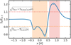 |
Fig. 2 Definition of the widths of the dust ring and gap. The red and yellow shaded regions show the numerically calculated widths of the dust ring and gap. The circles mark Σd,max and Σd,min. |
2.5.4 Definition of the depth of the dust gap
We defined the dust gap depth as the contrast between the minimum and maximum dust surface densities (Fig. 2; Huang et al. 2018; Zhang et al. 2018). We numerically calculated the dust gap depth as
 (18)
(18)
It should be noted that Eq. (18) may represent the amplitude of the dust ring if turbulent diffusion smooths the dust gap and then only the dust ring forms. Although it can differ from the intuitive definition of the dust gap depth, we consistently use Eq. (18) for measuring the dust gap depth.
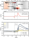 |
Fig. 3 Perturbation of the planet-induced gas flow on the radial velocity of dust and the dust surface density. We set m = 0.1, ℳhw = 0.03, St = 10−3, and αdiff = 10−4. Top: gas flow structure at the meridian plane. The color contour represents the gas velocity in the x-direction averaged in the y-direction within the calculation domain of hydrodynamical simulation, 〈vx,g〉y. The vertical dotted lines represent the x-coordinates of the edges of the outflow region, |

3 Numerical results: time evolution of Σd(t)
In this section we present the numerical results of this study, comparing them with the steady-state solutions Paper (I). We describe the physical processes of the time evolution of the dust surface density. Based on the results presented in this section, we introduce the semi-analytic models of the widths of the dust ring and gap and the depth of the dust gap in Sect. 4.4.
We describe the behavior of the time evolution of Σd(t) influenced by the planet-induced gas flow. Given the wide parameter spaces in our study, we first show the numerical results for a fiducial parameter set with αdiff = 10−4, m = 0.1, ℳhw = 0.03, and St = 10−3 (Sect. 3.1). We then show the dependence of Σd(t) on the turbulent parameter (Sect. 3.2), the planetary mass (Sect. 3.3), the Mach number of the headwind (Sect. 3.4), and the Stokes number (Sect. 3.5), respectively.
3.1 Fiducial case
The outflow of the gas at the midplane induced by low-mass planets perturbs the radial drift velocity of dust, causing the dust rings and gaps (Fig. 3). Figure 3 shows the perturbations of low- mass planets on the gas and dust, where we set αdiff = 10−4, m = 0.1, ℳhw = 0.03, and St = 10−3, as the fiducial parameter set. In Fig. 3, the top, the middle, and the bottom panels show the velocity field of the gas at the meridian plane, the radial drift velocity of dust influenced by the gas flow, and the dust surface density, respectively.
The dust surface density, which has initially a flat profile, changes with time, and then reaches a steady state within t ≲ 106 (Fig. 3). The outflow of the gas at the midplane perturbs the radial drift velocity of dust, causing positive and negative peaks in the profile of 〈vd〉 (the middle panel of Fig. 3). The radially- outward (inward) outflow of the gas inhibits (enhances) the radial drift of dust. The dust surface density decreases with time around the planetary orbit creating a dust gap, while it increases with time outside the planetary orbit creating a dust ring. The dust surface density only changes by a factor of ∼2 in Fig. 3 due to efficient dust diffusion. Given a characteristic length of a perturbation is set by ℒ = 𝒲out, the drift and diffusion timescales are given by tdrift ~ 1.2 × 10⁴ and tdrift ~ 5.2 × 10³, resulting in a diffusion-dominated regime tdiff < tdrift.
The locations of the edges of the dust gap are determined by those of the edges of the outflow region,  (Eq. (10); the vertical dotted lines in Fig. 3). Thus, the dust gap widths can be estimated by 𝒲out (Eq. (12)). The location of the inner edge of the dust ring is set by
  and hardly changes with time. The outer edge of the dust ring moves with time due to diffusion (Fig. 3).
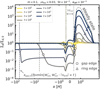 |
Fig. 4 Time evolution of the dust surface density in low-turbulence disks. We set m = 0.1, ℳhw = 0.03, St = 10−3, and αdiff = 10−5. The horizontal axis is on a log scale, whose range is extended to x ∈ [−100, 5]. The vertical dashed lines show the analytic model of the location of the inner edge of the dust gap, which moves with vdrift (Sect. 4.4). |
3.2 Dependence of Σd (t) on the turbulent parameter
A perturbation to Σd (t) due to the planet-induced gas flow strongly depends on the turbulent parameter. Figure 4 shows the time-dependent Σd(t) in the low-turbulence disk (αdiff = 10−5). The planetary mass, the Mach number of the headwind, and the Stokes number are the same as in the fiducial case. Compared to the fiducial case, Σd (t) changes more significantly, because a steep gradient of Σd needs to achieve a steady state due to inefficient dust diffusion (tdiff > tdrift in Fig. 4). In Fig. 4, Σd(t) increases (decreases) by ∼3–4 orders of magnitude. The dust surface density reaches the steady state after t > 108.
During the time evolution Σd(t) changes in a complex manner. The profile of Σd(t) deviates significantly from the steadystate solution. The dust accumulates over time at  , which is similar to the fiducial case. At
  , the dust surface density drops significantly in the early stage of the time evolution, t ≲ 104–105. Due to inefficient dust diffusion, the dust hardly leak out to the inside of the planetary orbit. As a result, at the early stage of the time evolution, the minimum value of Σd(t) can be orders of magnitude smaller than that of the steady-state solution.
Moreover, we found that the dust gap expands with time, and then the dust is depleted in a wide range of  when m ≳ 0.1 (Fig. 4; see also Fig. C.1 for different planetary masses; available on Zenodo3). We found that the inner edge of the dust gap moves with |vdrift|. In this case, the dust gap width can no longer estimated by 𝒲out (Eq. (12)). Because we assumed a constant supply of dust from the outer region of the disk, the dust slowly leaks to the inside of the planetary orbit, and then Σd (t) at
  increased in the late stage of the time evolution, t ≳ 108.
For illustrative purposes, we also display these time sequences in a two-dimensional (2D) plane in Fig. 5, which were generated from the results of 1D calculations shown in Fig. 4. The dust cavity, the gap as wide as the planet’s orbital distance, forms after t ≥ 106 . The cavity-opening timescale can be estimated by Eq. (7) with ℒ = rp. We note that our model for the dust surface density evolution ignores the effect of curvature (Eq. (5)).
A disk with a dust cavity formed by the gas-flow mechanism could be observed as a transition disk (Francis & van der Marel 2020), although the dependence of the cavity evolution time on m, ℳhw, St, and αdiff remains unclear. We speculate that the dust cavity is filled on long timescale (≳106–107 , corresponding to > 5–50 Myr at 10 au; Fig. 6). Since the cavity is filled by diffusion of dust at the ring, we considered that the cavity-filling timescale would be proportional to the formation timescale of the dust ring (Eq. (35) of Paper I): τcav,fill ~ Mring/Ṁdust, where Mring is the mass of the steady-state dust ring and Ṁdust is the radial inward mass flux of dust. We discuss the implications for transition disks in Sect. 5.3.1.
 |
Fig. 5 Time evolution of Σd(t) in the two-dimensional plane. We set m = 0.1, ℳhw = 0.03, St = 10−3, and αdiff = 10−5. These images were generated based on the results of 1D calculations assuming an axisymmetric dust distribution, neglecting disk curvature. The axes are normalized by the planet location, rp, calculated by X = Y = (r − rp)/hp, where r is the radial coordinate centered at the star and hp is the disk aspect ratio at r = rp. We set hp = 0.05. |
3.3 Dependence of Σd (t) on the planetary mass
When higher-mass planets are assumed, we find deeper dust gaps and higher concentrations of dust in a ring. In Fig. 7, the Mach number of the headwind, the Stokes number, and the turbulent parameter are the same as in the fiducial case: ℳhw = 0.03, St = 10−3, and αdiff = 10−4. The location of the outer edge of the dust gap,  , hardly changes when m ≳ 0.3, at which point
  converges (Eq. (10)). The dust gap depths converge at m ≳ 0.3. This is because the outflow speed in the x-direction has a peak at m ~ 0.3 and then the influence of the gas flow on the dust motion saturates (Kuwahara & Kurokawa 2024). In Paper I, where we only considered m = 0.03, 0.1, and 0.3, we set the condition of the dust ring and gap formation as m ≳ 0.1. However, we found that even low-mass planets with m = 0.05 can generate dust rings and (or) gaps (zoom-in panels of Fig. 7, see also Fig. C.1 for αdiff = 10−5).
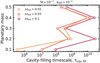 |
Fig. 6 Cavity-filling timescale. We only focus on m ≥ 0.1 in which the dust cavities form. |
3.4 Dependence of Σd (t) on the Mach number of the headwind
The amplitude of the dust ring becomes higher when the larger ℳhw is assumed (Fig. 8). The flow speed of the radially-outward outflow increases with ℳhw (Kuwahara & Kurokawa 2024), which leads to higher concentrations of dust into a ring outside the planetary orbit.
3.5 Dependence of Σd (t) on the Stokes number
In this section we focus on the dependence of Σd(t) on the Stokes number. In Fig. 9, the planetary mass, the Mach number of the headwind, and the turbulent parameter are the same as in the fiducial case: m = 0.1, ℳhw = 0.03, and αdiff = 10−4.
Paper I found that the deeper dust gaps and higher concentrations of dust into a ring can be seen for the smaller Stokes numbers in a steady state, because smaller dust particles are more sensitive to the gas flow. This is successfully reproduced in Fig. 9d. The time required to reach the steady state is shorter when the larger Stokes number is assumed (Figs. 9a–c, see also Fig. C.2 for αdiff = 10−5), because the drift timescale of dust is shorter for the larger Stokes numbers (tdrift ∝ St−1 ; Eq. (7)).
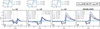 |
Fig. 7 Dependence of Σd(t) on the planetary mass. We set ℳhw = 0.03, St = 10−3, and αdiff = 10−5. The vertical dotted lines correspond to |x| = 4/3 (the x-coordinate of the edge of the outflow region for m ≳ 0.3; Eq. (12)). The small panels above the upper left corners of panels a-c are the zoomed-in views for m = 0.03, 0.05, and 0.07. |
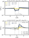 |
Fig. 8 Dependence of Σd(t) on the Mach number of the headwind. We set m = 0.2, St = 10−3, and αdiff = 10−4. We varied the Mach number of the headwind in each panel, ℳhw = 0.01 (top) and ℳhw = 0.1 (bottom). |
3.6 Summary of the parameter dependence
We summarize the dependence of Σd(t) on αdiff, m and St for a fixed ℳhw and the time in Fig. 10. We set ℳhw = 0.03 and t = 105 in Fig. 10. A perturbation to Σd(t) is stronger when the smaller αdiff, the higher-mass planets, or the smaller St are assumed.
Figure 11 is a contour plot of the dust gap depth as a function of the planetary mass and the Stokes number for a fixed ℳhw and time (ℳhw = 0.03 and t = 105), showing that the dust gap forms when m ≳ 0.05 and the dust gap deepens as the planetary mass increases. At t = 105, the dust gap depth has a peak at St = 10−3.
4 Properties of dust rings and gaps
This section shows the widths of the ring and gap and depth of the gap. We first show the numerical results in Sects. 4.1–4.3. We then introduce semi-analytic models of dust rings and gaps in Sect. 4.4 based on the obtained numerical results.
4.1 Numerically calculated dust gap width
We found that the dust gap width either stays constant or expands with time (Fig. 12). In general, once the dust gaps form, their widths do not change significantly with time in the moderateturbulence disks (αdiff = 10−4; Fig. 12a), because Σd(t) decreases only within the outflow region (Fig. 3). The dust gap widths increase with the planetary mass when m ≲ 0.3, and converge at m ≳ 0.3. These numerical results can be explained by the dependence of 𝒲out on the planetary mass, which is independent of time. It increases with the planetary mass when m ≲ 0.3, and has a constant value at m ≳ 0.3 (Fig. 1).
The dust gap keeps expanding with time when m ≳ 0.1 after t ≳ 104 in the low-turbulence disk (αdiff = 10−5; Fig. 12b). Since the inner edge of the dust gap moves with |vdrift| (Fig. 4), the width of the expanding dust gap is independent of the planetary mass. We note that the semi-analytic model of the dust gap width (the dashed lines in Fig. 12) will be introduced in Sect. 4.4.
4.2 Numerically calculated dust gap depth
The dust gaps deepen initially with time, and then their depths  converge after t ≳ 103–104 (Fig. 13). Initially,
  decreases because the dust surface density decreases at
  . As Σd(t) stops decreasing at
  or a decrease in Σd(t) at
  balances an increase in Σd(t) at
  after t ≳ 103–104, the dust gap depth eventually becomes constant (Fig. 4). The dust gaps deepen with the planetary mass when m ≲ 0.3 and their depths converge at m ≳ 0.3 (Fig. 14), because the outflow speed has a peak at m ∼ 0.3 and, consequently, the perturbation of the gas flow on the dust motion saturates (Kuwahara & Kurokawa 2024). We note that the semi-analytic model of the dust gap depth (the dashed lines in Fig. 13) will be introduced in Sect. 4.4.
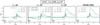 |
Fig. 9 Dependence of Σd(t) on the Stokes number. We set m = 0.1, ℳhw = 0.03, and αdiff = 10–5. The vertical dotted lines correspond to |

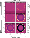 |
Fig. 10 Summary of the parameter dependence of Σd(t). We set ℳhw = 0.03 and t = 105. We varied the planetary mass, the Stokes number, and the turbulent parameter. |
4.3 Numerically calculated dust ring width
The dust ring widths increase with time due to diffusion and then reach a steady state (Fig. 15). The dust ring widths have the radial extent of ≲1–10 times the gas scale height, which is weakly dependent on the planetary mass. Figure 15 summarizes the parameter dependence of the dust ring width at a certain time, showing the following trends. (1) The dust ring width decreases as St increases (Figs. 15a and b). (2) The dust ring width increases as αdiff increases (Figs. 15b and c). (3) The dust ring width decreases as ℳhw increases (Figs. 15c and d). These trends suggest that the dust ring width is proportional to the length where the drift timescale coincides with the diffusion timescale:  . We note that the semi-analytic model of the dust ring width (the dashed lines in Fig. 15) will be introduced in Sect. 4.4.
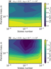 |
Fig. 11 Contour plot of the dust gap depth as a function of the planetary mass and the Stokes number. We set ℳhw = 0.03 and t = 105. We varied the turbulent parameter in each panel, αdiff = 10–4 (panel a) and αdiff = 10–5 (panel b). |
4.4 Semi-analytic models of dust rings and gaps
Based on the obtained numerical results in Sect. 3, we introduce semi-analytic models of the width of the dust ring and gap and the depth of the dust gap as functions of m, ℳhw, St, αdiff, and t. Since a significant perturbation to Σd(t) due to the planet- induced gas flow appears only when the smaller Stokes numbers were assumed, we restrict our attention to the limited range of the Stokes number, St ≲ 10–3.
Section 4.4.1 introduces the semi-analytic model of the dust gap width. By fitting of the numerical results, we derived a criterion for the dust gap width which distinguish between the temporally constant and expanding gaps, and then described the dust gap widths in each case. In Sect. 4.4.2, we considered that the time evolution of the dust gap depth is described by a logistic differential equation. Using an analytical solution to the logistic equation combined with the fitting of numerical results, we obtained the semi-analytic model of the dust gap depth. In Sect. 4.4.3, we considered the time evolution of the dust ring width is described by a sigmoid curve with a steady-state dust ring width as an asymptote. By fitting the sigmoid curve to the numerical results, we obtained the semi-analytic model of the dust ring width.
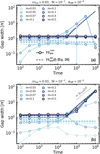 |
Fig. 12 Time evolution of the dust gap width for different planetary masses. We fixed the Stokes number St = 10–3 and the Mach number ℳhw = 0.03, and set αdiff = 10–4 in panel a and αdiff = 10–5 in panel b. The solid lines with the circle symbols and the dashed lines are the numerically calculated and the semi-analytic dust gap widths, respectively (Eq. (26); Sect. 4.4). We note that in panels a and b, the numerically calculated dust gap width for m = 0.03 is not shown because we obtained |

4.4.1 Dust gap width
As mentioned in Sect. 4.1, the dust gap is either constant or expanding with time. The temporally constant dust gap width can be modeled by the width of the outflow region, Wout (Eq. (12)). When the dust gap expands with time, the inner edge of the dust gap is set by  , whichever smaller (Fig. 4).
Considering the dust surface density within the outflow region, we construct a semi-analytic model for the dust gap width,  . We expect that the dust gap width keeps constant,
  , when the diffusive flux of dust dominates the time evolution of the dust surface density, while we assume that the dust gap expands with time when the advective flux dominates. We determine the diffusion-dominated or advection- dominated regime by comparing Σd(x, t) at the gap location with a certain critical value, Σcrit. Given the balance between the advective and diffusive flux of dust, we derive the critical dust surface density:
 (19)
(19)
Here we focus on the limited region,  , in which the radial drift velocity of dust is approximately given by ⟨vd⟩ ∼ vdfrit (the middle panel of Fig. 3). We set ⟨vd⟩ = vdrift for simplicity in Eq. (19). We then integrate Eq. (19) over a range of
 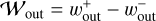 (Eq. (12)) and obtain
 (20)
(20)
Equation (20) gives
![${\Sigma _{\rm{d}}}\left( {w_{{\rm{out}}}^ + } \right) = {\Sigma _{{\rm{d}},0}}\exp \left[ { - {{2{\rm{St}}{{\cal M}_{_{{\rm{hw}}}}}{{\cal W}_{_{{\rm{out}}}}}} \over {{\alpha _{{\rm{diff}}}}}}} \right] \equiv {\Sigma _{{\rm{crit}}}},$](/articles/aa/full_html/2024/12/aa51159-24/aa51159-24-eq49.png) (21)
(21)
where we set  and assume 1 + St2 ≃ 1. The diffusive (advective) flux of dust dominates the time evolution of the dust gap when Σd(x, t) > ∑crit (Σd(x, t) < ∑crit) within the limited region,
  . We compared the time evolution of the dust surface density with Σcrit in Fig. A.2.
Practically, we consider that the dust gap stays constant when  and expands with time when
  , where
  is the global minimum of the time-dependent dust surface density at the gap location:
 (22)
(22)
We find that  can be fitted by (Appendix B)
 (23)
(23)


with erf being the error function (erf(m) → 1 when m → ∞).
In summary, the semi-analytic formula of the dust gap width is given by
 (26)
(26)
We plotted Eq. (26) in Fig. 12 with the dashed line (see also Fig. C.3). In Fig. 12, Eq. (26) predicts that the dust gaps keep expanding with time when m ≳ 0.1–0.2 at t ≳ 104, which is consistent with the numerical results in the low-turbulence disk (αdiff = 10–5; Fig. 12b). When αdiff = 10–4, Eq. (26) fails to reproduce the numerical results for m ≥ 0.2 which are constant with time (Fig. 12a). We speculate that this deviation is caused by the assumption of ⟨vd⟩ ∼ vdfrit in Eq. (19). Nevertheless, we use Eq. (19) as it reproduces an overall trend in the planetary-mass dependence.
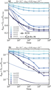 |
Fig. 13 Time evolution of the dust gap depth for different planetary masses. We fixed the Stokes number St = 10–3 and the Mach number ℳhw = 0.03, and set αdiff = 10–4 in panel a and αdiff = 10–5 in panel b. The solid lines with the circle symbols and the dashed lines are the numerically calculated and the semi-analytic dust gap depths, respectively (Eq. (28); Sect. 4.4). |
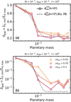 |
Fig. 14 Dust gap depth as a function of planetary mass at t = 106. We fixed the Stokes number St = 10–3 and set αdiff = 10–4 in panel a and αdiff = 10–5 in panel b. The solid lines with the circle symbols and the dashed lines are the numerically calculated and the semi-analytic dust gap depths, respectively (Eq. (28); Sect. 4.4). |
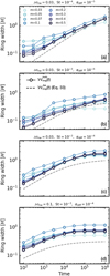 |
Fig. 15 Time evolution of the dust ring width for different planetary masses. The assumed parameters (ℳhw, St, and αdiff) are shown at the top of each panel. The solid lines with the circle symbols and the dashed lines are the numerically calculated and the semi-analytic dust ring widths, respectively (Eq. (33); Sect. 4.4). |
4.4.2 Dust gap depth
As described in Sect. 4.2, the dust gap depth deepens with time and has a lower limit. We assume that the time evolution of the dust gap depth obeys the following equation4:
![$\delta _{{\rm{gap}}}^{SA}(t) = {\delta _\infty }{\left[ {1 - \left( {1 - {{{\delta _\infty }} \over {{\delta _0}}}} \right){e^{ - t/{\tau _{{\rm{gap}}}}}}} \right]^{ - 1}},$](/articles/aa/full_html/2024/12/aa51159-24/aa51159-24-eq61.png) (28)
(28)
where  is the semi-analytic model of the dust gap depth, δ∞ is the steady-state dust gap depth,
  , and τgap is the characteristic timescale. Equation (28) shows that
  decreases with time and then approaches the steady-state value,
  , at t >> τgap. We define
 (29)
(29)
where we set ℒ = 0.41 × Wout in both tdrift and tdiff (Eqs. (7) and (8)). The coefficient of 0.41 is determined by the least-squares fitting of numerical results. The characteristic timescale τgap is a function of m, ℳhw, St, and αdiff, having on the order of ~ 103 –104 in our parameter sets.
We find that the steady-state dust gap depth can be fitted by (Appendix B)
 (30)
(30)


We plotted Eq. (28) in Figs. 13 and 14 (see also Fig. C.4) with the dashed line. Although Eq. (28) does not completely reproduce the numerical results, it shows good agreement with the numerical result, in particular when t ≳ τgap ∼ 103–104. When t ≲ τgap , Eq. (28) only agrees with the numerical results of m < 0.1. We speculate that the deviation is caused by the assumption of τgap , which is set by the drift or the diffusion timescale with ℒ ∝ Wout, whichever smaller (Eq. (29)). However, the radial drift speed of dust deviates from the unperturbed value within the outflow region, which changes tdrift.
4.4.3 Dust ring width
As described in Sect. 4.3, the dust ring width increases with time and then reaches a steady state. We assume that the time evolution of the dust ring width is described by the following sigmoid curve:
 (33)
(33)
Here  is the semi-analytic model of the dust ring width,
  is the fitting formula for the steady-state dust ring width, τring is the characteristic timescale, and q = 0.42 (Appendix B). Numerical results showed that
  would be proportional to Leq (Eq. (9)), and, consequently, αdiff (Sect. 4.3), but we find that the dependence is weaker than
  . We find that
  can be fitted by (Appendix B):
 (34)
(34)
The dust rings expand due to dust diffusion. Thus, we define
 (35)
(35)
We plotted Eq. (33) in Fig. 15 (see also Fig. C.5) with the dotted lines, which show good agreement with the numerical results.
4.4.4 Caveat
So far we have considered the regime in which the dust is tightly coupled with the gas, St ≲ 10–3. Since we developed our semi-analytic models by fitting the numerical results with St = 10–3 (Appendix B), our semi-analytic models would be invalid when St ≳ 10–2. Figure 16 compares our semi-analytic model for the dust gap depth with the numerical result when St = 10–2, showing a significant deviation appears in particular when αdiff = 10–5.
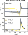 |
Fig. 17 Time-dependent dust surface density with particle sizes of s = 3.7 mm perturbed by an Earth-like planet (Mp = 0.66M⊕) at 1 au. Numerical simulations were conducted in dimensionless units. We set m = 0.1, ℳhw = 0.03, St = 10–3, and varied the turbulent parameter in each panel, αdiff = 10–5 (panel a) and αdiff = 10–4 (panel b). For the assumed parameter set, the pebble isolation masses are given by Miso = 2.8 M⊗ (panel a) and 3 M⊗ (panel b; Eq. (A.14)). |
5 Discussion
5.1 Time evolution of Σd (t) with dimensional units
To facilitate the interpretation of our results, we rewrite our numerical results with dimensional units. Assuming that a typical steady accretion disk model (Ida et al. 2016), we convert the dimensionless quantities into the dimensional ones. Appendix A describes the method for the conversion. We set the orbital radius of the planet as rp = 1 au or 50 au, at which the Mach number of the headwind has the value of ℳhw = 0.03 or 0.1 (Eq. (A.10)).
Here we show the time-dependent dust surface density Σd(t) with sizes of s ≈ 4 mm-sized particles (St = 10–3) perturbed by gas flow induced by an Earth-like planet at 1 au (Sect. 5.1.1). We also show solids with sizes of s ≈ 0.2 mm (St = 3 × 10⁻³) perturbed by a Neptune-like planet at 50 au (Sect. 5.1.2). The dust size was chosen to be consistent with nonsticky slicate grains inside the H2O snow (≲ a few au) and with nonsticky icy CO2- covered grains outside the CO2 snow line located approximately outside 10 au (Musiolik et al. 2016a,b). This limits particle sizes to ~2 mm at ~1 au and ~0.4 mm at 50 au (Okuzumi & Tazaki 2019).
5.1.1 Earth-like planet at 1 au
Figure 17 shows the evolution of the solid surface density Σd(t) of ~4 mm sized particles around an Earth-like planet with a mass of ~0.7 M⊗ embedded at 1 au in a disk with low midplane turbulence (αdiff = 10–5; Fig. 17a) and in a disk with moderater midplane turbulence (αdiff = 10–4; Fig. 17b). In the low-turbulence disk, the dust is depleted by ~2 orders of magnitude within 1 Myr at <1 au (Fig. 17b). A significant amount of dust concentrates into a very narrow ring whose width is less than 0.1 au at the planet location. In the narrow ring, Σd (t) increases by ~102 times the initial value. In contrast, in the moderate-turbulence disk (αdiff = 10–4; Fig. 17a), the Earthmass planets do not create a significant dust depletion nor concentration for the assumed parameters. A shallow dust gap appears within 0.1 Myr at <1 au, but it is smoothed within 1 Myr. Only a narrow dust ring whose width is ~ 0.1 au remains outside the planet location at 1 Myr.
The assumed planetary mass (Mp ≃ 0.7 M⊗) falls below the pebble isolation mass (Miso ≈ 3 M⊗; Lambrechts et al. 2014; Bitsch et al. 2018) at which a growing planet opens a shallow gas gap and then the pebble flux is highly reduced inside the planetary orbit. Even planets with masses below the pebble isolation mass can affect significantly Σd(t). When the planetary mass exceeds m ≳ 0.1 (Mp ≳ 0.7 M⊗ at 1 au), the subsequent growth of the planet would be suppressed and planets remain small in the terrestrial planet forming-region.
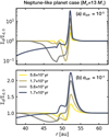 |
Fig. 18 Time-dependent dust surface density with particle sizes of s = 0.23 mm for a Neptune-like planet (Mp = 13 M⊗) at 50 au. The numerical simulations were conducted in dimensionless units. We set m = 0.1, ℳhw = 0.1, St = 3 × 10⁻³, and varied the turbulent parameter in each panel, αdiff = 10–5 (panel a) and αdiff = 10–4 (panel b). For the assumed parameter set, the pebble isolation masses are given by Miso = 56 M⊗ (panel a) and 60 Mæ (panel b; Eq. (A.14)). |
5.1.2 Neptune-like planet at 50 au
Figure 18 shows a situation where a Neptune-like planet, ~13 M⊗, is located at 50 au. In both the low- and moderate-turbulence disks (αdiff = 10−5 and 10−4), the Neptunelike planet can generate the dust ring and gap whose widths are a few au in the distribution of ~ 0.2 mm sized dust within 1 Myr.
5.2 Implications for planet formation via pebble accretion
Once the gap forms in the distribution of pebbles, it reduces the accretion rate of pebbles onto protoplanets. As shown in Fig. 17a, even planets with masses below the pebble isolation mass can affect significantly Σd(t). When the planetary mass exceeds m ≳ 0.1 (Mp ≳ 0.7 M⊕ at 1 au), the subsequent growth of the planet would be suppressed and planets remain small in the terrestrial planet forming-region. The suppression of pebble accretion in the terrestrial planet forming-region due to the dust-gap-opening effect by the gas-flow mechanism may be helpful in explaining the current observed period-mass diagram of exo-planets, in which a large fraction of low-mass planets (≲10 M⊕) has been found at short-period orbits (≲100 days; e.g., Fressin et al. 2013; Weiss & Marcy 2014, see Sect. 4.4.2 of Paper I for further discussion).
5.3 Comparison to disk observations
We compared our semi-analytic models of the widths of the dust ring and gap with the observational data, finding that a fraction of the observed dust rings and gaps could be explained by the gas-flow driven by low-mass planets. We considered here a single planet embedded in a disk. Provided that the thermal emission of the dust is optically thin, and the opacity and the temperature are constant within a dust substructure, the dust surface density is proportional to the observed intensity profile, Σd ∝ Iv. In the following paragraphs, we only compared our semi-analytic models with the observed widths of the dust ring and gap. A direct comparison of our semi-analytic model of the dust gap depth with the observational data is difficult because the optically thin assumption would be invalid at the dust ring locations (Guerra-Alvarado et al. 2024; Ribas et al. 2024) and, consequently, the observed intensity does not correspond to a unique dust surface density. In the highly optically thick regime the rings may not be observed, because strong optical depth effects lead to flat-topped radial intensity profiles (Dullemond et al. 2018). Our semi-analytic model of the dust ring width is valid as long as a ring with a moderate optical depth is detectable in the radial intensity profile. The uncertainty in the optical depth of the observed no-flat-topped ring does not significantly affect the observed value of the dust ring width (Dullemond et al. 2018).
To compare with the observational data, we converted the units of  and
and  from H to au using Eq. (A.3). Same as in Sect. 5.1, we considered the typical steady accretion disk model with the fixed stellar mass, stellar luminosity, and the mass accretion rate (Appendix A): M* = 1 M⊙, L* = 1 L⊙, and Ṁ* = 10−8 M⊙/yr. We note that rings and gaps have been observed around various types of stars, so that, in reality, these values vary in disks (Huang et al. 2018; Long et al. 2018; Bae et al. 2023): M* ~ 0.2–2 M⊙, L* ~ 0.1–20 L⊙, and Ṁ* ~ 10−10–10−7 M⊙/yr.
5.3.1 Dust gap width
Figure 19 compares our semi-analytic model of the dust gap width,  , with the observational data,
  , in which the dust gap widths are plotted as a function of the gap location, rgap. The observational data were obtained from the Atacama Large Millimeter/submillimeter Array (ALMA) surveys (Huang et al. 2018; Long et al. 2018; Zhang et al. 2023), including the Disk Substructures at High Angular Resolution Project (DSHARP; Huang et al. 2018). The assumed Stokes number and the Mach number of the headwind to plot
  were the same values as in the fiducial case: St = 10−3, and ℳhw = 0.03.
About 20% of the observed dust gaps, whose widths are comparable to the gas scale height  , could be explained by our gas-flow mechanism in the moderate-turbulence disks (αdiff = 10−4; Fig. 19a). The gas-flow mechanism has the potential to explain the observed wide dust gaps with
  by assuming weaker midplane turbulence (αdiff = 10−5) and a long time evolution exceeding t ≳ 104. Given that an upper limit for the time required for gap formation is 3 Myr, ~65% of the observed gaps can be explained (Fig. 19b).
These comparisons may suggest the existence of low-mass planets (m ≳ 0.05) at wide orbits as an origin of the observed dust gaps, which could be consistent with a large population of such planets inferred from a population synthesis model (Drazkowska et al. 2023). However, it is difficult to constrain the masses of unseen planets, because the dust gap widths in our model converge when m ≳ 0.3 or t ≳ 104 (Fig. 12).
Figure 19 suggests that low-mass planets within ≲ 10 au could carve gaps as wide as their location, which are entering the transition disk regime (Francis & van der Marel 2020). However, since the dependence of the evolution time of the dust cavities on the parameters (m, ℳhw, St, and αdiff) is unclear (Fig. 6), further investigations are needed to link the transition disks with our gas-flow mechanism.
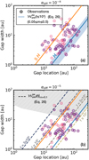 |
Fig. 19 Dust gap width as a function of the dust gap location. We set St = 10−3 and ℳhw = 0.03, and varied the turbulent parameter in each panel, αdiff = 10−4 (panel a) and αdiff = 10−5 (panel b). The blue and orange solid lines denote H and 5 H, respectively (Eq. (A.3)). Panel a: Blue shaded region given by |

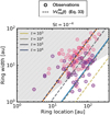 |
Fig. 20 Dust ring width as a function of the ring location. We set ℳhw = 0.03 and αdiff = 10−4. The dashed and dotted lines are given by Eq. (33) with St = 10−3 and 10−4, where we converted the units of |

5.3.2 Dust ring width
The observed dust ring widths range from a few au to a few tens of au, which are predominantly wider than those predicted by our semi-analytic model. Figure 20 compares our semi-analytic model of the dust ring width with the observational data,  , in which the dust ring widths are plotted as a function of the ring locations. The observational data were compiled from Huang et al. (2018) and Bae et al. (2023). The assumed Mach number of the headwind and the turbulent parameter to plot
  were the same values as in the fiducial case: ℳhw = 0.03 and αdiff = 10−4. We considered St = 10−4 in Fig. 20. We note that we do not show αdiff = 10−5 or St = 10−3 because it leads to narrower gaps and poor agreement with observed rings.
About 15% of the observed rings, whose widths are less than  , could be explained by the gas-flow mechanism, given that an upper limit of the time required for ring formation is 3 Myr (Fig. 20). We found that only ~3% of the observed dust rings could be explained by the gas-flow mechanism when St = 10−3 and αdiff = 10−4. This may suggest that the dust particles at rings are small due to collisional fragmentation or bouncing (Blum & Wurm 2008; Güttler et al. 2010; Zsom et al. 2010). The inferred Stokes numbers at the dust rings in this study are consistent with the results of dust growth simulations considering the fragility of porous dust (St ~ 10−4–10−3; Ueda et al. 2024). However, when compact dust was considered, larger Stokes numbers were inferred from the multi-wavelength analysis of the continuum emission, the modeling of dust rings at gas pressure maxima, and the dust growth simulations (St ~ 10−3–10−1; Sierra et al. 2021; Doi & Kataoka 2023; Jiang et al. 2024). Further discussion is difficult, because the observed wide rings might not sufficiently resolved, and thus they could be composed of multiple narrow rings (Bae et al. 2023).
5.3.3 Potential of multiple planets
So far we have been only considered the dust ring and gap formation by a single planet. The observed wide dust gaps with  may also be explained by the radially-outward gas flows induced by the multiple planets. When the multiple planets are embedded in the disks with an orbital separation of
  , the wide dust gaps may form which are shared by the multiple planets, although the orbital stability of planets is beyond the scope of this study. In this case, a single dust ring forms outside the orbit of the outermost planet.
The observed wide rings may consist of the narrow rings. When the multiple planets are embedded in the disks with the orbital separation of  , the multiple rings may form with a separation of ~∆a. If the spatial resolution of the observations is low (≳ H), these multiple narrow rings may be observed as a single wide ring.
5.4 Implications for future disk observations
The relatively deep and wide dust gaps formed by the gas flows driven by low-mass planets in the process of their formation in the inner few au of low-turbulence disks could be detected by future observations (Fig. 17a). Due to limitations of the angular resolution, it is difficult to detect the dust substructures in the inner few au of disks by current observations. A possible future extension would improve the angular resolution of the current ALMA by several times, which could lead to further detection of dust substructure in the inner few au of disks (Carpenter et al. 2020; Burrill et al. 2022). A next-generation Very Large Array (ngVLA) is expected to capture the dust thermal emission at ~mm–cm wavelengths with the best angular resolution of ~0.001 arcsec (Selina et al. 2018), which will also provide the capability to probe the inner few au of disks. Simulations of ngVLA observations suggest that the dust gaps with the widths of ~2–3 au are detectable at ~5 au under weak turbulence (αdiff ≲ 10−5; Ricci et al. 2018; Harter et al. 2020).
Future high angular resolution observations may also detect narrow dust rings and gaps with widths comparable to or less than the gas scale height, H. Thus, our gas-flow mechanism needs to be compared with these future observations.
Future observations may detect the outflow region produced by our gas-flow mechanism. The spatial scale of the outflow region is on the order of the disk gas scale height, ~ H ≈ 8.9 au(r/100au)9/7 (Eq. (A.4)), in the radial and azimuthal directions (Kuwahara & Kurokawa 2024). The maximum amplitude of the velocity perturbation of the outflow is ~0.3 cs = 0.03 υK(h/0.1)≃0.09km/s(r/100au)−1/2(M*/M⊙)1/2 (Kuwahara & Kurokawa 2024). Given that the distance to the disk is 100 parsecs and a planet is embedded in the disk at 100 au, the capability to resolve the disk at ~ 0.1 arcsec and ~ 0.1 km/s is required. The current ALMA has the angular resolution of ≳ 0.1 arcsec and the velocity resolution of ≳ 0.01 km/s for the gas. The kinematic features of the outflow induced by low-mass planets may be detectable. However, as discussed in Sect. 4.5.2 of Paper I, the kinematic features of the outflow can only be appeared in the region close to the midplane (ɀ < H; Fig. 3). Therefore, molecules that can trace low heights in disks, such as C17O, HCN, and C2H, should be used as tracers.
5.5 Comparison to previous studies
Previous studies have mostly focused on gap-opening planets to explain the observed dust gap widths (the gas-gap mechanism), often using empirical relations between the planetary mass and the dust gap width obtained from the disk-planet interaction simulations. Zhang et al. (2018) performed 2D hydrodynamical simulations of gas and dust with gas-gap-opening planets. The authors defined the dust gap width by ∆Z18 ≡ (rout – rin)/rout, where rin and rout are the edges of the dust gap normalized by the planet location rp, and then obtained ∆Z18 ~ 0.1–1 for different disk models with h = 0.05, 0.07, and 0.1. In our dimensionless unit, the dust gap width defined in Zhang et al. (2018) can be described by 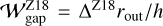 . Assuming rout ~ rp ≡ 1, we obtained
  .
.
An empirical relation in which the dust gap width is assumed to be proportional to the Hill radius has been obtained by the hydrodynamical simulations with gas-gap-opening planets ( ; Rosotti et al. 2016; Lodato et al. 2019; Wang et al. 2021). In our parameter sets, the Hill radius ranges from RHill ≃ 0.22 to 0.55, which leads to
  .
.
Dong et al. (2018) performed 2D hydrodynamical simulations of gas and dust with embedded planets, investigating the dust gap formation due to the shallow gas-gap opening by a planet under the weak turbulence condition (αdiff ≲ 10). The authors considered the planets with m = 0.04–0.8, obtaining the empirical relations between the dust gap width and the planetary mass,  , where lsh is the so-called shocking length of the density waves launched by an embedded planet (Goodman & Rafikov 2001):
 (36)
(36)
Here γ = 1.4 is the adiabatic index. Thus, in our dimensionless unit, we obtained  .
.
The dust gap widths obtained in this study are narrower than those obtained in the previous studies mentioned above as long as a temporally constant dust gap was considered,  . The difference in dust gap widths obtained in the previous studies and this study is attributed to different physics and the different parameter range of the Stokes number assumed in each study. The models for dust ring and gap formation driven by higher-mass planets carving gas gaps (the gas-gap mechanisms) are more susceptible to occur when larger Stokes numbers are assumed (St ≳ 10−3–10−2; Zhu et al. 2012, 2014; Rosotti et al. 2016; Weber et al. 2018). Then the dust particles are trapped at x ≳ H. On the other hand, our gas-flow mechanism works well for smaller solids with St ≲ 10−2. Such dust particles are trapped by the outflow of the gas at x ≲ 2/3 H.
Although we did not consider the (shallow) gas-gap formation in this study, we would expect that the gas-flow mechanism can coexist with the gas-gap-opening mechanism. The gas-gap mechanism generates the dust gaps with 𝒲gap ≳ H in the distribution of large dust (St ≳ 10−3–10−2). Because the small dust particles can pass through the gas gap due to diffusion or the viscous accretion flow (e.g., Rice et al. 2006), the dust gaps also form in the distribution of small dust (St ≲ 10−2) by the gas-flow mechanism, whose widths depend on the assumed parameters. The locations of the outer edge of the dust gaps should differ between the gas-flow and gas-gap-opening mechanisms.
Several studies have shown that low-mass planets, which do not form gas gaps or pressure bumps, can create rings and gaps. The gravitational torque exerted by embedded planets can carve gaps that appear only in the dust distribution (Muto & Inutsuka 2009; Dipierro & Laibe 2017). Muto & Inutsuka (2009) showed that, when the global pressure gradient of the disk gas is neglected, a planet with a mass of 2 M⊕ can open a gap in the distribution of large dust grains (St ≳ 0.1). Dipierro & Laibe (2017) derived a grain-size-dependent criterion for dust gap opening in disks, showing that a planet with a mass of ≲10 M⊕ can carve a dust gap when St ≳ 1.
Compared to these previous studies that work well for the dust with large Stokes numbers, our results show the opposite trend. In our study, dust rings and gaps form when the smaller Stokes numbers are considered (St ≲ 10−2), as we focused on the potential effect of the gas flow driven by an embedded planet, which was not considered in the previous studies.
5.6 Model limitations
Although we did not consider the evolution of the gas disk, the outer part of a disk evolving with viscous angular momentum transport could spread outward due to the conservation of the angular momentum (Lynden-Bell & Pringle 1974). The disk gas at r > rexp expands outward, where rexp = r0/2(1 + t/tv), r0 is an initial disk radius, and tv is a characteristic viscous timescale at r = r0. The small dust considered in this study could move outward together with the resulting outward flow of the background disk gas (Liu et al. 2022). When a planet is embedded at r > rexp, the dust particles will be trapped by the radially-inward outflow of the gas induced by an embedded planet. Then the dust ring could form inside the planetary orbit and the dust could deplete outside the planetary orbit. However, the direction of the flow of the background disk gas at the midplane is a controversial issue. The disk gas evolution may be driven by magnetic disk winds (e.g., Bai & Stone 2013). The winds extract angular momentum from the disk surface and drive inward gas accretion at the midplane.
Low-mass planets would undergo inward migration (so-called type I migration; Ward 1986; Tanaka et al. 2002). The timescale of the type I migration is described by
 (37)
(37)
where Σg is the gas surface density. The type I migration timescale is comparable or shorter than the timescale for the dust ring and gap formation by the gas-flow mechanism. When the migration timescale is shorter than the timescale for the dust ring and gap formation, the positions of the dust ring and gap do not necessarily coincide with the planet location (Kanagawa et al. 2021).
We fixed the planetary masses in this study, whereas planets grow by pebble accretion. A perturbation to the dust surface density becomes strong as the planetary mass increases. The dust gap widens and deepens as the planetary mass increases if the growth timescale of the planet is shorter than the timescale for the dust gap formation. When the planetary mass exceeds approximately m ~ 0.1–0.3, the gap width is independent of the planetary mass (Fig. 12). Thus, we could constrain the lower bound of the mass of the embedded planet from the observed dust gap width. We also fixed the Stokes number, even though it could be varied by dust growth and fragmentation at the dust rings. These additional processes would further complicate the time evolution of Σd(t) and should be included in further studies.
An eccentricity of an embedded planet could alter our results. A planet on eccentric orbit induces a time-dependent gas flow field (Bailey et al. 2021), in which the radially-outward gas flow would disappear. However, the eccentricity of the planet can be damped by the disk-planet interaction. The eccentricity damping timescale is given by (Tanaka & Ward 2004)
 (38)
(38)
Thus, the dust ring and gap formation by the gas-flow mechanism is valid when the eccentricity damping timescale is shorter than the timescale for the dust ring and gap formation.
We finally note that the backreaction of dust on gas, which is not considered in this study, would be important at the dust rings. When the backreaction is included, the axisymmetric dust rings form without planets due to the self-induced dust trap mechanism (Gonzalez et al. 2017; Vericel & Gonzalez 2020; Vericel et al. 2021). When a planet embedded in a disk, the dust ring outside the planetary orbit with the high local dust-to-gas density ratio (≳1) could be unstable and broken into small-scale dust-gas vortices (Pierens et al. 2019; Yang & Zhu 2020), which could change an axisymmetric morphology of the dust rings considered in this study.
6 Conclusions
We investigated the time evolution of dust rings and gaps formed by low-mass planets inducing a radially-outward gas flow. By fitting our numerical results, we developed semi-analytic models describing the widths of the dust rings and gaps and the depth of the dust gaps. Our main results are as follows:
Under weak turbulence (αdiff ≲ 10−4), low-mass planets with m > 0.05 (corresponding to >0.33 M⊕ at 1 au or ≳1.7 M⊕ at 10 au) can generate dust rings and gaps in the distribution of small dust, St ≲ 10−2.
Dust gaps have a width comparable to the gas scale height, but can expand further in size when m ≳ 0.1 and αdiff ≲ 10−5, at a rate set by the dust drift speed (Eq. (26)).
The dust gap depth deepens as the planetary mass increases when m ≲ 0.3, but converges at m ≳ 0.3 to a depletion factor of δgap ~ 0.2 when αdiff = 10−4 (δgap ~ 10−7 when αdiff = 10−5; Eq. (28)). Deeper dust gaps form when smaller turbulent parameters are assumed.
The dust rings outside of the planetary orbit widen with time due to diffusion and then reach a steady state. The widths range from ~ 0.1 H to 10 H depending on St, αdiff, and ℳhw (Eq. (33)).
By comparing our semi-analytic models of the dust rings and gaps with the observational data, we found that up to approximately 65% (15%) of the observed dust gaps (rings) could be generated by the gas-flow driven by a single low-mass planet. When St = 10−3 and αdiff = 10−4 are considered as the fiducial values, low-mass planets could explain approximately 20% (3%) of the observed dust gaps (rings) with the radial widths of ~ H within t ≤ 104-105, corresponding to ≤ 0.05–0.5 Myr at 10 au. On longer timescales (t ≳ 104–105), the gas-flow mechanism also has the potential to explain approximately 65% (15%) of the observed wide gaps (rings) with widths exceeding the gas scale height H. Wide gaps require a low level of midplane turbulence (αdiff ≲ 10−5) and wide rings require very small Stokes numbers (St ≲ 10−4).
Our model for dust ring and gap formation favors low values of St (St ≲ 10−4–10−3), which may suggest the existence of fragile dust grains in protoplanetary disks (Okuzumi & Tazaki 2019; Jiang et al. 2024; Ueda et al. 2024). A fraction of the observed disk substructures may already be consistent with such low-mass planets in wide orbits where they may be ubiquitous during planet formation, before migrating into their final orbits (Drazkowska et al. 2023).
Data availability
The additional figures are available on Zenodo: https://doi.org/10.5281/zenodo.13982345
Acknowledgements
We would like to thank an anonymous referee for constructive comments that have improved the quality of this manuscript. We thank Athena++ developers. Numerical computations were in part carried out on Cray XC50 at the Center for Computational Astrophysics at the National Astronomical Observatory of Japan. A.K. and M.L. acknowledge the ERC starting grant 101041466-EXODOSS. H.K. is supported by JSPS KAKENHI Grant Nos. 20KK0080, 21H04514, 21K13976, 22H01290, 22H05150.
Appendix A Conversion to dimensional quantities
It is practical to convert dimensionless quantities into dimensional ones for discussion. The following sections describe the method of the conversion for a given disk model.
Appendix A.1 Disk model
We considered the typical steady accretion disk model with a dimensionless viscous alpha parameter (Shakura & Sunyaev 1973), αacc, including viscous heating due to the gas accretion and stellar irradiation heating (e.g., Ida et al. 2016). For simplicity, we fixed the stellar mass, the stellar luminosity, the mass accretion rate, and the viscous alpha parameter as M* = 1M⊙, L* = 1L⊙, Ṁ* = 10−8M⊙/yr, and αacc = 10−3.
The disk midplane temperature is given by Tdisk = max(Tvis, Tirr), where Tvis and Tirr are temperatures determined by viscous heating and stellar irradiation (Garaud & Lin 2007; Oka et al. 2011; Ida et al. 2016),
 (A.1)
(A.1)
 (A.2)
(A.2)
The disk gas scale height is given by:
 (A.3)
(A.3)
where kB is the Boltzmann constant, µ = 2.34 is the mean molecular weight, and mp is the proton mass. Thus, the aspect ratio of the disk is given by
 (A.4)
(A.4)


The gas surface density is given by:
 (A.7)
(A.7)


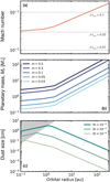 |
Fig. A.1 Mach number, planetary mass, and the dust size as a function of the orbital radius. The gray shaded region in panel c denotes the Stokes regime. |
Appendix A.2 Orbital radius of the planet
When we convert a dimensionless quantity into a dimensionless one, we need to determine the orbital distance of the planet, rp. To do this, we specify rp based on the value of the Mach number of the headwind, ℳhw.
From Eq. (A.4), the Mach number of the headwind is given by:
 (A.10)
where we set d ln p/d ln r = −2.55 for the viscous heating regime and dln p/d ln r = −2.78 for the irradiation heating regime, respectively (Ida et al. 2016). From Eq. (A.10), we can set rp ≃ 1 au when ℳhw = 0.03 (rp ≃ 50 au when ℳhw = 0.1) as a reference value of the planet location (Fig. A.1a).
Appendix A.3 Planet mass
In the disk model given in Sect. A.1, the planet mass is calculated by:
 (A.11)
 (A.12)
 (A.13)
The pebble isolation mass is given by (Bitsch et al. 2018):
![${M_{{\rm{iso}}}} = 25{M_ \oplus }{\left( {{h \over {0.05}}} \right)^3}\left[ {0.34{{\left( {{3 \over {\log {\alpha _{{\rm{diff }}}}}}} \right)}^4} + 0.66} \right].$](/articles/aa/full_html/2024/12/aa51159-24/aa51159-24-eq116.png) (A.14)
(A.14)
Figure A.1b shows Mp for different m as a function of the orbital radius.
Appendix A.4 Dust size
From Eq. (4), the physical size of dust, s, is calculated by:
 (A.15)
In Eq. (A.15), we used the following equations for the stopping time of dust:
 (A.16)–(A.17)
where ρ• = 2 g/cm3 is the internal density of dust and σmol = 2 × 10⁻¹⁵ cm2 is the molecular collision cross section.
In our disk model, the gas drag regime switches from the Stokes to the Epstein regime when St ≤ 6.6 × 10⁻³ at rp = 1 au (St ≤ 2.2 × 10³ at 50 au). In the Epstein regime, we have
 (A.18)–(A.19)
Figure A.1c shows the dust size for different St as a function of the orbital radius.
Appendix A.5 Time
The orbital period is given by:
 (A.20)
where t is the dimensionless time in our simulations.
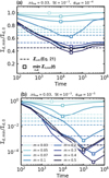 |
Fig. A.2 Time evolution of the minimum dust surface density for different planetary masses. We fixed the Stokes number and the Mach number St = 10−3 and ℳhw = 0.03. We set αdiff = 10−4 in panel a and αdiff = 10−5 in panel b. The square symbols denote the global minimum of Σd,min(t). The horizontal dashed lines mark Σcrit (Eq. 21). |
Appendix A.6 Length scale
For each dust surface density simulation, we used a 1D simulation domain with the constant spatial intervals, Δx = 0.01 H (Sect. 2.4). For a given orbital distance of the planet, rp, we convert the units of the grid cell from H to au based on the following methods. We defined the radial distance of the i-th grid from the central star in au units as ri, where i = 0 corresponds to the planet location and i = 1, 2, … (i = −1, −2, …) corresponds to the position outside (inside) the planetary orbit. Assuming that the disk aspect ratio is constant, we computed ri by the following equation:
 (A.21)
 (A.22)
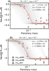 |
Fig. A.3 Global minimum of the dust surface density as a function of the planetary mass. We fixed the Stokes number St = 10−3. We set αdiff = 10−4 in panel a and αdiff = 10−5 in panel b. Different symbols correspond to different Mach numbers. The red solid line is the fitting formula for the numerical results of ℳhw = 0.03 (Eq. B.4). The gray thin lines show the uncertainties of Eq. (B.4). |
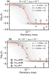 |
Fig. A.4 Steady-state dust gap depth as a function of the planetary mass. We fixed the Stokes number St = 10−3. We set αdiff = 10−4 in panel a and αdiff = 10−5 in panel b. Different symbols correspond to different Mach numbers. The red solid line is the fitting formula for the numerical results of ℳhw = 0.03 (Eq. B.9). The gray thin lines show the uncertainties of Eq. (B.9). |
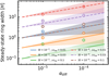 |
Fig. A.5 Steady-state dust ring width as a function of the turbulent parameter. The numerical results for different planetary masses were averaged and plotted with the circle symbols. The solid and dashed lines are given by Eq. (B.12). The shaded regions show the uncertainties. |
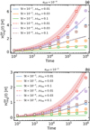 |
Fig. A.6 Time-dependent dust ring width as a function of time. The numerical results for different planetary masses were averaged and plotted with the square symbols. The solid and dashed lines are given by Eq. (B.13). The shaded regions show the uncertainties. |
Appendix B Fitting formulae for  ,
, , and
, and 
We introduce the fitting formulae for the global minimum of the time-dependent dust surface density,  the steady-state dust gap depth,
  , and the steady-state dust ring width,
  . For the fitting processes, we used the numerical results of St ≤ 10−3.
Figure A.2 shows the time evolution of the minimum dust surface density for different planetary masses, Σd,min(t), obtained from our numerical simulations. The minimum dust surface density has the complex dependence on time. We marked the global minimum of the time-dependent dust surface density,  , with the square symbol in Fig. A.2. We considered that when
  the dust gap expands with time (Sect. 4.1).
Figure A.3 shows  as a function of the planetary mass. We found that the dependence of min
  on the Mach number is weak. Thus, for the fitting process we used the numerical results of ℳhw = 0.03 as the representative value.
We assumed that the numerical result can be fitted by the following sigmoid curve:
 (B.1)
(B.1)
Using the scipy.optimize.curve_fit library of python, we constrained the fitting coefficients in Eq. (B.1): a, b, and c. We obtained
 (B.2)
(B.2)

when αdiff = 10−5. From Eqs. (B.2) and (B.3), we obtained
 (B.4)
(B.4)
where we used the best fit values of the fitting coefficients. Equation (B.1) gives  when αdiff ≳ 10−4, which is unphysical.
Thus, we set the upper limit and obtained the semi-analytic formula for the global minimum of the dust surface density:
 (B.5)
(B.5)
We plotted Eq. (B.5) in Fig. A.3 with the solid line.
Figure A.4 shows the steady-state dust gap depth as a function of the planetary mass. Similar to the fitting process of we used the numerical results of ℳhw = 0.03 as the representative value for the fitting and assumed that the numerical result can be fitted by:
 (B.6)
(B.6)
Using the scipy.optimize.curve_fit library, we obtained the fitting coefficients a′, b′, and c′ as follows:
 (B.7)
(B.7)

when αdiff = 10−5. From Eqs. (B.7) and (B.11), we obtained
 (B.9)
(B.9)
Equation (B.6) gives  when αdiff ≳ 10−4. To avoid unphysical solutions, we set the upper limit:
 (B.10)
We plotted Eq. (B.10) in Fig. A.4 with the solid line.
Figure A.5 shows the steady-state dust ring width as a function of αdiff. As shown in Fig. 15, the dust ring width is weakly dependent on the planetary mass. Thus, we averaged the numerical results for different planetary masses and plotted them in Fig. A.5 with the circle symbols. We assumed that the steady-state dust ring width is proportional to the characteristic length in which the drift timescale coincides with the diffusion timescale, ℒeq (Eq. 9):  . With the least-squares method, we derived the coefficient:
 (B.11)

We plotted Eq. (B.12) in Fig. A.5 with the solid lines.
Figure A.6 shows the dust ring width as a function of time. Since the dust ring width is weakly dependent on the planetary mass, same as in Fig. A.5, we averaged the numerical results for different planetary masses at each time and then plotted them in Fig. A.6 with the squares symbols. We assumed that the time-dependent dust ring width can be fitted by the following sigmoid curve:
 (B.13)
With the least-squares method, we determined the power of (t/τring)q: q = 0.42 ± 0.045. We plotted Eq. (B.13) in Fig. A.6 with the solid lines.
References
- ALMA Partnership (Brogan, C. L., et al.) 2015, ApJ, 808, L3 [Google Scholar]
- Andrews, S. M., Huang, J., Pérez, L. M., et al. 2018, ApJ, 869, L41 [NASA ADS] [CrossRef] [Google Scholar]
- Bae, J., Isella, A., Zhu, Z., et al. 2023, in Astronomical Society of the Pacific Conference Series, 534, 423 [NASA ADS] [Google Scholar]
- Bai, X.-N., & Stone, J. M. 2013, ApJ, 769, 76 [Google Scholar]
- Bailey, A., Stone, J. M., & Fung, J. 2021, ApJ, 915, 113 [NASA ADS] [CrossRef] [Google Scholar]
- Bitsch, B., Morbidelli, A., Johansen, A., et al. 2018, A&A, 612, A30 [NASA ADS] [CrossRef] [EDP Sciences] [Google Scholar]
- Blum, J., & Wurm, G. 2008, Annu. Rev. Astron. Astrophys., 46, 21 [CrossRef] [Google Scholar]
- Burrill, B. P., Ricci, L., Harter, S. K., Zhang, S., & Zhu, Z. 2022, ApJ, 928, 40 [NASA ADS] [CrossRef] [Google Scholar]
- Carpenter, J., Iono, D., Kemper, F., & Wootten, A. 2020, arXiv e-prints [arXiv:2001.11076] [Google Scholar]
- Dipierro, G., & Laibe, G. 2017, MNRAS, 469, 1932 [Google Scholar]
- Dipierro, G., Laibe, G., Price, D. J., & Lodato, G. 2016, MNRAS, 459, L1 [NASA ADS] [CrossRef] [Google Scholar]
- Doi, K., & Kataoka, A. 2023, ApJ, 957, 11 [CrossRef] [Google Scholar]
- Dong, R., & Fung, J. 2017, ApJ, 835, 146 [NASA ADS] [CrossRef] [Google Scholar]
- Dong, R., Li, S., Chiang, E., & Li, H. 2018, ApJ, 866, 110 [NASA ADS] [CrossRef] [Google Scholar]
- Drazkowska, J., Bitsch, B., Lambrechts, M., et al. 2023, in Astronomical Society of the Pacific Conference Series, 534, 717 [Google Scholar]
- Dullemond, C. P., Birnstiel, T., Huang, J., et al. 2018, ApJ, 869, L46 [NASA ADS] [CrossRef] [Google Scholar]
- Emsenhuber, A., Mordasini, C., Burn, R., et al. 2021, A&A, 656, A69 [NASA ADS] [CrossRef] [EDP Sciences] [Google Scholar]
- Fernandes, R. B., Mulders, G. D., Pascucci, I., Mordasini, C., & Emsenhuber, A. 2019, ApJ, 874, 81 [NASA ADS] [CrossRef] [Google Scholar]
- Francis, L., & van der Marel, N. 2020, ApJ, 892, 111 [Google Scholar]
- Fressin, F., Torres, G., Charbonneau, D., et al. 2013, ApJ, 766, 81 [NASA ADS] [CrossRef] [Google Scholar]
- Fulton, B. J., Rosenthal, L. J., Hirsch, L. A., et al. 2021, ApJS, 255, 14 [NASA ADS] [CrossRef] [Google Scholar]
- Fung, J., Artymowicz, P., & Wu, Y. 2015, ApJ, 811, 101 [Google Scholar]
- Gammie, C. F. 2001, ApJ, 553, 174 [Google Scholar]
- Garaud, P., & Lin, D. 2007, ApJ, 654, 606 [NASA ADS] [CrossRef] [Google Scholar]
- Gonzalez, J.-F., Laibe, G., & Maddison, S. T. 2017, MNRAS, 467, 1984 [NASA ADS] [Google Scholar]
- Goodman, J., & Rafikov, R. 2001, ApJ, 552, 793 [NASA ADS] [CrossRef] [Google Scholar]
- Guerra-Alvarado, O. M., Carrasco-González, C., Macías, E., et al. 2024, A&A, 686, A298 [NASA ADS] [CrossRef] [EDP Sciences] [Google Scholar]
- Güttler, C., Blum, J., Zsom, A., Ormel, C. W., & Dullemond, C. P. 2010, A&A, 513, A56 [Google Scholar]
- Haisch, Karl E., J., Lada, E. A., & Lada, C. J. 2001, ApJ, 553, L153 [Google Scholar]
- Harter, S. K., Ricci, L., Zhang, S., & Zhu, Z. 2020, ApJ, 905, 24 [NASA ADS] [CrossRef] [Google Scholar]
- Huang, J., Andrews, S. M., Dullemond, C. P., et al. 2018, ApJ, 869, L42 [NASA ADS] [CrossRef] [Google Scholar]
- Ida, S., Guillot, T., & Morbidelli, A. 2016, A&A, 591, A72 [NASA ADS] [CrossRef] [EDP Sciences] [Google Scholar]
- Jiang, H., Zhu, W., & Ormel, C. W. 2022, ApJ, 924, L31 [NASA ADS] [CrossRef] [Google Scholar]
- Jiang, H., Macías, E., Guerra-Alvarado, O. M., & Carrasco-González, C. 2024, A&A, 682, A32 [NASA ADS] [CrossRef] [EDP Sciences] [Google Scholar]
- Jiménez, M. A., & Masset, F. S. 2017, MNRAS, 471, 4917 [Google Scholar]
- Kanagawa, K. D., Muto, T., & Tanaka, H. 2021, ApJ, 921, 169 [NASA ADS] [CrossRef] [Google Scholar]
- Kurokawa, H., & Tanigawa, T. 2018, MNRAS, 479, 635 [Google Scholar]
- Kuwahara, A., & Kurokawa, H. 2020, A&A, 633, A81 [NASA ADS] [CrossRef] [EDP Sciences] [Google Scholar]
- Kuwahara, A., & Kurokawa, H. 2024, A&A, 682, A14 [NASA ADS] [CrossRef] [EDP Sciences] [Google Scholar]
- Kuwahara, A., Kurokawa, H., & Ida, S. 2019, A&A, 623, A179 [NASA ADS] [CrossRef] [EDP Sciences] [Google Scholar]
- Kuwahara, A., Kurokawa, H., Tanigawa, T., & Ida, S. 2022, A&A, 665, A122 [NASA ADS] [CrossRef] [EDP Sciences] [Google Scholar]
- Lambrechts, M., Johansen, A., & Morbidelli, A. 2014, A&A, 572, A35 [NASA ADS] [CrossRef] [EDP Sciences] [Google Scholar]
- Liu, B., Johansen, A., Lambrechts, M., Bizzarro, M., & Haugbølle, T. 2022, Sci. Adv., 8, eabm3045 [NASA ADS] [CrossRef] [Google Scholar]
- Lodato, G., Dipierro, G., Ragusa, E., et al. 2019, MNRAS, 486, 453 [Google Scholar]
- Long, F., Pinilla, P., Herczeg, G. J., et al. 2018, ApJ, 869, 17 [Google Scholar]
- Luhman, K., Allen, P., Espaillat, C., Hartmann, L., & Calvet, N. 2009, ApJS, 186, 111 [Google Scholar]
- Lynden-Bell, D., & Pringle, J. E. 1974, MNRAS, 168, 603 [Google Scholar]
- Mordasini, C., Deeg, H., & Belmonte, J. 2018, Handbook of Exoplanets (Cham: Springer), 143 [Google Scholar]
- Mulders, G. D., Pascucci, I., Ciesla, F. J., & Fernandes, R. B. 2021, ApJ, 920, 66 [NASA ADS] [CrossRef] [Google Scholar]
- Müller-Horn, J., Pichierri, G., & Bitsch, B. 2022, A&A, 663, A163 [NASA ADS] [CrossRef] [EDP Sciences] [Google Scholar]
- Musiolik, G., Teiser, J., Jankowski, T., & Wurm, G. 2016a, ApJ, 818, 16 [Google Scholar]
- Musiolik, G., Teiser, J., Jankowski, T., & Wurm, G. 2016b, ApJ, 827, 63 [NASA ADS] [CrossRef] [Google Scholar]
- Muto, T., & Inutsuka, S.-i. 2009, ApJ, 695, 1132 [NASA ADS] [CrossRef] [Google Scholar]
- Nakagawa, Y., Sekiya, M., & Hayashi, C. 1986, Icarus, 67, 375 [Google Scholar]
- Ndugu, N., Bitsch, B., & Jurua, E. 2019, MNRAS, 488, 3625 [CrossRef] [Google Scholar]
- Oka, A., Nakamoto, T., & Ida, S. 2011, ApJ, 738, 141 [Google Scholar]
- Okuzumi, S., & Tazaki, R. 2019, ApJ, 878, 132 [Google Scholar]
- Ormel, C. W., Shi, J.-M., & Kuiper, R. 2015, MNRAS, 447, 3512 [Google Scholar]
- Paardekooper, S.-J., & Mellema, G. 2006, A&A, 453, 1129 [CrossRef] [EDP Sciences] [Google Scholar]
- Pierens, A., Lin, M.-K., & Raymond, S. N. 2019, MNRAS, 488, 645 [NASA ADS] [CrossRef] [Google Scholar]
- Ribas, Á., Clarke, C. J., & Zagaria, F. 2024, MNRAS, 532, 1752 [NASA ADS] [CrossRef] [Google Scholar]
- Rice, W., Armitage, P. J., Wood, K., & Lodato, G. 2006, MNRAS, 373, 1619 [CrossRef] [Google Scholar]
- Ricci, L., Liu, S.-F., Isella, A., & Li, H. 2018, ApJ, 853, 110 [NASA ADS] [CrossRef] [Google Scholar]
- Rosotti, G. P., Juhasz, A., Booth, R. A., & Clarke, C. J. 2016, MNRAS, 459, 2790 [Google Scholar]
- Selina, R. J., Murphy, E. J., McKinnon, M., et al. 2018, Sci. Next Gener. Very Large Array, 517, 15 [Google Scholar]
- Shakura, N. I., & Sunyaev, R. A. 1973, A&A, 24, 337 [NASA ADS] [Google Scholar]
- Sierra, A., Pérez, L. M., Zhang, K., et al. 2021, ApJS, 257, 14 [NASA ADS] [CrossRef] [Google Scholar]
- Stone, J. M., Tomida, K., White, C. J., & Felker, K. G. 2020, ApJS, 249, 4 [NASA ADS] [CrossRef] [Google Scholar]
- Tanaka, H., & Ward, W. R. 2004, ApJ, 602, 388 [Google Scholar]
- Tanaka, H., Takeuchi, T., & Ward, W. R. 2002, ApJ, 565, 1257 [Google Scholar]
- Tzouvanou, A., Bitsch, B., & Pichierri, G. 2023, A&A, 677, A82 [NASA ADS] [CrossRef] [EDP Sciences] [Google Scholar]
- Ueda, T., Tazaki, R., Okuzumi, S., Flock, M., & Sudarshan, P. 2024, Nat. Astron., 8, 1148 [NASA ADS] [CrossRef] [Google Scholar]
- van der Marel, N., & Mulders, G. D. 2021, AJ, 162, 28 [NASA ADS] [CrossRef] [Google Scholar]
- Vericel, A., & Gonzalez, J.-F. 2020, MNRAS, 492, 210 [NASA ADS] [CrossRef] [Google Scholar]
- Vericel, A., Gonzalez, J.-F., Price, D. J., Laibe, G., & Pinte, C. 2021, MNRAS, 507, 2318 [NASA ADS] [CrossRef] [Google Scholar]
- Villenave, M., Stapelfeldt, K., Duchêne, G., et al. 2022, ApJ, 930, 11 [NASA ADS] [CrossRef] [Google Scholar]
- Wang, S., Kanagawa, K. D., & Suto, Y. 2021, ApJ, 923, 165 [NASA ADS] [CrossRef] [Google Scholar]
- Ward, W. R. 1986, Icarus, 67, 164 [Google Scholar]
- Weber, P., Benítez-Llambay, P., Gressel, O., Krapp, L., & Pessah, M. E. 2018, ApJ, 854, 153 [NASA ADS] [CrossRef] [Google Scholar]
- Weidenschilling, S. J. 1977, Ap&SS, 51, 153 [Google Scholar]
- Weiss, L. M., & Marcy, G. W. 2014, ApJ, 783, L6 [Google Scholar]
- Yang, C.-C., & Zhu, Z. 2020, MNRAS, 491, 4702 [NASA ADS] [CrossRef] [Google Scholar]
- Youdin, A. N., & Lithwick, Y. 2007, Icarus, 192, 588 [NASA ADS] [CrossRef] [Google Scholar]
- Zhang, S., Zhu, Z., Huang, J., et al. 2018, ApJ, 869, L47 [Google Scholar]
- Zhang, K., Booth, A. S., Law, C. J., et al. 2021, ApJS, 257, 5 [NASA ADS] [CrossRef] [Google Scholar]
- Zhang, S., Kalscheur, M., Long, F., et al. 2023, ApJ, 952, 108 [NASA ADS] [CrossRef] [Google Scholar]
- Zhu, Z., Nelson, R. P., Dong, R., Espaillat, C., & Hartmann, L. 2012, ApJ, 755, 6 [Google Scholar]
- Zhu, Z., Stone, J. M., Rafikov, R. R., & Bai, X.-n. 2014, ApJ, 785, 122 [NASA ADS] [CrossRef] [Google Scholar]
- Zsom, A., Ormel, C. W., Güttler, C., Blum, J., & Dullemond, C. 2010, A&A, 513, A57 [NASA ADS] [CrossRef] [EDP Sciences] [Google Scholar]
We used a slightly different definition of the dust gap width with respect to Dong & Fung (2017), in which the authors calculated the geometric mean of the minimum and initial dust surface densities,  .
.
Equation (28) is an analytic solution to the following logistic equation
 (27)
(27)
All Tables
All Figures
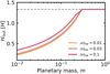 |
Fig. 1 Width of the outflow region as a function of the planetary mass (Eq. (12)). |
| In the text | |
|
Fig. 2 Definition of the widths of the dust ring and gap. The red and yellow shaded regions show the numerically calculated widths of the dust ring and gap. The circles mark Σd,max and Σd,min. |
| In the text | |
|
Fig. 3 Perturbation of the planet-induced gas flow on the radial velocity of dust and the dust surface density. We set m = 0.1, ℳhw = 0.03, St = 10−3, and αdiff = 10−4. Top: gas flow structure at the meridian plane. The color contour represents the gas velocity in the x-direction averaged in the y-direction within the calculation domain of hydrodynamical simulation, 〈vx,g〉y. The vertical dotted lines represent the x-coordinates of the edges of the outflow region, |
| In the text | |
|
Fig. 4 Time evolution of the dust surface density in low-turbulence disks. We set m = 0.1, ℳhw = 0.03, St = 10−3, and αdiff = 10−5. The horizontal axis is on a log scale, whose range is extended to x ∈ [−100, 5]. The vertical dashed lines show the analytic model of the location of the inner edge of the dust gap, which moves with vdrift (Sect. 4.4). |
| In the text | |
|
Fig. 5 Time evolution of Σd(t) in the two-dimensional plane. We set m = 0.1, ℳhw = 0.03, St = 10−3, and αdiff = 10−5. These images were generated based on the results of 1D calculations assuming an axisymmetric dust distribution, neglecting disk curvature. The axes are normalized by the planet location, rp, calculated by X = Y = (r − rp)/hp, where r is the radial coordinate centered at the star and hp is the disk aspect ratio at r = rp. We set hp = 0.05. |
| In the text | |
|
Fig. 6 Cavity-filling timescale. We only focus on m ≥ 0.1 in which the dust cavities form. |
| In the text | |
|
Fig. 7 Dependence of Σd(t) on the planetary mass. We set ℳhw = 0.03, St = 10−3, and αdiff = 10−5. The vertical dotted lines correspond to |x| = 4/3 (the x-coordinate of the edge of the outflow region for m ≳ 0.3; Eq. (12)). The small panels above the upper left corners of panels a-c are the zoomed-in views for m = 0.03, 0.05, and 0.07. |
| In the text | |
|
Fig. 8 Dependence of Σd(t) on the Mach number of the headwind. We set m = 0.2, St = 10−3, and αdiff = 10−4. We varied the Mach number of the headwind in each panel, ℳhw = 0.01 (top) and ℳhw = 0.1 (bottom). |
| In the text | |
|
Fig. 9 Dependence of Σd(t) on the Stokes number. We set m = 0.1, ℳhw = 0.03, and αdiff = 10–5. The vertical dotted lines correspond to |
| In the text | |
|
Fig. 10 Summary of the parameter dependence of Σd(t). We set ℳhw = 0.03 and t = 105. We varied the planetary mass, the Stokes number, and the turbulent parameter. |
| In the text | |
|
Fig. 11 Contour plot of the dust gap depth as a function of the planetary mass and the Stokes number. We set ℳhw = 0.03 and t = 105. We varied the turbulent parameter in each panel, αdiff = 10–4 (panel a) and αdiff = 10–5 (panel b). |
| In the text | |
|
Fig. 12 Time evolution of the dust gap width for different planetary masses. We fixed the Stokes number St = 10–3 and the Mach number ℳhw = 0.03, and set αdiff = 10–4 in panel a and αdiff = 10–5 in panel b. The solid lines with the circle symbols and the dashed lines are the numerically calculated and the semi-analytic dust gap widths, respectively (Eq. (26); Sect. 4.4). We note that in panels a and b, the numerically calculated dust gap width for m = 0.03 is not shown because we obtained |
| In the text | |
|
Fig. 13 Time evolution of the dust gap depth for different planetary masses. We fixed the Stokes number St = 10–3 and the Mach number ℳhw = 0.03, and set αdiff = 10–4 in panel a and αdiff = 10–5 in panel b. The solid lines with the circle symbols and the dashed lines are the numerically calculated and the semi-analytic dust gap depths, respectively (Eq. (28); Sect. 4.4). |
| In the text | |
|
Fig. 14 Dust gap depth as a function of planetary mass at t = 106. We fixed the Stokes number St = 10–3 and set αdiff = 10–4 in panel a and αdiff = 10–5 in panel b. The solid lines with the circle symbols and the dashed lines are the numerically calculated and the semi-analytic dust gap depths, respectively (Eq. (28); Sect. 4.4). |
| In the text | |
|
Fig. 15 Time evolution of the dust ring width for different planetary masses. The assumed parameters (ℳhw, St, and αdiff) are shown at the top of each panel. The solid lines with the circle symbols and the dashed lines are the numerically calculated and the semi-analytic dust ring widths, respectively (Eq. (33); Sect. 4.4). |
| In the text | |
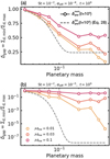 |
Fig. 16 Same as Fig. 14, but for St = 10–2. |
| In the text | |
|
Fig. 17 Time-dependent dust surface density with particle sizes of s = 3.7 mm perturbed by an Earth-like planet (Mp = 0.66M⊕) at 1 au. Numerical simulations were conducted in dimensionless units. We set m = 0.1, ℳhw = 0.03, St = 10–3, and varied the turbulent parameter in each panel, αdiff = 10–5 (panel a) and αdiff = 10–4 (panel b). For the assumed parameter set, the pebble isolation masses are given by Miso = 2.8 M⊗ (panel a) and 3 M⊗ (panel b; Eq. (A.14)). |
| In the text | |
|
Fig. 18 Time-dependent dust surface density with particle sizes of s = 0.23 mm for a Neptune-like planet (Mp = 13 M⊗) at 50 au. The numerical simulations were conducted in dimensionless units. We set m = 0.1, ℳhw = 0.1, St = 3 × 10⁻³, and varied the turbulent parameter in each panel, αdiff = 10–5 (panel a) and αdiff = 10–4 (panel b). For the assumed parameter set, the pebble isolation masses are given by Miso = 56 M⊗ (panel a) and 60 Mæ (panel b; Eq. (A.14)). |
| In the text | |
|
Fig. 19 Dust gap width as a function of the dust gap location. We set St = 10−3 and ℳhw = 0.03, and varied the turbulent parameter in each panel, αdiff = 10−4 (panel a) and αdiff = 10−5 (panel b). The blue and orange solid lines denote H and 5 H, respectively (Eq. (A.3)). Panel a: Blue shaded region given by |
| In the text | |
|
Fig. 20 Dust ring width as a function of the ring location. We set ℳhw = 0.03 and αdiff = 10−4. The dashed and dotted lines are given by Eq. (33) with St = 10−3 and 10−4, where we converted the units of |
| In the text | |
|
Fig. A.1 Mach number, planetary mass, and the dust size as a function of the orbital radius. The gray shaded region in panel c denotes the Stokes regime. |
| In the text | |
|
Fig. A.2 Time evolution of the minimum dust surface density for different planetary masses. We fixed the Stokes number and the Mach number St = 10−3 and ℳhw = 0.03. We set αdiff = 10−4 in panel a and αdiff = 10−5 in panel b. The square symbols denote the global minimum of Σd,min(t). The horizontal dashed lines mark Σcrit (Eq. 21). |
| In the text | |
|
Fig. A.3 Global minimum of the dust surface density as a function of the planetary mass. We fixed the Stokes number St = 10−3. We set αdiff = 10−4 in panel a and αdiff = 10−5 in panel b. Different symbols correspond to different Mach numbers. The red solid line is the fitting formula for the numerical results of ℳhw = 0.03 (Eq. B.4). The gray thin lines show the uncertainties of Eq. (B.4). |
| In the text | |
|
Fig. A.4 Steady-state dust gap depth as a function of the planetary mass. We fixed the Stokes number St = 10−3. We set αdiff = 10−4 in panel a and αdiff = 10−5 in panel b. Different symbols correspond to different Mach numbers. The red solid line is the fitting formula for the numerical results of ℳhw = 0.03 (Eq. B.9). The gray thin lines show the uncertainties of Eq. (B.9). |
| In the text | |
|
Fig. A.5 Steady-state dust ring width as a function of the turbulent parameter. The numerical results for different planetary masses were averaged and plotted with the circle symbols. The solid and dashed lines are given by Eq. (B.12). The shaded regions show the uncertainties. |
| In the text | |
|
Fig. A.6 Time-dependent dust ring width as a function of time. The numerical results for different planetary masses were averaged and plotted with the square symbols. The solid and dashed lines are given by Eq. (B.13). The shaded regions show the uncertainties. |
| In the text | |
Current usage metrics show cumulative count of Article Views (full-text article views including HTML views, PDF and ePub downloads, according to the available data) and Abstracts Views on Vision4Press platform.
Data correspond to usage on the plateform after 2015. The current usage metrics is available 48-96 hours after online publication and is updated daily on week days.
Initial download of the metrics may take a while.