| Issue |
A&A
Volume 683, March 2024
|
|
|---|---|---|
| Article Number | A82 | |
| Number of page(s) | 9 | |
| Section | Cosmology (including clusters of galaxies) | |
| DOI | https://doi.org/10.1051/0004-6361/202348643 | |
| Published online | 08 March 2024 | |
The splashback radius and the radial velocity profile of galaxy clusters in IllustrisTNG
1
Department of Astronomy and Physics, Saint Mary’s University, 923 Robie Street, Halifax B3H3C3, Canada
e-mail: This email address is being protected from spambots. You need JavaScript enabled to view it.
2
Smithsonian Astrophysical Observatory, 60 Garden Street, Cambridge 02138, USA
Received:
17
November
2023
Accepted:
16
January
2024
Abstract
We used 1697 clusters of galaxies from the TNG300-1 simulation (mass M200c > 1014 M⊙ and redshift range 0.01 ≤ z ≤ 1.04) to explore the physics of the cluster infall region. We used the average radial velocity profile derived from simulated galaxies, vrad(r), and the average velocity dispersion of galaxies at each redshift, σv(r), to explore cluster-centric dynamical radii that characterize the cluster infall region. We revisited the turnaround radius, the limiting outer radius of the infall region, and the radius where the infall velocity has a well-defined minimum. We also explored two new characteristic radii: (i) the point of inflection of vrad(r) that lies within the velocity minimum, and (ii) the smallest radius where σv(r) = |vrad(r)|. These two, nearly coincident, radii mark the inner boundary of the infall region where radial infall ceases to dominate the cluster dynamics. Both of these galaxy velocity based radii lie within 1σ of the observable splashback radius. The minimum in the logarithmic slope of the galaxy number density is an observable proxy for the apocentric radius of the most recently accreted galaxies, the physical splashback radius. The two new dynamically derived radii relate the splashback radius to the inner boundary of the cluster infall region.
Key words: methods: numerical / galaxies: clusters: general / galaxies: kinematics and dynamics
© The Authors 2024
 Open Access article, published by EDP Sciences, under the terms of the Creative Commons Attribution License (https://creativecommons.org/licenses/by/4.0), which permits unrestricted use, distribution, and reproduction in any medium, provided the original work is properly cited.
This article is published in open access under the Subscribe to Open model. This email address is being protected from spambots. You need JavaScript enabled to view it. to support open access publication.
1. Introduction
Clusters of galaxies are massive self-gravitating systems of galaxies comprised of a dense central region in approximate virial equilibrium surrounded by an extended region where continuing infall dominates the dynamics. The infall region extends to scales ≲10 Mpc (Geller et al. 1999; Rines & Diaferio 2006; Rines et al. 2013; Umetsu et al. 2014, 2016, 2020). Across this large volume, clusters present distinctive dynamical regimes. Characteristic dynamical radii mark the transition between the virial and infall regions. These radii inform comparisons with models of formation and evolution of cluster of galaxies (e.g., Press & Schechter 1974; White & Rees 1978; Bower 1991; Lacey & Cole 1993; Sheth & Tormen 2002; Zhang et al. 2008; Corasaniti & Achitouv 2011; De Simone et al. 2011; Achitouv et al. 2014; Musso et al. 2018).
In standard cosmology, the turnaround radius is the outer boundary of a cluster; it marks the radius where matter decouples from the Hubble flow. Within the turnaround, the gravitational potential of the cluster dominates the dynamics (Gunn et al. 1972; Silk 1974; Schechter 1980; Bertschinger 1985; Villumsen & Davis 1986; Cupani et al. 2008, 2011). Because the matter overdensity is small averaged over the volume within the turnaround radius, quasi-linear dynamics predicts the turnaround radius accurately.
Within the turnaround radius, clusters have an extended accretion region often referred to as the infall region. Here, there is a net radial infall of matter onto the cluster. The radial velocity in this region is negative, and the well-defined minimum of the radial velocity profile is a proxy for the radius where the infall is strongest (Cuesta et al. 2008; De Boni et al. 2016; Vallés-Pérez et al. 2020; Pizzardo et al. 2021, 2023b; Fong & Han 2021; Gao et al. 2023). Fong & Han (2021) and Gao et al. (2023) recently proposed two additional characteristic radii in the infall region. They define an inner depletion radius where the mass flow rate is maximum. This radius is similar to the radius where the radial velocity has a minimum. They also define a characteristic depletion radius at slightly larger cluster-centric distance which traces the region where clustering around the halo is weakest relative to clustering around a random matter particle.
In the dense central regions of galaxy clusters, orbital motions dominate infall. The limiting radius of this approximately virialized region, the virial radius (e.g. Gunn et al. 1972; Peebles 1980; Lacey & Cole 1993), typically defines the cluster size. Proxies for the virial radius include R200c and R200 m, where RΔ is the cluster-centric distance that encloses a mean density Δc times the critical density or Δm times the mean background density (Lacey & Cole 1993).
A more recently suggested boundary of the inner region of a cluster is the splashback radius, Rspl, defined as the first apocenter of orbits of recently accreted material (Adhikari et al. 2014; Diemer & Kravtsov 2014; More et al. 2015; Diemer 2020). The splashback radius marks a natural boundary where the internal cluster dynamics dominates over systematic infall. Detailed studies use N-body simulations to explore the trajectories of individual dark matter particles as a theoretical proxy of Rspl (e.g. Diemer & Kravtsov 2014; Diemer et al. 2017; Mansfield et al. 2017; Diemer 2018; Xhakaj et al. 2020). Usually, Rspl is outside the virialized radius of a cluster, ∼1.5 − 2R200c. At fixed redshift, Rspl decreases with increasing halo mass accretion rate. At fixed mass accretion rate, Rspl increases with increasing redshift.
Adhikari et al. (2014) show that at ∼Rspl particles generate caustics in phase-space density. They match this caustic to a sudden drop in the logarithmic derivative of the mass density profile of halos (Diemer & Kravtsov 2014). This feature in the mass (or number) density profile of halos,  (
( ), is an observable proxy for Rspl. In fact, a variety of observations detect the minimum in the logarithmic slope of cluster density associated with Rspl (More et al. 2016; Baxter et al. 2017; Chang et al. 2018; Shin et al. 2019; Zürcher & More 2019; Murata et al. 2020; Adhikari et al. 2021; Bianconi et al. 2021; Gonzalez et al. 2021).
So far, the physical meaning of Rspl relies solely on the dynamics of dark matter particles from pure N-body simulations. Studies based on hydrodynamical simulations investigate Rspl through its proxies,  or
or  (Baxter et al. 2021; Deason et al. 2021; O’Neil et al. 2021; O’Neil et al. 2022; Dacunha et al. 2022). Here we use the IllustrisTNG hydrodynamical simulations (Pillepich et al. 2018; Springel et al. 2018; Nelson et al. 2019) to interpret Rspl based on the dynamics of simulated galaxies rather than dark matter particles. Connecting Rspl directly to galaxy dynamics provides a way to unveil how galaxies as well as matter particles show clear signatures of the splashback physics.
The mean radial velocity profile of clusters in IllustrisTNG provides additional dimensions to the view of Rspl. The Rspl based on the matter density profile lies just within the radius where the radial velocity profile has a clear minimum. The radial velocity profile enables determination of two further characteristic radii: (1) the point of inflection inside the velocity minimum, and (2) the smallest radius where the local velocity dispersion exceeds the infall. From the turnaround radius inward, these two radii describe the radius where infall no longer dominates the dynamics. These two radii are essentially equal to the observable proxy of Rspl. This agreement extends the meaning of Rspl as the dynamical outer boundary of the region where orbital motions, as opposed to infall, dominate galaxy cluster dynamics.
Currently, these two galaxy radial velocity based radii are not directly observable. However, Odekon et al. (2022) show that data including independent distance measurements for galaxies around clusters and filaments allow extraction of the galaxy velocity field in the infall region.
Section 2.1 describes the IllustrisTNG simulations and the resulting cluster samples. Section 2.2 discusses the mass and velocity profiles. Section 3 outlines the definition of cluster dynamical radii based on the radial velocity profile. Sections 3.1 and 3.2 summarize the main properties of the turnaround radius and the radial velocity minimum, respectively. In Sect. 3.3 we identify radii based on the radial velocity profile that closely approximate the observable proxy of Rspl from the galaxy number density profile. We discuss the impact of the mass distribution on the dynamical radii in Sect. 4.1, compare the galaxy and total matter velocities in Sect. 4.2, and conclude in Sect. 5. Table 1 defines the symbols used throughout the paper.
Symbol definitions.
2. Cluster samples, velocity, and mass profiles
We built a sample of galaxy clusters from the TNG300-1 run of the IllustrisTNG simulations Pillepich et al. (2018), Springel et al. (2018), Nelson et al. (2019). We derived mass and radial velocity profiles for these clusters. We briefly discuss the cluster sample in Sect. 2.1 and the profiles in Sect. 2.2.
2.1. Simulations and catalogs
The IllustrisTNG simulations (Pillepich et al. 2018; Springel et al. 2018; Nelson et al. 2019) are a set of gravo-magnetohydrodynamical simulations based on the ΛCDM model. Table 2 lists the cosmological parameters of the simulations. TNG300-1 is the baryonic run with the highest resolution among the runs with the largest simulated volumes. The simulation has a comoving box size of 302.6 Mpc. TNG300-1 contains 25003 dark matter particles with mass mDM = 5.88 × 10⁷ M⊙ and the same number of gas cells with average mass mb = 1.10 × 10⁷ M⊙.
Cosmological parameters for IllustrisTNG.
As in Pizzardo et al. (2023a) we used group catalogues compiled by the IllustrisTNG Collaboration to extract all of the Friends-of-Friends (FoF) groups in TNG300-1 with M200c > 1014 M⊙. There are 1697 clusters in the 11 redshift bins in the range 0.01 ≤ z ≤ 1.04. Table 3 summarizes the main properties of the 11 subsamples, including redshift, number of clusters, median, interquartile range, and the minimum and maximum of the mass M200c in each bin.
Cluster samples from TNG300-1.
The mass and redshift sampling we adopted is consistent with the selection in recent studies that use hydrodynamical simulations to explore the outer region of galaxy clusters (e.g Baxter et al. 2021; Deason et al. 2021; O’Neil et al. 2021; O’Neil et al. 2022; Dacunha et al. 2022). This sampling mimics characteristics of observational approaches that focus on cluster masses for systems typically at z ≲ 1 (Tamura et al. 2016; Ivezić et al. 2019; Marshall et al. 2019; Cornwell et al. 2022, 2023).
For each FoF halo, IllustrisTNG provides a list of subhalos from the Subfind algorithm (Springel et al. 2001). For clusters in Table 3, we extracted subhalos with stellar mass M⋆ > 108 M⊙ and within 10R200c of the center of the cluster halo. We identified these subhalos as cluster member galaxies.
Blue, orange, green, and red points in Fig. 1 show the relation between M200c and the comoving R200c for clusters in four redshift bins: z = 0.01, 0.31, 0.62, and z = 1.04, respectively. Colored squares with error bars show the median and the interquartile range for each sample.
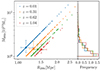 |
Fig. 1. Relation between M200c and comoving R200c for IllustrisTNG clusters. Left panel: Blue, orange, green, and red points show the M200c − R200c relation for clusters in four redshift bins z = 0.01, 0.31, 0.62, and z = 1.04, respectively. Colored squares with error bars show the median and interquartile range in each redshift bin. Right panel: Mass distribution histograms, with areas normalized to unity. |
Figure 1 and Table 3 show that, as the redshift increases from z = 0.01 to z = 1.04, the sample minimum M200c is nearly constant. The maximum M200c decreases by 71% with increasing redshift. The lower and upper extrema of the interquartile ranges of M200c behave in a similar way.
The mass functions in each bin are skewed towards low masses, M200c ≲ 3 × 10¹⁴ M⊙, even at low redshift. Thus even at low redshift the high-mass tails have small statistical weight. As the redshift increases from z = 0.01 to z = 1.04, the median M200c of clusters decreases by only 10%. The comoving R200c’s are proportional to  (Fig. 1).
2.2. Mass and velocity profiles
Pizzardo et al. (2023a) computed a cumulative mass profile for each cluster, M(< r), based on the 3D distribution of matter extracted from raw snapshots. These profiles include all matter species: dark matter, gas, stars, and black holes. For each cluster, Pizzardo et al. (2023a) computed M(< r) in 200 logarithmically spaced bins covering the radial range  . These profiles define R200c and M200c for each cluster; they allow straightforward computation of cumulative and shell density profiles for each cluster.
Pizzardo et al. (2023b) computed a single average galaxy radial velocity profile at each redshift by averaging over all the individual galaxy radial velocity profiles for the clusters in the redshift bin. They used a subsample of the cluster sample we used here, because they included only the 78% of systems allowing application of the caustic technique (Diaferio & Geller 1997; Diaferio 1999; Serra et al. 2011), an observational method for estimating the cluster mass profile. We included the entire set of IllustrisTNG clusters to maximize the sample size and to minimize any potential biases in the mass function and resulting radial velocity profile.
We computed the galaxy radial velocity profile of individual clusters in each subsample. Based on the comoving position of simulated galaxies with respect to the cluster center, rc, i, and the galaxy peculiar velocity, vp, i, we computed the radial velocity of each galaxy: vrad, i = [vp, i + H(zs)a(zs)rc, i] ⋅ rc, i/rc, i, where H(zs) and a(zs) are the Hubble function and the scale factor at the redshift zs of the snapshot. We computed the mean radial velocity profile of the cluster by averaging over the galaxy vrad(r)’s within 100 linearly spaced radial bins covering the range  . At each redshift, we averaged over all of the individual radial velocity profiles for the snapshot. We obtained a single mean galaxy radial velocity profile along with the dispersion around it.
The solid curves in Fig. 2 show the average galaxy radial velocity profiles for clusters at three redshifts z = 0.01, 0.62, and 1.04, from left to right, respectively. The dashed curves show Savitzky–Golay (Savitzky & Golay 1964) smoothed profiles derived with an 11 bin window and a fourth order polynomial interpolation. Shaded bands show the error in the smoothed profiles. Fluctuations and errors increase with increasing redshift because of the decreasing size of the cluster samples (see second column of Table 3).
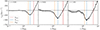 |
Fig. 2. Average radial velocity profiles and dynamical radii. Solid curves show the average galaxy radial velocity profiles of clusters at three redshifts: z = 0.01, 0.62, and 1.04, from left to right, respectively. Dashed curves show the Savitzky–Golay (Savitzky & Golay 1964) smoothed profiles. Shaded bands show the error in the smoothed profiles. In each panel, the red, blue, and orange lines show the turnaround, the minimum radial velocity, and the inflection point radii, respectively, derived from the average radial velocity profiles (see Sect. 3). |
3. Dynamical radii from radial velocity profiles
The galaxy radial velocity profile provides direct measures of both the turnaround radius and the infall velocity minimum for a cluster of galaxies. The radial velocity profile also provides a complementary view of the splashback radius Rspl as the inner boundary of the region where infalling galaxies dominate the cluster dynamics. We derive the turnaround radius and the point of minimum radial velocity in Sects. 3.1 and 3.2, respectively. Section 3.3, shows how these dynamically determined radii provide an interpretation of Rspl based on the radial velocity profile. We compare the dynamically derived radii with  , an observational proxy for Rspl (e.g. Adhikari et al. 2014; Diemer & Kravtsov 2014; More et al. 2015; Diemer 2017, 2018; Diemer et al. 2017; O’Neil et al. 2021).
3.1. The turnaround radius
The turnaround radius Rturn of a galaxy cluster is defined as the cluster-centric distance where galaxies depart from the Hubble flow (Gunn et al. 1972; Silk 1974; Schechter 1980). Hence Rturn is the radius where the smoothed galaxy radial velocity vrad(Rturn) = 0. The red vertical lines in Fig. 2 show the turnaround radius at redshifts z = 0.01, 0.62, and 1.04, respectively from left to right.
The red line in Fig. 3 shows Rturn in units of R200c as a function of redshift. The red shadowed band shows the uncertainty in Rturn, based on bootstrapping 1000 samples at each redshift. The radius Rturn is in the range (4.67 − 4.94)R200c, and it is independent of redshift with a typical value Rturn = (4.81 ± 0.10)R200c.
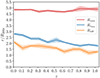 |
Fig. 3. Dynamical radii from smoothed average galaxy radial velocity profiles. The red, blue, and orange lines show the mass averaged turnaround radius (Sect. 3.1), the point of minimum vrad(r) (Sect. 3.2), and the inflection point of vrad(r) (Sect. 3.3), as a function of redshift, respectively. Shadowed bands show the error from bootstrap resampling of the correspondingly colored radius. |
We compared the Rturn values derived from the average radial velocity profile with the analytic predictions of Meiksin (1985; priv. comm. to Villumsen & Davis 1986),  . In this approach, the density contrast is δ(r) = 3M(r)/4πρbkgr3 − 1, where M(r) is the mass of the cluster within a distance r from the cluster center and ρbkg = Ωmρc is the background matter density. In the spherical collapse model, the radial velocity induced by the perturbation is
 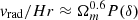 (Gunn et al. 1972; Silk 1974; Schechter 1980; Regos & Geller 1989). Meiksin’s approach approximates the function P(δ) with a non-polynomial; the overdensity within the turnaround radius where vrad/Hr = 1, is
 (1)
(1)
At each redshift, we computed the set of  ’s from the mass profiles of individual clusters in Table 3. We adopted the Lahav et al. (1991) approximation for the growth factor. At each redshift, we computed the median value
  and the interquartile range.
The radius Rturn derived from the average radial velocity profile is consistent with the analytic predictions of the Meiksin approximation. On average Rturn exceeds  by ≲3.9%. At each redshift, Rturn is within the interquartile range of the set of individual
  ’s, and Rturn and
  agree to within ∼1.5σ. The radius
  increases by ∼4% as the redshift increases from z = 0.01 to z = 1.04; this increase is not ruled out by the IllustrisTNG results.
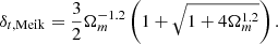
3.2. The minimum radial velocity
The point of minimum galaxy radial velocity, Rvmin, is a characteristic feature of the vrad(r) profiles. Previous evaluations of Rvmin include computations based on dark matter particles within stacked halo samples in N-body simulations (Cuesta et al. 2008; De Boni et al. 2016; Pizzardo et al. 2021; Fong & Han 2021; Gao et al. 2023), and derivations based on the intracluster gas from hydrodynamical simulations (Vallés-Pérez et al. 2020). Fong & Han (2021) and Gao et al. (2023) identify Rvmin with the inner depletion radius, the radius where the mass flow is maximum. Pizzardo et al. (2023b) also derive Rvmin from galaxy velocities of clusters from the IllustrisTNG simulations for redshifts 0.01 ≤ z ≤ 1.04.
The blue vertical lines in Fig. 2 show Rvmin from the smoothed average galaxy radial velocity profiles at the three redshifts z = 0.01, 0.62, and 1.04, from left to right, respectively. The blue curve in Fig. 3 shows Rvmin as a function of redshift. Rvmin decreases with increasing redshift by ∼41%. The redshift dependence occurs because at fixed mass, clusters at low redshift accrete from relatively less dense surroundings than clusters at higher redshift. The cores of high redshift clusters are also more dense relative to their surroundings, bringing the maximum infall velocity closer to the cluster center. The splashback radius that we consider next must lie within the radius where the radial velocity has its minimum.
3.3. The splashback radius
The splashback radius Rspl, a proxy for the physical boundary of a galaxy cluster, is the average location of the first apocenter of matter recently accreted by the cluster halo. Therefore Rspl marks the boundary where the internal cluster dynamics dominates systematic infall (e.g. Adhikari et al. 2014; Diemer & Kravtsov 2014; More et al. 2015; Diemer 2017, 2018, 2020; Diemer et al. 2017; O’Neil et al. 2021).
The observable proxy of Rspl,  , is the minimum of the logarithmic slope of the local matter density ρ,
 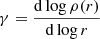 (Adhikari et al. 2014). We used simulated galaxies in IllustrisTNG to compute the average galaxy local number density ng(r) at each redshift; we then derived the logarithmic slope of nng(r), γng(r), and smoothed it with a Savitzky-Golay filter (Savitzky & Golay 1964) with an 11 bin window and a fourth order polynomial. The minimum of the resulting function is
  .
.
We checked the stability of the results by considering filters with polynomials of order two to six and fixed 11 bin windows. All of the corresponding  s are within ∼5% of
  s resulting from the fourth order polynomial; furthermore, χ2 yields very similar results for all filter choices.
Figure 4 shows γng(r) based on the average galaxy local number density profile of the 282 TNG300-1 clusters with M200c > 1014 M⊙ at z = 0.01. The orange vertical line shows the minimum of γng(r),  , an observationally accessible proxy of Rspl.
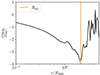 |
Fig. 4. Splashback radius from ng. The curve shows the smoothed logarithmic slope of the average local galaxy number density of the 282 clusters at z = 0.01. The orange vertical line shows the minimum, |

The black dotted curve in the upper panel of Fig. 5 shows the dependence of  on redshift. The gray shadowed area shows the standard deviation based on bootstrap resampling. Over the redshift range we sample,
  decreases by ∼38%. At fixed mass Rspl should decrease with redshift (see Sect. 1). The uncertainty increases with increasing redshift. At higher redshift, the size of the cluster sample is small (see Table 3); hence the γng(r) profile is very noisy. Locating the minima of these noisy γng(r)’s is challenging and the uncertainty is correspondingly large.
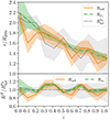 |
Fig. 5. Dynamical radii from cluster galaxy velocity in the splashback region. Upper panel: The solid orange, dash-dotted green, and dotted black lines show Rinfl, Rσv, and |


The  we derived are consistent with recent results of O’Neil et al. (2021) who also computed
  with TNG300-1. O’Neil et al. (2021) expressed their
  s in units of R200 m. We thus rescaled our
  s by computing the R200 m of the average matter density profiles. The ratio R200 m/R200c is in the range 1.63 − 1.65 throughout the redshift range and is redshift independent. We thus rescaled
  s with the average ratio R200 m/R200c = 1.64.
The  s we derived agree with those of O’Neil et al. (2021) at z ≤ 0.62; they are ∼20 − 50% larger at higher redshifts. However, the samples we extracted are not fully comparable with theirs: we defined galaxies as subhalos with stellar mass M⋆ > 108 M⊙ (see Sect. 2.1); they defined galaxies by selecting a total subhalo mass > 109 M⊙ and nonzero M⋆. Thus, the physical properties of the two samples may differ; the choice we made reduces the number of subhalos labelled as galaxies leading to poorer statistics1. The redshift dependence of
  s we obtained is consistent with previous results based on N-body simulations (More et al. 2015; Diemer 2020; O’Neil et al. 2021), although with a higher normalization.
The average galaxy radial velocity profile based on IllustrisTNG provides a route to define two new radii which closely approximate  , thus providing additional physical insight into galaxy dynamics at Rspl. We first explored a radius based on the inflection point in the radial velocity profile, Rinfl. We then turned to a radius based on a comparison between the velocity dispersion and the mean radial velocity, Rσv. In both cases these radii mark the limiting cluster-centric radius where infall no longer dominates the cluster dynamics.
The radial velocity profiles (Fig. 2) turn from concave  to convex
  as the cluster-centric radius increases. The inflection point where the change occurs, Rinfl, lies between R200c and Rvmin. The radius of the inflection point is in the range ∼(1 − 2)R200c depending on redshift (see Sect. 3.2) and is evident at every redshift. Statistically, galaxies within the inflection point cannot escape to larger radii. Thus the inflection point of vrad(r) is a dynamically motivated radius that should approximate Rspl.
Computationally, the radius corresponding to the inflection is the minimum of  . Here vrad(r) < 0. The radial velocity also increases in absolute value as the cluster-centric distance increases. Thus, at the inflection point, the local spatial change of vrad(r) is a maximum in absolute value.
To measure Rinfl, we first computed  at each redshift from the smoothed average galaxy radial velocity profile. The colored curves in Fig. 6 show the resulting
  profiles for the four redshifts listed in the legend. At each redshift, the minimum of the corresponding profile locates Rinfl. The dotted vertical lines in Fig. 6 indicate the minimum Rinfl for the correspondingly coloured curves.
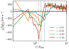 |
Fig. 6. Radial derivative of the smoothed vrad(r), and Rinfl. The blue, orange, green, and red curves show the smoothed |

For comparison with other dynamical radii, the orange vertical lines in Fig. 2 show the inflection point Rinfl at the three redshifts z = 0.01, 0.62, and 1.04, from left to right, respectively. The orange curve in Fig. 3 summarizes the behavior of Rinfl as a function of redshift. The shadowed area indicates the standard deviation based on bootstrap resampling. From z = 0.01 to z = 1.04, Rinfl decreases from ∼2.1R200c to ∼1.3R200c (∼38%). On average, Rinfl is ∼28% smaller than Rvmin.
A second radius that improves understanding of the physics within the clusters’ splashback region is Rσv, which we define from the average ratio between the 3D cluster velocity dispersion and the infall velocity, σv(r)/vrad(r). Figure 2 shows that from Rturn to Rvmin, vrad increases in absolute value from ∼0 to ∼250 − 500 km s−1 depending on the redshift. Then, from Rvmin to R200c, vrad decreases in absolute value from its maximum to ∼0. Figure 7 shows that σv(r) increases monotonically from Rturn to R200c; σv(r) increases from ∼250 − 350 km s−1 to ∼400 − 500 km s−1. At Rvmin, the ratio between σv(r) and vrad is always greater than −1: from z = 0.01 to z = 0.52 the ratio increases from ∼ − 0.97 to ∼ − 0.74; at higher redshifts, the ratio at Rvmin is ∼ − 0.72. The two profiles σv(r) and vrad always have two intersections. When σv(r) > |vrad(r)|, randomly oriented motions exceed motions aligned along the radial direction; radial motions dominate when σv(r) < |vrad(r)|. We compute Rσv by identifying the smallest cluster-centric radius where σv(r)/vrad(r) = − 1. Within this radius galaxies orbiting in the cluster potential dominate the dynamics.
 |
Fig. 7. Average galaxy velocity dispersion as a function of cluster-centric radius. The blue, orange, green, and red solid curves show the dispersion at four redshifts z = 0.01, 0.31, 0.62, and 1.04, respectively. The dashed curves show the smoothing of the correspondingly colored solid curves. |
At each redshift, we computed the average galaxy velocity dispersion profile σv(r) with an approach similar to the computation of the average vrad(r) profiles (Sect. 2.2). We considered 100 shells with linearly spaced boundaries covering the range (0 − 10)R200c. For each cluster, we computed the standard deviation of the velocities of all the galaxies inside that shell, the estimator of the velocity dispersion for the shell. In bin n for the shell with radial range (rn − rn + 1), the velocity dispersion is the square root of
 (2)
(2)
where k runs over the three spatial components,  is the mean of the k spatial component of the velocity of galaxies in bin n, and N is the number of galaxies. The single average galaxy σv(r) profile at each redshift is the mean of the velocity dispersions for the individual clusters in each bin.
The curves in Fig. 7 show the average σv(r) for clusters at the four redshifts listed in the legend within the radial range (1 − 4)R200c. Generally, σv(r) deceases with increasing cluster-centric radius. The σv(r) profile at fixed cluster-centric radius increases with redshift by ∼40% from z = 0.01 to z = 1.04. Figure 8 shows the ratio σv(r)/vrad(r) for the four redshifts listed in the legend. As in Fig. 7, we limit the radial range to (1 − 4)R200c.
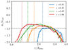 |
Fig. 8. Average ratio between the galaxy velocity dispersion and the galaxy radial velocity, as a function of cluster-centric radius. The blue, orange, green, and red solid curves show the ratio at four redshifts z = 0.01, 0.31, 0.62, and 1.04, respectively. The dashed curves show the smoothed correspondingly colored solid curves. The horizontal dash-dotted line shows σv/vrad = −1. The vertical dotted lines show Rσv corresponding to σv(r)/vrad(r) = − 1 from smoothed profiles. |
At cluster-centric distances ≲R200c, where the cluster is in approximate dynamical equilibrium, σv(r)/vrad(r) is ill-defined because vrad(r)∼0 (Fig. 2). At radii ∼(1 − 2)R200c, σv(r)/vrad(r) increases but remains < − 1. This behavior occurs at smaller radii with increasing redshift. In this radial range there is a net radial motion toward the cluster center, but the infall does not dominate over the internal cluster dynamics.
In the region where σv(r)/vrad(r) > − 1 (Fig. 8), radial infall dominates the dynamics. The center of this range is ≈Rvmin as expected (Sect. 3.2). Statistically, galaxies in this region have radial velocities directed toward the cluster center (Fig. 2); the radial velocities exceed the orbital velocities. At smaller cluster-centric radii, where σv(r)/vrad(r) < − 1, orbital motions dominate. Once galaxies migrate from the infall region where σv(r)/vrad(r) > − 1 into the inner cluster region where σv(r)/vrad(r) < − 1, they can generally no longer reach radii where σv(r)/vrad(r) > − 1. Thus the radius where σv(r)/vrad(r) = − 1, Rσv, provides another complementary physical view of the dynamics near the splashback radius.
Rσv is the innermost cluster-centric radius where σv(r)/vrad(r) = − 1. To locate Rσv, we used the ratio between the smoothed σv(r) and vrad(r) profiles. The dotted vertical lines in Fig. 8 show Rσv for the correspondingly colored ratios. The green dash-dotted curve in the upper panel of Fig. 5 shows that Rσv decreases with redshift. The green shadowed area indicates the error based on bootstrap resampling. From z = 0.01 to z = 1.04, Rσv decreases from ∼2.2R200c to ∼1.3R200c (∼40%).
At radii ≳3R200c, σv(r)/vrad(r) decreases. Although σv(r) is roughly constant, the magnitude of vrad(r) decreases as galaxies approach Rturn where they are just overcoming the Hubble flow and their net radial velocity is zero. Near the turnaround radius (∼(4.5 − 5)R200c, Sect. 3.1), vrad(r)∼0; σv(r)/vrad(r) then behaves erratically.
Figure 5 compares the observable proxy for the splashback radius,  , with the two radii Rinfl and Rσv. These radii, derived from the mean radial velocity profile, mark the transition from the infall region to the approximately virialized region where orbital motions dominate.
In the upper panel of Fig. 5, the solid orange, dash-dotted green, and dotted black lines show Rinfl (same as the orange line in Fig. 3), Rσv, and  , respectively, as a function of redshift. The shadowed bands show the bootstrapped error. In the bottom panel, the solid orange and dash-dotted green lines show the ratios
  and
and  , respectively. The orange, green, and grey shadowed areas show the 1σ confidence levels for Rinfl, Rσv, and
  , respectively.
Averaged over redshift, 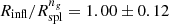 ;
; 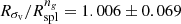 (bottom panel, Fig. 5). The redshift dependence of
  agrees with that of Rinfl and Rσv over the whole redshift range.
The radii from the velocity profile, Rinfl and Rσv, have nearly the same value as  . The dynamically derived radii are unbiased and within ∼1σ of
  . Although Rinfl and Rσv are not directly observable, they establish a connection between the splashback physics and the infall dynamics of clusters. The near equality of Rinfl, Rσv and
  suggests that Rspl corresponds to the boundary between the region where galaxies orbiting in the cluster potential dominate the dynamics and the region where infall of galaxies dominates.
4. Discussion
4.1. The cluster mass distribution
Table 3 shows that the median cluster mass generally decreases as the redshift increases because very massive systems are progressively less abundant at higher redshift. The changing distribution of cluster masses could affect the resulting dynamical radii. We explored this issue by selecting subsamples that are homogeneous.
For each redshift, we constructed homogeneous samples that include clusters with mass > M200c in the range (1.0 − 5.0)×1014 M⊙. The last column of Table 3 shows that this mass range is sampled at every redshift. A Kolmogorov–Smirnov test demonstrates that the clipped samples have indistinguishable mass distributions; the p-values are in the range (0.32 − 1.00). For each redshift, we computed the average galaxy radial velocity and the average galaxy velocity dispersion profiles for the clipped sample following Sects. 2.2 and 3.3, respectively.
The clipped Rturn are on average ∼0.1% smaller than the full sample Rturn, and they are always within ≲0.5% of the full sample values. The difference between clipped and full sample Rturn as a function of redshift is unbiased. The clipped Rvmin’s are equal to the full samples Rvmin’s at every redshift except z = 0.73 where the clipped radius exceeds the full sample radius by ∼5%.
The clipped Rinfl’s are equal to the full sample Rinfl’s at every redshift except z = 0.62 where the clipped radius exceeds the full sample radius by ∼8%. The clipped Rσv’s are on average ∼0.2% below the full sample Rσv’s and they lie within ≲0.8% of the full sample Rσv’s. Differences between the clipped and full sample Rσv’s are unbiased. The dynamical radii are all insensitive to differences among the distribution of cluster masses at different redshifts in the full samples.
4.2. Comparison of galaxy and total-matter distribution radii
Galaxies may be biased tracers of the underlying distribution of matter in the Universe, mainly comprised of dark matter (e.g., Kaiser 1984; Davis et al. 1985; White et al. 1987). IllustrisTNG enables measurement of the possible bias in the values of the dynamical radii derived from the radial velocity profiles based on galaxies by comparing them with the values derived for the total matter distribution.
We computed a single average radial velocity for the total matter distribution at each redshift with the approach of Sect. 2.2. The total matter content includes dark matter, gas, stars, and black holes, which are all included in IllustrisTNG (see Sect. 2.1). We took 200 logarithmically spaced bins (rather than the 100 we used for the velocity profile based on galaxies alone) in the radial range (0.1 − 10)R200c. The total matter distribution enables the more finely spaced bins.
At each redshift, we located the turnaround, the minimum radial velocity, and the inflection point of the average total matter radial velocity profiles (Sect. 3). The radii derived from the total mass distribution are  ,
,  , and
, and  , respectively. The red, blue, and orange lines in Fig. 9 show the ratios between the galaxy based and total matter based radii:
  ,
,  , and
, and  as a function of redshift. The horizontal dotted lines show the corresponding median ratio for the 11 redshift bins. The shadowed band of corresponding color shows the 1σ confidence range for each of the ratios.
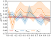 |
Fig. 9. Ratio between dynamical radii from radial velocity profiles based on galaxies and on the total matter. The red, blue, and orange lines show the ratio between the turnaround, the minimum radial velocity, and the inflection point of average radial velocity profiles of galaxies and total matter, as a function of redshift. The horizontal dotted lines show the median ratio of the corresponding curve for the 11 redshift bins. The shadowed band in each case shows the 1σ confidence range. |
The radii Rturn and Rvmin based on galaxy velocities are consistent with the radii based on the total matter velocities. Averaging over redshift, the median 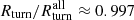 (red dotted horizontal line); Rturn is always within ≲4% of
  . On average,
 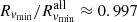 (blue dotted horizontal line), and Rvmin overestimates (underestimates)
  by ≲ + 10% (−8%) at most. The Rinfl’s based on galaxy velocities generally exceed the corresponding radii based on the total matter. Averaging over redshift,
 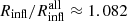 (orange dotted horizontal line), and Rinfl overestimates (underestimates)
  by ≲ + 14% (−12%). The results are consistent with equality at ∼1σ level. Figure 9 shows that the ratios are essentially independent of redshift.
The mild overestimation of Rinfl relative to  is consistent with the behaviour of Rspl found by O’Neil et al. (2021) who also analyze TNG300-1. They computed the proxy for Rspl based on galaxies,
  , and compared it with the analogous splashback radius based on all of the matter,
  . For systems with masses ≳1014 M⊙,
 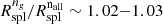 , with a considerable dispersion that allows overestimations as large as ∼15% (see their Fig. 6). For the inflection point, the average ratio over the 11 redshift bins we sampled is
 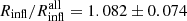 . This value is consistent with O’Neil et al. (2021) within the uncertainty. We conclude that, as O’Neil et al. (2021) show for the splashback proxy, the bias between dynamical radii based on galaxies and all of the matter is small.
5. Conclusion
Simulated galaxies drawn from the IllustrisTNG300-1 simulations (Pillepich et al. 2018; Springel et al. 2018; Nelson et al. 2019) enable exploration of the infall region of 1697 galaxy clusters with M200c > 1014 M⊙ and redshift 0.01 ≤ z ≤ 1.04 (Pizzardo et al. 2023a,b). For these systems, we revisited the classical turnaround radius Rturn that defines the outer boundary of a cluster (Gunn et al. 1972; Silk 1974; Schechter 1980) and the characteristic minimum infall velocity Rvmin (De Boni et al. 2016; Vallés-Pérez et al. 2020; Fong & Han 2021; Pizzardo et al. 2021, 2023b). Based on the galaxy radial velocity profile, vrad(r), we derived two new measures of the inner boundary of the infall region. Both of these radii lie within the radial velocity minimum and coincide with the splashback radius, Rspl (Adhikari et al. 2014; Diemer & Kravtsov 2014; More et al. 2015).
The galaxy average radial velocity profile, vrad(r), enables identification of the turnaround radius, Rturn, where galaxies decouple from the Hubble flow. The Rturn’s lie in the range (4.67 − 4.94)R200c, are insensitive to redshift, and agree with the Meiksin analytic approximation (Meiksin 1985).
The galaxy average radial velocity profile, vrad(r), has a well-defined minimum, Rvmin. The value of Rvmin decreases from 2.8R200c at z = 0.01 to 1.8R200c at z = 1.04. The maximum infall velocity itself increases with redshift.
Inside Rvmin, we developed two new dynamical radii that mark the inner boundary of the infall region: (i) Rinfl is the inflection point of vrad(r), the cluster-centric radius where the derivative of vrad(r) is maximum in absolute value, and (ii) Rσv is the smallest cluster-centric radius where σv(r) = |vrad(r)|. Outside these radii, infall dominates the cluster dynamics; within these radii orbital motions dominate over infall.
To within 1σ, the two dynamical radii, Rinfl and Rσv, coincide with  , the radius where the logarithmic derivative of the galaxy average number density profile has a minimum. This radius is an observable proxy for the splashback radius, Rspl, often determined from N-body simulations (Diemer & Kravtsov 2014; Diemer et al. 2017; Mansfield et al. 2017; Diemer 2018; Xhakaj et al. 2020). Averaged over redshift,
  , and
, and  .
.
Galaxies may be biased tracers of the total matter content of a cluster. For the set of IllustrisTNG clusters, the ratios between galaxy and total matter Rturn is 0.997 ± 0.014; the corresponding ratio for Rvmin is 0.997 ± 0.056. The radius Rinfl for galaxies exceeds the value for all matter by (8.2 ± 7.4)%. O’Neil et al. (2021) measure a similarly negligible bias between values of Rspl for galaxies and the entire matter distribution.
The consistency between the dynamical radii, Rinfl and Rσv, and the splashback radius,  , provides an enhanced physical view of
  as the inner boundary of the infall region where galaxies are infalling onto the cluster core. Currently,
  provides a direct observational route to this physical cluster boundary. In the future, observations that include accurate independent distance measures for galaxies around clusters and their filamentary structures will allow observational determination of the velocity field for infalling galaxies (Odekon et al. 2022). Some limited observations are available in the nearby Universe; they should become more broadly available at greater and greater depths in the Universe. Thus observational proxies for the dynamical radii Rinfl and Rσv should eventually complement determination of Rspl from the cluster density profile.
O’Neil et al. (2021) computed  by fitting the density profiles with an analytic function. They show that different fitting procedures can affect the splashback radius by ≲8%. The agreement between the
  s we derived and those of O’Neil et al. (2021) at z ≲ 0.62 suggests that our computation of
  is robust. Mild discrepancies at high redshift result from different sampling of the simulated galaxy population.
Acknowledgments
We thank the referee for comments that led to improvements in this paper. We thank Jubee Sohn for insightful discussions. M.P. and I.D. acknowledge the support of the Canada Research Chair Program and the Natural Sciences and Engineering Research Council of Canada (NSERC, funding reference number RGPIN-2018-05425). The Smithsonian Institution supports the research of M.J.G. and S.J.K. Part of the analysis was performed with the computer resources of INFN in Torino and of the University of Torino. This research has made use of NASA’s Astrophysics Data System Bibliographic Services. All of the primary TNG simulations have been run on the Cray XC40 Hazel Hen supercomputer at the High Performance Computing Center Stuttgart (HLRS) in Germany. They have been made possible by the Gauss Centre for Supercomputing (GCS) large-scale project proposals GCS-ILLU and GCS-DWAR. GCS is the alliance of the three national supercomputing centres HLRS (Universitaet Stuttgart), JSC (Forschungszentrum Julich), and LRZ (Bayerische Akademie der Wissenschaften), funded by the German Federal Ministry of Education and Research (BMBF) and the German State Ministries for Research of Baden-Wuerttemberg (MWK), Bayern (StMWFK) and Nordrhein-Westfalen (MIWF). Further simulations were run on the Hydra and Draco supercomputers at the Max Planck Computing and Data Facility (MPCDF, formerly known as RZG) in Garching near Munich, in addition to the Magny system at HITS in Heidelberg. Additional computations were carried out on the Odyssey2 system supported by the FAS Division of Science, Research Computing Group at Harvard University, and the Stampede supercomputer at the Texas Advanced Computing Center through the XSEDE project AST140063.
References
- Achitouv, I., Wagner, C., Weller, J., & Rasera, Y. 2014, J. Cosmol. Astropart. Phys., 2014, 077 [CrossRef] [Google Scholar]
- Adhikari, S., Dalal, N., & Chamberlain, R. T. 2014, JCAP, 11, 019 [Google Scholar]
- Adhikari, S., Shin, T.-H., Jain, B., et al. 2021, ApJ, 923, 37 [NASA ADS] [CrossRef] [Google Scholar]
- Baxter, E., Chang, C., Jain, B., et al. 2017, ApJ, 841, 18 [NASA ADS] [CrossRef] [Google Scholar]
- Baxter, E. J., Adhikari, S., Vega-Ferrero, J., et al. 2021, MNRAS, 508, 1777 [NASA ADS] [CrossRef] [Google Scholar]
- Bertschinger, E. 1985, ApJS, 58, 39 [Google Scholar]
- Bianconi, M., Buscicchio, R., Smith, G. P., et al. 2021, ApJ, 911, 136 [Google Scholar]
- Bower, R. G. 1991, MNRAS, 248, 332 [NASA ADS] [CrossRef] [Google Scholar]
- Chang, C., Baxter, E., Jain, B., et al. 2018, ApJ, 864, 83 [NASA ADS] [CrossRef] [Google Scholar]
- Corasaniti, P. S., & Achitouv, I. 2011, Phys. Rev. Lett., 106, 241302 [NASA ADS] [CrossRef] [Google Scholar]
- Cornwell, D. J., Kuchner, U., Aragón-Salamanca, A., et al. 2022, MNRAS, 517, 1678 [NASA ADS] [CrossRef] [Google Scholar]
- Cornwell, D. J., Aragón-Salamanca, A., Kuchner, U., et al. 2023, MNRAS, 524, 2148 [NASA ADS] [CrossRef] [Google Scholar]
- Cuesta, A. J., Prada, F., Klypin, A., & Moles, M. 2008, MNRAS, 389, 385 [NASA ADS] [CrossRef] [Google Scholar]
- Cupani, G., Mezzetti, M., & Mardirossian, F. 2008, MNRAS, 390, 645 [NASA ADS] [CrossRef] [Google Scholar]
- Cupani, G., Mezzetti, M., & Mardirossian, F. 2011, MNRAS, 417, 2554 [NASA ADS] [CrossRef] [Google Scholar]
- Dacunha, T., Belyakov, M., Adhikari, S., et al. 2022, MNRAS, 512, 4378 [NASA ADS] [CrossRef] [Google Scholar]
- Davis, M., Efstathiou, G., Frenk, C. S., & White, S. D. M. 1985, ApJ, 292, 371 [Google Scholar]
- Deason, A. J., Oman, K. A., Fattahi, A., et al. 2021, MNRAS, 500, 4181 [Google Scholar]
- De Boni, C., Serra, A. L., Diaferio, A., Giocoli, C., & Baldi, M. 2016, ApJ, 818, 188 [NASA ADS] [CrossRef] [Google Scholar]
- De Simone, A., Maggiore, M., & Riotto, A. 2011, MNRAS, 418, 2403 [CrossRef] [Google Scholar]
- Diaferio, A. 1999, MNRAS, 309, 610 [CrossRef] [Google Scholar]
- Diaferio, A., & Geller, M. J. 1997, ApJ, 481, 633 [NASA ADS] [CrossRef] [Google Scholar]
- Diemer, B. 2017, ApJS, 231, 5 [NASA ADS] [CrossRef] [Google Scholar]
- Diemer, B. 2018, ApJS, 239, 35 [NASA ADS] [CrossRef] [Google Scholar]
- Diemer, B. 2020, ApJ, 903, 87 [NASA ADS] [CrossRef] [Google Scholar]
- Diemer, B., & Kravtsov, A. V. 2014, ApJ, 789, 1 [NASA ADS] [CrossRef] [Google Scholar]
- Diemer, B., Mansfield, P., Kravtsov, A. V., & More, S. 2017, ApJ, 843, 140 [NASA ADS] [CrossRef] [Google Scholar]
- Fong, M., & Han, J. 2021, MNRAS, 503, 4250 [NASA ADS] [CrossRef] [Google Scholar]
- Gao, H., Han, J., Fong, M., Jing, Y. P., & Li, Z. 2023, ApJ, 953, 37 [NASA ADS] [CrossRef] [Google Scholar]
- Geller, M. J., Diaferio, A., & Kurtz, M. J. 1999, ApJ, 517, L23 [NASA ADS] [CrossRef] [Google Scholar]
- Gonzalez, A. H., George, T., Connor, T., et al. 2021, MNRAS, 507, 963 [NASA ADS] [CrossRef] [Google Scholar]
- Gunn, J. E., Gott, J., & Richard, I. 1972, ApJ, 176, 1 [Google Scholar]
- Ivezić, Ž., Kahn, S. M., Tyson, J. A., et al. 2019, ApJ, 873, 111 [Google Scholar]
- Kaiser, N. 1984, ApJ, 284, L9 [NASA ADS] [CrossRef] [Google Scholar]
- Lacey, C., & Cole, S. 1993, MNRAS, 262, 627 [NASA ADS] [CrossRef] [Google Scholar]
- Lahav, O., Lilje, P. B., Primack, J. R., & Rees, M. J. 1991, MNRAS, 251, 128 [Google Scholar]
- Mansfield, P., Kravtsov, A. V., & Diemer, B. 2017, ApJ, 841, 34 [NASA ADS] [CrossRef] [Google Scholar]
- Marshall, J., Bolton, A., Bullock, J., et al. 2019, BAAS, 51, 126 [Google Scholar]
- More, S., Diemer, B., & Kravtsov, A. V. 2015, ApJ, 810, 36 [Google Scholar]
- More, S., Miyatake, H., Takada, M., et al. 2016, ApJ, 825, 39 [NASA ADS] [CrossRef] [Google Scholar]
- Murata, R., Sunayama, T., Oguri, M., et al. 2020, PASJ, 72, 64 [NASA ADS] [CrossRef] [Google Scholar]
- Musso, M., Cadiou, C., Pichon, C., et al. 2018, MNRAS, 476, 4877 [Google Scholar]
- Nelson, D., Springel, V., Pillepich, A., et al. 2019, Comput. Astrophys. Cosmol., 6, 1 [NASA ADS] [CrossRef] [Google Scholar]
- Odekon, M. C., Jones, M. G., Graham, L., Kelley-Derzon, J., & Halstead, E. 2022, ApJ, 935, 130 [NASA ADS] [CrossRef] [Google Scholar]
- O’Neil, S., Barnes, D. J., Vogelsberger, M., & Diemer, B. 2021, MNRAS, 504, 4649 [CrossRef] [Google Scholar]
- O’Neil, S., Borrow, J., Vogelsberger, M., & Diemer, B. 2022, MNRAS, 513, 835 [CrossRef] [Google Scholar]
- Peebles, P. J. E. 1980, The Large-scale Structure of the Universe (Princeton University Press) [Google Scholar]
- Pillepich, A., Springel, V., Nelson, D., et al. 2018, MNRAS, 473, 4077 [Google Scholar]
- Pizzardo, M., Di Gioia, S., Diaferio, A., et al. 2021, A&A, 646, A105 [NASA ADS] [CrossRef] [EDP Sciences] [Google Scholar]
- Pizzardo, M., Geller, M. J., Kenyon, S. J., Damjanov, I., & Diaferio, A. 2023a, A&A, 675, A56 [NASA ADS] [CrossRef] [EDP Sciences] [Google Scholar]
- Pizzardo, M., Geller, M. J., Kenyon, S. J., Damjanov, I., & Diaferio, A. 2023b, A&A, 680, A48 [NASA ADS] [CrossRef] [EDP Sciences] [Google Scholar]
- Press, W. H., & Schechter, P. 1974, ApJ, 187, 425 [Google Scholar]
- Regos, E., & Geller, M. J. 1989, AJ, 98, 755 [NASA ADS] [CrossRef] [Google Scholar]
- Rines, K., & Diaferio, A. 2006, AJ, 132, 1275 [Google Scholar]
- Rines, K., Geller, M. J., Diaferio, A., & Kurtz, M. J. 2013, ApJ, 767, 15 [NASA ADS] [CrossRef] [Google Scholar]
- Savitzky, A., & Golay, M. 1964, J. Anal. Chem., 36, 1627 [Google Scholar]
- Schechter, P. L. 1980, AJ, 85, 801 [NASA ADS] [CrossRef] [Google Scholar]
- Serra, A. L., Diaferio, A., Murante, G., & Borgani, S. 2011, MNRAS, 412, 800 [NASA ADS] [Google Scholar]
- Sheth, R. K., & Tormen, G. 2002, MNRAS, 329, 61 [Google Scholar]
- Shin, T., Adhikari, S., Baxter, E. J., et al. 2019, MNRAS, 487, 2900 [NASA ADS] [CrossRef] [Google Scholar]
- Silk, J. 1974, ApJ, 193, 525 [NASA ADS] [CrossRef] [Google Scholar]
- Springel, V., Pakmor, R., Pillepich, A., et al. 2018, MNRAS, 475, 676 [Google Scholar]
- Springel, V., White, S. D. M., Tormen, G., & Kauffmann, G. 2001, MNRAS, 328, 726 [Google Scholar]
- Tamura, N., Takato, N., Shimono, A., et al. 2016, SPIE, 9908, 99081M [NASA ADS] [Google Scholar]
- Umetsu, K., Medezinski, E., Nonino, M., et al. 2014, ApJ, 795, 163 [NASA ADS] [CrossRef] [Google Scholar]
- Umetsu, K., Zitrin, A., Gruen, D., et al. 2016, ApJ, 821, 116 [Google Scholar]
- Umetsu, K., Sereno, M., Lieu, M., et al. 2020, ApJ, 890, 148 [NASA ADS] [CrossRef] [Google Scholar]
- Vallés-Pérez, D., Planelles, S., & Quilis, V. 2020, MNRAS, 499, 2303 [CrossRef] [Google Scholar]
- Villumsen, J. V., & Davis, M. 1986, ApJ, 308, 499 [NASA ADS] [CrossRef] [Google Scholar]
- White, S. D. M., Davis, M., Efstathiou, G., & Frenk, C. S. 1987, Nature, 330, 451 [NASA ADS] [CrossRef] [Google Scholar]
- White, S. D. M., & Rees, M. J. 1978, MNRAS, 183, 341 [Google Scholar]
- Xhakaj, E., Diemer, B., Leauthaud, A., et al. 2020, MNRAS, 499, 3534 [NASA ADS] [CrossRef] [Google Scholar]
- Zhang, J., Ma, C.-P., & Fakhouri, O. 2008, MNRAS, 387, L13 [CrossRef] [Google Scholar]
- Zürcher, D., & More, S. 2019, ApJ, 874, 184 [CrossRef] [Google Scholar]
All Tables
All Figures
|
Fig. 1. Relation between M200c and comoving R200c for IllustrisTNG clusters. Left panel: Blue, orange, green, and red points show the M200c − R200c relation for clusters in four redshift bins z = 0.01, 0.31, 0.62, and z = 1.04, respectively. Colored squares with error bars show the median and interquartile range in each redshift bin. Right panel: Mass distribution histograms, with areas normalized to unity. |
| In the text | |
|
Fig. 2. Average radial velocity profiles and dynamical radii. Solid curves show the average galaxy radial velocity profiles of clusters at three redshifts: z = 0.01, 0.62, and 1.04, from left to right, respectively. Dashed curves show the Savitzky–Golay (Savitzky & Golay 1964) smoothed profiles. Shaded bands show the error in the smoothed profiles. In each panel, the red, blue, and orange lines show the turnaround, the minimum radial velocity, and the inflection point radii, respectively, derived from the average radial velocity profiles (see Sect. 3). |
| In the text | |
|
Fig. 3. Dynamical radii from smoothed average galaxy radial velocity profiles. The red, blue, and orange lines show the mass averaged turnaround radius (Sect. 3.1), the point of minimum vrad(r) (Sect. 3.2), and the inflection point of vrad(r) (Sect. 3.3), as a function of redshift, respectively. Shadowed bands show the error from bootstrap resampling of the correspondingly colored radius. |
| In the text | |
|
Fig. 4. Splashback radius from ng. The curve shows the smoothed logarithmic slope of the average local galaxy number density of the 282 clusters at z = 0.01. The orange vertical line shows the minimum, |
| In the text | |
|
Fig. 5. Dynamical radii from cluster galaxy velocity in the splashback region. Upper panel: The solid orange, dash-dotted green, and dotted black lines show Rinfl, Rσv, and |
| In the text | |
|
Fig. 6. Radial derivative of the smoothed vrad(r), and Rinfl. The blue, orange, green, and red curves show the smoothed |
| In the text | |
|
Fig. 7. Average galaxy velocity dispersion as a function of cluster-centric radius. The blue, orange, green, and red solid curves show the dispersion at four redshifts z = 0.01, 0.31, 0.62, and 1.04, respectively. The dashed curves show the smoothing of the correspondingly colored solid curves. |
| In the text | |
|
Fig. 8. Average ratio between the galaxy velocity dispersion and the galaxy radial velocity, as a function of cluster-centric radius. The blue, orange, green, and red solid curves show the ratio at four redshifts z = 0.01, 0.31, 0.62, and 1.04, respectively. The dashed curves show the smoothed correspondingly colored solid curves. The horizontal dash-dotted line shows σv/vrad = −1. The vertical dotted lines show Rσv corresponding to σv(r)/vrad(r) = − 1 from smoothed profiles. |
| In the text | |
|
Fig. 9. Ratio between dynamical radii from radial velocity profiles based on galaxies and on the total matter. The red, blue, and orange lines show the ratio between the turnaround, the minimum radial velocity, and the inflection point of average radial velocity profiles of galaxies and total matter, as a function of redshift. The horizontal dotted lines show the median ratio of the corresponding curve for the 11 redshift bins. The shadowed band in each case shows the 1σ confidence range. |
| In the text | |
Current usage metrics show cumulative count of Article Views (full-text article views including HTML views, PDF and ePub downloads, according to the available data) and Abstracts Views on Vision4Press platform.
Data correspond to usage on the plateform after 2015. The current usage metrics is available 48-96 hours after online publication and is updated daily on week days.
Initial download of the metrics may take a while.