| Issue |
A&A
Volume 696, April 2025
|
|
|---|---|---|
| Article Number | A27 | |
| Number of page(s) | 17 | |
| Section | Planets, planetary systems, and small bodies | |
| DOI | https://doi.org/10.1051/0004-6361/202347510 | |
| Published online | 01 April 2025 | |
The CARMENES search for exoplanets around M dwarfs
Understanding the wavelength dependence of radial velocity measurements
1
Thüringer Landessternwarte Tautenburg,
Sternwarte 5,
07778
Tautenburg,
Germany
2
School of Physical Sciences, The Open University,
Walton Hall,
Milton Keynes
MK7 6AA,
UK
3
Instituto de Astrofísica de Andalucía (CSIC), Glorieta de la Astronomía s/n,
18008
Granada,
Spain
4
Landessternwarte, Zentrum für Astronomie der Universität Heidelberg,
Königstuhl 12,
69117
Heidelberg,
Germany
5
Instituto de Astrofísica de Canarias, c/ Vía Láctea s/n,
38205
La Laguna, Tenerife,
Spain
6
Departamento de Astrofísica, Universidad de La Laguna,
38206
Tenerife,
Spain
7
Institut für Astrophysik and Geophysik, Georg-August-Universität,
Friedrich-Hund-Platz 1,
37077
Göttingen,
Germany
8
Centre for Planetary Habitability, Department of Geosciences, University of Oslo,
Sem Saelands vei 2b,
0315
Oslo,
Norway
9
Centro de Astrobiología (CSIC-INTA), ESAC, Camino Bajo del Castillo s/n,
28692
Villanueva de la Cañada, Madrid,
Spain
10
Hamburger Sternwarte, Universität Hamburg,
Gojenbergsweg 112,
21029
Hamburg,
Germany
11
Institut de Ciències de l’Espai (CSIC), Campus UAB, c/ de Can Magrans s/n,
08193
Bellaterra, Barcelona,
Spain
12
Institut d’Estudis Espacials de Catalunya,
08034
Barcelona,
Spain
13
Centro Astronómico Hispano en Andalucía (CAHA), Observatorio de Calar Alto, Sierra de los Filabres,
04550
Gérgal, Almería,
Spain
14
Department of Physics, University of Warwick,
Gibbet Hill Road,
Coventry
CV4 7AL,
UK
15
Centre for Exoplanets and Habitability, University of Warwick,
Coventry
CV4 7AL,
UK
16
Max-Planck-Institut für Astronomie,
Königstuhl 17,
69117
Heidelberg,
Germany
17
Fakultät für Physik, Universitäts-Sternwarte, Ludwig-Maximilians-Universität München,
Scheinerstr. 1,
81679
München,
Germany
18
Facultad de Ciencias Físicas, Departamento de Física de la Tierra y Astrofísica & IPARCOS-UCM (Instituto de Física de Partículas y del Cosmos de la UCM), Universidad Complutense de Madrid,
28040
Madrid,
Spain
★ Corresponding author; sandrajeffers.astro@gmail.com
Received:
20
July
2023
Accepted:
20
October
2024
Context. Current exoplanet surveys are focused on detecting small exoplanets orbiting in the liquid-water habitable zones of their host stars. Despite recent significant advancements in instrumentation, the main limitation in detecting these exoplanets is the intrinsic variability of the host star itself.
Aims. Our aim is to investigate the wavelength dependence of high-precision radial velocities (RV), as stellar activity induced RVs should exhibit a wavelength dependence while the RV variation due to an orbiting planet will be wavelength independent.
Methods. We used the chromatic index (CRX) to quantify the slope of the measured RVs as a function of logarithmic wavelength of the full CARMENES guaranteed time observations (GTO) data set spanning more than eight years of observations of over 350 stars. We investigated the dependence of the CRX in the full Carmenes GTO sample on 24 stellar activity indices in the visible and near-infrared channels of the CARMENES spectrograph and each star’s stellar parameters. We also present an updated convective turnover time scaling for the calculation of the stellar Rossby number for M dwarfs.
Results. Our results show that approximately 17% of GTO stars show a strong or a moderate correlation between the CRX and RV. We can improve the measured RVs by a factor of up to nearly 4 in terms of the root mean square (rms) by subtracting the RV predicted by the CRX-RV correlation from the measured RVs. Mid-M dwarfs with moderate rotational velocities and moderate CRX-gradients, with quasi-stable activity features, have the best rms improvement factors.
Conclusions. We conclude that the CRX is a powerful diagnostic in mitigation of stellar activity and the search for low mass rocky planets.
Key words: techniques: radial velocities / planets and satellites: detection / stars: activity / stars: low-mass / stars: magnetic field / starspots
© The Authors 2025
 Open Access article, published by EDP Sciences, under the terms of the Creative Commons Attribution License (https://creativecommons.org/licenses/by/4.0), which permits unrestricted use, distribution, and reproduction in any medium, provided the original work is properly cited.
This article is published in open access under the Subscribe to Open model. Subscribe to A&A to support open access publication.
1 Introduction
In recent years, we have seen exceptional progress in the area of wavelength calibration and the development of high-precision, highly stable instrumentation using the RV technique and aimed at detecting small rocky exoplanets orbiting in the liquid-water habitable zones of their host stars. These include ESPRESSO (Pepe et al. 2021), EXPRES (Jurgenson et al. 2016), and MAROON-X (Bean 2020), among others, with tens of cm s−1 precision. Recently, Suárez Mascareño et al. (2020) reported the achievement of a precision of 30 cm s−1 for ESPRESSO observations of Proxima Centauri. The current limitation in detecting small rocky planets is not instrumental capability, but the intrinsic variability of the host stars themselves (see recent works e.g. Crass et al. 2021; Zhao et al. 2022, and references therein).
All stars with masses just above and lower than the Sun possess an internal convection zone and exhibit some degree of magnetic activity from very low (e.g. the early-M dwarf GJ 887: Jeffers et al. 2020) to very high (e.g. the early and mid M dwarfs AU Mic and EV Lac: Cale et al. 2021; Klein et al. 2022; Jeffers et al. 2022; Bellotti et al. 2022). The presence of this activity induces an asymmetry in the shape of the stellar photospheric absorption lines which limits our ability to determine the star’s centre-of-mass motion via the position of the line’s centre (Dravins et al. 1981; Saar & Donahue 1997; Lagrange et al. 2010; Meunier et al. 2010; Reiners et al. 2010; Barnes et al. 2011; Dumusque et al. 2014; Haywood et al. 2014). This consequently results in an additional activity-induced RV contribution which impacts the detection and the measurement of the masses of small planets orbiting close to their host stars. There are also a large number of methods that have been developed to remove the activity-induced component to the RVs. However, from the extensive testing of different activity-removal methods by Zhao et al. (2022), they conclude that no method is successful in routinely achieving a reduction in the RV root mean square (rms) to sub-meter-per-second levels.
In this work, we aim to understand the wavelength-dependent activity diagnostics of the full data set secured as part of the Calar Alto high-Resolution search for M dwarfs with Exoearths with Near-infrared and optical Echelle Spectrographs (CARMENES; Quirrenbach et al. (2018, 2020)) guaranteed time observations (GTO) survey. The CARMENES GTO sample was selected to contain the brightest stars in the J band for each M dwarf sub-spectral type bin that are observable from Calar Alto Observatory in southern Spain and have no stellar companion within 5 arcsec. This selection procedure for the GTO sample has ensured that it includes both magnetically active and inactive stars. Now, after over 8 years of operation and with more than 20000 spectra in hand (Ribas et al. 2023), we have a statistically significant sample that we can use to improve our understanding of the impact of stellar activity on high-precision RV measurements. One important diagnostic parameter in the search for exoplanets orbiting stars displaying stellar activity is an analysis of the wavelength dependence of the measured RV values. This is because the features of stellar activity, such as dark cool starspots, are typically wavelength-dependent because the contrast between starspots and the stellar photosphere is smaller at longer wavelengths. In contrast, the RV signal from an orbiting exoplanet is independent of wavelength.
The chromatic index (CRX) is a measure of the RV variation as a function of wavelength. It is defined by taking the slope of the RVs in every spectral order as a function of logarithmic wavelength (Zechmeister et al. 2018). The CRX-index has been shown by Jeffers et al. (2022), using a low-resolution Dopplerimaging technique, to be directly correlated with starspot coverage for the mid M-dwarf EV Lac. This is consistent with (i) the simulations of Baroch et al. (2020), who combined the CRXindex with photometric observations of YZ CMi to constrain the spot-filling factor and YZ CMi’s spot and photosphere temperature contrast and (ii) the previous work of Tal-Or et al. (2018), who investigated the CRX-index for only the most active stars in the CARMENES GTO sample using the first 1.5 years of CARMENES data. More recently, Lafarga et al. (2020) investigated periodicities found in RVs and nine activity indicators in the CARMENES GTO sample. They concluded that the CRX is as efficient as the line bisector (Queloz et al. 2001) as indicator of activity for active M dwarfs. Other recent work by Collier Cameron et al. (2021) (and also Lisogorskyi et al. 2019) has exploited the wavelength dependence of RV induced by stellar activity to separate RVs with dynamical origin from stellar activity induced variability.
In this paper, we aim to empirically understand the wavelength variations of RVs using the CRX-index and to quantify how to remove this contribution from the RVs. In Sect. 2, we define the CRX-index. In Sect. 3, we describe the observations and define how the CRX stars were selected from the full CARMENES GTO sample. In Sect. 4, we investigate the dependence of CRX-index on fundamental stellar parameters. In Sect. 5, we use the wavelength information contained in the CRX-index to remove stellar activity from the RVs. We discuss the implications of our results in Sect. 6.
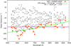 |
Fig. 1 Illustration of the RV variation with wavelength, where the central wavelength is given for each order. Shown are the same data as in Fig. 2, with the steepest positive slope shown by red points. The green line indicates the slope of these points, which is the CRX-index for each individual spectrum. The weighted RV measurement is shown by the purple line. The wavelength spacing is logarithmic. |
2 CRX: dependence of RVs with wavelength
2.1 Definition of the CRX
The CRX-index is defined as the slope of the RV as a function of logarithmic wavelength (Zechmeister et al. 2018) for each spectrum. The RV of each spectrum is computed using weighted averages to account for the wavelength dependence of the RVs (more details in Sect. 3.1). This is illustrated in Fig. 1, which shows the wavelength dependent RVs of 10 spectra of the mid-M dwarf EV Lac. The spectrum exhibiting the steepest positive gradient is illustrated with red points and a linear fit in green. The RV value computed by serval is shown as a horizontal purple line.
Figure 2 shows the CRX calculation in more detail for the same 10 spectra that are illustrated in Fig. 1. Because the spectra span less than two complete rotations of EV Lac (Prot = 4.349 d; Jeffers et al. 2022), the effects of evolution due to stellar activity should be minimal. Each spectrum is coloured according to the stellar rotation phase. The CRX-index measured for each of the spectra in Fig. 2 (top left panel) is shown as a function of RV in Fig. 2 (top-right panel), where the colour coding is the same in both panels.
The gradient of the CRX-index versus RV distribution for a series of spectra is referred to as the CRX-gradient in the work that follows. For each star, we define the CRX-length as RVmax−RVmin, where the RVmin and the RVmax are the minimum and maximum RV values from all of the available spectra (using 90 and 10 percentiles). We prefer this definition since CRX variation (CRXmax to CRXmin) and CRX are directly related, while CRX-length is most readily calculated directly from the RVs, even in the absence of CRX-index measurements. The large variations in the CRX-index as a function of rotation phase (as illustrated in Fig. 2) demonstrate how the CRX-index evolves over the stellar rotation period due to the presence of activity features on the stellar surface. The CRX-index for each individual spectrum, and consequently the CRX-gradient for a series of spectra, has been directly linked to the distribution of dark starspots on the stellar surface using low resolution Doppler imaging techniques by Jeffers et al. (2022). The lower two panels of Fig. 2 show the variation of CRX-index and RV as a function of stellar rotational phase, with the same colouring as in the upper panels.
The data shown in Fig. 2 are for the VIS channel only as the errors in the NIR channel are too high for meaningful interpretation for the case of EV Lac. Even though the NIR data are not shown, we do not expect to see a convergence of the slopes at longer wavelengths as is suggested by the outer edges of the light grey region in Fig. 2 (top-left panel). As discussed by Jeffers et al. (2022), a black-body scaling of the spot and photospheric flux ratios will remain constant continuing to NIR wavelengths, in agreement with PHOENIX models for the spot and photosphere ratio. A more detailed description of the full data set of EV Lac was previously presented by Jeffers et al. (2022).
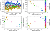 |
Fig. 2 Illustration of the behaviour of the CARMENES visible channel CRX for the mid-M dwarf EV Lac. Top-left: variation of RV as a function of wavelength (spacing is logarithmic). The CRX-index is the slope of RV vs log(λ) for each spectrum. A total of 10 CARMENES spectra are shown covering approximately one stellar rotation. The upper and lower boundaries are the fits to the most positive and negative RV values. Top right: The CRX-gradient, illustrating the CRX-index as a function of the ‘mean’ RV. Bottom-left and bottom-right: CRX vs. rotation phase and RV vs rotation phase illustrating the anti-correlation of CRX-index (i.e. the negative CRX-gradient shown in the top right panel). The plotted points in each panel are colour coded according to stellar rotation phase. |
2.2 Comparison of the CRX with different instruments
The CRX will exhibit a different behaviour when investigated with different spectrographs with varying wavelength coverage and spectral resolution. The comparison of the CRX between data secured with HARPS and CARMENES has been previously investigated by Zechmeister et al. (2018) for the stars YZ CMi, and GJ 3379, and Kossakowski et al. (2022) for AD Leo. In general, the CRX shows a negative slope for both HARPS and CARMENES datasets of YZ CMi while for GJ 3379, only the CARMENES data show a significant chromatic variation. Similarly, CARMENES M dwarf K2-18 has been reported by Radica et al. (2022) to show chromatic behaviour at a level that is below our threshold of Pearson’s r > 0.5. Similar to GJ 3379, this is not visible in the HARPS dataset of K2-18. Surprisingly, the CRX of AD Leo shows a positive slope for archival HARPS data and a negative slope for CARMENES data (Kossakowski et al. 2022; Zechmeister et al. 2018) and significantly lower amplitude for much redder wavelengths (Carmona et al. 2023). The comparison of chromaticity of RVs across a very broad wavelength regimes has the potential to give a crucial insight into the activity of these stars. However, simultaneous observations across a broad wavelength range are required to truly compare the wavelength dependence, as features of stellar activity can evolve on timescales of a few stellar rotation periods.
2.3 Modelling the CRX
The effect of dark starspots on the wavelength dependence of RVs has previously been investigated by Desort et al. (2007); Barnes et al. (2011); Collier Cameron et al. (2021), among many others. In particular, the CRX has been simulated by Baroch et al. (2020) using spectroscopic and photometric data for the mid-M dwarf YZ CMi. They demonstrated that the CRX-index, computed for each spectrum, can be used to determine and break the degeneracy between the spot-filling factor and temperature contrast between the starspot and unspotted photosphere.
Recent works have shown that the CRX-index versus RV relation can have an inclined lemniscate (∞) or figure-of-eight shape, with a typically negative slope, which results from a slight phase offset between the phase curves of the RVs and the CRX values (examples include Baroch et al. 2020; Jeffers et al. 2022, for YZ CMi and EV Lac respectively). This is comparable to the inclined-lemniscate shape established for RV versus bisector inverse slope (BIS) relations for co-rotating cool spots (Desort et al. 2007; Saar & Donahue 1997; Boisse et al. 2011). For the BIS, Boisse et al. (2011) attribute this to result from foreshortening and limb-darkening effects, while for the CRX, Baroch et al. (2020) considered that the offset results from the combined effects of limb darkening and convective blue shift. The example of the CRX-index versus RV relation (shown in Fig. 2) for the mid-M dwarf EV Lac is almost a straight line due to the dominance of high-latitude spot features (see the surface brightness maps reconstructed by Jeffers et al. 2022) and to the limited time sampling of the data, which covers only a few rotation periods. We would expect a higher amplitude lemniscate shape if there were a higher degree of spot coverage located at equatorial latitudes as has been modelled for the BIS (Boisse et al. 2011).
Empirical data used to derive spot-to-photospheric temperature contrasts using the Doppler imaging technique.
2.3.1 Spot-to-photosphere contrast
The spot-to-photospheric temperature contrast decreases towards redder wavelengths because the contrast between dark starspot and the photosphere is smaller at longer wavelengths. As this is one of the key diagnostic parameters of the CRX, we first updated the temperature contrast relation originally published by Berdyugina (2005). That study only used contrasts derived from photometric data sets for spectral types earlier than M3V, whereas we additionally included values used in Doppler imaging studies covering the full spectral type range from early-G to late-M (Table 1), as well as the magnetohydrodynamic (MHD) simulations of starspots for different spectral types (Panja et al. 2020). Our revised spot-to-photosphere temperature contrast (using Doppler imaging results only) is expressed as:
![$\[\Delta T=a T_{\text {phot }}+b,\]$](/articles/aa/full_html/2025/04/aa47510-23/aa47510-23-eq1.png) (1)
(1)
where a = 0.47 and b = −926.97 K. The fit to all Doppler imaging data is plotted in Fig. 3.
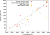 |
Fig. 3 Revised photospheric to spot temperature. Original photometric data points from Berdyugina (2005) are shown as light blue open circles. Doppler imaging values are shown as filled red circles where the values are taken from Table 1 and the values for the Sun are shown as two large open light blue circles with a temperature of 5800 K. The fit parameters are shown Equation (1) and summarised in Table 5. |
2.3.2 CRX-gradient and length
The simulations of Baroch et al. (2020) show that the gradient of the CRX-RV relation is an important diagnostic as it provides a key insight into how quickly the RV variations induced by a cool starspot decrease as a function of increasing (logarithmic) wavelength. In the simulations of Baroch et al. (2020), the CRX-gradient primarily depends on the spot-to-photosphere temperature contrast ratio for the case of one large spot located at a latitude of 78°. In addition to the CRX-gradient, Baroch et al. (2020) also reported that the length of the CRX-index versus RV relation depends on both the spot-to-photosphere contrast and the spot filling factor. This is expected because for a given single spot size (i.e. a star with a fixed filling factor), the wavelength-dependent RV amplitude and, hence, the gradient measured by the CRX-index is larger for a larger spot-to-photosphere contrast. Similarly, for a fixed spot-to-photospheric contrast, increasing a spot’s size (and thus the spot filling factor) will also lead to a greater CRX-length.
The models of Baroch et al. (2020) considered the impact of one starspot located at high latitudes on the surface of the mid-M dwarf YZ CMi. However, the results from Doppler imaging studies (examples are listed in Table 1) show that in reality, the surfaces of M dwarfs are likely to be much more densely spotted. In this work we use the CRX-gradient and the CRX-length as the two main diagnostic parameters of our investigation. We investigate how the CRX-gradient and CRX-length of stars in the CARMENES GTO sample depend on their fundamental stellar parameters and levels of stellar activity.
3 Data
3.1 Observations and data processing
The data investigated in this work comprise the full set of CARMENES Guaranteed Time Observations (GTO) of more than 350 M dwarfs which have been observed since the start of the CARMENES GTO survey in 2016. The CARMENES spectrograph is installed at the 3.5 m telescope at Calar Alto Observatory in Spain. It comprises two fibre-fed and cross-dispersed spectrographs, one at visible wavelengths (VIS, 520–960 nm) and the other at near-infrared wavelengths (NIR, 960–1710 nm) with a resolution of ~94 600 in the VIS and ~80 400 in NIR and an average sampling of 2.8 pixels (Quirrenbach et al. 2018). The data were processed in the usual manner for CARMENES data, namely, with caracal (CARMENES reduction and calibration software; Zechmeister et al. 2014; Caballero et al. 2016), and the RVs were calculated using serval (Spectrum radial velocity analyzer Zechmeister et al. 2018) using weighted averages to account for the wavelength dependence of the RVs, where the individual orders are weighted. The impact of telluric lines on the measured RVs was removed (Nagel et al. 2023) using the template division telluric modeling technique. The nightly zero points (NZPs) were also subtracted from the serval RV measurements (see Sect. 4.4 of Ribas et al. 2023 for a detailed explanation).
3.2 CARMENES NIR channel
In this work, we only use data from the CARMENES VIS channel and not from the CARMENES NIR channel because the NIR channel yields RV measurements that are less precise than the VIS channel. This is partly because of the diminished RV information content in the observed NIR domain Reiners et al. (2018). However, the CARMENES NIR channel also suffered from thermo-mechanical instability since the start of operations and until some corrective measures were applied a few years later. Consequently, the NIR RV data were in general not used during the exploitation of guaranteed time observations (however, see Morales et al. 2019 and Bauer et al. 2020). Subsequent instrument upgrades have dramatically improved the precision of the NIR channel (Schaefer et al., in prep.; Varas et al., in prep.) and a careful analysis of the newly collected NIR data is undergoing within the CARMENES consortium.
3.3 Activity indices and CCF parameters
Given the broad wavelength coverage of CARMENES, we have a large number of activity indicators available. We used a total of 26 indicators, as follows:
Six RV, CRX and differential line widths (dLW) calculated by serval – namely, RVVIS and RVNIR, CRXVIS and CRXNIR, and dLWVIS and dLWNIR.
Sixteen activity indices at VIS and NIR wavelengths computed following the procedure described by Schöfer et al. (2019). The full list of spectral line indices comprise: log(LHα/Lbol), pEW(Hα), HeD3, NaD, Ca IRT-a,-b,-c, He I 10830, Pa β, CaH2, CaH3, TiO 7050, TiO 8430, TiO 8860, VO 7436, VO 7942, and FeH Wing-Ford. We define stars with positive pEW(Hα) as having Hα in absorption, while Hα inactive stars have negative values and Hα active stars are where Hα is in emission. The minimum detectable emission in the Hα line depends on the resolution of the spectrograph and the signal-to-noise ratio (S/N) of the data and has been shown by Schöfer et al. (2019) to be −0.3 Å for CARMENES.
Four cross-correlation function (CCF) parameters, CCF-contrast, CCF-RV, CCF-FWHM, and CCF-BIS were computed following Lafarga et al. (2020).
3.4 CRX-all sample
From the full CAMRENES GTO sample, firstly, we selected stars with a minimum number of observations, Nobs > 25. This is the minimum number of observations required to give a reliable CRX-index versus RV relation and to provide a statistically significant correlation with activity indicators. The CARMENES GTO sample with Nobs > 25 comprises a total of 225 stars and is referred to as CARMENES NGTO25 sample in the rest of this work. Parameters for all 225 CARMENES NGTO25 stars are listed in Table B.1.
We then computed the statistical significance of the correlation of CRX-index with RV for each of the 215 stars using Pearson’s r coefficient. We defined a strong correlation (or anti-correlation) where Pearson’s r > |0.7|, and a moderate correlation to be 0.5 < |r| < 0.7. The statistical significance is computed by the Student’s t-test probability value, p. We assumed that values of p < 0.03 imply no strong evidence to reject the (no correlation) null hypothesis. There are a total of 39 stars with a strong or a moderate correlation and these stars are referred to as CRX-all in the work that follows and are listed in Table A.1. From these, there are 21 stars with a strong correlations between the CRX-index and RV and 18 stars have a moderate correlation.
3.5 CRX-slope sample
The CRX-all sample is further classified based on a visual inspection of the CRX-index versus RV relation for each star. A total of 13 stars exhibit a tight linear CRX-index versus RV relationship and comprise both strong and moderate statistical CRX-index versus RV correlations. This sample is referred to as the CRX-slope sample in the rest of this work. To avoid confusion, we refer to the actual measured value of the CRX slope as the CRX-gradient in the rest of this work. The CRX-index versus RV relation is shown for each of these stars in Fig. A.1.
3.6 CRX-Pearson sample
The 26 remaining stars are refereed to as the CRX-Pearson sample in the rest of this work. They were subdivided into Pearson-strong sample comprising 9 stars and Pearson-moderate sample comprising 17 stars. The CRX-index versus RV for these two samples are respectively shown in Fig. A.2 and Fig. A.3 The RV-CRX correlation deviates from a straight line in this sample, where the deviations can take the form of a high degree of scatter or a generally extended cloud shape. The reasons for these deviations are not well understood and are beyond the current scope of this work.
Sample Summary:
CRX-all: 39 stars with Pearson’s strong, |r| ≥ 0.7 (21 stars), or moderate, 0.5 < |r| < 0.7 (18 stars) correlations.
CRX-slope: 13 stars with a tight linear relationship, as inspected visually; they are a subset of the CRX-all sample.
CRX-Pearson: 26 stars with non-linear but moderate (17 stars) or strong (9 stars) Pearson’s r values.
3.7 Comparison to the CARMENES NGTO25-sample
The distribution of the CRX-all stars compared to the CARMENES NGTO25-sample in terms of spectral type and projected stellar rotational velocity, or v sin i is shown in Fig. 4. The 39 stars in the CRX-all sample cover all spectral types and broadly follows the spectral type distribution of the CARMENES NGTO25-sample. The distribution of v sin i values for the CRX-all stars and the CARMENES NGTO25-sample are shown in Fig. 4 (right panel). Approximately one-third of the CRX-all stars have v sin i values <2.0 km s−1, one-third have v sin i values between 2.0 and 4.0 km s−1 and the remaining third have values 4.0–10.5 km s−1. The wavelength dependence of the RVs depends on many fundamental stellar parameters. In the following sections, we investigate the correlations and trends in the activity indices available from the CARMENES spectra.
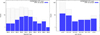 |
Fig. 4 Spectral type distribution (left panel) and the distribution of v sin i of the CRX-all sample, coloured in blue. Also shown are all of the CARMENES GTO stars with more than 25 observations as indicated by shaded grey bars. |
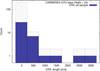 |
Fig. 5 Distribution of CRX-length for the CARMENES GTO sample (light grey) and the CRX-all sample (navy). For clarity, the CRX-length values of the CARMENES GTO sample are only shown up to a value of 3000 m s−1. |
4 Results: CRX gradient and length
As previously discussed, preliminary models indicate that the two most useful parameters to characterise the CRX-index versus RV relation are its gradient and length. For the CRX-slope sample, the measured CRX-gradient values typically have slopes ranging from −2.65 Np−1 to −3.70 Np−1 (eight stars), with four stars having slopes in the range −4.6 Np−1 to −17 Np−1, and one star having a very shallow slope of −1.16 Np−1. The colouring of points in Fig. 6 and subsequent figures is chosen to reflect these broad groupings. We caution the direct interpretation of the steepest slopes for the three stars with the latest M-dwarf spectral types as for these stars there is less flux in the bluer orders and may potentially bias the results. Since our aim is to apply uniform analysis to all stars we have included these stars but do not draw any conclusions from them. In contrast, the steep slope of the young M3.0 dwarf K2-33 results from very high levels of stellar activity given its young age.
The CRX-length values range from 30 m s−1 also for the M 2.5 dwarf TYC 3529-1437-1 to 2897 ms−1 for the M 3.0 dwarf K2-33. The distribution of CRX-length values for the CRX-all sample compared to the CARMENES GTO sample is shown in Fig. 5. In the work that follows, we normalise the CRX-length by dividing the measured length by the stellar v sin i.
Furthermore, in Fig. 6 we show the CRX variation, CRXmax − CRXmin, as a function of the total RV variation, RVmax − RVmin, which we define as the CRX-length. The CRX-slope stars with moderate gradients show a linear increase with increasing RV variation.
Figure 7 illustrates the correlation between the CRX-length and the Pearson’s r value, where longer CRX-length/v sin i values have a higher Pearson’s r value, indicating a stronger statistical correlation. We note that low CRX-length values occur at low v sin i values. There was no correlation noted between the CRX-gradient and the Pearson’s r value. We further investigated the correlation of CRX-gradient with the CRX-length. We find no correlation between these two parameters (plots not shown). We also examined the dependence of the CRX-gradient on the inferred spot-to-photospheric temperature contrast (see Sect. 2.3.1). While the results do not show a correlation with CRX-gradient, the CRX-slope stars lower contrasts for stars with higher CRX-length/v sin i values as shown in the middle panel of Fig. 7. Stars with low v sin i values show the lowest CRX-length/v sin i values over a range of medium to high contrasts. Increasing the v sin i value for a given contrast often results in a higher CRX-length/v sin i value. The lower panel of Fig. 7 shows that there is a tendency of stars with short stellar rotation periods to show slightly higher CRX-length/v sin i values.
Our initial results indicate that the interpretation and understanding the nature of the CRX is more challenging than suggested by the models (Baroch et al. 2020). However, it should be noted that only one starspot was modelled on the surface of YZ CMi and the reality is certainly more complicated. In general, M dwarfs are likely to have more complicated distributions of starspots, where the latitude of the starspot will also have an impact on the CRX-gradient and length (Barnes et al. 2011), as well as plage regions (Meunier et al. 2010; Jeffers et al. 2014). Given that M dwarfs typically have much lower levels of convective blueshift compared to the more massive G and K dwarfs, its impact on the RV precision is unlikely to be a large effect (Liebing et al. 2021) compared to more massive solar-type stars. The dependence of the CRX gradient and length as a function of stellar activity parameters is investigated in later sections of this work.
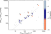 |
Fig. 6 Variation among CRX (CRXmax − CRXmin) as a function of RV variation (CRX-length = RVmax − RVmin). A straight line is fitted to moderate slopes (coloured navy). Points are coloured by CRX-gradient. The parameters of the fitted straight line are summarised in Table 5. |
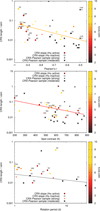 |
Fig. 7 Dependence of the CRX-length as a function of Pearson’s r value (upper panel), spot contrast (middle panel), and rotation period (lower panel) for the CRX-all stars sample. Closed symbols indicate Hα active stars and open symbols Hα inactive stars. Points are coloured by projected stellar rotational velocity (v sin i). The CRX-slope stars are labelled as indicated in Table A.1. In the top panel, the two arrows indicate two stars with positive Pearson’s r correlation. Their true Pearson’s value is shown in the label for each point. The parameters of the fitted straight lines are summarised in Table 5. |
4.1 Dependence on activity indicators
In this section, we investigate how the CRX gradient and CRX-length of each of the 13 CRX-slope stars depend on their measured activity indices in relation to the CRX-Pearson and CARMENES NGTO25-samples. The general patterns of activity in the CARMENES GTO sample have previously been presented and discussed in detail by Jeffers et al. (2018).
In Figs. 8–13, the stars in the CRX-slope sample are shown as diamond symbols, CRX-Pearson strong stars with an asterisk symbol, CRX-Pearson moderate stars as a cross, and the remaining stars in the CARMENES NGTO25-sample are shown as small grey circular points. In each figure, the left and right panels are colour-coded based on the CRX gradient and the CRX-length/v sin i, respectively.
The colouring for the CRX gradient and the CRX-length plots were chosen to represent the sample in terms of global groups rather specific stars. In the text that follows we discuss these plots in terms of the shallowest to the steepest slopes, and the shortest to the longest CRX-length values. The stellar activity indices that we investigate are stellar (i) rotational velocity or v sin i (Fig. 8) (ii) chromospheric emission via Hα (Fig. 9), (iii) diagnostic of spot coverage via TiO7050 Å band (Fig. 11), and finally (iv) average magnetic field strength (Fig. 13).
4.2 CRX-gradient
In Table 2, we have summarised the information contained in the left-hand panels of Figs. 8 – 13 to understand how the CRX gradient varies as a function of a range of stellar activity parameters. Comparing the gradients of the CRX-slope sample with the full CARMENES NGTO25-sample (see Jeffers et al. 2018), we conclude that the stars with the shallowest CRX-gradients are among the least active stars. Since there is only one star in this category, we did not include the shallowest slopes in Table 2. Stars with moderate CRX gradients occur at early to mid-M spectral types, with high levels of stellar activity (Figs. 8 and 9) and show saturated log(LHα/Lbol) and average magnetic field strengths (Figs. 10 and 13). Similarly, the steepest slopes occur at later M spectral types at moderate levels of activity (e.g. v sin i and log(LHα/Lbol); see Figs. 8 and 9). These stars show saturation at lower log(LHα/Lbol) values compared to stars with mid-M spectral types (Mohanty & Basri 2003). This is shown in Figs. 10 and 13.
4.3 CRX-length
The correlations between the CRX-length, v sin i, and the stellar activity indicators as shown in the right-hand panels of Figs. 8–13 are summarised in Table 3 for ease of comparison. Generally, the shortest CRX-lengths are found for stars with low to moderate Hα activity levels, with early to mid-M spectral types and moderate average magnetic field strengths (Figs. 8, 9, and 13). The moderate CRX-length values occur for very active stars and the longest lengths are for very active stars at late M spectral types. As noted in for the CRX gradient, activity in the latest M dwarfs saturates at lower log(LHα/Lbol) values compared to mid M dwarfs (Figs. 10 and 13).
CRX-gradient with activity.
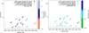 |
Fig. 8 Variation of projected rotational velocity (v sin i) as a function of spectral type for the CARMENES GTO sample with Nobs > 25. Stars in the CRX-slope sample are coloured according to the measured gradient(left panel) and CRX-length (right panel). Stars in the CRX-slope sample that are Hα active are indicated by closed symbols and Hα inactive stars as open symbols. The minimum v sin i value plotted is 2 km s−1. The stars are labelled as indicated in Table A.1. |
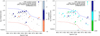 |
Fig. 9 Normalised Hα luminosities as a function of spectral type for CARMENES GTO sample with Nobs > 25. The solid orange line indicates the minimum values of emission in the Hα line that our CARMENES observations can detect, which is defined to be pEW (Hα) = −0.3 Å (Schöfer et al. 2019). A population of extremely active stars with pEW(Hα < −8.0 are indicated by the solid blue line as previously noted by Jeffers et al. (2018). Hα inactive stars are shown at the base of each plot as indicated by the y-axis. The stars in the CRX-slope sample are indicated by the diamond shapes which are coloured based on the CRX gradient of the data points in the left panel and CRX-length in the right panel. The stars are labelled as indicated in Table A.1. |
CRX-length with activity.
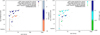 |
Fig. 10 Normalised Hα luminosities as a function of projected rotational velocities (v sin i) for CARMENES GTO sample with Nobs > 25. Stars in the CRX-slope sample are shown by diamond shaped point which are open for Hα inactive stars and filled for Hα active stars. The CRX-slope sample stars are coloured based on CRX-gradient (left panel) and CRX-length (right panel). The stars are labelled according to the same indications as in Table A.1. |
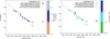 |
Fig. 11 Variation of TiO 7050 index as a function of stellar spectral type for the CARMENES GTO sample with Nobs > 25. The CRX-slope sample of stars is indicated by diamonds which are filled for Hα active stars and open for Hα inactive stars. The CRX-slope sample stars are coloured depending on CRX-gradient (left panel) and CRX-length (right panel). The stars are labelled as indicated in Table A.1. |
4.4 CRX-Pearson
The remaining stars in the CRX-Pearson sample follow the same trends. Stars with a strong Peason’s correlation typically have longer lengths and are located at mid to late M spectral types. The correlation of the CRX-length with various parameters was previously discussed in more detail in Sect. 3.
Stars not showing a CRX slope.
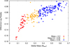 |
Fig. 12 Difference in Rossby number as a function of stellar mass derived using the fit in Eq. (2) and the parameters published in (Wright et al. 2018, their Eqs. (5) and (6)). Points are coloured by stellar mass following Shan et al. (2024). |
4.5 Noteworthy points
Our aim has been to present the results of the CRX-gradient and length in the context of stellar activity in a clear and concise manner. In addition to the points discussed above, there are a few noteworthy points to add, listed below.
Ca II H&K: We also investigated the dependence of the CRX on the Ca II H&K lines, derived for the CARMENES GTO sample by Perdelwitz et al. (2021). However, there were only a few measurements available for the stars in the CRX-all sample from archival observations and it was not possible to determine any distinct correlations or trends; therefore these plots are not shown.
-
X-ray: As summarised in Tables 2, and 3, the X-ray data were only available for a small number of stars and it was not possible to derive any trends or correlations. As part of determining the log(Lx/Lbol) relation as a function of Rossby number, we noticed that the fit parameters provided by Wright et al. (2018) in their Eqs. (5) and (6) contain typos, thus, are not the exact values derived from fitting the data in their Table 3. Notably, Reiners et al. (2022) independently found that there was an offset with the log τ values from Wright et al. (2018) for very low mass stars. The correct scaling for the empirical calibration data of Wright et al. (2018) is as follows (as an update to their Eqs. (5) and (6)):
![$\[\log \tau=(0.58 \pm 0.04)+(0.28 \pm 0.01)(V-K s),\]$](/articles/aa/full_html/2025/04/aa47510-23/aa47510-23-eq2.png) (2)
(2)
![$\[\qquad\quad\log \tau=(2.30 \pm 0.06)-(1.38 \pm 0.245)(M / M_{\odot})\\+(0.22 \pm 0.19)(M / M_{\odot})^{2},\]$](/articles/aa/full_html/2025/04/aa47510-23/aa47510-23-eq3.png) (3)
(3)where log τ is the convective turnover time and (V − Ks) is the magnitude difference between the V and Ks bands. The difference in the Rossby numbers derived using the fit parameters directly taken from Wright et al. (2018) and Eq. (2) is illustrated in Fig. 12 for the CARMENES GTO sample.
4.6 Stars not showing CRX-gradient
To understand why some stars show a clear CRX slope or have a statistically significant correlation between CRX and RV, and other stars not, we inspected the CRX-index versus RV relations of seven stars that are not part of the CRX-all sample. These stars were selected from regions that did not contain any stars from the CRX-all sample in (i) the v sin i versus spectral type and (ii) the Hα versus spectral type plots. The stars are listed in Table 4 and their CRX-index versus RV relations are shown in Appendix A.4. The two stars, Teegarden’s star and K2-18 are exoplanet hosts (Zechmeister et al. 2019; Sarkis et al. 2018; Plavchan et al. 2020; Martioli et al. 2021; Wittrock et al. 2022; Dreizler et al. 2024). For both Teegarden’s star and K2-18, the planet-induced RV amplitude is a large fraction of the CRX-length value. In particular, K2-18 has been reported by Radica et al. (2022) to exhibit a wavelength dependence in RV based on the line-by-line method, but this is below the Pearson’s r threshold of 0.5 we are considering in this work.
5 Results: Removing stellar activity from RVs using CRX
The RV signatures resulting from presence of stellar activity, such as spots and plage regions, is wavelength dependent, due to the decrease of the photospheric-and-spot contrast; whereas a planetary companion would induce a RV signal that is wavelength independent. In this section, we use the wavelength-dependent information parameterised by the CRX to remove the signatures of stellar activity from the CRX-all sample of 39 stars. The subtraction of the CRX, via a linear fit to the CRX-RV anti-correlation, from the RV results in a decrease in the RV rms by a factor of up to 3.89 in the case of 1RXS J050156.7+4233 (labelled: 1RX). The results for the CRX-all sample are listed in Table A.1. We found a total of nine stars, making up 25% of the CRX-all sample, with a factor of improvement greater than 2.0.
There is a strong dependence of the factor of improvement (FoI) with Pearson’s r value, as shown in the top left-hand panel of Fig. 14. A linear fit shows that this relation can be expressed as
![$\[\\begin{array}{ll}\mathrm{FoI}=-18.51 r-14.48 & (r<-0.80), \\ \mathrm{FoI}=-1.98 r+0.04 & (r>-0.80),\end{array}\]$](/articles/aa/full_html/2025/04/aa47510-23/aa47510-23-eq4.png) (4)
(4)
where FoI is the factor of improvement and r is the Pearson’s r value. Only three stars show an RV rms reduction that is greater than a factor of 3. These are 1RXS J050156.7+010845, YZ CMi and EV Lac, which will be referred to as the RVcorr3 stars in the rest of this work. All three stars have mid-M spectral types and are located on the saturated part of the rotation-activity correlation (Fig. 10). For mid-M spectral types, this occurs at higher normalised Hα values than for the latest M dwarf spectral types.
The correlation of the Factor of Improvement with stellar rotation period is shown in Fig. 14 (upper right panel). The highest factor of improvement values are shown for fast to moderately rotating stars with rotation periods of approximately a few days to just less than ten days. This is likely because such moderately rotating stars have more stable spot patterns.
The TiO indicator can be considered as an indicator of dark starspot coverage, even on slowly rotating and less active stars Vogt (1979); Amado & Zboril (2002); O’Neal et al. (2004). To remove the spectral type dependence that we previously showed in Fig. 11, we plot the maximum minus the minimum value for each star (Fig. 14, middle left panel). The RVcorr3 stars show moderate values, while the cluster of low v sin i stars with very small factor of improvement values show very small TiO 7050 variations.
Furthermore, we show the factor of improvement as a function of normalised Hα in Fig. 14 (middle row right panel). Notably, the RVcorr3 stars have very high levels of Hα activity. The remaining stars show Hα values spanning the full range from low to high levels of Hα activity.
Finally, in the lower panels of Fig. 14, we investigate the dependence of the factor of improvement value on the CRX-length/v sin i and spot contrast ratio (left and right panels respectively). The factor of improvement increases with increasing CRX-length/v sin i values, though importantly the RVcorr3 stars don’t follow this trend with the highest factor of improvement values and moderate CRX-length/v sin i values. The lowest v sin i stars have the lowest factor of improvement values and the lowest CRX-length/v sin i measurements. The variation of the factor of improvement with spot contrast ratio shows a general trend of increasing factor of improvement values with decreasing spot contrast ratios. The highest factor of improvement values occurring for moderate spot coverage ratios that are typical for mid-M spectral types.
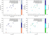 |
Fig. 13 Average magnetic field strength as a function of spectral type (upper panels) and v sin i (lower panels) for the CARMENES GTO sample with Nobs > 25. Stars in the CRX-slope sample are indicated by diamonds and are coloured according to CRX-gradient (left panel) and CRX-length (right panel). The minimum v sin i value plotted is 2 km s−1. The stars are labelled as indicated in Table A.1. |
6 Discussion
The advantage of the CARMENES spectrograph is its large wavelength coverage and high RV precision. In this work we have investigated the wavelength dependence of RVs for the CARMENES NGTO25 sample of 215 stars. In this section, we discuss our results.
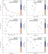 |
Fig. 14 Factor of improvement in the RV rms from the subtraction of the RV estimated from the RV-CRX correlation for each star in the CRX-all sample. Filled points indicate Hα active stars while open points show Hα inactive stars. Symbols are coloured based on CRX-gradient value or none (grey points). The factor of improvement is shown as a function of Pearson’s r (see Table 5 for parameters of the fit), stellar rotation period (upper row, left and right), stellar TiO7050 max-min value (using 95% percentiles) and normalised Hα luminosity (middle row left and right) and CRX-length/v sin i and (zoomed) spot contrast ratio (lower row, left and right). The stars are labelled as in Table A.1. |
6.1 CRX-gradient and CRX-length as a function of stellar parameters
Our results show that from the CARMENES NGTO25 sample of 215 stars that 39 stars show a strong or a moderate correlation between the CRX and the RV (CRX-all stars). Furthermore, a subset of 13 of these stars show a tight linear relationship (CRX-slope stars).
We demonstrate that the larger the variation is in CRX-length/v sin i the larger the variation is in CRX (i.e. ΔCRX). The highest variations in CRX-length and CRX tend to occur for the least massive stars with the steepest CRX-gradients where their activity levels are saturated. The caveat with this is that these stars have very little flux at bluer wavelengths and may be biased. However, the very active star K2-22 also shows a very steep slope, but has a spectral type of M 3.0 V. This shows that our methods can detect a CRX-RV correlation even for more rapidly rotating stars with high levels of stellar activity.
There is also a strong dependence of the CRX-length/v sin i on the Pearson’s r value with the slowest rotating stars having the lowest CRX-length/v sin i values and, at most, moderate Pearson’s r values for the CRX-RV relation. This is in agreement with the previous work of Tal-Or et al. (2018). There is also a correlation of the CRX-length/v sin i with spot-to-photosphere temperature contrasts, where stars with lower contrasts (e.g. late-M spectral types) show higher CRX-length/v sin i values. While these results are valid for our sample of stars, a true determination of the inter-dependency between CRX-length/v sin i and the stellar spot-to-photosphere temperature contrast is only possible when we know the distribution and evolution of spots and other features of stellar activity on the stellar surface. As noted by Barnes et al. (2011), the latitude of a starspot (or other activity signature) will impact the activity induced RV, with higher latitude spots having a lower RV than equatorial spots. Similarly, the latitude of spots will impact the lemniscate shape (Boisse et al. 2011). We already know from our extensive investigation of stellar activity the CARMENES consortium that every M dwarf is singular when it comes to its activity patterns and evolution timescales.
6.1.1 Dependence of CRX-gradient on stellar activity
Since there is only one star classified as having a shallow CRX-gradient, we restricted the discussion of our results to the stars with moderate and steep slopes. The stars in the CRX-slope sample with moderate CRX-gradients cover a range of spectral types from early-M to mid-M, as indicated by the navy points in Figs. 8–13. These stars are active stars, as evidenced by: (i) higher v sin i values of up to 5 km s−1 for stars with early-M spectral types and a range of v sin i values from 2 to 11 km s−1 at mid-M spectral types (Fig. 8); (ii) a range in rotation periods from 1 to 11 days; (iii) the highest log(LHα/Lbol) values (Fig. 9) in the CRX-all sample of 39 stars; (iv) located in the upper part of the log(LHα/Lbol) as a function of v sin i (Fig. 10); (v) lowest TiO7050 values per spectral type bin (Fig. 11); (vi) saturation in X-rays (not shown); and (vi) highest average magnetic field strengths as a function of spectral type and v sin i (Fig. 13, upper and lower panels respectively). Also, for our M-dwarf sample, they exhibit comparatively high to moderate ΔT spot-and-photosphere temperature contrasts.
There are only a few stars with high CRX-gradient values and the latest spectral types among the CRX-slope sample. Despite their high-CRX-gradients, these stars exhibit moderate levels of activity (i) they have moderate to high v sin i levels (Fig. 8); (ii) are the most Hα active stars in the CARMENES NGTO25-sample for the latest spectral types (Fig. 9); (iii) are located in the active part of the log(LHα/Lbol) as a function of v sin i (Fig. 10); (iv) are located in the ‘hook’ part of the TiO7050 per spectral type bin (Fig. 11); and (v) show moderate average magnetic field strengths as a function of spectral type and v sin i (Fig. 13, upper and lower panels respectively). Their moderate activity is because late-M dwarfs saturate at lower activity levels compared to early and mid-M dwarfs (for more details see Mohanty & Basri 2003). These stars have the smallest ΔT spot and photosphere temperature contrasts. As previously explained, we advise caution in the literal interpretation of these steep slopes, as they may be biased due to the lack of flux at blue orders, compared to the rest of the sample.
6.1.2 Dependence of CRX-length on stellar activity
The stars with the shortest CRX-length values have mid-M spectral types and show low to moderate levels of stellar activity as evidenced by (i) their low v sin i values (Fig. 8) and a range of moderate rotation periods (Fig. 7); (ii) are the least Hα active stars (Fig. 9); (iii) are located in the unsaturated part of the rotation-activity relation (Fig. 10); and (iv) have low to moderate average magnetic field strengths and are located on the unsaturated part of the magnetic field-rotation relation (Fig. 13, lower and upper panels, respectively).
Stars with moderate CRX-length values typically are early to mid-M dwarfs with moderate to high levels of stellar activity. This is shown by (i) their increased v sin i levels and short rotation periods (Fig. 8); (ii) generally the Hα activity levels for their spectral types (Fig. 9); (iii) that they are mostly located on the saturated part of the rotation-activity relation (Fig. 10) and X-ray distributions (not shown); and (iv) highest average magnetic field strengths for their spectral types (Fig. 13 upper and lower panels).
As we know that the late-M dwarfs become saturated in terms of activity, we already know what to expect. The CRX-length is longest for the stars with mid- to late-M spectral types. Compared to the CARMENES NGTO25 sample, they are not the most active stars, in both Hα and average magnetic field strengths, for their spectral types; however, they do have moderate to fast v sin i values and short rotation periods (Fig. 8). Their normalised Hα levels are close to or above the blue line (indicating very high levels of Hα activity) in Fig. 9 and are on the saturated part of the rotation-activity relation in Figs. 10 and 13. They also cover the ‘hook’ in the TiO distribution with spectral type.
6.2 Average magnetic field strength
The average magnetic field strengths were computed from the telluric corrected co-added templates with exceptionally high S/N values (Reiners et al. 2022). The CRX-gradient shows moderate values for the stars with the highest average magnetic field strengths at mid-M spectral types. The average magnetic field strength have been shown by Haywood et al. (2014, 2022) to be a proxy of RV variations in the Sun and other stars in agreement with Meunier et al. (2010). Recently, the work of Ruh et al. (2024) investigated the RV jitter and its relation to the average magnetic field strength. They showed that M dwarfs with excess activity-rotation induced RV jitter have magnetic field filling factors that are dominated by a component with a strength of 2–4 kG.
6.3 Correlations with bisector inverse span (BIS)
All of the CRX-all stars have a strong or moderate (anti-) correlations between CRX and moment 1 indicators such as RV. Recent models of stellar activity and its impact on the line moments, Barnes et al. (2024) showed that there is a high likelihood of having correlations between odd numbered moments, such as moment 1 (e.g. RV) and moment 3 (e.g. the BIS). While the CRX-index and BIS measure different aspects of the stellar spectra, it is important to also note that the BIS also includes a chromatic effect. This is because the skewness of the line profile is caused by the different velocity patterns as a function of formation depth, with redder lines being weaker.
Given the similarity of the lemniscate shape of the CRX and the BIS (see for e.g. Boisse et al. 2011), we additionally investigate the statistical correlation between the CRX and BIS (moment 3 line moment). We use Pearson’s r for the 39 stars in the CRX-all sample. Our results are shown in Table A.1 and confirm that moment 1 and moment 3 are linked with 13 stars having either a strong or a moderate Pearson’s r value between the CRX and BIS. The 3 stars that show the highest factor of improvement also show a strong correlation between CRX and BIS (see Table A.1). This is in agreement with our previous observational results for the mid-M dwarf EV Lac (Jeffers et al. 2022), the results of Schöfer et al. (2022) for four stars in the CARMENES sample.
Recently, Lafarga et al. (2021) investigated the optimal activity indicators to identify activity induced RV signals in M dwarf stars with a range of activity levels. They reported that the CRX and BIS are the most effective indicators for tracing activity in high-mass and high-activity (measured by Hα) M dwarfs. A total of nine CRX-slope and four CRX-Pearson stars are also included in their sample, where for each of these star the stellar rotation period is detected in the RV (nine CRX-slope, four CRX-Pearson) and the CRX (nine CRX-slope, one CRX-Pearson). A total of six CRX-slope stars and three CRX-Pearson stars have both a periodic signal detected at the stellar rotation period in BIS.
Previously, the results of Saar & Donahue (1997) reported that the BIS span varies as (v sin i)3.3. In Fig. 15, we show the distribution of v sin i of the CRX-all sample where the distribution of the stars with a strong or a moderate correlation between the CRX-index and the BIS are highlighted. Our results show that BIS is a significant parameter, at moderate v sin i rates and even at low v sin i levels. While models of fixed starspots are important, a comprehensive analysis also needs to take into account the variations in the latitude, longitude, and lifetimes of the spot distributions over the time span of data collection.
Relations derived in this work.
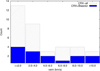 |
Fig. 15 v sin i distribution of all 39 stars in the CRX-all sample (CRX-slope and CRX-Pearson) shown as grey shaded bars. The stars with a strong or a moderate correlation of the CRX with BIS are shown in blue. |
6.4 Subtraction of the CRX
The subtraction of a linear fit of the CRX-RV anti-correlation from the RV results in a reduction of the RV rms by a factor of up to 4. There is a tight correlation of factor of improvement with Pearson’s r for both the CRX-slope and Pearson-all samples, where the best stars typically have rotation periods of several days (Fig. 14 top panels), low levels of Δ TiO and very high Hα values (Fig. 14 middle panels), and moderate CRX-length/v sin i values and low to moderate M dwarf spot contrasts. The moderate rotation periods and low Δ TiO values point to stable spot feature, although the high Hα values could result from plage regions appearing dark at the limb centre, as suggested in the work by Johnson et al. (2021).
Whether the star has a moderate or a steep CRX-gradient does not influence the factor of improvement values. However, in both the Δ TiO and the Hα activity relations, the CRX-slope stars with the steepest gradients occupy a separate branch or region compared to the CRX-slope stars with moderate gradients. Furthermore, we show that all of the CRX-slope stars with moderate gradients have CRX-length/v sin i values that are low to moderate (with the best factor of improvement values) and that the steepest gradients have the longest lengths. The stars with the longest CRX-length values are in the saturated regime of the rotation-activity plot and have moderate CRX slopes. These relations are summarised in Fig. 14 and Table 5.
6.4.1 Planet detection thresholds
We have demonstrated that the improvement in the RV rms by removing the contribution of the CRX can be up to a factor of nearly 4. The implications that this has for improving the detectability of small exoplanets was simulated using the dataset of EV Lac. An exoplanetary signal is first injected in the uncorrected data and then the activity contribution is removed (Cardona Guillén et al. 2023). With the linear correction factor it is possible to detect exoplanets that are approximately 2.5 times less massive, compared to the same dataset but without the correction. The exoplanetary signal can be identified even if it is not a significant signal in the original dataset. We will explore this further in forthcoming papers.
Other techniques that exploit the wavelength dependence of activity induced RVs include the work of Collier Cameron et al. (2021). They presented test simulations by adding injected signals of low-mass planets to five years of HARPS Sun-as-a-Star observations of the solar spectrum, where planets can be recovered with a precision of ~6.6 cm s−1.
In addition to using the wavelength dependence of RVs, there are currently a large number of methods in the literature to remove the impact of stellar activity. An excellent summary of these methods is presented by Meunier (2021) (see their Table 1). Also Zhao et al. (2022) presented the results of a comparison of different methods (expanding from the work of Dumusque et al. 2017) and concluded that no method is yet performing better than classical linear decorrelation, further supporting the results we obtained in this work.
6.4.2 Surface mapping
The large-scale magnetic field geometry has been reconstructed for a total of six stars in the CRX-all sample. From these six stars, YZ CMi and EV Lac are also part of the RVcorr3 stars with the highest reduction in RV rms after the subtraction of the CRX. V388 Cas, AD Leo, and OT Ser are CRX-slope stars, while AU Mic is a CRX-Pearson (moderate) star. The mid-M dwarfs YZ CMi and EV Lac consistently show an axisymmetric, predominantly poloidal, and simple large-scale magnetic field geometry that does not change significantly over time periods of approximately one year (Donati et al. 2008; Morin et al. 2008b, 2010). The long-term stability of YZ CMi enabled Baroch et al. (2020) to fit CARMENES data with one stable starspot. Recently, Jeffers et al. (2022) also reconstructed several low-resolution surface brightness maps of EV Lac using CARMENES data. These authors also found a long-term stable component with small-scale variability which is consistent with EV Lac’s TESS light curve.
The remaining three stars in the CRX-all sample with large-scale magnetic field maps show a variety of geometries. The mid-M dwarf V388 Cas exhibits a comparably simple large-scale magnetic field geometry as reconstructed for YZ CMi and EV Lac, which is also axisymmetric and predominantly poloidal. The large-scale magnetic field geometry of the mid-M dwarf AD Leo shows strong and simple magnetic features, which are mostly poloidal and axisymmetric and with low level variations over the time span of 1 year. On the other hand, the early-M dwarf OT Ser shows latitudinal rings of mixed polarities that are axisymmetric and dominated by the poloidal component, but also featuring a significant toroidal component (Donati et al. 2008; Morin et al. 2008b, 2010).
The active planet-hosting star AU Mic, which is a CRX-Pearson moderate star in this work, has been the focus of an intensive observational campaign to reconstruct its surface activity patterns (Klein et al. 2021, 2022). AU Mic has surface brightness features that evolve rapidly, which is consistent with its young age of 22 Myr and frequent flaring events (Robinson et al. 2001). We cannot exclude the possibility that the reason why AU Mic is not a CRX-slope star is that its stellar activity features evolved on a much shorter timescale, compared to the observational cadence of the CARMENES data of AU Mic. This may explain the curved nature of AU Mic’s CRX-RV relation (see Fig. A.3 and Cale et al. 2021).
These Zeeman–Doppler imaging (ZDI) observations point to that (1) early-M dwarfs have weak but complex fields and consequently activity patterns; (2) mid-M dwarfs have less complex but strong magnetic fields; and (3) late-M dwarfs can have either of these configurations. The results from brightness (Doppler) imaging typically exhibit more complex spot patterns for all M spectral types (Barnes & Collier Cameron 2001; Barnes et al. 2004, 2015, for example), but these results are biased towards stars with v sin i values that are in excess of 15–20 km s−1.
6.5 Data sampling
One point to consider is that the observations of the CARMENES GTO stars have been secured with the main aim of detecting close-in orbiting exoplanets; thus, the stellar activity of the target stars has not specifically been characterised. This means that there can be gaps in the observational time series longer than a few stellar rotation periods, which is the timescale on which we would expect stellar activity features, such as spots and plage regions, to evolve.
If the stellar activity features (and, consequently, the CRX) have evolved over this time frame, then determining the relevant correlations and removing the contribution of the CRX will be biased by the time sampling of the dataset. For example, the very detailed analysis of EV Lac by Jeffers et al. (2022) showed that it is possible to see additional (anti-)correlations between the line moments or parameters with smaller data sets that cover only a few stellar rotation periods and where the features of stellar activity have not significantly evolved. In this work, we have shown that the subtraction of the CRX from the RVs works optimally for moderate rotation periods, which is likely to result from a combination of stable global starspot patterns that are more likely to be well sampled by our CARMENES data.
For very active stars, with higher rotation periods, this could mean that the stellar activity features have evolved significantly over the timespan of the observations, whereas the more stable activity patterns are less impacted by the cadence of the observations. In the future, we will investigate whether the more rapidly evolving stellar activity can be mitigated using densely sampled observations covering a large wavelength range, such as those used by the RedDots exoplanet search programme (Jeffers et al. 2020).
7 Conclusions
In this work, we investigate the wavelength dependence of high-precision RV measurements via the CRX. We have drawn the following conclusions:
Approximately 17% of stars in the Carmenes GTO sample are CRX-all stars (i.e. stars with strong-moderate RV Pearson’s r correlations of CRX-index vs RV);
Dependence on stellar activity diagnostics shows that CRX-all stars have low to moderate activity levels and cover the full range of M dwarf spectral types from M1.5 to M8.5;
The variation of RVs with wavelength can be used to remove the impact of stellar activity with an improvement in the RV rms of up to a factor of 4. The optimal targets are moderately active stars with a tight CRX-RV correlation;
The correction effectiveness is related to the stability and structure of the activity patterns, although more active stars could be included with regular cadence or high-density sampled high-precision RVs;
The CRX provides an instantaneous decorrelation of activity-induced RVs.
The power of using the CRX as a diagnostic for activity-induced RV variation is that it is derived directly from the stellar spectra themselves. In the future we will expand this work to investigate the variation of the CRX for more magnetically active stars with simultaneous high-cadence observations spanning across multiple instruments.
Data availability
The figures in Appendix A are only available online at https://zenodo.org/records/14013877.
Table B.1 is available at the CDS via anonymous ftp to cdsarc.cds.unistra.fr (130.79.128.5) or via https://cdsarc.cds.unistra.fr/viz-bin/cat/J/A+A/696/A27
Acknowledgements
We would like to thank the referee for their very insightful and constructive comments which helped to improve the clarity of the paper. This publication is based on observations collected under the CARMENES Legacy+ project. CARMENES is an instrument at the Centro Astronómico Hispano en Andalucía (CAHA) at Calar Alto (Almería, Spain), operated jointly by the Junta de Andalucía and the Instituto de Astrofísica de Andalucía (CSIC). CARMENES was funded by the Max-Planck-Gesellschaft (MPG), the Consejo Superior de Investigaciones Científicas (CSIC), the Ministerio de Economía y Competitividad (MINECO) and the European Regional Development Fund (ERDF) through projects FICTS-2011-02, ICTS-2017-07-CAHA-4, and CAHA16-CE-3978, and the members of the CARMENES Consortium (Max-Planck-Institut für Astronomie, Instituto de Astrofísica de Andalucía, Landessternwarte Königstuhl, Institut de Ciències de l’Espai, Institut für Astrophysik Göttingen, Universidad Complutense de Madrid, Thüringer Landessternwarte Tautenburg, Instituto de Astrofísica de Canarias, Hamburger Sternwarte, Centro de Astrobiología and Centro Astronómico Hispano-Alemán), with additional contributions by the MINECO, the Deutsche Forschungsgemeinschaft (DFG) through the Major Research Instrumentation Programme and Research Unit FOR2544 “Blue Planets around Red Stars”, the Klaus Tschira Stiftung, the states of Baden-Württemberg and Niedersachsen, and by the Junta de Andalucía. This work was based on data from the CARMENES data archive at CAB (CSIC-INTA). We acknowledge financial support from the Agencia Estatal de Investigación (AEI/10.13039/501100011033) of the Ministerio de Ciencia e Innovación and the ERDF “A way of making Europe” through projects PID2021-125627OB-C31, PID2019-109522GB-C5[1:4] and the Centre of Excellence “Severo Ochoa” and “María de Maeztu” awards to the Instituto de Astrofísica de Canarias (CEX2019-000920-S), Instituto de Astrofísica de Andalucía (CEX2021-001131-S), and Centro de Astrobiología (MDM-2017-0737). This work was also funded by the Generalitat de Catalunya/CERCA programme, and the DFG through the priority programme SPP 1992 ‘Exploring the Diversity of Extrasolar Planets’ (Jeffers, JE 701/5-1).
Appendix A Supplementary information
Derived CRX parameters of the CRX-all stars sample.
References
- Amado, P. J., & Zboril, M. 2002, A&A, 381, 517 [NASA ADS] [CrossRef] [EDP Sciences] [Google Scholar]
- Barnes, J. R., & Collier Cameron, A. 2001, MNRAS, 326, 950 [NASA ADS] [CrossRef] [Google Scholar]
- Barnes, J. R., James, D. J., & Collier Cameron, A. 2004, MNRAS, 352, 589 [NASA ADS] [CrossRef] [Google Scholar]
- Barnes, J. R., Jeffers, S. V., & Jones, H. R. A. 2011, MNRAS, 412, 1599 [Google Scholar]
- Barnes, J. R., Jeffers, S. V., Jones, H. R. A., et al. 2015, ApJ, 812, 42 [Google Scholar]
- Barnes, J. R., Jeffers, S. V., Haswell, C. A., et al. 2017, MNRAS, 471, 811 [Google Scholar]
- Barnes, J. R., Jeffers, S. V., Haswell, C. A., et al. 2024, MNRAS, 534, 1257 [NASA ADS] [CrossRef] [Google Scholar]
- Baroch, D., Morales, J. C., Ribas, I., et al. 2020, A&A, 641, A69 [EDP Sciences] [Google Scholar]
- Bauer, F. F., Zechmeister, M., Kaminski, A., et al. 2020, A&A, 640, A50 [NASA ADS] [CrossRef] [EDP Sciences] [Google Scholar]
- Bean, J. 2020, American Astronomical Society Meeting Abstracts, 235, 225.04 [Google Scholar]
- Bellotti, S., Petit, P., Morin, J., et al. 2022, A&A, 657, A107 [NASA ADS] [CrossRef] [EDP Sciences] [Google Scholar]
- Berdyugina, S. V. 2005, Liv. Rev. Sol. Phys., 2, 8 [Google Scholar]
- Boisse, I., Bouchy, F., Hébrard, G., et al. 2011, A&A, 528, A4 [NASA ADS] [CrossRef] [EDP Sciences] [Google Scholar]
- Caballero, J. A., Cortés-Contreras, M., Alonso-Floriano, F. J., et al. 2016, Cambridge Workshop on Cool Stars, Stellar Systems, and the Sun, 148 [Google Scholar]
- Cale, B. L., Reefe, M., Plavchan, P., et al. 2021, AJ, 162, 295 [NASA ADS] [CrossRef] [Google Scholar]
- Cardona Guillén, C., Béjar, V. J. S., Lodieu, N., et al. 2023, A&A, submitted [NASA ADS] [CrossRef] [EDP Sciences] [Google Scholar]
- Carmona, A., Delfosse, X., Bellotti, S., et al. 2023, A&A, 674, A110 [NASA ADS] [CrossRef] [EDP Sciences] [Google Scholar]
- Collier Cameron, A., Ford, E. B., Shahaf, S., et al. 2021, MNRAS, 505, 1699 [NASA ADS] [CrossRef] [Google Scholar]
- Crass, J., Gaudi, B. S., Leifer, S., et al. 2021, arXiv e-prints [arXiv:2107.14291] [Google Scholar]
- Desort, M., Lagrange, A. M., Galland, F., Udry, S., & Mayor, M. 2007, A&A, 473, 983 [CrossRef] [EDP Sciences] [Google Scholar]
- Donati, J. F., Morin, J., Petit, P., et al. 2008, MNRAS, 390, 545 [Google Scholar]
- Dravins, D., Lindegren, L., & Nordlund, A. 1981, A&A, 96, 345 [NASA ADS] [Google Scholar]
- Dreizler, S., Luque, R., Ribas, I., et al. 2024, A&A, 684, A117 [NASA ADS] [CrossRef] [EDP Sciences] [Google Scholar]
- Dumusque, X., Boisse, I., & Santos, N. C. 2014, ApJ, 796, 132 [NASA ADS] [CrossRef] [Google Scholar]
- Dumusque, X., Borsa, F., Damasso, M., et al. 2017, A&A, 598, A133 [NASA ADS] [CrossRef] [EDP Sciences] [Google Scholar]
- Haywood, R. D., Collier Cameron, A., Queloz, D., et al. 2014, MNRAS, 443, 2517 [Google Scholar]
- Haywood, R. D., Milbourne, T. W., Saar, S. H., et al. 2022, ApJ, 935, 6 [NASA ADS] [CrossRef] [Google Scholar]
- Jeffers, S. V. 2005, MNRAS, 359, 729 [NASA ADS] [CrossRef] [Google Scholar]
- Jeffers, S. V., & Donati, J. F. 2008, MNRAS, 390, 635 [CrossRef] [Google Scholar]
- Jeffers, S. V., Barnes, J. R., Jones, H. R. A., et al. 2014, MNRAS, 438, 2717 [NASA ADS] [CrossRef] [Google Scholar]
- Jeffers, S. V., Schöfer, P., Lamert, A., et al. 2018, A&A, 614, A76 [NASA ADS] [CrossRef] [EDP Sciences] [Google Scholar]
- Jeffers, S. V., Dreizler, S., Barnes, J. R., et al. 2020, Science, 368, 1477 [Google Scholar]
- Jeffers, S. V., Barnes, J. R., Schöfer, P., et al. 2022, A&A, 663, A27 [NASA ADS] [CrossRef] [EDP Sciences] [Google Scholar]
- Johnson, L. J., Norris, C. M., Unruh, Y. C., et al. 2021, MNRAS, 504, 4751 [NASA ADS] [CrossRef] [Google Scholar]
- Jurgenson, C., Fischer, D., McCracken, T., et al. 2016, SPIE Conf. Ser., 9908, 99086T [Google Scholar]
- Klein, B., Donati, J.-F., Moutou, C., et al. 2021, MNRAS, 502, 188 [Google Scholar]
- Klein, B., Zicher, N., Kavanagh, R. D., et al. 2022, MNRAS, 512, 5067 [NASA ADS] [CrossRef] [Google Scholar]
- Kossakowski, D., Kürster, M., Henning, T., et al. 2022, A&A, 666, A143 [NASA ADS] [CrossRef] [EDP Sciences] [Google Scholar]
- Lafarga, M., Ribas, I., Lovis, C., et al. 2020, A&A, 636, A36 [NASA ADS] [CrossRef] [EDP Sciences] [Google Scholar]
- Lafarga, M., Ribas, I., Reiners, A., et al. 2021, A&A, 652, A28 [NASA ADS] [CrossRef] [EDP Sciences] [Google Scholar]
- Lagrange, A. M., Desort, M., & Meunier, N. 2010, A&A, 512, A38 [NASA ADS] [CrossRef] [EDP Sciences] [Google Scholar]
- Liebing, F., Jeffers, S. V., Reiners, A., & Zechmeister, M. 2021, A&A, 654, A168 [NASA ADS] [CrossRef] [EDP Sciences] [Google Scholar]
- Lisogorskyi, M., Jones, H. R. A., & Feng, F. 2019, MNRAS, 485, 4804 [NASA ADS] [CrossRef] [Google Scholar]
- Martioli, E., Hébrard, G., Correia, A. C. M., Laskar, J., & Lecavelier des Etangs, A. 2021, A&A, 649, A177 [NASA ADS] [CrossRef] [EDP Sciences] [Google Scholar]
- Meunier, N. 2021, arXiv e-prints [arXiv:2104.06072] [Google Scholar]
- Meunier, N., Desort, M., & Lagrange, A. M. 2010, A&A, 512, A39 [NASA ADS] [CrossRef] [EDP Sciences] [Google Scholar]
- Mohanty, S., & Basri, G. 2003, ApJ, 583, 451 [NASA ADS] [CrossRef] [Google Scholar]
- Morales, J. C., Mustill, A. J., Ribas, I., et al. 2019, Science, 365, 1441 [Google Scholar]
- Morin, J., Donati, J. F., Forveille, T., et al. 2008a, MNRAS, 384, 77 [CrossRef] [Google Scholar]
- Morin, J., Donati, J. F., Petit, P., et al. 2008b, MNRAS, 390, 567 [Google Scholar]
- Morin, J., Donati, J. F., Petit, P., et al. 2010, MNRAS, 407, 2269 [Google Scholar]
- Nagel, E., Czesla, S., Kaminski, A., et al. 2023, A&A, 680, A73 [NASA ADS] [CrossRef] [EDP Sciences] [Google Scholar]
- O’Neal, D., Neff, J. E., Saar, S. H., & Cuntz, M. 2004, AJ, 128, 1802 [Google Scholar]
- Panja, M., Cameron, R., & Solanki, S. K. 2020, ApJ, 893, 113 [CrossRef] [Google Scholar]
- Pepe, F., Cristiani, S., Rebolo, R., et al. 2021, A&A, 645, A96 [NASA ADS] [CrossRef] [EDP Sciences] [Google Scholar]
- Perdelwitz, V., Mittag, M., Tal-Or, L., et al. 2021, A&A, 652, A116 [NASA ADS] [CrossRef] [EDP Sciences] [Google Scholar]
- Plavchan, P., Barclay, T., Gagné, J., et al. 2020, Nature, 582, 497 [Google Scholar]
- Queloz, D., Henry, G. W., Sivan, J. P., et al. 2001, A&A, 379, 279 [NASA ADS] [CrossRef] [EDP Sciences] [Google Scholar]
- Quirrenbach, A., Amado, P. J., Ribas, I., et al. 2018, Proc. SPIE, 10702, 107020W [Google Scholar]
- Quirrenbach, A., CARMENES Consortium, Amado, P. J., et al. 2020, SPIE Conf. Ser., 11447, 114473C [Google Scholar]
- Radica, M., Artigau, É., Lafreniére, D., et al. 2022, MNRAS, 517, 5050 [NASA ADS] [CrossRef] [Google Scholar]
- Reiners, A., Bean, J. L., Huber, K. F., et al. 2010, ApJ, 710, 432 [Google Scholar]
- Reiners, A., Zechmeister, M., Caballero, J. A., et al. 2018, A&A, 612, A49 [NASA ADS] [CrossRef] [EDP Sciences] [Google Scholar]
- Reiners, A., Shulyak, D., Käpylä, P. J., et al. 2022, A&A, 662, A41 [NASA ADS] [CrossRef] [EDP Sciences] [Google Scholar]
- Ribas, I., Reiners, A., Zechmeister, M., et al. 2023, A&A, 670, A139 [NASA ADS] [CrossRef] [EDP Sciences] [Google Scholar]
- Robinson, R. D., Linsky, J. L., Woodgate, B. E., & Timothy, J. G. 2001, ApJ, 554, 368 [Google Scholar]
- Ruh, H. L., Zechmeister, M., Reiners, A., et al. 2024, A&A, 692, A138 [NASA ADS] [CrossRef] [EDP Sciences] [Google Scholar]
- Saar, S. H., & Donahue, R. A. 1997, ApJ, 485, 319 [Google Scholar]
- Sarkis, P., Henning, T., Kürster, M., et al. 2018, AJ, 155, 257 [NASA ADS] [CrossRef] [Google Scholar]
- Schöfer, P., Jeffers, S. V., Reiners, A., et al. 2019, A&A, 623, A44 [Google Scholar]
- Schöfer, P., Jeffers, S. V., Reiners, A., et al. 2022, A&A, 663, A68 [NASA ADS] [CrossRef] [EDP Sciences] [Google Scholar]
- Shan, Y., Revilla, D., Skrzypinski, S. L., et al. 2024, A&A, 684, A9 [NASA ADS] [CrossRef] [EDP Sciences] [Google Scholar]
- Suárez Mascareño, A., Faria, J. P., Figueira, P., et al. 2020, A&A, 639, A77 [Google Scholar]
- Tal-Or, L., Zechmeister, M., Reiners, A., et al. 2018, A&A, 614, A122 [NASA ADS] [CrossRef] [EDP Sciences] [Google Scholar]
- Vogt, S. S. 1979, PASP, 91, 616 [Google Scholar]
- Waite, I. A., Marsden, S. C., Carter, B. D., et al. 2015, MNRAS, 449, 8 [CrossRef] [Google Scholar]
- Waite, I. A., Marsden, S. C., Carter, B. D., et al. 2017, MNRAS, 465, 2076 [Google Scholar]
- Wittrock, J. M., Dreizler, S., Reefe, M. A., et al. 2022, AJ, 164, 27 [NASA ADS] [CrossRef] [Google Scholar]
- Wright, N. J., Newton, E. R., Williams, P. K. G., Drake, J. J., & Yadav, R. K. 2018, MNRAS, 479, 2351 [Google Scholar]
- Zechmeister, M., Anglada-Escudé, G., & Reiners, A. 2014, A&A, 561, A59 [NASA ADS] [CrossRef] [EDP Sciences] [Google Scholar]
- Zechmeister, M., Reiners, A., Amado, P. J., et al. 2018, A&A, 609, A12 [NASA ADS] [CrossRef] [EDP Sciences] [Google Scholar]
- Zechmeister, M., Dreizler, S., Ribas, I., et al. 2019, A&A, 627, A49 [NASA ADS] [EDP Sciences] [Google Scholar]
- Zhao, L. L., Fischer, D. A., Ford, E. B., et al. 2022, AJ, 163, 171 [NASA ADS] [CrossRef] [Google Scholar]
All Tables
Empirical data used to derive spot-to-photospheric temperature contrasts using the Doppler imaging technique.
All Figures
|
Fig. 1 Illustration of the RV variation with wavelength, where the central wavelength is given for each order. Shown are the same data as in Fig. 2, with the steepest positive slope shown by red points. The green line indicates the slope of these points, which is the CRX-index for each individual spectrum. The weighted RV measurement is shown by the purple line. The wavelength spacing is logarithmic. |
| In the text | |
|
Fig. 2 Illustration of the behaviour of the CARMENES visible channel CRX for the mid-M dwarf EV Lac. Top-left: variation of RV as a function of wavelength (spacing is logarithmic). The CRX-index is the slope of RV vs log(λ) for each spectrum. A total of 10 CARMENES spectra are shown covering approximately one stellar rotation. The upper and lower boundaries are the fits to the most positive and negative RV values. Top right: The CRX-gradient, illustrating the CRX-index as a function of the ‘mean’ RV. Bottom-left and bottom-right: CRX vs. rotation phase and RV vs rotation phase illustrating the anti-correlation of CRX-index (i.e. the negative CRX-gradient shown in the top right panel). The plotted points in each panel are colour coded according to stellar rotation phase. |
| In the text | |
|
Fig. 3 Revised photospheric to spot temperature. Original photometric data points from Berdyugina (2005) are shown as light blue open circles. Doppler imaging values are shown as filled red circles where the values are taken from Table 1 and the values for the Sun are shown as two large open light blue circles with a temperature of 5800 K. The fit parameters are shown Equation (1) and summarised in Table 5. |
| In the text | |
|
Fig. 4 Spectral type distribution (left panel) and the distribution of v sin i of the CRX-all sample, coloured in blue. Also shown are all of the CARMENES GTO stars with more than 25 observations as indicated by shaded grey bars. |
| In the text | |
|
Fig. 5 Distribution of CRX-length for the CARMENES GTO sample (light grey) and the CRX-all sample (navy). For clarity, the CRX-length values of the CARMENES GTO sample are only shown up to a value of 3000 m s−1. |
| In the text | |
|
Fig. 6 Variation among CRX (CRXmax − CRXmin) as a function of RV variation (CRX-length = RVmax − RVmin). A straight line is fitted to moderate slopes (coloured navy). Points are coloured by CRX-gradient. The parameters of the fitted straight line are summarised in Table 5. |
| In the text | |
|
Fig. 7 Dependence of the CRX-length as a function of Pearson’s r value (upper panel), spot contrast (middle panel), and rotation period (lower panel) for the CRX-all stars sample. Closed symbols indicate Hα active stars and open symbols Hα inactive stars. Points are coloured by projected stellar rotational velocity (v sin i). The CRX-slope stars are labelled as indicated in Table A.1. In the top panel, the two arrows indicate two stars with positive Pearson’s r correlation. Their true Pearson’s value is shown in the label for each point. The parameters of the fitted straight lines are summarised in Table 5. |
| In the text | |
|
Fig. 8 Variation of projected rotational velocity (v sin i) as a function of spectral type for the CARMENES GTO sample with Nobs > 25. Stars in the CRX-slope sample are coloured according to the measured gradient(left panel) and CRX-length (right panel). Stars in the CRX-slope sample that are Hα active are indicated by closed symbols and Hα inactive stars as open symbols. The minimum v sin i value plotted is 2 km s−1. The stars are labelled as indicated in Table A.1. |
| In the text | |
|
Fig. 9 Normalised Hα luminosities as a function of spectral type for CARMENES GTO sample with Nobs > 25. The solid orange line indicates the minimum values of emission in the Hα line that our CARMENES observations can detect, which is defined to be pEW (Hα) = −0.3 Å (Schöfer et al. 2019). A population of extremely active stars with pEW(Hα < −8.0 are indicated by the solid blue line as previously noted by Jeffers et al. (2018). Hα inactive stars are shown at the base of each plot as indicated by the y-axis. The stars in the CRX-slope sample are indicated by the diamond shapes which are coloured based on the CRX gradient of the data points in the left panel and CRX-length in the right panel. The stars are labelled as indicated in Table A.1. |
| In the text | |
|
Fig. 10 Normalised Hα luminosities as a function of projected rotational velocities (v sin i) for CARMENES GTO sample with Nobs > 25. Stars in the CRX-slope sample are shown by diamond shaped point which are open for Hα inactive stars and filled for Hα active stars. The CRX-slope sample stars are coloured based on CRX-gradient (left panel) and CRX-length (right panel). The stars are labelled according to the same indications as in Table A.1. |
| In the text | |
|
Fig. 11 Variation of TiO 7050 index as a function of stellar spectral type for the CARMENES GTO sample with Nobs > 25. The CRX-slope sample of stars is indicated by diamonds which are filled for Hα active stars and open for Hα inactive stars. The CRX-slope sample stars are coloured depending on CRX-gradient (left panel) and CRX-length (right panel). The stars are labelled as indicated in Table A.1. |
| In the text | |
|
Fig. 12 Difference in Rossby number as a function of stellar mass derived using the fit in Eq. (2) and the parameters published in (Wright et al. 2018, their Eqs. (5) and (6)). Points are coloured by stellar mass following Shan et al. (2024). |
| In the text | |
|
Fig. 13 Average magnetic field strength as a function of spectral type (upper panels) and v sin i (lower panels) for the CARMENES GTO sample with Nobs > 25. Stars in the CRX-slope sample are indicated by diamonds and are coloured according to CRX-gradient (left panel) and CRX-length (right panel). The minimum v sin i value plotted is 2 km s−1. The stars are labelled as indicated in Table A.1. |
| In the text | |
|
Fig. 14 Factor of improvement in the RV rms from the subtraction of the RV estimated from the RV-CRX correlation for each star in the CRX-all sample. Filled points indicate Hα active stars while open points show Hα inactive stars. Symbols are coloured based on CRX-gradient value or none (grey points). The factor of improvement is shown as a function of Pearson’s r (see Table 5 for parameters of the fit), stellar rotation period (upper row, left and right), stellar TiO7050 max-min value (using 95% percentiles) and normalised Hα luminosity (middle row left and right) and CRX-length/v sin i and (zoomed) spot contrast ratio (lower row, left and right). The stars are labelled as in Table A.1. |
| In the text | |
|
Fig. 15 v sin i distribution of all 39 stars in the CRX-all sample (CRX-slope and CRX-Pearson) shown as grey shaded bars. The stars with a strong or a moderate correlation of the CRX with BIS are shown in blue. |
| In the text | |
Current usage metrics show cumulative count of Article Views (full-text article views including HTML views, PDF and ePub downloads, according to the available data) and Abstracts Views on Vision4Press platform.
Data correspond to usage on the plateform after 2015. The current usage metrics is available 48-96 hours after online publication and is updated daily on week days.
Initial download of the metrics may take a while.