| Issue |
A&A
Volume 678, October 2023
|
|
|---|---|---|
| Article Number | A91 | |
| Number of page(s) | 23 | |
| Section | Cosmology (including clusters of galaxies) | |
| DOI | https://doi.org/10.1051/0004-6361/202347201 | |
| Published online | 10 October 2023 | |
Outskirts of Abell 1795: Probing gas clumping in the intracluster medium
1
Department of Theoretical Physics and Astrophysics, Faculty of Science, Masaryk University, Kotlářská 2, Brno 611 37, Czech Republic
e-mail: o.e.kovacs@gmail.com
2
SRON Netherlands Institute for Space Research, Niels Bohrweg 4, 2333 CA Leiden, The Netherlands
3
Leiden Observatory, Leiden University, Niels Bohrweg 2, 2300 RA Leiden, The Netherlands
4
Kavli Institute for the Physics and Mathematics of the Universe, The University of Tokyo, Kashiwa, Chiba 277-8583, Japan
5
Center for Astrophysics | Harvard & Smithsonian, 60 Garden Street, Cambridge, MA 02138, USA
Received:
14
June
2023
Accepted:
1
August
2023
Contact. The outskirts of galaxy clusters host complex interactions between the intracluster and circumcluster media. During the evolution of clusters, ram-pressure stripped gas clumps from infalling substructures break the uniformity of the gas distribution, potentially leading to observational biases at large radii. However, assessing the contribution of gas clumping poses observational challenges and requires robust X-ray measurements in the background-dominated regime of the cluster outskirts.
Aims. The main objectives of this study are to isolate faint gas clumps from field sources and from the diffuse emission in the Abell 1795 galaxy cluster, then to probe their impact on the observed surface brightness and thermodynamic profiles.
Methods. We performed an imaging analysis on deep Chandra ACIS-I observations of the Abell 1795 cluster outskirts, extending out to ∼1.5r200 with full azimuthal coverage. We built the 0.7 − 2.0 keV surface brightness distribution from the adaptively binned image of the diffuse emission and looked for clumps in the form of > + 2σ surface brightness outliers. Our classification of the clump candidates was based primarily on Chandra and SDSS data. Benefiting from the point source list resolved by Chandra, we extracted the thermodynamic profiles of the intracluster medium from the associated Suzaku XIS data out to r200 using multiple point source and clump candidate removal approaches.
Results. We identified 24 clump candidates in the Abell 1795 field, most of which are likely to be associated with background objects, including active galactic nuclei, galaxies, and clusters or groups of galaxies, as opposed to intrinsic gas clumps. These sources had minimal impact on the surface brightness and thermodynamic profiles of the cluster emission. After correcting for clump candidates, the measured entropy profile still deviates from a pure gravitational collapse, suggesting complex physics at play in the outskirts, which may include potential electron–ion non-equilibrium and non-thermal pressure support.
Key words: X-rays: galaxies: clusters / galaxies: clusters: intracluster medium / galaxies: clusters: individual: Abell 1795
© The Authors 2023
 Open Access article, published by EDP Sciences, under the terms of the Creative Commons Attribution License (https://creativecommons.org/licenses/by/4.0), which permits unrestricted use, distribution, and reproduction in any medium, provided the original work is properly cited.
This article is published in open access under the Subscribe to Open model. Subscribe to A&A to support open access publication.
1. Introduction
X-ray analyses of the intracluster medium (ICM) permeating galaxy clusters are an important diagnostic tool for cosmology, the history of cluster growth, and large-scale structure formation in general. In such studies, the hot, tenuous ICM gas is commonly treated as a homogeneous medium, but unresolved, small-scale density inhomogeneities (known as ICM clumps) may complicate this picture. The presence of clumps is predicted by simulations (Nagai & Lau 2011; Roncarelli et al. 2013), and attributed primarily to internal gas motions in the clusters’ virialization region (r > r5001) caused by accretion and mergers. Accordingly, the degree of clumping is predicted to increase with the cluster radius and becomes significant at r > r200. Unresolved clumps may contribute to the ICM’s density profile, which has the net effect of introducing a systematic bias in the measured ICM masses.
The direct detection of individual clumps is yet to be realized in the observational data. As these density fluctuations occupy only ∼1% of the cluster volume (Zhuravleva et al. 2013) and populate the background-dominated regime of the outskirts, their detection is complicated and requires high spatial resolution and high detector sensitivity. Thanks to its low and well-constrained instrumental background, robust results were achieved with Suzaku in the field of ICM physics of the cluster outskirts. These data probe the cluster outskirts out to, and even beyond the r200 virial radius (e.g., Bautz et al. 2009; George et al. 2009; Reiprich et al. 2009; Kawaharada et al. 2010; Simionescu et al. 2011, 2013; Sato et al. 2012; Walker et al. 2012; Urban et al. 2014; Zhu et al. 2021b), and many of them imply deviations from the hydrostatic equilibrium due to the presence of non-gravitational processes. A main finding of these works was the flattening of the entropy profile at the outer cluster regions suggesting, as a promising explanation, an overestimated density due to unresolved clumping. Profiles obtained from the stacked ROSAT data of 31 galaxy clusters also support this scenario (Eckert et al. 2012). Alternative explanations suggest, for example, non-equilibrium electrons (Hoshino et al. 2010; Akamatsu et al. 2011) or non-thermal pressure support (Battaglia et al. 2012; Ghirardini et al. 2018) in the outskirts.
Although they provide the much-needed angular resolution, Chandra observations of cluster outskirts are sparser. This is because an analogous study requires ultra-deep Chandra exposures of bright nearby clusters (especially of their outskirts) to overcome the high instrumental background with a reasonable number of pointings, which limits the list of possible sources. Up to now, the outskirts of only two nearby galaxy clusters, Abell 1795 and Abell 133, were explored by Chandra in detail. These observations provide full azimuthal coverage of the clusters’ virialization region extending beyond r200. Abell 133 is the subject of a previous clumping study by Morandi & Cui (2014), and the companion paper by Zhu et al. (2023), whereas in this paper, we concentrate on the outskirts of Abell 1795.
Abell 1795 is a bright galaxy cluster with an X-ray flux of F0.1 − 2.4 keV = 6.8 × 10⁻¹¹ erg s−1 cm−2 (Ebeling et al. 1998) and a temperature of kT = 6.1 keV (Vikhlinin et al. 2006). It is covered by Chandra observations out to a projected radius of ≳40′, while r200 of Abell 1795 is ∼26′ (Bautz et al. 2009). In these Chandra data, we resolve and localize potential ICM inhomogeneities, then investigate their origin individually. With the set of available Suzaku observations, we complement our study with spectral analysis. Benefiting from the source list obtained from the high-resolution Chandra data, we extract thermodynamic profiles and probe the impact of resolved and unresolved ICM inhomogeneities. A surface brightness profile of diffuse gas and a log N − log S plot of point sources are also built. We investigate deviations in the surface brightness profile introduced by Chandra’s and Suzaku’s different angular resolutions and measure azimuthal variations in four directions. The projected profiles obtained in this study extend beyond, while the deprojected profiles extend out to r200.
This paper is organized as follows. In Sect. 2, we describe the data reduction and data analysis for both Chandra and Suzaku observations; in Sect. 3, we report the methods and results; in Sect. 4, we assess the clumping bias and elaborate further on its influence, and discuss surface brightness profile features.
Throughout the paper, we adopt a standard ΛCDM cosmology with H0 = 70 km−1 s−1 Mpc−1, ΩM = 0.3, and ΩΛ = 0.7. The redshift of Abell 1795 is z = 0.0622 (Vikhlinin et al. 2006), where the projected scale of 1′ corresponds to 71.9 kpc. The hydrogen column density towards Abell 1795 is NH = 1.0 × 1020 cm−2 (Willingale et al. 2013). Errors are quoted at the 1σ level unless otherwise stated.
2. Observations and data reduction
2.1. Chandra
In the imaging analysis, we primarily utilized Chandra observations of the cluster outskirts around the galaxy cluster Abell 1795. For this, 49 observations were downloaded from the public archive. One of the 49 observations (observation ID 17228) points toward the cluster center, while the remaining 48 observations cover the periphery of the cluster within ∼40′, in an annular region (Fig. 1, left panel). The observations were taken with the ACIS-I (Advanced CCD Imaging Spectrometer) array in very faint (VFAINT) telemetry mode with a total exposure time of 2.26 Ms (Table 1). Although Abell 1795 is a frequently observed calibration source, calibration observations are not used in the main analysis, as they map the cluster center primarily at low or high CHIPY pixels leading to PSFs larger than the optimal. The data reduction was carried out using standard CIAO tools (version 4.13) and the CALDB version 4.9.2.1.
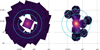 |
Fig. 1. FoV comparison between the exposure and background corrected 0.7 − 2 keV Chandra ACIS-I mosaic (left panel) and the exposure and vignetting corrected 0.7 − 7 keV Suzaku XIS mosaic (right panel) of Abell 1795. Images are to scale, but the smoothness and the color scales are not identical due to the different image sensitivities. The location of r500 and r200 is marked with the inner and outer circles, respectively, and on the right panel we also marked the Suzaku resolved point source regions with white. |
Particulars of the Chandra ACIS-I observations of Abell 1795.
First, we reprocessed the data with chandra_repro to apply the same calibration correction for each observation and to clean the ACIS particle background for VFAINT observations. Then, we removed observation periods with high background count rates caused by flares. Flare filtering was carried out using the deflare script with the lc_clean routine. We note that ACIS-I observations are not particularly sensitive to high background periods, and thus, the exposure times are not affected significantly. On average, < 8% of the exposure time was removed from the data.
Next, we constructed two sets of exposure maps for each observation to correct for vignetting and variations of quantum efficiency across the CCD. For tasks involving point sources, we assumed an absorbed power-law spectrum with a slope of Γ = 1.6, typical for active galactic nuclei (AGNs, e.g., Reeves & Turner 2000; Piconcelli et al. 2005). For the analysis of ICM emission, we assumed a phabs(apec) spectrum (in Xspec (Arnaud 1996) terminology) with a temperature of kT = 6.1 keV and an abundance of 0.2 solar. Assigning these spectral models analogously, we built spectrally weighted point spread function (PSF) maps for each observation with 90% encircled counts fraction (ECF).
Finally, individual observations were co-added to obtain a mosaic image of the cluster (Fig. 1, left panel). To this end, we used the merge_obs routine with the default “psfmerge” setting, which takes the minimum ECF at each pixel. In addition, to improve the cluster-background flux ratio of the observations, we applied an energy filter of 0.7 − 2 keV. Apart from the point source detection (Sect. 2.1.2), this filter was used in the analysis.
2.1.1. Background subtraction
The background subtraction in the point source analysis was carried out using local background regions. However, local background cannot be determined when probing ICM inhomogeneities due to the ICM’s extended nature. It is a common practice to model the ICM background using the ACIS blank-sky dataset. These observations, however, do not take into account the anisotropy of the cosmic X-ray background (CXB) and they resolve different CXB fractions due to different exposure times. Therefore, their use is not optimal for background-critical objects, such as clumps. Thus, when probing the ICM clumping, we relied on the ACIS stowed background dataset instead.
ACIS stowed background observations were collected with ACIS in the “stowed” position, namely, with the High Resolution Camera (HRC) in the focal plane. Thus, it only includes the instrumental background produced by the solar wind (Bartalucci et al. 2014), which has a constant spectral shape with varying normalization. Stowed background observations were taken between 2002 and 2012, while the outskirts of Abell 1795 were observed from 2015. Therefore, we utilized only the latest stowed data available in CALDB obtained between 2009 and 2011 with a total exposure time of ∼240.35 ks.
Stowed data reduction was carried out using the following steps. First, we applied VFAINT filtering then we reprocessed the data with acis_process_events. To account for the correct normalization between the stowed and cluster data, we followed the steps discussed in Hickox & Markevitch (2006). Specifically, we calculated normalization factors from the count rate ratios between the cluster observation and the corresponding stowed data in the 9.5 − 12 keV band, where the effective area of ACIS is negligible. Thus, with no astrophysical sources producing counts on the detector, the instrumental background remains the only contributor. In addition, we also corrected the readout artifacts of ACIS-I. We produced a readout background for each observation using the make_readout_bkg routine (Markevitch et al. 2000). The appropriate scaling was then applied in the same manner as for the stowed data. Finally, the sum of the scaled stowed and readout background was subtracted from each observation.
The X-ray background, in addition to the instrumental component, includes a sky component. It can be subdivided into the CXB produced by the unresolved population of AGN (Giacconi et al. 2001; Markevitch et al. 2003; Hickox & Markevitch 2006) and the Galactic foreground produced by the Local Hot Bubble (LHB) and the Galactic halo and disk (Snowden et al. 1995; Kuntz & Snowden 2000). These components are constant in time, and spatial variations of the foreground can be neglected within the field of view (FoV) of Abell 1795. Therefore, during imaging analyses, a constant sky background level is assumed.
2.1.2. Point source detection
Point sources in the field of Abell 1795 were identified with the CIAO wavdetect tool. We searched for point sources in the broad band (0.5 − 7 keV) on the total counts mosaic image. For the wavelet function, we specified pixel scales, employing the “ sequence” from
  to
to  , which selects both point-like and extended features. A signal threshold of < 10−8 was supplied for wavdetect to reduce the probability of spurious detections, and detection of faint ICM features, such as clumps. We set the “ellsigma” parameter to 5 to produce sufficiently large source cells. In most cases, this ensures the inclusion of ∼100% of the source counts, while residual source counts are not expected to significantly contribute to the ICM’s diffuse emission. The PSF information and effective area at each sky position were also provided for wavdetect. Finally, 1516 sources were identified. We used this source list for source exclusion when carrying out analyses described in Sects. 3.1 and 3.2.
To build the log N − log S plot for sources in the field of Abell 1795, point source detection was carried out separately in the soft band (0.5 − 2 keV) with the wavdetect parameters left unchanged. This run revealed 1137 sources.
2.2. Suzaku
Due to its low and stable instrumental background (non-X-ray background, NXB), we relied on data from the Suzaku X-ray Imaging Spectrometer (XIS) to probe the thermodynamic profiles of the cluster outskirts. The spectral analysis was refined by incorporating the Chandra point source list to bypass Suzaku’s low angular resolution, which causes unresolved point sources to add to the uncertainty of the measured properties of the diffuse emission. In addition, the surface brightness profile of Abell 1795 was also extracted from the Suzaku observations to compare it with the Chandra profile.
The analyzed Suzaku observations of Abell 1795 are listed in Table 2, while the full band mosaic is presented in the right panel of Fig. 1. We note that the Suzaku data does not provide full azimuthal coverage and has a smaller radial extent (∼30′) than the Chandra observations.
Particulars of the Suzaku XIS observations of Abell 1795.
The data reduction of XIS observations follows the procedure detailed in previous works (Simionescu et al. 2013; Urban et al. 2014; Zhu et al. 2021a). To summarize, we utilized the cleaned event files produced by the standard screening process available in the HEAsoft package (version 6.26)2 with all the recommended XIS screening criteria applied. Observation periods with low geomagnetic cut-off rigidity (COR ≤ 6 GV) were removed. The vignetting correction was carried out by utilizing ray-tracing simulations of a flat field image. Based on the solar proton flux curve measured by the WIND spacecraft’s solar wind experiment instrument, we also ensured that no contamination from the solar wind charge exchange (SWCX) during the clean exposure occurred.
For the imaging analysis, 0.7 − 2 keV images from XIS 0, 1, and 3 detectors were extracted along with the corresponding NXB obtained from the night-Earth data. To reduce the effect of systematic uncertainties caused by vignetting, a 30″ width region around the detector edges, and pixels with an effective area less than half of the on-axis value were removed from the background-subtracted images (Fig. 1, right panel). We then masked the point sources as detailed in Sects. 2.2.2 and 3.2.1.
Spectral extraction was carried out with XSELECT for five concentric annuli with widths of 5′ centered around the cluster and measured from 5′ to 30′, thereby excluding the cluster core. The Redistribution Matrix Files (RMF) and the Auxiliary Response Files (ARF) were produced in parallel with the mission-specific FTOOLS xisrmfgen and xisimarfgen commands, respectively. Finally, point sources were removed using three different approaches relying both on the Suzaku and the Chandra source list, as explained in Sect. 2.2.2. During the spectral fit of the ICM emission (Sect. 3.4), we accounted for the foreground, the CXB, and the NXB contribution, which we detail in the following subsections.
2.2.1. Modeling the foreground emission
The contribution of the LHB and Galactic components (Sect. 2.1.1) were modeled using the mission-specific X-Ray Background Tool (Sabol & Snowden 2019) on ROSAT All-sky Survey (RASS) diffuse background maps, which we downloaded for an annulus between 1.5r200 and 2.5r200 around Abell 1795. The extracted spectrum was fitted in Xspec with a tbabs × (apec + power − law)+apec model, where the unabsorbed and absorbed apec describes the LHB and the Galactic emission, respectively, while the absorbed power-law represents the fraction of the unresolved CXB in the RASS data. With the CXB parameters fixed at values adopted from Kuntz & Snowden (2000), we obtained plasma temperatures of 0.093 keV and 0.197 keV, and apec normalizations of 6.82 × 10⁻⁴ cm−5 and 1.39 × 10⁻³ cm−5 for the LHB and Galactic emission, respectively.
The ∼0.6 keV hot foreground component originating from the Galactic plane (Yoshino et al. 2009) is not important in the case of Abell 1795 because of the cluster’s relatively large galactic latitude (b = +77.1553). We confirmed this by adding a 0.6 keV apec component to our model, ultimately finding that its normalization could not be constrained, so the χ2 statistics did not improve.
2.2.2. Point source removal and modeling the CXB
The CXB contribution was estimated depending on the treatment of point sources. In the first approach (hereafter referred to as the first round or R1), only Suzaku resolved sources were removed from the data. These sources were identified on the broad-band Suzaku mosaic by wavdetect in a manner similar to that described in Sect. 2.1.2. The resulting source list collects 29 objects, which are marked on the right panel of Fig. 1. The flux of the remaining, unresolved sources was estimated from the point source excluded spectrum of the outermost annulus, where the ICM temperature is expected to drop below 2.5 keV. We fit the spectra in XSpec with a power-law in the 4 − 7 keV band, where the CXB emission dominates, and obtained a best-fit photon index of Γ = 1.5 and a normalization of 1 × 10⁻³ photons keV−1 cm−2 s−1 at 1 keV.
In the second round (R2) of spectral extraction, we accounted for the limits on Suzaku’s angular resolution by extending the R1 point source list with the Chandra broad-band source catalog (Sect. 2.1.2) down to a 2 − 8 keV flux threshold of ∼1.2 × 10⁻¹⁴ erg cm−2 s−1. Based on the hard band log N − log S plot built in the same way as described in Sect. 3.3, 95% of the sources above this flux threshold are resolved in the current set of Chandra data. To account for the broader PSF of Suzaku, the radius of each Chandra source was increased to 1′ as a first approximation. We note that the spatial resolution of XIS detectors is ∼1.8′. For completeness, we also added sources that were identified separately on those calibration observations that cover the data gap in Chandra data (Fig. 1, left panel). This step was needed because of the partial overlap between the Suzaku pointings and the Chandra data gap. Processing and merging of the calibration observations were carried out following the standard CIAO procedure, while the point source detection was identical to that described in Sect. 2.1.2. Considering the extended source list, the reduced CXB flux of R2 was estimated from the cluster’s log N − log S plot (Sect. 3.3) using CXBTools (Mernier et al. 2015; de Plaa 2017). This yielded a CXB flux of 1.14 × 10⁻¹¹ erg cm−2 s−1 deg−2 in the 2 − 8 keV band. To this flux, we added the 50% of the total 2 − 8 keV flux, 1.55 × 10⁻¹³ erg cm−2 s−1 deg−2, of the removed Chandra sources to account for excess point source emission beyond source radii of 1′, which is below XIS’s angular resolution. This approach was optimized to secure a FoV area that is sufficient for spectral extraction. From the estimated CXB flux, a power-law photon index of Γ = 1.4 and normalization of 8.87 × 10⁻⁴ photons keV−1 cm−2 s at 1 keV were obtained.
In the third round (R3) of spectral extraction, we probed the influence of ICM clumping, so we further extended the R2 source list with the clump candidate regions C1, C2, C6, C8, C10, and C12. The rest of the candidates are either not covered by Suzaku or were already removed in R2 due to the overlap with a point source (Fig. 2). Since the clump candidates’ contribution to the total resolved source flux is negligible, and these sources are essentially not part of the CXB, we used the R2 CXB parameters here.
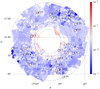 |
Fig. 2. Adaptively binned image of Abell 1795 outskirts in the 0.7 − 2 keV energy band. The image is instrumental background- and exposure-corrected. Each bin has a S/N of ≳3, and a surface brightness value indicated by the colorbar in photon cm−2 s−1 pixel−1 units. Small white ellipses scattered throughout the field represent excluded point sources. We used this image to measure the surface brightness distribution within each annulus (dashed-line circles) and to isolate outliers that may originate from ICM inhomogeneities. Outlier positions are shown with small circles marked from C1 to C24 (for the actual size and shape of the outliers, see Fig. 4). |
2.2.3. Modeling the particle background
The NXB is produced by charged particles and γ-ray photons hitting the detector. Its spectrum was extracted with xisnxbgen from the weighted, integrated night-Earth observations taken in a time window of ±150 days of the Abell 1795 observations. Instead of directly subtracting it from the cluster data, we tailored them to our observations by modeling their spectra. For more details, we refer to Zhu et al. (2021a).
Because of their different designs, front-illuminated (FI) CCDs (XIS 0 and XIS 3) and the back-illuminated (BI) CCD (XIS 1) have different sensitivities to the NXB (Hall et al. 2007; Tawa et al. 2008), resulting in different spectral shapes. Accordingly, we modeled the FI NXB spectra with a power-law representing the continuum, to which we added nine Gaussian emission lines representing the instrumental lines between 1 keV and 12 keV. In the BI XIS spectral model, we added another broad Gaussian component to account for the continuum bump above 7 keV.
We fit the FI and BI NXB models to the convolution of the NXB and a diagonal RMF for each observation. During the fit, we fixed the line centroid parameter, adopted from Tawa et al. (2008), of those instrumental lines, which lie above 5 keV, where the contribution of ICM emission of the cluster outskirts is negligible. Finally, the NXB normalization factor was constrained during spectral modeling from the 7 − 12 keV source spectra based on similar principles as discussed in Sect. 2.1.1.
2.2.4. Systematic uncertainties
Spatial variations across the Suzaku FoV might be present in the foreground X-ray emission, as well as in the CXB (called the cosmic variance), and our spectroscopic measurements are the subject of the corresponding systematic uncertainties. A coarse measure for the uncertainty is provided here for both background components and demonstrated on the projected temperature profile in Appendix B.
The spatial variation of the diffuse galactic X-ray emission was assessed from RASS spectra extracted in four directions around Abell 1795 beyond 1.5r200 within 2° diameter circles. We fit each spectra with a tbabs × apec model and found a 25% variance in the best-fit normalizations.
The σ2 cosmic variance in the expected  brightness of unresolved X-ray point sources with flux S < Sexcl over a given Ω solid angle can be expressed, following Bautz et al. (2009), as:
where dN/dS is the differential number of AGN per unit solid angle and flux, which we approximated with a broken power law with parameters adopted from Lehmer et al. (2012). For Sexcl we adopted the limiting flux of R1 (∼2.6 × 10⁻¹⁴ erg cm−2 s−1) and R2 (R3) (1.2 × 10⁻¹⁴ erg cm−2 s−1, Sect. 2.2.2). Over the 5′−30′ radial range, we found an average σ/B relative cosmic variance of ∼6.5% and ∼5.1% in R1 and R2 (R3), respectively. As expected, excluding more of the brightest point sources, the primary sources of spatial variations, scales down the cosmic variance. However, it caused only a modest improvement from R1 to R2 (R3). It is the result of the relatively large limiting flux applied for R2 (Sect. 2.2.2), which was optimized so that spectral extraction from the outermost annulus remains feasible given the limited coverage and spatial resolution of Suzaku, which, in turn, yielded only modest difference in the limiting fluxes between R1 and R2.
3. Results
3.1. Identifying ICM inhomogeneities
A robust method for identifying ICM inhomogeneities was presented by Zhuravleva et al. (2013). Based on this, the gas density of a perfectly homogeneous ICM should follow a log-normal distribution measured within a narrow spherical shell. In the presence of gas inhomogeneities, however, a “high-density tail” emerges in the distribution, distorting its log-normal shape. As a consequence, the mean and median of the distribution separate, with the median staying around the peak while the mean shifts to higher densities. Suggested by numerical simulations (e.g., Kawahara et al. 2008; Zhuravleva et al. 2013; Khedekar et al. 2013; Rasia et al. 2014), the same applies to the surface brightness or the flux (note: the ICM’s X-ray emission scales with the square of gas density), which are also log-normally distributed. The insensitivity of the surface brightness median to ICM inhomogeneities was also demonstrated by Eckert et al. (2015). Instead of relying on the gas density, which cannot be measured directly, we searched for ICM inhomogeneities in the surface brightness distribution of the cluster.
To measure the surface brightness distribution in a radial range, we first binned the total counts mosaic image using the contbin algorithm (Sanders 2006). The algorithm is based on an adaptive binning technique and divides the input image into bins having approximately the same signal-to-noise ratio (S/N). For the S/N calculation, we supplied the stowed background data for contbin, and set the S/N threshold to > 3. Point sources were masked both from the input and background mosaic. Since ICM inhomogeneities are expected to concentrate on the outskirts, the cluster core was also masked to reduce computational time. With these settings, the cluster core-excluded mosaic was divided into 1132 irregular-shaped and unequal-sized bins by contbin. The smallest bins have a scale of ≲1″ × 1″, which corresponds to 1.2 × 1.2 kpc at the distance of Abell 1795. The resulting binmap was then applied to the background- and exposure-corrected image, which was then divided by concentric annuli (Fig. 2), and the surface brightness in each bin was measured. The annuli were defined to have a logarithmically increasing radius so that the number of enclosed bins is sufficiently large to build the surface brightness distribution, even at the outermost annulus with the lowest surface brightness and thus, the lowest number of bins.
In Fig. 3, we present the surface brightness distributions between ∼13′ (0.5r200) and ∼42.5′ (≈1.6r200). At larger cluster radii, the “bulk” (i.e., log-normal) and “high-surface-brightness tail” components of the histograms are clearly distinguishable. Accordingly, while the median surface brightness coincides well with the peak, the mean is shifted towards high surface brightness, implying more weight in the right tail of the distribution. To quantify this asymmetry, we calculated the Fisher-Pearson coefficient of skewness of the distributions. The mean, median, and skewness, along with the annulus properties, are listed in Table 3. The error bars represent 1σ bootstrap confidence intervals with 105 resamplings. We found that the skewness is positive in each annulus and shows an increasing tendency with radius.
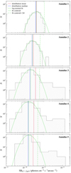 |
Fig. 3. 0.7 − 2 keV surface brightness distribution of the ICM in the outskirts of Abell 1795 obtained in 5 annuli. The annuli extend out to ∼42.5′ as listed in Table 3. Overall, the median surface brightness coincides with the peak of the distribution, but the mean, especially at larger radii, is shifted towards high values, which suggests the presence of unresolved gas inhomogeneities (Zhuravleva et al. 2013). We selected the > + 2σ outliers of the log-normal fit within each annulus, which resulted in a total of 24 sources to form our list of clump candidates. |
Surface brightness distribution parameters from the adaptively binned image in five annuli.
We fit each annulus distribution with a log-normal function and then, using the σ standard deviation of the best-fit function, we selected > + 2σ outliers from the fit centroid (listed in Table 3) and localized them on the image. After merging adjacent outlier bins, we identified 24 clump candidates. Their properties are reported in Table 4, and their spatial distribution is displayed in Fig. 2. The significance of multi-bin clump candidates was calculated from the overall surface brightness measured within the merged bins. An increasing trend with the radius is apparent in the frequency of the sources, with a higher projected concentration at the western hemisphere of the cluster. Both the spatial distribution of individual sources and the skewness suggest that the effect of ICM inhomogeneities on the measured surface brightness is more significant at larger radii, in accordance with simulation predictions.
Clump candidate properties.
3.1.1. Optical counterparts
Figure 4 shows cutout images centered around the clump candidates in the 0.7 − 2 keV band. Most candidates are connected with one or multiple wavdetect sources, which are surrounded by or adjacent to the clump candidate region, suggesting that their emission may originate from the same X-ray source. It might also imply that the candidates are not genuine clumps. To uncover the nature of clump candidates and explore their surroundings, we searched for optical counterparts in the Sloan Digital Sky Survey (SDSS). We collected images from SDSS Data Release 16 for each candidate and the catalog of galaxies and their photometric properties in the surroundings. Figure 4 shows SDSS r-band images presenting the same FoV as the Chandra cutout images. We found that 21 of 24 candidates coincide with multiple sources, while 1 candidate (C22) coincides with only one SDSS source. Clump candidates C13 and C20 remained with no co-spatial SDSS galaxies.
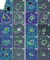 |
Fig. 4. Chandra 0.7 − 2 keV (left panel, color images) and SDSS r-band cutout images (right panel, greyscale images) showing the individual clump candidates (white, irregular-shaped regions) and their environment within a 200″ × 200″ area. The Chandra images are smoothed with a Gaussian of a radius of 6 to accentuate the X-ray excess. Filled black ellipses represent excluded wavdetect sources, while the filled red circle at the bottom left of each Chandra image marks the local minimum size of PSF. As most of the clump candidates overlap with multiple SDSS galaxies (green circles), possible physical connections must be addressed to isolate genuine clumps (Sects. 3.1.1 and Appendix A). |
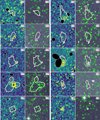 |
Fig. 4. continued. |
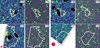 |
Fig. 4. continued. |
To test whether the X-ray emission of clump candidates originates from an overlapping SDSS galaxy, we executed an X-ray flux comparison between the sources. Based on visual inspection of X-ray and optical images, we selected only those galaxies for this test that are associated with excess X-ray emission within (or, in certain cases, around) the corresponding clump candidate region. We set this criterion to keep our results reasonable in cases where the number of overlapping galaxies is too high (e.g., C17) or where galaxies are obviously not X-ray emitters (e.g., C15). Candidates with a co-spatial relation with a background galaxy cluster or group or that are located near the detector edge have not been subjected to this analysis. Thus, we selected a total of 26 galaxies from SDSS, which may be associated with clump candidates C1, C3 − 8, C10, C14, C16, C18 − 19, and C21 − 22.
When estimating the expected X-ray flux of galaxies, we assessed the contribution of the unresolved population of low-mass X-ray binaries (LMXBs) and, for galaxies with a stellar mass of M* > 7 × 10¹⁰ M⊙, the diffuse emission of the hot interstellar medium (ISM). Below this particular mass threshold, we do not expect the galaxies to host luminous X-ray halos according to local scaling relations (e.g., Bogdán & Gilfanov 2011; Kim & Fabbiano 2013; Kim et al. 2019). We did not consider the X-ray emission from AGN and the high-mass X-ray binary population. The latter is only significant for galaxies with star formation rate (SFR) ≳1 (Grimm et al. 2003), and, although the SFR of the selected galaxies is unknown, their average u − r = 2.14 color index indicates that the galaxy sample consists mainly of early-type galaxies (Strateva et al. 2001), which typically exhibit low SFR.
The stellar mass of the galaxies was derived from SDSS broadband photometric data (r magnitudes and u − r color indices) and photometric redshift using the stellar mass-to-light ratio (Bell et al. 2003). We found that only about one-third of the galaxies are massive enough to host an X-ray luminous halo. Based on the derived stellar masses, the LMXB X-ray luminosity contribution was estimated using the  scaling relation (Gilfanov 2004) and the diffuse X-ray emission luminosity was estimated from the
  scaling relation (Kim et al. 2019). The resulting X-ray luminosities were converted into 0.7 − 2 keV fluxes and added up within each clump candidate. For the conversion of LMXB luminosities, we assumed a power-law model with a slope of Γ = 1.56 (Irwin et al. 2003), and for the ISM, an apec model with kT = 0.5 keV (e.g., Bogdán & Gilfanov 2011; Goulding et al. 2016).
Similarly, the measured stowed background subtracted X-ray flux was added up within each clump candidate region, corrected for the sky background, then converted from photon flux to energy flux units. For the conversion, we assumed an absorbed apec with kT = 1 keV, describing the diffuse emission of cluster outskirts beyond r200. We note that the source of X-ray emission in clump candidates is uncertain, but assuming a power-law model, for instance, would lead to a ∼19% increment in the conversion factor. Our results are reported in Appendix A only for those sources where flux comparison was conclusive.
3.1.2. Hardness ratio
To further assess the source of X-ray emission in clump candidates, we gathered their rough spectral properties by measuring their hardness ratios. The hardness ratio is defined as  , where A and B are the exposure corrected counts measured in the 2 − 7 keV and 0.5 − 1.5 keV bands, respectively. A hardness ratio of HR ≈ 0 is consistent with a power-law spectrum with a slope of Γ = 1.4 − 1.7, while HR ≈ −0.5 and HR ≈ −0.8 characterize an apec spectra with kT = 2 keV and kT = 1 keV, respectively. Thus, hardness ratios provide the means to distinguish between the emission of a background AGN and thermal emission from diffuse gas at or below the temperature of cluster outskirts. We note that clumps are predicted to have kTclump < kTICM (Vazza et al. 2013), and kTICM ≃ 2 keV between r500 and r200 for Abell 1795.
Due to the Poissonian distribution of counts, we calculated the hardness ratios and the associated confidence limits using the Bayesian Estimation of Hardness Ratios (BEHR) code (Park et al. 2006). We defined a local background around each clump candidate as an annulus with a width of 0.5′ and the inner radius defined as the radius of the smallest fitting circle around the irregular-shaped source. Source and background counts were extracted from exposure-corrected images with wavdetect sources excluded, then fed to BEHR. The obtained hardness ratios are listed in Table 4; they could not be constrained for 6 out of 24 clump candidates.
3.2. Surface brightness profile
3.2.1. Azimuthally averaged surface brightness profiles
Extraction and fitting of the Chandra and Suzaku surface brightness profiles of Abell 1795 were carried out using the PROFFIT software package (Eckert et al. 2011). The azimuthally averaged profiles were constructed considering only the outskirts of Abell 1795 beyond a radius of ∼11.25′ (∼ 0.8 Mpc).
To generate the surface brightness profiles of the diffuse emission, we excluded bright point sources from the extraction regions. Because the Chandra and Suzaku observations of Abell 1795 have different source detection sensitivities, it is important to define a specific limiting flux above which point sources are removed from both data sets. We used the broad-band source list identified by wavdetect (Sect. 2.1.2); for Suzaku, we tailored it to its larger PSF (as described in Sect. 2.2.2) and applied a uniform photon flux threshold of 2 × 10⁻⁶ photon cm−2 s−1, which corresponds to an energy flux of ∼5.8 × 10⁻¹⁵ erg cm−2 s−1 for both telescopes. We found that 68% of the Chandra detected sources lie above this threshold.
When building the profile, we binned the 0.7 − 2 keV photon counts within > 60″ (for Suzaku within > 160″) width concentric annuli centered on the cluster’s X-ray peak (J2000(RA, Dec) = (207.2194, 26.5920) in FK5 coordinates), applying logarithmic binning. The instrumental background (stowed background for Chandra, and NXB for Suzaku) and exposure maps were also taken into account.
We fit the obtained Chandra and Suzaku profiles separately with a power-law model of Sx ∝ r−α + B, where B represents the sky background constant. We note that the power-law model provides a better description for the outskirts compared to the standard β-model due to the strong coupling between the β parameter and the core radius (Mohr et al. 1999), which falls outside the fitting region, and therefore could not be constrained.
In Fig. 5, we display the resulting background subtracted surface brightness profiles and the best-fit models in units of erg s−1 cm−2 deg−2 to allow a direct comparison between the two datasets. For the photon flux to energy flux conversion, we assumed an apec model with kT = 2 keV and with 0.2 solar abundance. We also display the instrumental and sky background profiles to demonstrate their significant contribution to the outskirts. Note the factor of ∼4 difference between the level of Chandra’s stowed background and Suzaku’s NXB and the dominant contribution of the stowed background to the surface brightness beyond ∼0.5r200.
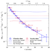 |
Fig. 5. 0.7 − 2 keV background-subtracted azimuthally averaged surface brightness profiles of Abell 1795 outskirts measured with Chandra and Suzaku with the corresponding best-fit power-law models overplotted. The background components are also shown. Point sources were removed down to a photon flux of 2 × 10⁻⁶ photons cm−2 s−1 from both datasets and the elevated Suzaku sky background level reflects the excess emission from point sources whose PSF is broader than the corresponding source region. |
The two profiles are in agreement with a best-fit power-law exponent of 4.05 ± 0.14 and 4.18 ± 0.19 for Chandra and Suzaku, respectively. These relatively high exponents represent a steep fall in the cluster surface brightness beyond 0.4 r200. We emphasize that this degree of agreement between the Chandra and Suzaku extracted profiles is the consequence of the coordinated source removal procedure, which we explain further in Sect. 4.3.
3.2.2. Azimuthal surface brightness profiles
Azimuthal variations in the structure of the ICM (and so in the surface brightness profile) may be present even in dynamically relaxed systems (e.g. Urban et al. 2011, 2014; Eckert et al. 2012). In Abell 1795, Bautz et al. (2009) reported excess emission in the northern direction based on 0.5 − 2 keV Suzaku data, with an apparent peak near 23′. To probe asymmetries in the cluster’s diffuse emission with Chandra, we built the 0.7 − 2 keV surface brightness profiles from circular wedges toward the north, south, east, and west directions with opening angles of 90°.
The source removal in this case was carried out without the limiting flux threshold applied in Sect. 3.2.1, namely, considering the full list of broad-band wavdetect sources. To achieve signal-to-noise ratios comparable to those obtained for the azimuthally averaged profile, we increased the bin width to > 160″. Because of the uneven azimuthal coverage (Fig. 1), we introduced a uniform fitting range of 7′−31′ and we fit the profiles within this range in a way identical to that applied for the azimuthally averaged profile (Sect. 3.2.1). We note that the fitted sky background constant has no effect on the obtained power-law exponents, therefore, we did not subtract its contribution for plotting purposes. The obtained sky background-included profiles are displayed in Fig. 6 with the best-fit power-law models. The corresponding power-law exponents are 4.50 ± 0.20, 3.99 ± 0.17, 2.78 ± 0.12, and 3.29 ± 0.15 for north, south, east, and west, respectively.
 |
Fig. 6. 0.7 − 2 keV surface brightness profile of Abell 1795 outskirts extracted from Chandra data in four different directions. Azimuthal variations relative to the average profile are displayed in the bottom panel. |
We found that the excess brightness from the north between r500 and r200 recorded by Bautz et al. (2009) in the Suzaku data is not present in the Chandra-extracted profile. This fluctuation likely comes from a point source located at 207.26°, 26.98° in the RA/Dec plane, which exhibits an extremely broad PSF resulting in an apparent source radius of ∼3′ in the Suzaku observations. Although this point source was successfully identified by wavdetect, the size of the source region required manual adjustment when removing it from the Suzaku data for the azimuthally averaged surface brightness profile. We emphasize that the Suzaku profile indeed displayed an excess at ∼25′ without this adjustment.
In the bottom panel of Fig. 6, we present the azimuthal variations in the level of the surface brightness in the four extraction directions. Although the profiles exhibit a significant scatter, an obvious enhancement toward the western direction is seen beyond ∼18′ with an average significance of 4.2σ. A possible explanation for this deviation is given in Sect. 4.4.
3.3. The log N − log Splot
The log N − log S plot accounts for the cumulative number of sources (N) as a function of source flux (S) per square degree within a selected field and includes mostly point sources, namely, AGN. Galaxies become significant contributors only in the soft X-ray band at ≲10−17 erg cm−2 s−1 (Luo et al. 2017), which is below the detection limit of the present analysis.
We built the log N − log S plot, incorporating all sources detected on the 0.5 − 2 keV Abell 1795 mosaic, inclusive of the central pointing, with a detection significance of ≥3σ (∼94% of the wavdetect identified sources). Source fluxes were calculated using the srcflux CIAO tool assuming an absorbed power-law spectrum with a photon index of Γ = 1.6. Local background annuli were defined with roi in consideration of overlapping regions and with the inner background radius of twice the source radius. To accurately account for the high variability of the FWHM across the FoV, the PSF fraction in each source and background region was computed with marx simulations. Finally, for the log N − log S plot, we adopted the sources’ intrinsic flux, that is, the unabsorbed model flux estimates based on the power-law assumption.
For the area normalization, that is, to specify the solid angle surveyed as a function of limiting flux, we constructed a sky coverage histogram in the soft band. The input limiting sensitivity map for this was created for the merged data with the lim_sens CIAO tool, assuming a Γ = 1.6 power law model. This sensitivity map determines the 3σ limiting flux variations across the FoV due to the spatial variations of the PSF, effective exposure and background level, with the inclusion of the sky, instrumental, and the ICM background components.
We present the 0.5 − 2 keV log N − log S plot for the Abell 1795 field in Fig. 7 compared to the results from the 7 Ms Chandra Deep Field South (CDF-S) data (Luo et al. 2017). A minimum flux threshold of 5.4 × 10⁻¹⁶ erg cm−2 s−1, adjusted to a minimum survey area of 5% of the FoV, was applied to reflect the high uncertainties at low sky coverage, while a maximum flux threshold of 7.0 × 10⁻¹⁴ erg cm−2 s−1 was also introduced to correct for the lowest exposure survey areas. Within 1σ uncertainty, the source number counts in the field of Abell 1795 agree with those of the CDF−S with only minor discrepancies at the high-flux-tail (source deficit) and at ∼10−14 erg cm−2 s−1 (source excess).
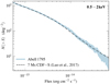 |
Fig. 7. Log N − log S plot for the sources detected in the Abell 1795 field (shaded curve with 1σ uncertainty) and in the 7 Ms Chandra Deep Field South (Luo et al. 2017). Despite the excess in the number of Abell 1795 field sources seen at ∼10−14 erg cm−2 s−1, which can be attributed to the cosmic variance, the distributions are in good agreement at fluxes below ∼6 × 10⁻¹⁴ erg cm−2 s−1. No excess can be explicitly attributed to unidentified clumps among wavdetect sources. |
Besides the CDF-S field, we compared the present results with other surveys to test the significance of the excess, which is a potential contribution from ICM clumps. Specifically, the cumulative source number counts at S > 10−14 erg cm−2 s−1 exhibit a scatter of ∼45 source counts in a sky area of one square degree based on the Lockman Hole surveyed by XMM-Newton (Hasinger et al. 2001), a combination of six different surveys performed with ROSAT, Chandra, and XMM-Newton (Moretti et al. 2003), and the XMM−COSMOS field (Cappelluti et al. 2007). As this scatter surpasses the excess seen in the Abell 1795 data, we attribute this source excess to cosmic variance.
3.4. Thermodynamic profiles
The radial profiles of the ICM’s thermodynamic properties were derived from spectral analysis of the Suzaku data in a way identical to that described in Zhu et al. (2023). We grouped the spectral counts so that each channel contains at least one count, then modeled the XIS spectra with Xspec. The parameter estimation was carried out using the C-statistics due to the Poissonian distribution of the data. We described the ICM emission as an absorbed, collisionally ionized thermal plasma with a tbabs × apec model and the background contribution to the detected X-ray signal is considered as explained in Sects. 2.2.1 and 2.2.3. The spectral fitting was carried out in three rounds (R1 − 3, see Sect. 2.2.2) in five radial bins enclosing a 5′−30′ annulus centered around the cluster. Based on Werner et al. (2013) and Urban et al. (2017), we fixed the abundance at Z = 0.3 Z⊙ beyond r500, where Z⊙ refers to the value presented in Lodders et al. (2009).
The ICM emission we measure this way is superposed from 3D shells along the line of sight, meaning that the cluster properties derived from the 2D spectra (e.g. temperature, Fig. 8) suffer from projection effects. To correct for this effect, we deprojected the 2D spectra using Xspec’s model-dependent PROJCT tool assuming spherical symmetry. The ICM emission in each shell was modeled with an absorbed apec. For background modeling, we used a smoothed NXB generated with fakeit for the correct propagation of the uncertainties in the NXB spectrum.
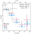 |
Fig. 8. Projected temperature profiles of the Abell 1795 cluster outskirts from three rounds (R1−3) of spectral extraction. In the R1 data, only the Suzaku resolved point sources, while from the R2 data, all point sources down to a flux of 5.8 × 10⁻¹⁵ erg cm−2 s−1 were removed. The R3 profile, on top of that, accounts for the effect of the resolved clump candidates, which is insignificant. For comparison, we included three additional profiles from previous works. |
We obtained the temperature profiles directly from the best-fit apec models, and derived the electron density from the deprojected apec normalization, then calculated the plasma pressure and entropy from the deprojected properties. The outermost data points of cluster properties derived from deprojection at 25′−30′ might be biased by significant systematic uncertainties, likely caused by non-zero ICM emission beyond 30′ or by morphological asymmetries (Sect. 4.4); thus, they might be incorrect. In Fig. 9, these measurements are drawn with dashed lines but are not considered when discussing the results.
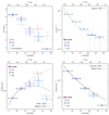 |
Fig. 9. Deprojected profiles of the cluster outskirts with R1−3 denoting the deprojected equivalents of the profiles shown in Fig. 8 (Sect. 2.2.2). The outermost data points, shown with dashed lines, exhibit large uncertainties introduced with the deprojection. Top left: comparison between the deprojected and the projected temperature profiles. Top right: electron density profiles overplotted with ROSAT measurements of the same cluster by Eckert et al. (2013). Bottom left: entropy profiles compared with the profile of Pratt et al. (2010), which models a galaxy cluster formed by gravitational collapse with no additional heating or cooling and with the analytic function of Walker et al. (2012) fitted on a sample of Suzaku observed clusters. Bottom right: pressure profile overplotted with the best-fit models of Arnaud et al. (2010) and the Planck Collaboration Int. V (2013). |
3.4.1. Temperature profile
Figure 8 shows projected gas temperature profiles for each run. We emphasize that the present dataset, extending beyond r200, probes the outskirts at their lowest-surface-brightness regime that has so far been only poorly explored. Beyond r200, the R1 profile becomes statistically unconstrained, while the R2 and R3 profiles flatten at ≳2 keV. A slight tendency of increasing temperature difference with increasing radii can also be observed between the R1 and R2–R3 profiles. We find that the R2 and R3 profiles are in agreement, suggesting no influence on the projected temperature from the resolved fraction of clump candidates at the scales of the present study. However, we note that systematic effects, albeit relatively low, introduce additional uncertainties, which we discuss in Appendix B.
In Fig. 8, we also present results obtained from Chandra observations (Vikhlinin et al. 2005), from XMM-Newton observations (Snowden et al. 2008) and from Suzaku observations of the northern cluster region (Bautz et al. 2009). We note that the Suzaku observations of Abell 1795 point in multiple directions, but in the work of Bautz et al. (2009), only the northern temperature measurements extend beyond r500. Within the error bars, the present results are in agreement with those obtained from XMM-Newton and from the former Suzaku analysis, while the measurements from Chandra show, on average, higher temperatures within r500. We also emphasize that the present Suzaku results are not identical to those obtained by Bautz et al. (2009), not only because of the different azimuthal coverage but also because the changes in Suzaku calibration and apec code affect the best-fit temperature determination.
We show the deprojected temperature profiles obtained for R1−3 in the top left panel of Fig. 9. The R1–3 plasma temperatures show a gradual decrease with radius reaching 2 − 3 keV at < r200, and the effect of clump candidates is only marginal.
3.4.2. Electron density profile
Densities were derived from the emission measure (EM = ∫nenH dV) contained in the best-fit apec model normalization:
![$$ \begin{aligned} \mathrm{Norm} = \frac{10^{-14}}{4 \pi [D_{\mathrm{A} } (1+z)]^2} \int n_{\mathrm{e} } n_{\mathrm{H} }\, \mathrm{d}V ,\end{aligned} $$](/articles/aa/full_html/2023/10/aa47201-23/aa47201-23-eq37.gif)
where DA is the angular distance to the Abell 1795 cluster, and dV is the volume element, while ne and nH are the electron and hydrogen number densities, respectively. We assumed a fully ionized plasma, where ne = 1.2nH. The emitting volume was expressed as  , and the correction for FoV irregularities was handled by the ARF information.
We compare the electron number density distribution in the top right panel of Fig. 9 with that obtained by Eckert et al. (2013) from ROSAT observations of the same cluster. We note that the latter one follows the isothermal β-model with β ≈ 2/3, which is the canonical value for large clusters (Jones & Forman 1984). Both the different Suzaku runs (R1–3) and the ROSAT profiles are in agreement with each other suggesting a gradual density decrease with radius. Although ROSAT observations extend beyond r200, most of the > 0.8r200 data points exhibit large errorbars, while the present data confirm ne to be ∼5 × 10⁻⁵ cm−3 at ∼(0.8 − 1)r200.
3.4.3. Entropy profile
The radial distribution of entropy, defined as  , is presented in the bottom left panel of Fig. 9. The observed profile is compared with that predicted assuming pure gravitational heating, where the entropy is expected to follow a power-law relation with K ∼ r1.1 (Voit et al. 2005). Expressed with the dimensionless entropy, the profile follows:

where  is the characteristic entropy (Voit et al. 2005; Pratt et al. 2010), M500 = 6 × 10¹⁴ M⊙ is the cluster mass within r500 (Vikhlinin et al. 2006), the fb baryon fraction is taken to be 0.15, and
  is the ratio of the Hubble constant at z with its z = 0 value. The pure gravitational collapse of a galaxy cluster, however, may be disrupted by non-gravitational processes (e.g., AGN feedback and sloshing close to the cluster core or clumping and accretion shocks at the outskirts), which modify the above picture. Therefore, we compare our results with the analytical function yielded for a sample of cool core galaxy cluster outskirts (r > 0.2r200) at z ≤ 0.25 (including Abell 1795) by Walker et al. (2012):
with  . This formula predicts an entropy flattening and turnover at ≳0.4 r200.
The R2 − 3 profiles run between the two model curves and feature no turnover points. The positive radial entropy gradient suggests that the ICM is convectively stable. However, the measured profile is still lower than the theoretical curve calculated under the assumption of pure gravitational heating. A possible explanation for this deviation is presented in Sect. 4.5.
Interestingly, in contrast to Abell 1795, the entropy profile of Abell 133 shows a definite flattening following the Walker profile, even upon the removal of clump candidates (R3 profile). For details, refer to the companion paper of Zhu et al. (2023).
3.4.4. Pressure profile
The P = nekT radial pressure profile is shown in the bottom right panel of Fig. 9, overplotted with the best-fit models of Arnaud et al. (2010) and the Planck Collaboration Int. V (2013), both parametrizing the generalized form of the pressure profile proposed by Nagai et al. (2007), as follows:
![$$ \begin{aligned} \frac{P(r)}{P_{500}} = \frac{P_0}{ (c_{500}x)^{\gamma } \, [1+(c_{500}x)^{\alpha }]^{(\beta -\gamma )/\alpha }} ,\end{aligned} $$](/articles/aa/full_html/2023/10/aa47201-23/aa47201-23-eq45.gif)
where ![$ P_{500} = 1.65 \times 10^{-3} \, E(z)^{\frac {8} {3}} \left [ \frac{M_{500}}{3 \times 10^{14} h_{70}^{-1}\,{M}_{\odot}}\right ]^{\frac {2} {3}} h_{70}^2\,\mathrm{keV}\,\mathrm{cm}^{-3} $](/articles/aa/full_html/2023/10/aa47201-23/aa47201-23-eq46.gif) is the characteristic pressure which scales with the cluster mass purely based on gravitation, x = r/r500, c500 is the concentration parameter at r500, and α, β, and γ are the profile slopes in the intermediate, outer and central regions, respectively. From a sample of z < 0.2 clusters explored within 0.6r200 with XMM-Newton, Arnaud et al. (2010) obtained a best-fit parameter set of [P0, c500, α, β, γ]=[8.403, 1.177, 1.0510, 5.4905, 0.3081], while from the sample of Planck clusters explored at 0.02r500 < r < 3r500, the Planck Collaboration Int. V (2013) obtained [P0, c500, α, β, γ]=[6.41, 1.81, 1.33, 4.13, 0.31], yielding a slightly flatter profile. The present measurements, overall, are consistent with the models, although the R3 data point above ∼0.75r200 might be indicative of a steeper pressure drop in the outskirts compared to the Planck baseline profile.
is the characteristic pressure which scales with the cluster mass purely based on gravitation, x = r/r500, c500 is the concentration parameter at r500, and α, β, and γ are the profile slopes in the intermediate, outer and central regions, respectively. From a sample of z < 0.2 clusters explored within 0.6r200 with XMM-Newton, Arnaud et al. (2010) obtained a best-fit parameter set of [P0, c500, α, β, γ]=[8.403, 1.177, 1.0510, 5.4905, 0.3081], while from the sample of Planck clusters explored at 0.02r500 < r < 3r500, the Planck Collaboration Int. V (2013) obtained [P0, c500, α, β, γ]=[6.41, 1.81, 1.33, 4.13, 0.31], yielding a slightly flatter profile. The present measurements, overall, are consistent with the models, although the R3 data point above ∼0.75r200 might be indicative of a steeper pressure drop in the outskirts compared to the Planck baseline profile.
4. Discussion
4.1. Emissivity bias
Almost all clump candidates reported in Appendix A are associated with background objects projected at Abell 1795 (Table 4). Although these are not genuine clumps, their effect can mimic clumps seen in simulations. In Sect. 3.4, we compare the thermodynamic profiles with clump candidates included (R2) and removed (R3), but no influence on the overall picture was found.
More generally, the effect of clump candidates can be assessed, following Eckert et al. (2015), by calculating the ratio between the mean and the median of the surface brightness distribution (Fig. 3). The bX = SBmean/SBmedian emissivity bias profile obtained this way is displayed in Fig. 10 and listed in Table 3 with the error bars marking 1σ bootstrap confidence intervals from 105 resamplings. We emphasize that bX is a purely observational quantity that is strongly influenced by the contribution of the sky background and projection effects. A perfectly uniform ICM is characterized by bX = 1, when these effects are not present.
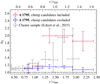 |
Fig. 10. Radial variation of the bX emissivity bias when each clump candidate is included or excluded, compared to the results from the ROSAT sample of 31 galaxy clusters (Eckert et al. 2015). The 24 clump candidates, although being not genuine clumps, cause an increased level of bias above ∼0.8 r200 in Abell 1795. When each clump candidate is excluded, the profile flattens at bX ≥ 1. Note: bX is subject to projection effects and influenced by the sky background contribution, which exhibit very different levels for the Chandra and ROSAT data sets. |
In Fig. 10, we compare the emissivity bias in the outskirts of Abell 1795 with the average measurements of Eckert et al. (2015) for a sample of 31 ROSAT/PSPC observed galaxy clusters. The Abell 1795 profile shows a sharp jump at ∼0.8r200 followed by a plateau with bX ∼ 2. In contrast, the ROSAT sample, which is characterized by large uncertainties, features a gradual increase with radius. Upon the removal of the resolved clump candidates from the Abell 1795 data, the emissivity bias profile flattens at ≳1 (Fig. 10). We note that the Chandra measurements exhibit a lower level of sky background contamination due to the higher fraction of resolved CXB sources compared to ROSAT. Therefore, we propose that the difference between the Chandra and ROSAT emissivity bias profiles is primarily attributed to the contribution of background sources.
Simulations predict that clumps populate the periphery of clusters (Nagai & Lau 2011). As a result, the emissivity bias introduced by clumps is expected to increase with radius. However, the emissivity bias caused by unresolved background objects, such as those identified as clump candidates in the Abell 1795 field, is also expected to follow the same trend. It is because, at smaller cluster radii, the source detection sensitivity is significantly lower due to the bright ICM emission than in the outskirts of clusters. Therefore, it cannot be ruled out that the population of unresolved sources in the ROSAT data, which accounts for the measured emissivity bias, is contaminated with background objects.
In contrast to the emissivity bias, which is affected by projection effects and sky background contribution, the significance of ICM inhomogeneities in numerical simulations is usually expressed with the C clumping factor measured on the 3D profile (Mathiesen et al. 1999). Observational measurements of C are also reported by, for instance, Eckert et al. (2015) and de Vries et al. (2023). The clumping factor can be computed in the same fashion as the emissivity bias is computed from the observed profile. To reconstruct the 3D ICM structure, the observed profile needs to be deprojected, however, its technical implementation is hindered by the low number of counts in the Chandra data, where we resolved the clump candidates. However, we note that a positive correlation between the emissivity bias and the clumping factor was shown by Eckert et al. (2015), who derived a best-fit relation of  based on a set of synthetic galaxy clusters. This confirms that the emissivity bias provides a robust estimate for the density bias when calculating the clumping factor is not feasible.
4.2. Effect of clump candidates on the surface brightness profile
In the presence of gas clumping, the observed ICM surface brightness profile, which is conventionally estimated assuming a homogeneous gas distribution, will be overestimated by the C(r) clumping factor (e.g., Nagai & Lau 2011). To measure the significance of this effect, we built the surface brightness profile of the cluster outskirts from the Chandra data with the 24 clump candidates identified in Appendix A removed and compared it with that including the clump candidates. The extraction of the profiles was done as described in Sect. 3.2 with all the point sources masked. We compare the profiles in Fig. 11. Marginal differences between the two surface brightness distributions are seen at the radial location of the clump candidates, and they are more pronounced in the SBincl/SBexcl ratio plot. In Fig. 11, we also show the best-fit power-law models. The model describing the profile without the clump candidates shows a slight steepening, primarily due to the relatively large difference and uncertainty in the outermost surface brightness measurements.
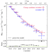 |
Fig. 11. Azimuthally averaged surface brightness profile of Abell 1795 from Chandra data with clump candidates included and excluded. The bottom panel shows the difference, where a slight decrement in the profile at the radius of the clump candidates becomes prominent when removing these sources. The best-fit power-law also becomes moderately steeper with the 24 clump candidates removed, with the best-fit α increasing from 4.18 ± 0.13 to 4.34 ± 0.09. This steepening, however, is attributed mainly to the relatively large difference between the last data points and the associated uncertainties. |
4.3. Variations in the Suzaku surface brightness profile caused by unresolved point sources
Thanks to the high spatial resolution of Chandra (with a PSF that is 100 times smaller than that of Suzaku) we resolved 1137 point sources in the 0.5 − 2 keV energy band down to fluxes of > 10−15 erg s−1 cm−1 (Sects. 2.1.2 and 3.3). In contrast, the number of sources resolved by Suzaku is 29 (Sect. 3.2.1). However, we note that the field coverage of the two telescopes is not identical (Fig. 1). Despite Suzaku’s excellence in low surface brightness studies, any mistreatment with respect to the source exclusion may distort the measurements.
To probe the impact of Suzaku’s low spatial resolution on imaging measurements, we extracted and fit a surface brightness profile based on purely Suzaku data, that is, masking only the 29 Suzaku-resolved sources, which we compared with the profile presented in Sect. 3.2.1. Within error bars, the two profiles are in agreement with only ≲8% difference measured between the best-fit power-law exponents, suggesting only a slight improvement with the inclusion of Chandra data.
4.4. Excess ICM emission towards the west
The surface brightness distribution extracted in the western direction displays a 4.2σ enhancement relative to the azimuthally averaged profile in the Chandra observations of the cluster outskirts (Sect. 3.2.2, Fig. 6). For further analysis, we subdivided the western extraction region into three equal-sized sectors with an opening angle of 30° and measured the surface brightness profile within each sector. We found that the surface brightness excess is the most prominent in the southernmost, then the central of the western sub-sectors.
To explore the cluster’s cosmic environment, we built the galaxy distribution in the large-scale surroundings and looked for structures (i.e., galaxy concentrations) that may be linked to the excess surface brightness. We searched for galaxies in SDSS DR16 within a 5° radius around Abell 1795 and within a redshift range of 0.0552 − 0.0692 (Wagner et al. 2018). With the same method described in Sect. 3.1.1, we also estimated the stellar mass of the galaxies so that a stellar mass filter can be applied when mapping the galaxy distribution. The resulting maps are displayed in Fig. 12.
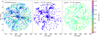 |
Fig. 12. Large-scale environment of Abell 1795. Left: spatial distribution of galaxies centered around Abell 1795. Dashed lines denote the direction of the surface brightness extraction regions, but note that the Chandra FoV is limited to the area marked by the central black circle. Black crosses indicate the location of neighboring clusters, among which Abell 1775 is one of the richest in galaxies, and towards which a surface brightness excess was observed in the outskirts of Abell 1795. Middle: filamentary structures in the distribution of high-mass galaxies. Right: low-mass galaxies, populating volume-filling sheets and voids, producing a homogeneous distribution. |
The distribution of galaxies shows filamentary structures, which are the most prominent when plotting only the relatively large-mass galaxies (log M* > 10.3 M⊙) (Fig. 12, middle panel), while the distribution of low-mass galaxies (log M* < 9.7 M⊙) is relatively homogeneous (Fig. 12, right panel). Filtering the sample based on stellar mass is reasonable because massive galaxies (log Mhalo ≳ 11.5 M⊙) almost exclusively reside within the filaments, while low-mass galaxies are typically scattered around the field, populating walls and voids, thus producing a more even distribution (Aragón-Calvo et al. 2007; Hahn et al. 2007; Cautun et al. 2014). The spatial configuration of galaxy concentrations in Fig. 12 is in agreement with the filaments found in UV absorption studies by Bregman et al. (2004). The thickness (i.e., the galaxy richness) and direction of the filaments, however, vary with the location. In addition, the scales on which the filaments are already outlined in the galaxy distribution, are not comparable to the Chandra FoV of Abell 1795. Thus, the association between the SB excess and large-scale filaments becomes more complicated.
In the left panel of Fig. 12, we also indicate the position of the neighboring galaxy clusters, which are, together with Abell 1795, members of the Boötes supercluster. The richest of the members is Abell 1795, along with Abell 1775 (Abell et al. 1989), which lies in the projected direction of the surface brightness excess present in Abell 1795. As no indication of excess towards Abell 1795 was found in the surface brightness profile of Abell 1775 extracted from XMM-Newton data out to ≳r200, we speculate that the measured surface brightness excess might be related to infall along a filament.
The surface brightness excess towards the west is also well pronounced when selecting azimuthal slices specifically based on the direction of galaxy filaments. Using this approach, we found no surface brightness excess towards other filaments.
4.5. Electron-ion non-equilibrium and non-thermal pressure support
Clumps disrupt the homogeneity of the ICM, and bias its density profile high. It leads to the classical observational signs of ICM clumping, namely an increased pressure (P ∼ ne) and, more importantly, a flattened entropy ( ) compared to the profiles with pure gravitational heating. We note that cluster observations suggest that the entropy is more sensitive to dynamical history and non-gravitational processes (Arnaud et al. 2010). In Abell 1795, however, the entropy (K ∼ kT) measurements are biased low in the outskirts, and the pressure (P ∼ kT) is consistent with the empirical model of Arnaud et al. (2010); although it is slightly steeper in the outskirts compared to the baseline of Planck Collaboration Int. V (2013; Fig. 9, R2–3 profiles), which, in turn, is indicative of a temperature bias.
The presence of a temperature bias and absence of a density bias in the outskirts of Abell 1795 are also confirmed by the self-similarly scaled profiles (Fig. 13) built following Walker et al. (2013). The reference temperature and electron number density models adopt the universal pressure profile from Planck Collaboration Int. V (2013) and the baseline entropy profile proposed by Pratt et al. (2010) to describe the ICM. The mass within an overdensity of 500 (M500 = 5.33 × 10¹⁴ M⊙) and the corresponding radius (r500 = 16.82′) of Abell 1795 were adopted from Eckert et al. (2017). Both the models and measurements are scaled by the K500 self-similar entropy (Sect. 3.4.3) and P500 self-similar pressure (Sect. 3.4.4) at r500, enabling a comparison of shape and normalization between the baseline profiles and measurements.
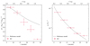 |
Fig. 13. Self-similarly scaled profiles of measured and modeled properties of Abell 1795. The reference models represent an ICM where the universal pressure profile from the Planck Collaboration Int. V (2013) and the entropy profile of Pratt et al. (2010) apply. We note that the outermost measurements are not reliable due to the large uncertainties introduced during deprojection. Left: lower-than-expected temperature in the outskirts of Abell 1795 indicates the influence of complex dynamics in the physics of the outskirts. This may support theories suggesting electron–ion non-equilibrium and non-thermal pressure support to be at play in the cluster outskirts. Right: outskirts of Abell 1795 show no excess in the electron number density, implying the successful resolution of point sources and the absence of resolved or unresolved clumping in the ICM gas. |
Low temperature values in the outskirts could be attributed to non-equilibrium effects (Hoshino et al. 2010; Akamatsu et al. 2012; Avestruz et al. 2016). When a plasma of electrons and ions travels through a shock, the heavier ions tend to absorb most of the kinetic energy and heat to Ti ≫ Te. Thus, while the system eventually reaches equilibrium, the electron temperature may be lower than the ion temperature. As CCD spectroscopy is only able to measure the electron temperature, in the presence of non-equilibrium conditions, the mean gas temperature may be underestimated. In the absence of physical processes able to couple the temperature of particles (e.g., interactions driven by magnetic fields), the equilibration timescale for a fully ionized ICM is given by (Spitzer 1962; Rudd & Nagai 2009):
where ln Λ is the Coulomb logarithm. We substituted Te and ni from the R3 measurements of the outermost annulus and obtained tei ≈ 1.7 × 10⁸yr for Abell 1795, which is much smaller than the cluster age. Therefore, if indeed present, electron–ion non-equilibrium would indicate a recent dynamical event in the outskirts.
In addition, the thermodynamic properties of the ICM might also be influenced by non-thermal pressure due to turbulent and bulk gas motions in the plasma. However, the measurements of Eckert et al. (2019) at r500 and r200 in Abell 1795 indicate non-thermal pressure ratios of only  and
and  , respectively. These fractions are below the median of the rest of the sample, which comprises clusters from the XMM-Newton cluster outskirts project (Eckert et al. 2017), and suggest that only a small fraction of the energy is attributed to kinetic motions.
4.6. Unidentified clumps among point sources
During point source detection with wavdetect, we applied a reduced signal threshold of 10−8, so that the weakest sources, including potential ICM clumps, remain undetected at this phase of the analysis (Sect. 2.1.2). Later in the analysis, no confirmed clumps were found among the list of clump candidates. In fact, these candidates turned out to be background AGN, galaxies, or galaxy clusters or groups (Appendix A, Table 4). Despite the reduced signal threshold, it should be verified that no clumps were detected in the wavdetect output source list. For this end, we picked out the most extended and least luminous sources from the list, namely, those having the same characteristics as clumps. As we found a slight positive trend between the PSF ratio ( ) and the net count rate of the sources, we only applied a limit to the PSF ratio of > 1.25, to which 35 sources correspond.
To get an impression of the type of selected sources, we built their combined spectrum. This way, we ensured that the number of source counts was sufficient for spectral extraction. The background treatment was carried out using local background annuli for each source within a radius of twice the source major axis. We found that the combined source spectrum follows a power-law model with a best-fit photon index of Γ = 1.39 ± 0.03. It suggests that the most extended sources in the wavdetect output are most likely to be AGN – and not ICM clumps. This conclusion is in agreement with Sect. 3.3, where we found no significant excess in the log N − log S distribution of the wavdetect identified sources compared to those constructed for CDFS point sources. However, we note that cosmic variance, as such, may blur the effect of ICM clumps and thereby hinder bulk clump detection using the log N − log S plot.
5. Conclusions
We present a joint analysis of high-angular-resolution Chandra ACIS-I and high-sensitivity Suzaku XIS data of the Abell 1795 cluster outskirts with the aim of isolating ICM inhomogeneities and building the radial profiles of main ICM properties out to very large radii. The imaging analysis and the projected profiles probe the cluster outskirts beyond r200, while the radial profile of deprojected thermodynamic properties extends to r200. Our findings are summarized below.
-
We identified 24 clump candidates in the projected field of Abell 1795. Based on their multi-waveband properties, the candidates can be typically associated with background objects, thus, they are not genuine ICM clumps.
-
The impact of the 24 clump candidates on the surface brightness and thermodynamic profiles of the ICM is marginal.
-
Due to the cosmic variance, the effect of clumping cannot be detected in the log N − log S plot of field sources. In fact, these sources are expected to be solely AGN.
-
The surface brightness profile extracted from Chandra observations is in agreement with that extracted from Suzaku. Excess ICM emission towards the west is seen in the direction of Abell 1775, a rich neighbor of Abell 1795.
-
Upon removal of clump candidates from the ICM, the emissivity bias profile flattens at ∼1, indicating no or only marginal unresolved clumping in Abell 1795.
-
After removing all detected Chandra sources (including both point sources and clump candidates), the entropy profile of the ICM still departs from what is expected from a purely gravitational infall. The shape of the profile indicates hints for complex physics governing the outskirts, including potential electron–ion non-equilibrium and non-thermal pressure support.
These findings shed new light on ICM clumping studies and provide a robust foundation for the development of next-generation cosmological simulations.
Acknowledgments
We thank for the anonymous referee’s useful comments. O.E.K. and N.W. are supported by the GAČR EXPRO grant No. 21-13491X “Exploring the Hot Universe and Understanding Cosmic Feedback”. This paper benefited from a visit supported by European Union’s 2020 research and innovation program under grant agreement No. 871158, project AHEAD2020. The authors thank Dan Hu for her useful contribution to the XMM-Newton analysis of Abell 1775. A.S. and Z.Z. are supported by the Women In Science Excel (WISE) programme of the Netherlands Organisation for Scientific Research (NWO). A.S. acknowledges the Kavli IPMU for the continued hospitality. Á.B. acknowledges support from the Smithsonian Institution and the Chandra X-ray Center through NASA contract NAS8-03060.
References
- Abell, G. O., Corwin, H. G., Jr, & Olowin, R. P. 1989, ApJS, 70, 1 [Google Scholar]
- Akamatsu, H., Hoshino, A., Ishisaki, Y., et al. 2011, PASJ, 63, S1019 [CrossRef] [Google Scholar]
- Akamatsu, H., de Plaa, J., Kaastra, J., et al. 2012, PASJ, 64, 49 [NASA ADS] [Google Scholar]
- Aragón-Calvo, M. A., van de Weygaert, R., Jones, B. J. T., & van der Hulst, J. M. 2007, ApJ, 655, L5 [Google Scholar]
- Arnaud, K. A. 1996, ASP Conf. Ser., 101, 17 [Google Scholar]
- Arnaud, M., Pratt, G. W., Piffaretti, R., et al. 2010, A&A, 517, A92 [CrossRef] [EDP Sciences] [Google Scholar]
- Avestruz, C., Nagai, D., & Lau, E. T. 2016, ApJ, 833, 227 [NASA ADS] [CrossRef] [Google Scholar]
- Bartalucci, I., Mazzotta, P., Bourdin, H., & Vikhlinin, A. 2014, A&A, 566, A25 [NASA ADS] [CrossRef] [EDP Sciences] [Google Scholar]
- Battaglia, N., Bond, J. R., Pfrommer, C., & Sievers, J. L. 2012, ApJ, 758, 74 [NASA ADS] [CrossRef] [Google Scholar]
- Bautz, M. W., Miller, E. D., Sanders, J. S., et al. 2009, PASJ, 61, 1117 [NASA ADS] [Google Scholar]
- Bell, E. F., McIntosh, D. H., Katz, N., & Weinberg, M. D. 2003, ApJS, 149, 289 [Google Scholar]
- Bogdán, Á., & Gilfanov, M. 2011, MNRAS, 418, 1901 [Google Scholar]
- Bregman, J. N., Dupke, R. A., & Miller, E. D. 2004, ApJ, 614, 31 [NASA ADS] [CrossRef] [Google Scholar]
- Cappelluti, N., Hasinger, G., Brusa, M., et al. 2007, ApJS, 172, 341 [NASA ADS] [CrossRef] [Google Scholar]
- Cautun, M., van de Weygaert, R., Jones, B. J. T., & Frenk, C. S. 2014, MNRAS, 441, 2923 [Google Scholar]
- de Plaa, J. 2017, https://doi.org/10.5281/zenodo.2575495 [Google Scholar]
- de Vries, M., Mantz, A. B., Allen, S. W., et al. 2023, MNRAS, 518, 2954 [Google Scholar]
- Ebeling, H., Edge, A. C., Bohringer, H., et al. 1998, MNRAS, 301, 881 [Google Scholar]
- Eckert, D., Molendi, S., & Paltani, S. 2011, A&A, 526, A79 [NASA ADS] [CrossRef] [EDP Sciences] [Google Scholar]
- Eckert, D., Vazza, F., Ettori, S., et al. 2012, A&A, 541, A57 [NASA ADS] [CrossRef] [EDP Sciences] [Google Scholar]
- Eckert, D., Molendi, S., Vazza, F., Ettori, S., & Paltani, S. 2013, A&A, 551, A22 [NASA ADS] [CrossRef] [EDP Sciences] [Google Scholar]
- Eckert, D., Roncarelli, M., Ettori, S., et al. 2015, MNRAS, 447, 2198 [Google Scholar]
- Eckert, D., Ettori, S., Pointecouteau, E., et al. 2017, Astron. Nachr., 338, 293 [Google Scholar]
- Eckert, D., Ghirardini, V., Ettori, S., et al. 2019, A&A, 621, A40 [NASA ADS] [CrossRef] [EDP Sciences] [Google Scholar]
- George, M. R., Fabian, A. C., Sanders, J. S., Young, A. J., & Russell, H. R. 2009, MNRAS, 395, 657 [Google Scholar]
- Ghirardini, V., Ettori, S., Eckert, D., et al. 2018, A&A, 614, A7 [NASA ADS] [CrossRef] [EDP Sciences] [Google Scholar]
- Giacconi, R., Rosati, P., Tozzi, P., et al. 2001, ApJ, 551, 624 [Google Scholar]
- Gilfanov, M. 2004, MNRAS, 349, 146 [NASA ADS] [CrossRef] [Google Scholar]
- Goulding, A. D., Greene, J. E., Ma, C.-P., et al. 2016, ApJ, 826, 167 [Google Scholar]
- Grimm, H. J., Gilfanov, M., & Sunyaev, R. 2003, MNRAS, 339, 793 [Google Scholar]
- Hahn, O., Porciani, C., Carollo, C. M., & Dekel, A. 2007, MNRAS, 375, 489 [NASA ADS] [CrossRef] [Google Scholar]
- Hall, D., Holland, A., & Turner, M. 2007, SPIE Conf. Ser., 6686, 66860J [NASA ADS] [Google Scholar]
- Hao, J., McKay, T. A., Koester, B. P., et al. 2010, ApJS, 191, 254 [Google Scholar]
- Hasinger, G., Altieri, B., Arnaud, M., et al. 2001, A&A, 365, L45 [NASA ADS] [CrossRef] [EDP Sciences] [Google Scholar]
- Hickox, R. C., & Markevitch, M. 2006, ApJ, 645, 95 [NASA ADS] [CrossRef] [Google Scholar]
- Hoshino, A., Henry, J. P., Sato, K., et al. 2010, PASJ, 62, 371 [CrossRef] [Google Scholar]
- Irwin, J. A., Athey, A. E., & Bregman, J. N. 2003, ApJ, 587, 356 [NASA ADS] [CrossRef] [Google Scholar]
- Jones, C., & Forman, W. 1984, ApJ, 276, 38 [NASA ADS] [CrossRef] [Google Scholar]
- Kawahara, H., Reese, E. D., Kitayama, T., Sasaki, S., & Suto, Y. 2008, ApJ, 687, 936 [NASA ADS] [CrossRef] [Google Scholar]
- Kawaharada, M., Okabe, N., Umetsu, K., et al. 2010, ApJ, 714, 423 [Google Scholar]
- Khedekar, S., Churazov, E., Kravtsov, A., et al. 2013, MNRAS, 431, 954 [Google Scholar]
- Kim, D.-W., & Fabbiano, G. 2013, ApJ, 776, 116 [NASA ADS] [CrossRef] [Google Scholar]
- Kim, D.-W., James, N., Fabbiano, G., Forbes, D., & Alabi, A. 2019, MNRAS, 488, 1072 [Google Scholar]
- Kuntz, K. D., & Snowden, S. L. 2000, ApJ, 543, 195 [Google Scholar]
- Lehmer, B. D., Xue, Y. Q., Brandt, W. N., et al. 2012, ApJ, 752, 46 [NASA ADS] [CrossRef] [Google Scholar]
- Lodders, K., Palme, H., & Gail, H. P. 2009, Landolt Börnstein, 4B, 712 [Google Scholar]
- Luo, B., Brandt, W. N., Xue, Y. Q., et al. 2017, ApJS, 228, 2 [Google Scholar]
- Markevitch, M., Ponman, T. J., Nulsen, P. E. J., et al. 2000, ApJ, 541, 542 [Google Scholar]
- Markevitch, M., Bautz, M. W., Biller, B., et al. 2003, ApJ, 583, 70 [Google Scholar]
- Mathiesen, B., Evrard, A. E., & Mohr, J. J. 1999, ApJ, 520, L21 [NASA ADS] [CrossRef] [Google Scholar]
- McConnachie, A. W., Patton, D. R., Ellison, S. L., & Simard, L. 2009, MNRAS, 395, 255 [NASA ADS] [CrossRef] [Google Scholar]
- Mernier, F., de Plaa, J., Lovisari, L., et al. 2015, A&A, 575, A37 [NASA ADS] [CrossRef] [EDP Sciences] [Google Scholar]
- Mohr, J. J., Mathiesen, B., & Evrard, A. E. 1999, ApJ, 517, 627 [Google Scholar]
- Morandi, A., & Cui, W. 2014, MNRAS, 437, 1909 [Google Scholar]
- Moretti, A., Campana, S., Lazzati, D., & Tagliaferri, G. 2003, ApJ, 588, 696 [NASA ADS] [CrossRef] [Google Scholar]
- Nagai, D., & Lau, E. T. 2011, ApJ, 731, L10 [NASA ADS] [CrossRef] [Google Scholar]
- Nagai, D., Kravtsov, A. V., & Vikhlinin, A. 2007, ApJ, 668, 1 [Google Scholar]
- Park, T., Kashyap, V. L., Siemiginowska, A., et al. 2006, ApJ, 652, 610 [Google Scholar]
- Piconcelli, E., Jimenez-Bailón, E., Guainazzi, M., et al. 2005, A&A, 432, 15 [NASA ADS] [CrossRef] [EDP Sciences] [Google Scholar]
- Planck Collaboration Int. V. 2013, A&A, 550, A131 [NASA ADS] [CrossRef] [EDP Sciences] [Google Scholar]
- Pratt, G. W., Arnaud, M., Piffaretti, R., et al. 2010, A&A, 511, A85 [NASA ADS] [CrossRef] [EDP Sciences] [Google Scholar]
- Rasia, E., Lau, E. T., Borgani, S., et al. 2014, ApJ, 791, 96 [NASA ADS] [CrossRef] [Google Scholar]
- Reeves, J. N., & Turner, M. J. L. 2000, MNRAS, 316, 234 [NASA ADS] [CrossRef] [Google Scholar]
- Reiprich, T. H., Hudson, D. S., Zhang, Y. Y., et al. 2009, A&A, 501, 899 [NASA ADS] [CrossRef] [EDP Sciences] [Google Scholar]
- Richards, G. T., Myers, A. D., Gray, A. G., et al. 2009, ApJS, 180, 67 [Google Scholar]
- Roncarelli, M., Ettori, S., Borgani, S., et al. 2013, MNRAS, 432, 3030 [NASA ADS] [CrossRef] [Google Scholar]
- Rozo, E., Rykoff, E. S., Becker, M., Reddick, R. M., & Wechsler, R. H. 2015, MNRAS, 453, 38 [NASA ADS] [CrossRef] [Google Scholar]
- Rudd, D. H., & Nagai, D. 2009, ApJ, 701, L16 [NASA ADS] [CrossRef] [Google Scholar]
- Sabol, E. J., & Snowden, S. L. 2019, Astrophysics Source Code Library [record ascl:1904.001] [Google Scholar]
- Sanders, J. S. 2006, MNRAS, 371, 829 [Google Scholar]
- Sato, T., Sasaki, T., Matsushita, K., et al. 2012, PASJ, 64, 95 [NASA ADS] [CrossRef] [Google Scholar]
- Simionescu, A., Allen, S. W., Mantz, A., et al. 2011, Science, 331, 1576 [Google Scholar]
- Simionescu, A., Werner, N., Urban, O., et al. 2013, ApJ, 775, 4 [Google Scholar]
- Snowden, S. L., Freyberg, M. J., Plucinsky, P. P., et al. 1995, ApJ, 454, 643 [Google Scholar]
- Snowden, S. L., Mushotzky, R. F., Kuntz, K. D., & Davis, D. S. 2008, A&A, 478, 615 [NASA ADS] [CrossRef] [EDP Sciences] [Google Scholar]
- Spitzer, L. 1962, Physics of Fully Ionized Gases (Hoboken, NJ: John Wiley and Sond, Inc.) [Google Scholar]
- Strateva, I., Ivezić, Ž., Knapp, G. R., et al. 2001, AJ, 122, 1861 [CrossRef] [Google Scholar]
- Tawa, N., Hayashida, K., Nagai, M., et al. 2008, PASJ, 60, S11 [NASA ADS] [Google Scholar]
- Urban, O., Werner, N., Simionescu, A., Allen, S. W., & Böhringer, H. 2011, MNRAS, 414, 2101 [NASA ADS] [CrossRef] [Google Scholar]
- Urban, O., Simionescu, A., Werner, N., et al. 2014, MNRAS, 437, 3939 [Google Scholar]
- Urban, O., Werner, N., Allen, S. W., Simionescu, A., & Mantz, A. 2017, MNRAS, 470, 4583 [Google Scholar]
- Vazza, F., Eckert, D., Simionescu, A., Brüggen, M., & Ettori, S. 2013, MNRAS, 429, 799 [Google Scholar]
- Vikhlinin, A., Markevitch, M., Murray, S. S., et al. 2005, ApJ, 628, 655 [Google Scholar]
- Vikhlinin, A., Kravtsov, A., Forman, W., et al. 2006, ApJ, 640, 691 [Google Scholar]
- Voit, G. M., Kay, S. T., & Bryan, G. L. 2005, MNRAS, 364, 909 [NASA ADS] [CrossRef] [Google Scholar]
- Wagner, C. R., McDonald, M., & Courteau, S. 2018, ApJ, 867, 14 [NASA ADS] [CrossRef] [Google Scholar]
- Walker, S. A., Fabian, A. C., Sanders, J. S., & George, M. R. 2012, MNRAS, 427, L45 [Google Scholar]
- Walker, S. A., Fabian, A. C., Sanders, J. S., Simionescu, A., & Tawara, Y. 2013, MNRAS, 432, 554 [Google Scholar]
- Wen, Z. L., & Han, J. L. 2015, ApJ, 807, 178 [Google Scholar]
- Werner, N., Urban, O., Simionescu, A., & Allen, S. W. 2013, Nature, 502, 656 [Google Scholar]
- Willingale, R., Starling, R. L. C., Beardmore, A. P., Tanvir, N. R., & O’Brien, P. T. 2013, MNRAS, 431, 394 [Google Scholar]
- Yoshino, T., Mitsuda, K., Yamasaki, N. Y., et al. 2009, PASJ, 61, 805 [NASA ADS] [Google Scholar]
- Zhu, Z., Simionescu, A., Akamatsu, H., et al. 2021a, A&A, 652, A147 [NASA ADS] [CrossRef] [EDP Sciences] [Google Scholar]
- Zhu, Z., Xu, H., Hu, D., et al. 2021b, ApJ, 908, 17 [NASA ADS] [CrossRef] [Google Scholar]
- Zhu, Z., Kovács, O. E., Simionescu, A., & Werner, N. 2023, A&A, in press, https://doi.org/10.1051/0004-6361/202347191 [Google Scholar]
- Zhuravleva, I., Churazov, E., Kravtsov, A., et al. 2013, MNRAS, 428, 3274 [NASA ADS] [CrossRef] [Google Scholar]
- Zou, H., Gao, J., Xu, X., et al. 2021, ApJS, 253, 56 [NASA ADS] [CrossRef] [Google Scholar]
Appendix A: Origins of individual clump candidates
We based the classification of clump candidates on the results from Sections 3.1.1 and 3.1.2. Their descriptions are given below.
C1 is located near the chip edge and therefore has a large PSF, which complicates source characterization. The positive hardness ratio, however, is not indicative of diffuse thermal emission expected from gas clumps.
C2 does not exhibit a definite X-ray peak, although the local PSF is relatively large. It overlaps with three background galaxies. However, based on the estimated X-ray flux of these galaxies, they do not account for the detected X-ray emission. The positive hardness ratio suggests a possible AGN origin.
C3 exhibits a well-defined excess emission that peaks around a previously detected and removed wavdetect source and coincides with 4 SDSS-galaxies at relatively high redshifts (z = 0.41 − 0.59). As the estimated X-ray flux from the overlapping galaxies cannot explain the measured flux, it is likely that the main contributors are the AGN in these background galaxies, smeared out in the X-ray image.
C4 is associated with a previously detected X-ray source’s extended emission. This X-ray source coincides with 3 background galaxies, of which none is expected to display a detectable amount of X-ray emission. With an offset of 0.012′, the NASA/IPAC Extragalactic Database (NED) lists a galaxy cluster (X-CLASS 1684) with an unknown redshift. In addition, with a larger offset of ∼0.12′, a rich galaxy cluster identified in the DESI Legacy Imaging Surveys (Zou et al. 2021) lies at z ≈ 0.80, encompassing the source of interest. We speculate that the background clusters, the X-ray source, and the clump candidate are the same source. The temperature kT = 3.3 ± 0.6 keV from the spectral fit of the X-ray source is consistent with this explanation.
C5 exhibits a peak emission that encloses two previously excluded wavdetect sources, one of them exhibiting extended emission, which was missed by wavdetect, and it was later identified as a clump candidate. For this wavdetect source, an Abell 1795 member galaxy counterpart was found in the SDSS data at zspec = 0.061 with a stellar mass of M∗ ≈ 3 × 10¹¹ M⊙. The expected X-ray flux of the galaxy, F0.7−2 keV ≈ 1.0 × 10⁻¹⁴ erg cm−2 s−1, is comparable with the flux measured for the clump candidate (F0.7−2 keV ≈ 1.2 × 10⁻¹⁴ erg cm−2 s−1). The galaxy’s spectrum, extracted from Chandra data, can be primarily described with an apec emission with kT = (0.82 ± 0.10) keV, which, along with the hardness ratio, indicates that the galaxy’s diffuse emission is what was misidentified as a clump.
C6 coincides with an SDSS galaxy at z ≈ 0.18 with an estimated stellar mass of M∗ ≈ 3.6 × 10¹¹ M⊙ and an estimated X-ray emission (F0.7−2 keV ≈ 1.8 × 10⁻¹⁵ erg cm−2 s−1) comparable to C6’s measured flux (F0.7−2 keV ≈ 2.6 × 10⁻¹⁵ erg cm−2 s−1). The match between C6 and the co-spatial galaxy is also reflected in the candidate’s HR ≈ 0.5 hardness ratio.
C7, with a total flux of F0.7−2 keV ≈ 7.7 × 10⁻¹⁵ erg cm−2 s−1, might be physically connected with a z ≈ 0.19 background galaxy, which is the most massive one in the sample with M∗ ≈ 4.5 × 10¹¹ M⊙ and F0.7−2 keV ≈ 3.0 × 10⁻¹⁵ erg cm−2 s−1. In addition, centered at a ∼0.3′ offset to the east from this galaxy, a galaxy group (SDSSCGB 11608) is located at z = 0.173 (McConnachie et al. 2009) within the C7 region.
C8 shows two X-ray peaks, one overlapping with a low-mass SDSS galaxy that is expected to display no significant X-ray emission and another point-like optical source not listed among the SDSS galaxies, but registered in NED as a red galaxy (WISEA J134810.31+260947.3). As the X-ray peaks are positioned at these objects and the estimated hardness ratio, although exhibiting large error bars, is close to zero, we suspect a physical connection between the clump and the AGN within these galaxies.
C9 has a peak that cannot be associated with an SDSS galaxy. However, an infrared object classified as an irregular source has been detected by WISE (WISEA J134655.49+262236.9) at the peak’s position, indicating a distant or low-luminosity AGN identified as clump candidate.
C10 shows diffuse emission extending outside the candidate’s region, where a massive (M∗ ≈ 3.7 × 10¹¹ M⊙), but relatively distant (z ≈ 0.55) SDSS galaxy is located. Its expected X-ray emission is approximately an order of magnitude lower than that measured within the C10 region. The extension of the diffuse X-ray emission within C10, similarly to C9, can be associated with an irregular source identified with WISE (WISEA J134844.78+270520.8).
C11 is characterized by a positive hardness ratio that does not indicate diffuse gas emission. However, no objects in SDSS have been reported at the position of the X-ray excess, nor at the position of the closest wavdetect source, thus making a possible AGN origin also questionable.
C12 can be associated with a background galaxy cluster, WHL J134645.8+264625 at z = 0.4271 (Wen & Han 2015) located at and extending beyond the southern region of C12, where an X-ray excess is indeed prominent.
C13 is visibly linked with a background AGN (WISEA J134636.14+262715.7) located at z = 0.305 (Richards et al. 2009). This connection is supported by the positive hardness ratio measured within the candidate’s region.
C14 exhibits a peak emission that coincides with a low-mass background galaxy. However, it is not sufficient to explain the detected X-ray excess. The overall positive hardness ratio might suggest the presence of an AGN hosted by this galaxy but note that the northern part of the clump candidate, including the peak, possibly overlaps with the outskirts of a z ≈ 0.74 galaxy cluster identified in DESI.
C15’s classification is identical to that of C13, with the candidate’s emission described as excess power-law radiation (note the close to zero hardness ratio) from a background AGN (WISEA J135022.71+261003.8) at z = 1.343806.
C16 is associated with two background galaxies. The closest (zspec = 0.178) is the more massive one with M∗ ≈ 2.7 × 10¹¹ M⊙, and with an estimated X-ray flux of F0.7−2 keV ≈ 8.9 × 10⁻¹⁶ erg cm−2 s−1, a factor of ∼ 6.6 fainter compared to the total flux measured within C16. Comparison with a smaller region at the galaxy’s position within C16, however, yields a good agreement between the measured and the expected X-ray fluxes. North of the massive galaxy lies a possible AGN detected as an irregular IR source by WISE (WISEA J134817.26+260338.8). Although the negative hardness ratio measured throughout C16 indicates diffuse emission, the relatively large PSF, along with the small projected distance between these objects, complicates the source classification.
C17 overlaps with a background galaxy cluster (WHL J 134950.2 + 270623) lying at z ≈ 0.42 (Rozo et al. 2015) and the X-ray emission detected as a clump candidate may originate from its ICM. This is confirmed by the negative hardness ratio and its small error bars.
C18 is arranged around a wavdetect source, registered in SDSS as a background galaxy (z ≈ 0.6), and encompasses two low-mass background galaxies (z ≈ 0.4). Based on the analysis of SDSS data, none of these can explain the measured X-ray flux. However, the co-spatial alignment of the X-ray and optical sources, as well as the hardness ratio, point towards an AGN origin for C18’s emission.
C19 displays a weak excess that consists of two equally bright peaks, of which one is co-aligned with two SDSS galaxies, one lying in the background and the other one possibly gravitationally bound to A1795 with a photometric redshift of ∼0.095 ± 0.027. The second X-ray peak has no optical counterpart. Although C19 is a weak source and its hardness ratio is inconclusive, we cannot rule out that it includes a genuine clump.
C20 may be physically connected with a background quasar (WISEA J 134643.44 + 265417.6) lying at z ≈ 1.75 (Richards et al. 2009). The estimated hardness ratio of HR ≈ 0.1 also supports this connection.
C21 overlaps with two low-mass SDSS galaxies in the background (z ≈ 0.4 − 0.5), none of which is expected to account for the measured X-ray flux. The galaxy to which C21 is attached and was detected by wavdetect shares similar properties, but it is cataloged in WISE as an irregular source; thus, it is likely to be an AGN. Although the large error bars on the hardness ratio and the large local PSF in this field complicate source characterization, it cannot be ruled out that C21’s emission may be associated with a background AGN.
C22’s observed emission remains elusive. The single SDSS galaxy coinciding with the candidate is a low-mass background system. Within 0.1′ of the X-ray peak, three objects are registered in NED: two point sources and an ultraviolet source. In addition, within ∼0.65′ to the northeastern direction lies a distant galaxy cluster (GMBCG J206.84924+27.13581) at z = 0.402 (Hao et al. 2010) (note: the smallest fitting circle of C22 is ∼0.45′).
C23 and C24, located at the chip edge, are smeared by the large local PSF. Thus, they cannot be classified.
Appendix B: Uncertainties in the projected temperature profile introduced by systematic effects
According to the estimated 25% fluctuation in the level of the galactic halo (GH) emission (Section 2.2.4), the R1 and R3 spectral fits were repeated with the normalization of the corresponding apec model fixed at the ±25% values of the best-fit normalization. The kT measurements obtained this way represent the upper and lower boundaries of the systematic error from GH fluctuations and are plotted with hatched regions in FigureB.1. The uncertainties in kT introduced by the relative cosmic variance (Section 2.2.4) were computed similarly, and the resulting kT intervals are illustrated in FigureB.1 as the shaded regions. These results show that the systematic errors are below the statistical ones and the present Suzaku measurements are not dominated by systematic uncertainties.
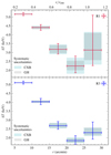 |
Fig. B.1. Demonstration of systematic effects on the projected R1 and R3 kT profiles caused by spatial variations in the cosmic X-ray background and in the galactic halo emission. |
All Tables
Surface brightness distribution parameters from the adaptively binned image in five annuli.
All Figures
|
Fig. 1. FoV comparison between the exposure and background corrected 0.7 − 2 keV Chandra ACIS-I mosaic (left panel) and the exposure and vignetting corrected 0.7 − 7 keV Suzaku XIS mosaic (right panel) of Abell 1795. Images are to scale, but the smoothness and the color scales are not identical due to the different image sensitivities. The location of r500 and r200 is marked with the inner and outer circles, respectively, and on the right panel we also marked the Suzaku resolved point source regions with white. |
| In the text | |
|
Fig. 2. Adaptively binned image of Abell 1795 outskirts in the 0.7 − 2 keV energy band. The image is instrumental background- and exposure-corrected. Each bin has a S/N of ≳3, and a surface brightness value indicated by the colorbar in photon cm−2 s−1 pixel−1 units. Small white ellipses scattered throughout the field represent excluded point sources. We used this image to measure the surface brightness distribution within each annulus (dashed-line circles) and to isolate outliers that may originate from ICM inhomogeneities. Outlier positions are shown with small circles marked from C1 to C24 (for the actual size and shape of the outliers, see Fig. 4). |
| In the text | |
|
Fig. 3. 0.7 − 2 keV surface brightness distribution of the ICM in the outskirts of Abell 1795 obtained in 5 annuli. The annuli extend out to ∼42.5′ as listed in Table 3. Overall, the median surface brightness coincides with the peak of the distribution, but the mean, especially at larger radii, is shifted towards high values, which suggests the presence of unresolved gas inhomogeneities (Zhuravleva et al. 2013). We selected the > + 2σ outliers of the log-normal fit within each annulus, which resulted in a total of 24 sources to form our list of clump candidates. |
| In the text | |
|
Fig. 4. Chandra 0.7 − 2 keV (left panel, color images) and SDSS r-band cutout images (right panel, greyscale images) showing the individual clump candidates (white, irregular-shaped regions) and their environment within a 200″ × 200″ area. The Chandra images are smoothed with a Gaussian of a radius of 6 to accentuate the X-ray excess. Filled black ellipses represent excluded wavdetect sources, while the filled red circle at the bottom left of each Chandra image marks the local minimum size of PSF. As most of the clump candidates overlap with multiple SDSS galaxies (green circles), possible physical connections must be addressed to isolate genuine clumps (Sects. 3.1.1 and Appendix A). |
| In the text | |
|
Fig. 4. continued. |
| In the text | |
|
Fig. 4. continued. |
| In the text | |
|
Fig. 5. 0.7 − 2 keV background-subtracted azimuthally averaged surface brightness profiles of Abell 1795 outskirts measured with Chandra and Suzaku with the corresponding best-fit power-law models overplotted. The background components are also shown. Point sources were removed down to a photon flux of 2 × 10⁻⁶ photons cm−2 s−1 from both datasets and the elevated Suzaku sky background level reflects the excess emission from point sources whose PSF is broader than the corresponding source region. |
| In the text | |
|
Fig. 6. 0.7 − 2 keV surface brightness profile of Abell 1795 outskirts extracted from Chandra data in four different directions. Azimuthal variations relative to the average profile are displayed in the bottom panel. |
| In the text | |
|
Fig. 7. Log N − log S plot for the sources detected in the Abell 1795 field (shaded curve with 1σ uncertainty) and in the 7 Ms Chandra Deep Field South (Luo et al. 2017). Despite the excess in the number of Abell 1795 field sources seen at ∼10−14 erg cm−2 s−1, which can be attributed to the cosmic variance, the distributions are in good agreement at fluxes below ∼6 × 10⁻¹⁴ erg cm−2 s−1. No excess can be explicitly attributed to unidentified clumps among wavdetect sources. |
| In the text | |
|
Fig. 8. Projected temperature profiles of the Abell 1795 cluster outskirts from three rounds (R1−3) of spectral extraction. In the R1 data, only the Suzaku resolved point sources, while from the R2 data, all point sources down to a flux of 5.8 × 10⁻¹⁵ erg cm−2 s−1 were removed. The R3 profile, on top of that, accounts for the effect of the resolved clump candidates, which is insignificant. For comparison, we included three additional profiles from previous works. |
| In the text | |
|
Fig. 9. Deprojected profiles of the cluster outskirts with R1−3 denoting the deprojected equivalents of the profiles shown in Fig. 8 (Sect. 2.2.2). The outermost data points, shown with dashed lines, exhibit large uncertainties introduced with the deprojection. Top left: comparison between the deprojected and the projected temperature profiles. Top right: electron density profiles overplotted with ROSAT measurements of the same cluster by Eckert et al. (2013). Bottom left: entropy profiles compared with the profile of Pratt et al. (2010), which models a galaxy cluster formed by gravitational collapse with no additional heating or cooling and with the analytic function of Walker et al. (2012) fitted on a sample of Suzaku observed clusters. Bottom right: pressure profile overplotted with the best-fit models of Arnaud et al. (2010) and the Planck Collaboration Int. V (2013). |
| In the text | |
|
Fig. 10. Radial variation of the bX emissivity bias when each clump candidate is included or excluded, compared to the results from the ROSAT sample of 31 galaxy clusters (Eckert et al. 2015). The 24 clump candidates, although being not genuine clumps, cause an increased level of bias above ∼0.8 r200 in Abell 1795. When each clump candidate is excluded, the profile flattens at bX ≥ 1. Note: bX is subject to projection effects and influenced by the sky background contribution, which exhibit very different levels for the Chandra and ROSAT data sets. |
| In the text | |
|
Fig. 11. Azimuthally averaged surface brightness profile of Abell 1795 from Chandra data with clump candidates included and excluded. The bottom panel shows the difference, where a slight decrement in the profile at the radius of the clump candidates becomes prominent when removing these sources. The best-fit power-law also becomes moderately steeper with the 24 clump candidates removed, with the best-fit α increasing from 4.18 ± 0.13 to 4.34 ± 0.09. This steepening, however, is attributed mainly to the relatively large difference between the last data points and the associated uncertainties. |
| In the text | |
|
Fig. 12. Large-scale environment of Abell 1795. Left: spatial distribution of galaxies centered around Abell 1795. Dashed lines denote the direction of the surface brightness extraction regions, but note that the Chandra FoV is limited to the area marked by the central black circle. Black crosses indicate the location of neighboring clusters, among which Abell 1775 is one of the richest in galaxies, and towards which a surface brightness excess was observed in the outskirts of Abell 1795. Middle: filamentary structures in the distribution of high-mass galaxies. Right: low-mass galaxies, populating volume-filling sheets and voids, producing a homogeneous distribution. |
| In the text | |
|
Fig. 13. Self-similarly scaled profiles of measured and modeled properties of Abell 1795. The reference models represent an ICM where the universal pressure profile from the Planck Collaboration Int. V (2013) and the entropy profile of Pratt et al. (2010) apply. We note that the outermost measurements are not reliable due to the large uncertainties introduced during deprojection. Left: lower-than-expected temperature in the outskirts of Abell 1795 indicates the influence of complex dynamics in the physics of the outskirts. This may support theories suggesting electron–ion non-equilibrium and non-thermal pressure support to be at play in the cluster outskirts. Right: outskirts of Abell 1795 show no excess in the electron number density, implying the successful resolution of point sources and the absence of resolved or unresolved clumping in the ICM gas. |
| In the text | |
|
Fig. B.1. Demonstration of systematic effects on the projected R1 and R3 kT profiles caused by spatial variations in the cosmic X-ray background and in the galactic halo emission. |
| In the text | |
Current usage metrics show cumulative count of Article Views (full-text article views including HTML views, PDF and ePub downloads, according to the available data) and Abstracts Views on Vision4Press platform.
Data correspond to usage on the plateform after 2015. The current usage metrics is available 48-96 hours after online publication and is updated daily on week days.
Initial download of the metrics may take a while.