| Issue |
A&A
Volume 690, October 2024
|
|
|---|---|---|
| Article Number | A73 | |
| Number of page(s) | 18 | |
| Section | Stellar structure and evolution | |
| DOI | https://doi.org/10.1051/0004-6361/202346180 | |
| Published online | 01 October 2024 | |
HR 10 as seen by CHEOPS and TESS
Revealing δ Scuti pulsations, granulation-like signal and hint for transients⋆
1
Observatoire Astronomique de l’Université de Genève, Chemin Pegasi 51, 1290 Versoix, Switzerland
2
Space Sciences, Technologies and Astrophysics Research (STAR) Institute, Université de Liège, Allée du 6 Août 19C, 4000 Liège, Belgium
3
Aix Marseille Univ, CNRS, CNES, LAM, 38 rue Frédéric Joliot-Curie, 13388 Marseille, France
4
ELTE Eötvös Loránd University, Gothard Astrophysical Observatory, Szent Imre h. u. 112, 9700 Szombathely, Hungary
5
MTA-ELTE Exoplanet Research Group, Szent Imre h. u. 112, 9700 Szombathely, Hungary
6
Department of Astronomy, Stockholm University, AlbaNova University Center, 10691 Stockholm, Sweden
7
Physikalisches Institut, University of Bern, Sidlerstrasse 5, 3012 Bern, Switzerland
8
Center for Space and Habitability, Gesellsschaftstrasse 6, 3012 Bern, Switzerland
9
Centre Vie dans l’Univers, Faculté des sciences, Université de Genève, Quai Ernest-Ansermet 30, 1211 Genève 4, Switzerland
10
Instituto de Astrofisica e Ciencias do Espaco, Universidade do Porto, CAUP, Rua das Estrelas, 4150-762 Porto, Portugal
11
Sorbonne Université, CNRS, UMR 7095, Institut d’Astrophysique de Paris, 98 bis bd Arago, 75014 Paris, France
12
LESIA, Observatoire de Paris, Université PSL, CNRS, Sorbonne Université, Université Paris Cité, 5 place Jules Janssen, 92195 Meudon, France
13
Dipartimento di Fisica, Universita degli Studi di Torino, Via Pietro Giuria 1, 10125 Torino, Italy
14
IRAP, Université de Toulouse, CNRS, UPS, CNES, 14 Avenue Édouard Belin, 31400 Toulouse, France
15
Space Research Institute, Austrian Academy of Sciences, Schmiedlstrasse 6, 8042 Graz, Austria
16
Centre for Exoplanet Science, SUPA School of Physics and Astronomy, University of St Andrews, North Haugh, St Andrews KY16 9SS, UK
17
Instituto de Astrofisica de Canarias, 38200 La Laguna, Tenerife, Spain
18
Departamento de Astrofisica, Universidad de La Laguna, 38206 La Laguna, Tenerife, Spain
19
Institut de Ciencies de l’Espai (ICE, CSIC), Campus UAB, Can Magrans s/n, 08193 Bellaterra, Spain
20
Institut d’Estudis Espacials de Catalunya (IEEC), 08034 Barcelona, Spain
21
Admatis, 5. Kandó Kálmán Street, 3534 Miskolc, Hungary
22
Depto. de Astrofisica, Centro de Astrobiologia (CSIC-INTA), ESAC campus, 28692 Villanueva de la Cañada, Madrid, Spain
23
Departamento de Fisica e Astronomia, Faculdade de Ciencias, Universidade do Porto, Rua do Campo Alegre, 4169-007 Porto, Portugal
24
Center for Space and Habitability, University of Bern, Gesellschaftsstrasse 6, 3012 Bern, Switzerland
25
INAF, Osservatorio Astronomico di Padova, Vicolo dell’Osservatorio 5, 35122 Padova, Italy
26
Université Grenoble Alpes, CNRS, IPAG, 38000 Grenoble, France
27
Institute of Optical Sensor Systems, German Aerospace Center (DLR), Rutherfordstrasse 2, 12489 Berlin, Germany
28
Institute of Planetary Research, German Aerospace Center (DLR), Rutherfordstrasse 2, 12489 Berlin, Germany
29
Université de Paris, Institut de physique du globe de Paris, CNRS, 75005 Paris, France
30
ESTEC, European Space Agency, 2201 AZ Noordwijk, The Netherlands
31
INAF, Osservatorio Astrofisico di Torino, Via Osservatorio, 20, 10025 Pino Torinese, To, Italy
32
Centre for Mathematical Sciences, Lund University, Box 118 221 00 Lund, Sweden
33
Astrobiology Research Unit, Université de Liège, Allée du 6 Août 19C, 4000 Liège, Belgium
34
Leiden Observatory, University of Leiden, PO Box 9513 2300 RA, Leiden, The Netherlands
35
Department of Space, Earth and Environment, Chalmers University of Technology, Onsala Space Observatory, 439 92 Onsala, Sweden
36
University of Vienna, Department of Astrophysics, Türkenschanzstrasse 17, 1180 Vienna, Austria
37
Space Research Institute, Austrian Academy of Sciences, Schmiedlstrasse 6, 8042 Graz, Austria
38
Science and Operations Department – Science Division (SCI-SC), Directorate of Science, European Space Agency (ESA), European Space Research and Technology Centre (ESTEC), Keplerlaan 1, 2201 AZ Noordwijk, The Netherlands
39
Konkoly Observatory, Research Centre for Astronomy and Earth Sciences, Konkoly Thege Miklós út 15-17, 1121 Budapest, Hungary
40
ELTE Eötvös Loránd University, Institute of Physics, Pázmány Péter sétány 1/A, 1117 Budapest, Hungary
41
IMCCE, UMR8028 CNRS, Observatoire de Paris, PSL Univ., Sorbonne Univ., 77 av. Denfert-Rochereau, 75014 Paris, France
42
Institut d’astrophysique de Paris, UMR7095 CNRS, Université Pierre & Marie Curie, 98bis blvd. Arago, 75014 Paris, France
43
Astrophysics Group, Keele University, Staffordshire ST5 5BG, UK
44
Physikalisches Institut, University of Bern, Gesellschaftsstrasse 6, 3012 Bern, Switzerland
45
Department of Astrophysics, University of Vienna, Tuerkenschanzstrasse 17, 1180 Vienna, Austria
46
INAF, Osservatorio Astrofisico di Catania, Via S. Sofia 78, 95123 Catania, Italy
47
Dipartimento di Fisica e Astronomia “Galileo Galilei”, Universita degli Studi di Padova, Vicolo dell’Osservatorio 3, 35122 Padova, Italy
48
Department of Physics, University of Warwick, Gibbet Hill Road, Coventry CV4 7AL, UK
49
ETH Zurich, Department of Physics, Wolfgang-Pauli-Strasse 2, 8093 Zurich, Switzerland
50
Cavendish Laboratory, JJ Thomson Avenue, Cambridge CB3 0HE, UK
51
Zentrum für Astronomie und Astrophysik, Technische Universität Berlin, Hardenbergstr. 36, 10623 Berlin, Germany
52
Institut für Geologische Wissenschaften, Freie Universität Berlin, 12249 Berlin, Germany
53
German Aerospace Center (DLR), Institute of Optical Sensor Systems, Rutherfordstraße 2, 12489 Berlin, Germany
54
Institute of Astronomy, University of Cambridge, Madingley Road, Cambridge CB3 0HA, UK
Received:
17
February
2023
Accepted:
15
May
2024
Context. HR 10 has only recently been identified as a binary system. Previously thought to be an A-type shell star, it appears that both components are fast-rotating A-type stars, each presenting a circumstellar envelope. Although showing complex photometric variability, spectroscopic observations of the metallic absorption lines reveal variation explained by the binarity, but not indicative of debris-disc inhomogeneities or sublimating exocomets. On the other hand, the properties of the two stars make them potential δ Scuti pulsators.
Aims. The system has been observed in two sectors by the TESS satellite, and was the target of three observing visits by CHEOPS. Thanks to these new data, we aim to further characterise the stellar properties of the two components. In particular, we aim to decipher the extent to which the photometric variability can be attributed to a stellar origin. In complement, we searched in the lightcurves for transient-type events that could reveal debris discs or exocomets.
Methods. We analysed the photometric variability of both the TESS and CHEOPS datasets in detail. We first performed a frequency analysis to identify and list all the periodic signals that may be related to stellar oscillations or surface variability. The signals identified as resulting from the stellar variability were then removed from the lightcurves in order to search for transient events in the residuals.
Results. We report the detection of δ Scuti pulsations in both the TESS and CHEOPS data, but we cannot definitively identify which of the components is the pulsating star. In both datasets, we find flicker noise with the characteristics of a stellar granulation signal. However, it remains difficult to firmly attribute it to actual stellar granulation from convection, given the very thin surface convective zones predicted for both stars. Finally, we report probable detection of transient events in the CHEOPS data, without clear evidence of their origin.
Key words: techniques: photometric / Sun: granulation / circumstellar matter / stars: fundamental parameters / stars: variables: δ Scuti
© The Authors 2024
 Open Access article, published by EDP Sciences, under the terms of the Creative Commons Attribution License (https://creativecommons.org/licenses/by/4.0), which permits unrestricted use, distribution, and reproduction in any medium, provided the original work is properly cited.
This article is published in open access under the Subscribe to Open model. Subscribe to A&A to support open access publication.
1. Introduction
Narrow absorption lines of refractory elements transiently superimposed on a stellar atmospheric spectrum are usually attributed to metal-rich material clouds surrounding the star, and generated by giant comets or icy planetesimals, which orbit this star and show strong activity or undergo a complete and fast evaporation (e.g. Beust et al. 1990; Kiefer et al. 2014; Zieba et al. 2019). Narrow-line features in shell stars have also been identified (e.g. Abt & Moyd 1973), and are thought to be a marker of the condensation processes in the matter ejected by the star. These two sources of narrow-line absorption sometimes appear side by side, as observed in the well-known case of β Pictoris (Hobbs et al. 1985). The photometric transients seen in this latter case were attributed to exocomets (Zieba et al. 2019), while a significant part of the narrow-line absorption in the stellar spectra was identified as originating from the circumstellar (hereafter CS) disc (Kiefer et al. 2014). This example demonstrates that the accurate photometric follow-up of stars with known transient narrow-line absorption components is important for two reasons: first, a possible detection of photometric components can confirm infalling or evaporating icy bodies as the main source of the narrow-line absorption, and second the non-detection of such photometric features can reveal how the stellar shell can mimic exocomets in spectral observations.
In this context, HR 10 (also known as HD 256) is an enigmatic system. Long-since identified as a shell star (Jaschek & Egret 1982), the detection of CS disc signatures later on by Lagrange-Henri et al. (1990) made HR 10 a target of interest as a candidate β Pic-like star. Nevertheless, the true nature of the HR 10 system was only recently identified by Montesinos et al. (2019, hereafter M19) as a binary thanks to interferometric observations.
The narrow absorption in K lines of Ca II is a well-known indicator of the presence of CS material; variability in these lines as well as in other metallic absorption lines is typical of the β Pic star (e.g. Hobbs et al. 1985), and other A-type stars (e.g. Roberge & Weinberger 2008). This variability is associated with gas ejection from comets grazing or falling into the star in such systems (Kiefer et al. 2014; Eiroa et al. 2016), as they are affected by the gravitational perturbation by a larger body in orbit (see models by Beust et al. 1990, 1991). Yet, in the case of Φ Leo, which is a system presenting similar spectroscopic characteristics to β Pic-like stars, Eiroa et al. (2021) questions this interpretation and highlights the potential of stellar pulsations, such as those seen for δ Scuti, to contribute to line-profile variations and to lead to misinterpretation. In this context, thanks to spectra taken over decades and in some cases covering nearly half an orbital period, M19 firmly identified, narrow absorption in Ca II K in each stellar component of HR 10, based on radial velocity (RV) decomposition. This analysis not only found that each star presents a CS envelope but rejected the presence of a circumbinary envelope. However, in combination with the spectroscopic follow-up of other metallic lines, these authors did not find evidence of other variability that could be associated with transient cometary events. The authors also noted a puzzling unsolved feature of the spectral lines in HR 10; they found that narrow-line components are always redshifted in regards to CS lines likely associated with each star, with a surprisingly stable offset in the order of 8–11 km/s. The stable redshift of the narrow lines suggests matter moving towards the star with significant velocity (see also Welsh & Montgomery 2018), which is not compatible with a stable structure around the star. This observation suggests the possibility of infalling matter around the star that might also be replenished to maintain its stable presence there.
M19 also reported unexpectedly complex behaviour of the stellar photometric variation. They derived that the system is seen at high orbital inclination (j ∼ 93°), and is composed of two A-type stars of ∼9000 and 8250 K, respectively. The stars are likely fast rotators, with a v sin i ∼ 294 km/s for the A component (based on spectroscopic analysis of the system as a single star by Mora et al. 2001) and a more uncertain ∼200 km/s for the B component (M19). As such, these parameters indicate the two stellar components are close to or within the δ Scuti pulsation band of instability. In combination with potential rotational or surface effects, an important stellar contribution to the photometric variability is likely and calls for further characterisation.
In this work, we thus investigated the variability of the photometric lightcurve of HR 10 in detail. The system was observed during two sectors of the TESS mission (Transiting Exoplanet Survey Satellite; Ricker et al. 2015). We report from the analysis of TESS data that the brightness variation most likely originates from δ Scuti stellar pulsations superimposed on a granulation-like signal. We also note the possible detection of transient events in the TESS lightcurves. Therefore we followed the system with CHEOPS (CHaracterising ExOPlanets Satellite; Benz et al. 2021) to look for further evidence of transient events, and assess the repeatability of the detected lightcurve characteristics in TESS data.
The paper is organised as follows. In Sect. 2, we detail the TESS and CHEOPS photometric observations of HR 10 and their data reduction. In Sect. 3, we present the stellar properties of the binary components. We detail the time-variability analysis of the TESS lightcurves and report the identification of δ Scuti pulsations in Sect. 4. We show and discuss in Section 5 the presence of a granulation-like signal in the TESS and CHEOPS lightcurves. The search for transient events in TESS and CHEOPS lightcurves is reported in Sect. 6, and we present our conclusions in Sect. 7.
2. Observations
2.1. TESS photometry
HR 10 was observed by TESS during the first year of the survey in Sector 2 (22 August 2018 – 20 September 2018), and two years later, during the third year of the TESS (extended) mission in Sector 29 (26 August 2020 – 22 September 2020).
HR 10 was on the Candidate Target List (CTL), and therefore 2-min cadence photometry is available, in addition to the 30-min cadence of full images. Here we analyse the 2-min cadence photometry, because of its high time resolution.
We did not adopt the Pre-search Data Conditioning Simple Aperture Photometry (PDC-SAP) lightcurves released by the TESS team, because sometimes the SAP flux correction performed by the official pipeline is affected by systematic errors, over-corrections, or injection of spurious signals (especially for highly variable stars such as HR 10), as detailed in Nardiello et al. (2022, see Fig. A.1). We corrected the SAP lightcurve of HR 10 using the recipe described in Nardiello et al. (2020, 2021). Briefly, we downloaded all the SAP lightcurves of the stars located in the same Camera/CCD in which HR 10 fell, and we used them to obtain Cotrending Basis Vectors (CBVs) as done in Nardiello et al. (2019). This results in the use of 784 stars in S2 and 1250 stars in S29. The CBVs were then applied to the SAP lightcurves of HR 10 to obtain a corrected lightcurve. For the analysis of HR 10 we removed all the points with DQUALITY>0 from the lightcurves, as recommended by the TESS Science Data Products Description Document1. The resulting TESS lightcurves from Sector 2 (S2) and Sector 29 (S29) are shown in Fig. 1.
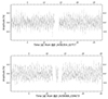 |
Fig. 1. Reduced TESS lighcurves. Top: lightcurve from S2 processed following the recipe of Nardiello et al. (2020, 2021) on the SAP lightcurve (see text). Bottom: same as the top panel but for S29. The typical error on the relative flux is 10−6%, for a maximum variation of ∼0.8% of the mean brightness of the star. |
2.2. CHEOPS photometry
We observed HR 10 using three long-duration visits by CHEOPS (Benz et al. 2021) in October and November 2020 (CHEOPS programme CH_PR1000102; see observation log in Table 1). Each visit lasted about 49 h (∼30 orbits) with an efficiency (fraction of time on target) ranging from 60% to 90%. Exposures were kept short at 3 s in order to enable fast cadence to resolve potential rapid variability. In addition to the subarrays of 100 pix radius that are co-added on board in groups of 14 to save bandwidth, imagettes of 30 pix radius were downlinked at a full 3 s cadence. The CHEOPS automatic data reduction pipeline (Hoyer et al. 2020) does not extract photometry from the imagettes, so we used the point-spread function photometry package PIPE3 developed specifically for CHEOPS (Brandeker et al., in prep.; see also descriptions in Szabó et al. 2021 and Morris et al. 2021). The CHEOPS lightcurves, corrected from roll angle effects, is shown in Fig. 2. We estimated the noise performance of CHEOPS for this G = 6.2 mag star to be 67 ppm over 1 min bins.
Logs of CHEOPS observations.
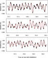 |
Fig. 2. CHEOPS PIPE data corrected for roll angle systematics. The three visits are shown in the top, middle, and bottom panels, respectively. The red line shows a multiperiodic solution of the observations, with frequencies determined from TESS data and free amplitudes (Sect. 4). The typical error bars are on the order of ±15 ppm, and the maximum deviations are on the order of ±40 ppm. |
3. Stellar characterisation
Due to the only recent characterisation of HR 10 as a binary, M19 is the only study to have derived stellar parameters for the two components. Table 2 lists some of the properties for the binary and its individual stellar components. The stellar effective temperatures, Teff, and surface gravity, log g, were obtained by imposing that the combination of the two theoretical stellar atmosphere spectra reproduced first the observed spectra and photometric colours, and in a second step, the spectral energy distribution (SED). The authors used the Gaia DR2 Gaia EDR2 determination of the distance to the system, which is d = 145.18 ± 2.50 pc. However, the Gaia EDR3 Gaia EDR3 distance revision gives d = 102.90 ± 1.56 pc, a reduction by almost a third. With the new value, the luminosities are correspondingly lower, down to LA = 28.79 ± 0.87 L⊙ and LB = 6.88 ± 0.21 L⊙, based on L = 4πFobsd2. The flux Fobs received at Earth, is obtained from the SED fitting by M194. The new luminosities obtained with the DR3 parallax will also affect the surface gravities. The impact on the log g can be estimated by evaluating the shift in values involved by the change in luminosity based on placement comparison with evolutionnary tracks in a Teff − L HR diagram. The corresponding values for log g are then 4.1 and 4.4 for the A and B components, respectively. We prefer to remain conservative on the error bar on this parameter and keep the 0.1 dex one from M19, which was obtained from a fit to spectral lines.
Orbital and stellar parameters of the system.
The new parallax determination clearly impacts the location of the two stellar components (in particular for the primary star) in Hertzsprung–Russell diagrams, as shown in Fig. 3. With the revision, the two members of the binary are clearly within the main sequence of stars with similar masses. This revision could lift up the question whether HR 10 A is in a more evolved subgiant phase, which was implied by the higher estimate of its luminosity (see discussion on the stellar modelling in the next section).
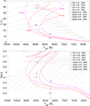 |
Fig. 3. HR diagram positions of the HR 10 system. Top: stellar evolutionary tracks (grey dashed lines) as a function of Teff and L for models from 1.4 to 2.5 M⊙ (by step of 0.1 M⊙). The models are computed with solar initial metallicity and overshooting of αov = 0.05 or 0.10, depending on the mass. The symbols denote the location of HR 10 A and B, respectively, according to M19 (Gaia DR2 parallax for the luminosity, see text) in green, and with the values of L that we revised with the DR3 parallax in blue. The red and purple symbols represent the locations following the stellar parameters of HR 10 A and B modelled as single stars with the CLES code, as reported in Table 3. Isochrones computed with PARSEC1 v1.2S are also depicted, with their ages indicated in the figure. The isochrones in red were computed with the same initial metallicity as the best-fit models obtained in the DR3 case, and selecting two ages enclosing those of the best-fit models. The purple isochrones were obtained with initial metallicities corresponding to that of the best-fit models in the DR2 case. Bottom: same as top panel, but as a function of Teff and log g. |
Given the consequences of the parallax revision for the determination of the evolutionary status of the system, it merits a closer look. In the early release of the Gaia DR3, the renormalised unit weight error (RUWE) parameter was given to measure the quality of the astrometric solution. Despite the length of the collected data series was increased by 12 months, the RUWE parameter for this target has deteriorated from DR2 (RUWE = 1.34) to DR3 (RUWE = 2.74). Moreover, the RUWE index should be around 1 for stars where a single-star model is a good fit to the astrometric data. As mentioned in the EDR3, an index significantly higher should acts as a caution that the target source could be a non-single object. In particular, Kervella et al. (2022) mention the threshold of the RUWE index > 1.4 as indicating a degraded solution mostly from partially resolved binaries. These authors indicate that astrometric solutions with RUWE up to 2–3 can still be considered but with caution. Fitton et al. (2022) discuss the particular case of systems presenting a material disc, for which they recommend to consider a RUWE threshold of 2.4 as an indication of an unresolved binary. This strengthens the origin of the high value of the DR3 RUWE of HR 10 from its non-treated binarity in the current Gaia catalogues. Both DR2 and DR3 RUWE indexes indicate that the Gaia parallaxes of this system should be treated with caution. In the absence of better parallax estimation, we decided to carry out parallel stellar modelling, respectively considering luminosities derived from DR2 and DR3 parallaxes.
3.1. Stellar modelling
We performed a new series of stellar modellings of the two stars. We considered as constraints for the modelling, parameters obtained with the DR2 parallax, and in a second time, a revised parameter set based on the DR3 one. In each case, we made the computations following two scenarios: (1) each star is evolved as a single star; (2) stars were evolved as a binary by imposing they had the same initial chemical composition and reached the same age.
The theoretical models used for the stellar modellings were computed with the Liège stellar evolution code, CLES (Scuflaire et al. 2008). We used the standard solar chemical composition of Asplund et al. (2009), and corresponding opacity tables made with the OPAL library (Iglesias & Rogers 1996). The conditions at the photosphere were obtained from Eddington’s grey law for the atmosphere. We treated convection following the mixing-length theory, implemented as in Cox & Giuli (1968), with its parameter fixed to αMLT = 1.82, following a solar calibration. We included microscopic diffusion with coefficients derived from the resolution of Burgers’ equations following Thoul et al. (1994). Convective overshooting was considered, imposing a difference of αov = 0.05 (expressed in terms of local pressure scaleheights) between the A and B components.
Stellar modelling of HR 10 A and HR 10 B assumed as single stars (S) or as a binary (B), as indicated in the parameter column.
The stellar modelling followed an optimisation scheme aiming at finding the stellar models that best reproduce the observational constraints. The scheme was based on the Levenberg-Marquardt non-linear least square method, which implementation details are presented in Salmon et al. (2021). The code can model simultaneously stars of a multiple system. In this case, the initial composition and the age reached by each modelled star must be the same.
The set of observational constraints were taken in every case as {Teff, log g,L}, following the values given in Table 2. As it was discussed in Sect. 3, the parallax determination for this system is uncertain, impacting the luminosity determination. We thus made two series of stellar modelling; first considering the DR2 luminosities as constraints, LA = 57.30 ± 2 L⊙ and LB = 13.70 ± 0.50 L⊙; then DR3 luminosities LA = 28.79 ± 0.87 L⊙ and LB = 6.88 ± 0.21 L⊙, and correspondingly adapted log g.
3.1.1. Results based on DR2
Based on the DR2 observed parameters, we inferred two sets of ages, masses and metallicities for HR 10 A and B; either from a modelling with each components evolved as single stars [S] or as a common-formed system [B]. The results are given in Table 3. The B solution is not very reliable, as we never succeeded to get a low value of the χ2 function used for measuring the significance of the fit. The convergence of the optimisation scheme for the A component in particular was poor. Indeed, the luminosity constraint pushed the solution towards high masses, which, by imposing same age and initial metallicity, conflicted with the set of constraints for the B star. In the S scenario, the fit of the primary star gave a better result. The location of the two models obtained in this S fit are shown in Fig. 3; they reproduce the observed Teff and L of the two stars. Either in the S or B scenario, the mass estimates for the A and B components are significantly larger than those derived from the orbital solution; HR10 A appears to be in the early stage of the subgiant phase, with the S fit yielding an estimated value of its radius of R ≃ 3.18 R⊙.
3.1.2. Results based on DR3
In this second series, we used the same observational constraints, except they are derived with help of the DR3 parallax. In comparison to the DR2 modelling, the results when stars are evolved as single objects, give older estimates of the ages, around 700–900 Myr, and with a chemical composition significantly subsolar (see Table 3). The location of the two DR3 best-fit models in the S case, are also depicted in Fig. 3. For each star, the log g resulting from the modelling support the increase expected from the downward revision of the luminosities. The mass for the A component is in good agreement with the orbital solution while we predict a lower mass for the secondary component. The age and initial chemical composition do not match exactly between the two stars as we would expect from a binary system.
We again faced more difficulty in modelling the stars as a binary. Results in Table 3 for the B case, point towards a younger age estimate of the system, of 400 Myr. However, the χ2 indicates, as in the DR2 case, that the quality of the fit in this binary scenario is poor. The solution is again degraded by the modelling of the A component, whose Teff is hotter by ∼700 K than the observed one given as a constraint.
3.2. Stellar modelling result synthesis
For the DR2 and DR3 sets of constraints, we also carried out modelling with the help of isochronal mass and age estimates. We employed the isochrone placement technique (see Bonfanti et al. 2015, 2016) in combination with PARSEC1 v1.2S evolutionary models from Marigo et al. (2017). The components were only modelled as single stars, with the same set of constraints as above. With the DR2 luminosities, we get for the primary star M = 2.40 ± 0.04 M⊙ and an age of 494 ± 183 Myr, and for the secondary one M = 1.81 ± 0.04 M⊙ and an age of 608 ± 165 Myr. Both are in agreement with the values we estimated in our first approach, and in particular the primary also appears in the early subgiant phase. Considering the DR3 luminosities, we also obtained results in good agreement with our first series of modelling, finding for the primary M = 2.09 ± 0.09 M⊙ and an age of 550 ± 170 Myr, and for the secondary, M = 1.50 ± 0.06 M⊙ but quite a younger estimate of 150 ± 150 Myr old.
In summary, the results obtained with the DR2 parallaxes reproduce the observed fundamental parameters, Teff, L, and log g but systematically lead to masses larger than those from the orbital solution. With the DR3 parallaxes, the masses inferred are in better agreement with the orbital solution due to the reduction in the luminosity values. In the following sections of this paper, we consider the results based on the stars modelled as single stars. We distinguish the results based on DR2 or DR3, given the difference in the stellar evolution stage of the primary component they imply.
4. Signature of δ Scuti pulsations
We first examined the frequency content of sectors 2 and 29 of TESS. Figure 4 (top curves of each panel) shows the Lomb-Scargle Periodogram (LSP) of the S2 (top) and S29 (bottom), which clearly reveals peaks with significant amplitudes in the range ∼13–817 μHz. Beyond and up to the Nyquist frequency of ∼4166 μHz, the LSP is entirely consistent with noise. We extracted the peak properties (frequency, amplitude, and phase) using the prewhitening technique (Deeming 1975), the standard technique to extract oscillation properties in heat-driven pulsators, with the dedicated software FELIX (Charpinet et al. 2010; Zong et al. 2016). The prewhitening technique consists in subtracting sequentially from the lightcurve each periodic variation spotted above a predefined threshold, defined as a given level of signal-to-noise ratio (S/N). That is, FELIX identifies in the LSP of the lightcurve the frequency, phase, and amplitude of the highest-amplitude peak, which are used as initial guesses in a subsequent non-linear least square (NLLS) fit of a cosine wave5 in time domain using the Levenberg-Marquardt algorithm. The fitted wave of derived frequency, amplitude, and phase is then subtracted from the lightcurve. The operation was repeated as long as there was a peak above the predefined threshold. From the extraction of the second peak and beyond, the model is reevaluated at each step by a simultaneous fit of all the extracted peaks to reevaluate their frequency, phase, and amplitude.
 |
Fig. 4. LSP of TESS lighcurves. Top: LSP of the TESS S2 lightcurve. Bottom: same as the top panel but for S29. The red dashed line indicates the S/N = 5.0 threshold. The top curve shows the LSP computed from the corresponding TESS light curve. Each small vertical blue segment indicates a frequency extracted during the prewhitening. The frequencies and their properties are listed in Tables A.1 and A.2. The curve plotted upside down is a reconstruction of the LSP based on the data summarised in this table, and the curve at the bottom (shifted vertically by an arbitrary amount for visibility) is the residual containing only noise after removing all the signal from the light curve. |
The S/N = 1 level – the noise – is defined locally as the median of the points within a gliding window (centred on each point of the LSP) of 300 times the resolution of the data. This median is reevaluated at each step of the prewhitening, that is each time a peak is removed. The minimum significance that we allow for identifying a peak to remove is 4σ, meaning a false alarm probability of 3.2 × 10⁻⁵ (99.99994% probability that the signal is real). This 4σ significance level can be converted into an S/N = x level. To determine the value of x, we used the approach developed in Zong et al. (2016): using the same time sampling and the same window as in the TESS lightcurves, we simulated 10 000 pure Gaussian white noise lightcurves. For a given S/N threshold we then searched for the number of times that at least one peak in the LSP of these artificial light curves (that are by construction just noise) happen to be above this threshold. We obtained the false alarm probability by dividing by the number of tests (10 000 here). We found that the threshold corresponding to a 4σ significance (false alarm probability of 3.2 × 10⁻⁵), is S/N = 5.0 for both S2 and S29. The lists of peaks extracted down to S/N = 5.0 is given in Appendix A.1: 41 peaks were extracted in S2 down to S/N = 5.0, while for S29, of higher photometric quality, 62 peaks were present down to this threshold. The upside-down curves in Fig. 4 are the reconstruction of the LSP based on these extracted peaks only (top panel for S2 and bottom panel for S29), and the curve at the bottom of each panel of Fig. 4 is the residual containing only noise after removing all the signal from the light curve. No peak above the S/N = 5.0 threshold is left in this residual.
4.1. Interpretation of the frequency peaks
From ∼13.5 to 817.5 μHz, these peaks are consistent with stellar oscillations6, in particular with the frequency domain and properties of δ Scuti pulsation modes, as usually observed from space by photometry (e.g. Balona & Dziembowski 2011; Michel et al. 2017; Antoci et al. 2019). We show in Fig. 5 (top panel) the time–frequency behaviour of the peaks in S29, from gliding windows of 3 days in length with steps of 0.25 d. Main peaks exhibit a stable amplitude and frequency over the length of the data and are therefore like coherent pulsations. Given the frequency in consideration, the dominant peak f1 and close frequencies are very likely of δ Scuti type, which frequencies are usually between 58 and 580 μHz (e.g. Rodríguez et al. 2000).
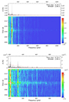 |
Fig. 5. Time–frequency diagram of the peaks in S29, from gliding windows of 3 days in size by steps of 0.25 d. Top: 0–1000 μHz region. Bottom: zoom onto the 200–800 μHz region. The red dashed lines in the upper panels indicate the S/N = 5.0 threshold. |
The second-highest amplitude peak, f2, is around 17.7 μHz. This high-amplitude peak looks much like a feature now often observed in A- and F-type stars (including δ Scuti and γ Dor pulsators) as reported in Balona (2011, 2013, 2017), Trust et al. (2020), Santos et al. (2021). A similar feature was found for the WASP-189 system, based on data from CHEOPS (Deline et al. 2022). Spots from magnetic activity are advanced as one possible cause of the surface modulation thought to be at the origin of these detected high-amplitude periodic signals. Despite the limited extent of the convective surface or subsurface convective regions in A-type stars, Cantiello & Braithwaite (2019) propose they could generate weak magnetic fields by dynamo, leading to surface spots. In that case, the frequency associated with the phenomenon would be an indicator of the stellar surface rotation rate. More recently, an alternative explanation was developed in Lee & Saio (2020) and Lee (2022), who propose the modulation arises from oscillation mode(s). The surface oscillation would result from the resonance between convective modes from the stellar core and classical gravity modes propagating in the radiative near-core and envelope layers. The frequency detected would in that case be indicative of the core rotation rate.
We can compare the frequency of this peak with that derived for the A component with help of its surface velocity, inclination of the system and radii we derived from our stellar modellings.
With the radius from the model of HR 10 A as a single star derived in Sect. 3.1 and the DR2 luminosity, R = 3.21 R⊙, and assuming the stellar equator is coplanar with the orbital plane, we would expect a surface rotation frequency of ∼20.79 μHz. It does not reproduce the f2 peak value, but does not exclude the possibility, given the assumptions we made, that in this case the frequency could correspond to the surface rotation of the primary star. With the results of the DR3 modelling, we got R = 2.23 R⊙, which suggests a surface rotation frequency of ∼30.2 μHz. This clearly does not coincide with the frequency of the f2 peak. The origin of this peak thus cannot be directly confirmed to be related to the stellar surface rotation from the A component (nor the B component actually), though it neither excludes it.
The behaviour of high-frequency peaks, beyond 200 μHz, is shown on the bottom panel of Fig. 5. For these peaks, grouped around ∼217 μHz, ∼324 μHz, and ∼612 μHz, the amplitude seems to vary more significantly during the 27-d data. The amplitude modulation has been reported in many occasions for δ Scuti pulsators (e.g. Breger & Pamyatnykh 2006; Barceló Forteza et al. 2015; Bowman et al. 2016). It is thought to result from resonant mode coupling, leading to non-linear effects and so modulation of the amplitudes. In the high-frequency domain, above the usual δ Scuti regime, there is a debate about the possibility for these modes with time-varying amplitudes to be stochastic solar-like oscillations. The convective region at the surface of δ Scuti stars is expected to be very thin or absent for the hottest ones, and thus unlikely to favour conditions for stochastic oscillations. Presently, no firm evidence could confirm the existence of such modes in δ Scuti stars (Antoci et al. 2013).
4.2. Origin of the stellar pulsations
Identifying which stellar component is the host of the δ Scuti pulsations is not immediate. The primary star is a natural candidate given it is 4.2 times more luminous than its companion. However, its effective temperature, 9000 K, makes it hard to explain the excitation of pulsations since it locates it just out of the hot (blue) border of the δ Scuti instability strip (Dupret et al. 2004). In this region of the instability domain, it is the κ mechanism from the HeII ionisation opacity peak that mostly contributes to the driving of the pulsations. This mechanism is particularly sensitive to Teff, since it is the depth of the peak (which occurs at fixed temperature) that determines whether pulsations can be efficiently driven.
If we first consider the results of our stellar modelling with the DR2 parallaxes, the increase in radius as the star has started is subgiant phase leads to a redistributed thermal stratification in the surface layers. Given the sensibility of conditions for the κ mechanism to work efficiently, the stellar properties of the primary component in this case are not favourable for excitation of δ Scuti pulsations.
The results from the stellar modelling with the DR3 parallaxes indicated that the primary star was most likely in the main sequence. We hence computed with the MAD non-adiabatic code (same code as in Dupret et al. 2004) the pulsations for this model of HR 10 A. We find a very few modes to be excited, meaning the model is marginally predicting pulsations. Michel et al. (2017) reported for a large sample of δ Scuti stars observed by the space-photometry CoRoT mission that the modes with the highest amplitudes range between 0.05 and 3%. The dominant amplitude in our case is ∼0.20%, which if attributed to the primary component (in the DR3 case) is thus in line with CoRoT results.
Nevertheless, given the luminosity difference between the A and B components of HR10 and the possibility for δ Scuti mode amplitudes to reach a few percent, it is also plausible that the pulsations are hosted in the secondary star (either assuming the DR2 or DR3 luminosities).
Finally, in the absence of identification of regularities (large frequency separation) and mode identification, the detected frequencies are difficult to exploit to improve the characterisation of the star hosting them.
5. Investigation of the origin of the flicker noise
5.1. Power spectral density
To compute the power spectral density (PSD) of both CHEOPS and TESS observations, we used the classical periodogram (Schuster 1898) defined as:
with X(tj) the target lightcurve, Δt the time sampling (Δt = 3 seconds for CHEOPS, 120 seconds for TESS), N the number of data points, and ν the Fourier frequencies  defined for
  . Periodogram P is expressed in units of density (ppm2/μHz) by dividing expression (1) by the passband 1/Δt (see Eq. (11.6), Chap. 11 Percival et al. 1994). As both CHEOPS and TESS observations are affected by short data gaps, we follow standard procedure (see, e.g., Appourchaux et al. 2008; Kallinger & Matthews 2010), and fill these gaps using local linear interpolations7. The resulting periodogram of the first CHEOPS visit (see Sect. 2.2) – cleaned by the CHEOPS systematics – and of the second TESS sector (see Sect. 2.1) are shown in Fig. 6. We see in the TESS periodogram clear power excesses around 20, between 70 and 80 μHz, which correspond respectively to the f2 and f1 frequency peaks we reported and discussed in Sect. 4. Other excesses appear at frequencies we identified as δ Scuti pulsations. We note that corresponding power excesses are present in the CHEOPS periodogram, also revealing the detection of the pulsations in the CHEOPS lightcurve. In both cases, we observe a power increase towards the low frequencies. Following the classical terminology, we call this noise component a “flicker noise”. The purpose of this section is to determine the origin of this “flicker” noise. Since this noise is similarly observed in CHEOPS and TESS periodograms, we logically exclude an instrumental origin.
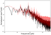 |
Fig. 6. Periodograms of the data taken during the first CHEOPS visit (black, prewhitened by CHEOPS systematics), and periodogram of the data taken during sector 29 of TESS (red). |
A first scenario to explain the flicker noise is related to the stellar companion recently discovered by M19. Since it is cooler in effective temperature, the star is expected to present a larger convective surface region, favouring the possibility of detecting granulation signature at its surface. However, we checked the extent of the convective envelope in the stellar models (in the assumption of single star evolutions) we derived in Sect. 3.1. We found that both for the A and B components, considering either the DR2 or DR3 case, the extent is every time similar, of ∼0.001r/R. Moreover, as we mentioned, the difference between the luminosities (a factor more than 4) of the two stars makes it less likely to detect prominent features from the B component in their non-resolved photometry.
A second scenario is related to the stellar activity of the main star. Indeed, the power increase towards the low frequencies is a common, well-studied, signature of stellar granulation. The granules at the stellar surface evolve with time (from some minutes to years depending on the spectral type) and generate stochastic (but correlated) photometric fluctuations over a wide range of amplitudes and timescales. It has been first well identified on the Sun (Harvey 1985; Palle et al. 1995), but also in red-giants (Balona & Dziembowski 2011) or main-sequence stars using Kepler (see e.g., Bastien et al. 2013; Kallinger et al. 2014; Cranmer et al. 2014; Pande et al. 2018; Sulis et al. 2020), and recently using CHEOPS data (Delrez et al. 2021; Sulis et al. 2023). Stellar granulation has also been identified as the potential driver for the photometric fluctuations observed on the cooler population of A stars (≤7500 K, see e.g., Balona 2011). However, for the population of the hotter A-type stars – where HR 10 stands (assuming its effective temperature of 9000 ± 100 K is correct) – the existence of any measurable signature of surface convection received mixed support (Balona & Dziembowski 2011) as this convective zone is extremely thin. In Kallinger & Matthews (2010), the observed flicker noise of two A2 stars (Teff = 8080 ± 160 K and 7500 ± 200 K) has been attributed to stellar granulation based on the argument that the amplitude of the stellar granulation photometric signature is dependent on the total number of granulation cells on the stellar surface and not on the depth of the convection zone. Moreover, Landstreet et al. (2009) established from spectroscopy of A stars clear signatures (from non-zero values of the micro-turbulence parameter, and reversed C-shaped bisectors for the asymmetric absorption line profiles) of local atmospheric velocity fields, confidently linked to atmospheric convection, for stars cooler than 10 000 K. To our knowledge, there is no reported detection of stellar granulation from photometric data for stars as hot as HR 10. Below, we present an investigation of whether or not the stellar granulation can explain the observed flicker noise.
5.2. Investigating stellar granulation as a plausible source for the flicker noise
For main sequence and giant stars, it has been shown that the root mean square (RMS) of their brightness variation evaluated over a timescale between 0.5 and 8 h (called the “8-h flicker”, or simply “F8”) is driven by stellar granulation. As a consequence, the F8 measurement correlates with their stellar surface gravity and allows a rough measurement of this stellar fundamental parameter without asteroseismology or spectroscopy analyses (Bastien et al. 2013, 2016). As the log g value of HR 10 was obtained by M19 through spectroscopy analyses (see Table 2), we compare this value with the F8 scaling predictions. To compute F8, we follow the recipe explained in Bastien et al. (2013): we binned the individual CHEOPS visits into 30 min intervals and used a 16 points boxcar filter to remove the long-term activity at periods > 8 h. We obtain F8 = [2489, 2854, 2428] ppm, respectively for the three CHEOPS visits. Then, because CHEOPS and Kepler passbands are similar8, we correct for the influence of the photon noise by applying Eq. (3) of Bastien et al. (2016) with the mean value ⟨F8⟩ = 2590.75 ppm. We obtain log g = 3.8 using the F8 scaling predictions, which is in total agreement with the value derived by M19 (see Table 2) based on DR2. It is therefore in favour of a granulation-driven flicker noise. This result also appears to disfavour the surface gravity revision implied by the DR3 parallax.
For main sequence stars, it has also been shown that the periodogram slope (also referred to as the flicker index) measured on the frequency range corresponding to stellar granulation is correlated with the stellar fundamental parameters, and particularly with the stellar surface gravity (Sulis et al. 2020, 2023). We evaluate as a second test if the flicker indexes measured on CHEOPS and TESS periodograms follow the expected correlations that have been observed with the log g. For that purpose, we first removed in the CHEOPS and TESS lightcurves from the most significant stellar oscillations periodic signatures (using the prewhitening technique as in Sect. 4, as they can perturb the measurement of the periodogram slopes). The prewhitening method produces residuals lightcurves, to which we apply local linear interpolations to fill the gaps (as done in Sect. 5.1). The resulting periodograms of the first CHEOPS visits and the sector 29 of TESS are shown in Fig. 7. We divide them into 1 day time series to compute the averaged periodograms from which we infer the flicker index, as this allows to reduce the variance at a given frequency. The averaged periodogram is defined as:
with P given by Eq. (1) and L the number of available subseries (L = 2 for CHEOPS first visit, L = 25 for TESS sector 29). The resulting averaged periodograms are shown in red in Fig. 7. From these periodograms, we can visually see three different power regimes: one at high frequencies (ν ⪆ 2000 μHz for CHEOPS, and ν ⪆ 1000 μHz for TESS), one that we defined as the flicker noise regime (between the blue vertical dashed lines), and one at low frequencies (ν ⪅ 200 μHz for both CHEOPS for TESS). As in Pallé et al. (1999) and Sulis et al. (2020), we choose to represent the noise correlations in these three different regimes by using simple models based on 1/να power laws of the form:

Therefore, model (3) contains 8 free parameters (indexes α and amplitudes β for each three regimes, plus two cut-off frequencies {fg, fH} that mark these three regimes out). We fit model of Eq. (3) to the averaged periodograms from Eq. (2) of CHEOPS and TESS data with the same Markov Chain Monte Carlo (MCMC) numerical scheme as described in Sect. 4.2 of Sulis et al. (2020). The starting values were set to the visual determination of the cut-off frequencies and no prior were used. Results for the flicker noise are listed in Table 4. We obtain comparable flicker indexes for CHEOPS (αg = 2.09 ± 0.15) and TESS data (2.07 ± 0.09). Since the high-frequency noise component is higher in TESS data than in CHEOPS, it dominates a larger frequency region of the periodogram and masks the highest component of the flicker noise leading to fH inferred from TESS averaged periodogram that is lower than from CHEOPS averaged periodogram. In return, the lower cut-off frequencies fg derived on both dataset are consistent within their error bars. Comparing the flicker indexes measured on HR 10 periodograms with the ones derived from Kepler data in Sulis et al. (2020), we observe a good match with the expectation from main-sequence and giant stars9 (see Fig. 8). This is again in favour of a granulation-driven flicker noise.
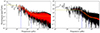 |
Fig. 7. Periodograms of CHEOPS and TESS lightcurves. Left: Periodogram of the first CHEOPS visit prewhitened by the significant oscillations (black), and averaged periodogram combining two one-day subseries (red). Right: Periodogram of TESS sector 29 prewhitened by the significant oscillations (black), and averaged periodogram combining the 25 available one-day subseries (red). In both panels, best-fitting models resulting from Harvey function fits given by Eq. (4) are shown in yellow. The cut-off frequencies of the flicker noise resulting from the MCMC analyses are indicated by the blue vertical dashed lines. We note the different frequency ranges on the x-axes. |
Flicker noise parameters inferred from the MCMC analyses of both CHEOPS and TESS averaged periodograms.
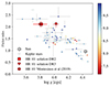 |
Fig. 8. Estimated flicker indexes associated with granulation as a function of the stellar log g for Kepler bright (Kepler magnitude < 10) targets, adapted from Fig. 17 of Sulis et al. (2020). For this comparison, the flicker indexes have been interpolated to correspond to the value that would be measured at a constant level of high-frequency photon noise (here taken at 30 ppm). The quality of this interpolation depends on the level of photon noise, which is directly related to the stellar magnitude (indicated by the colour code). The flicker index inferred from solar VIRGO data (with a white Gaussian noise of 30 ppm standard deviation added) is shown with the solar symbol for reference. The flicker index inferred from HR 10 photometric data (no interpolation needed for this target; see footnote 7) is shown with the square, triangle, and cross symbols adopting log g from stellar modelling with Gaia DR2 data, Gaia DR3 data, and with spectroscopic analysis (M19), respectively (see Table 3). |
As a last test, following Kallinger & Matthews (2010), we compare the granulation characteristic frequency with the atmospheric pressure scale height  that must scale with the average size of the granule cells at the stellar surface and frequency of maximum power, νmax. For that purpose, we model the periodogram in Eq. (1) as the sum of an Harvey function (Harvey 1985) with a single component for granulation and a white Gaussian noise of variance σw2 (for the high frequency noise component). The model reads as,
where the set of parameters {a, bν, c} collects the amplitude, characteristic frequency and power of the Harvey function. Notation νk+ means that positive Fourier frequencies are considered. We perform a least-square fitting procedure to evaluate the best-fitting parameters of model (4) on the averaged periodogram of the prewhitened first visit of CHEOPS and sector 29 of TESS (see yellow lines in Fig. 7). We obtained a granulation characteristic frequency bν = 165.06 μHz in the case of CHEOPS and bν = 150.87 μHz in the case of TESS. These frequencies are shown as a function of the atmospheric pressure scale height in Fig. 9. Both are approximately consistent with the observed trend, and this comparison goes in favour of a granulation-driven flicker noise. However, this has to be tempered regarding the uncertainties that remain on the stellar parameters of the system.
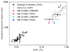 |
Fig. 9. Characteristic granulation frequency (bν) as a function of the stellar atmospheric pressure scale height (computed in solar units) for COROT red giant stars (black). The figure is extracted from Kallinger & Matthews (2010). We added to the original plot the Kepler bright (magnitude < 10) main sequence targets (grey) shown in Fig. 8 and described in Sulis et al. (2020). Frequency bν for HR 10 has been inferred from both the averaged periodograms of the CHEOPS first visit (red, cyan) and TESS sector 29 (magenta, blue), adopting stellar parameters from stellar modelling with Gaia DR2 and DR3. |
We conclude that, albeit not ‘direct’ evidence that the origin of the observed flicker noise is the stellar granulation, the inferred flicker noise characteristics (amplitude F8, correlation ag, and characteristic frequency bν) are consistent with the scaling laws derived from main sequence and giant stars. We see in particular that the flicker noise properties derived with the help of stellar parameters from the DR2 stellar modelling are clearly in line with the trend predicted by scaling laws. Regardless of the stellar properties considered, the results of the present analysis bring into question our current understanding of the properties of surface convection in early-type A dwarf stars.
6. Analysis of transients in the lightcurve
The possible non-periodic transient can be revealed by removing the periodic light curve components. We applied two methods to remove these. At first, following a prewhitening approach, we removed the periodic signals one-by-one, as is done in Sect. 4. We used in particular the list of frequencies extracted in that section to have a first guess of the frequencies of the stellar periodic signals in the CHEOPS lightcurve. The second approach is based on a synthetic curve model that includes a sum of periodic signal and makes vary their free parameters (amplitudes, frequencies,...) until minimising the subtraction of this model to the non-cleaned lightcurve. The two approaches are detailed hereafter.
6.1. A step-by-step removal of frequencies
We first followed the ‘classical’ step-by-step removal of stellar frequencies. The goal of this approach is to reveal the possible transients once all the significant sine-like components are subtracted from the lightcurve. We thus identified the most significant frequency components first as in Sect. 4. We then removed a linear combination of harmonic functions with frequencies that were identified as major contributors in each step.
However, this approach can still lead to the removal of a definite transient. The fitting of frequencies and amplitudes of many harmonic signals can result in mimicking a transient for some values of the amplitudes. Consequently, the probability of a false negative detection is non-zero. This method has the advantage to be considered as not producing false positive results (unless presence of some unrecognised instrument systematics). Hence, in the case of a possible transient detection, it can be considered as conclusive.
6.2. A global solution of lightcurves in a synthesis approach
The possible transients in the lightcurve were sought with signal reconstruction with synthesis. The attempt interprets the measured signal as a sum of a parametric model and residuals, where the residual term is minimised. The main equation of the reconstruction process is:
![$$ \begin{aligned} S&= \left[ {\begin{array}{ccccccc} F(t_1),F(t_2), \ldots , F(t_n) , \\ \end{array} } \right] ^T\end{aligned} $$](/articles/aa/full_html/2024/10/aa46180-23/aa46180-23-eq11.gif)
![$$ \begin{aligned} \mathbf V&=\left[ {\begin{array}{ccccccc} s_1(t_1)&c_1(t_1)&s_2(t_1)&c_2(t_1)&\ldots&c_m(t_1)&T(t_1)\\ s_1(t_2)&c_2(t_2)&s_2(t_2)&c_2(t_1)&\ldots&c_m(t_2)&T(t_1)\\ \ldots&\ldots&\ldots&\ldots&\ldots&\ldots&\ldots \\ s_1(t_n)&c_2(t_n)&s_2(t_n)&c_2(t_n)&\ldots&c_m(t_n)&T(t_n)\\ \end{array} } \right] , \end{aligned} $$](/articles/aa/full_html/2024/10/aa46180-23/aa46180-23-eq12.gif)
![$$ \begin{aligned} A&= \left[ {\begin{array}{ccccccc} As_1&Ac_1&As_2&Ac_2&\ldots&Ac_m&AT\\ \end{array} } \right] ^T , \end{aligned} $$](/articles/aa/full_html/2024/10/aa46180-23/aa46180-23-eq13.gif)
where the signal vector t = ℝn is the vector of times of observations, S = ℝn is the vector composed by the F fluxes sampled according to t; V = ℝ2m + 1, n is the matrix of harmonic templates belonging to the m identified frequencies (s and c describe the sine and cosine parts of the harmonic co-vectors) and Tℝn is a parametric template describing the transit shape. Writing T in the form as T(T0, P, ω, b)(tj) we see that T is a function of the times of the transits, the transit duration and the transit shape, via the ω = (a/RS)(2π/P)(1 − b2)−1/2 scaled duration (see Pál 2009) and the b impact parameter. T does not contain an amplitude term, similarly to all other column vectors in V, because the amplitudes of all parametric components will be assigned by the amplitude vector A = ℝm + 1. The best-fit parametric solution of T is defined at the minimum of χ2, and the component belonging to this reconstruction of the transient is given by the scalar multiplication AT ⋅ T.
In this method, we took the stellar frequencies from the TESS lightcurves (see Tables A.1 and A.2), and calculated basis vectors showing the frequency pattern of these components. We guessed the transient component with randomized parameters and injected it to the component vectors. Then the model described in Eqs. (5–8) were solved with a global linear optimisation, where the amplitudes for all harmonic components and the transient pattern were fitted parameters.
6.3. TESS data
The TESS S2 and S29 photometry and their analysis are shown in Figs. 10 and 11. Data are plotted cut into four parts, consisting of two parts per sector, that is dividing the first and second half of data from S2 and S29, respectively. The panels are ordered in pairs, where the upper panel (black points) show the raw TESS lightcurve, and the lower panels (red dots) show the residuals from a step-by-step frequency subtraction procedure. In this step-by-step procedure, 74 frequencies have been removed from data from both segments. The scatter in the residuals are 584 ppm and 410 ppm, respectively. The scatter in the first and second half of both sectors are different. The residuals in the first and second half of S2 data have a scatter of 560 and 599 ppm, respectively; while in S29, the same analysis results in 399 and 417 ppm in the first and second half of the data. It also has to be noted that the amplitude of the last harmonic component (that had the least fitted amplitude) had an amplitude of 21 ppm in the case of S2, and 16 ppm in the case of S29. The expected noise in the data is read-out-noise-limited, which is 328 ppm for a single exposure at 2 min cadence (Ricker et al. 2015).
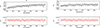 |
Fig. 10. TESS Sector 2 observations of HR 10. Top row: measured lightcurve. Bottom row: residuals after subtracting the frequencies to 4σ significance (S/N = 5.0). The panels are ordered in pairs, where the upper panels (black points) show the raw TESS lightcurve, and the lower panels (red dots) show the residuals from a step-by-step frequency-subtraction procedure. |
We interpret the varying level of residuals as signs of additional non-periodic lightcurve components. This interpretation is further strengthened by the visually apparent structures especially in the S2 residuals. Even, the residuals appear to suggest a periodic or quasi-periodic component with a characteristic period of 2.5 days, and probably additional instabilities. The presence of similar structures is less apparent in the S29 residuals, which is compatible to the decreased level of noise in the residuals as well. However, the noise in S29 still exceeds the noise budget consisting of the read out noise, the photometry noise and the noise from frequency components in the data below 16 ppm amplitude.
The presence of these structures and noise components also introduce a bias in estimating the frequencies and amplitudes of each periodic components. These biases lead to a slightly mis-estimated pulsation pattern; and lead to apparently time-dependent pulsation frequencies and amplitudes, mostly changing in the timescale of many hours to several days10. Indeed, this has been observed in the case of lightcurve residuals. In small analysis windows on the time domain, the periodic model of the lightcurve has led to surprisingly small residuals; while the frequency and the amplitude of the different modes were unrealistically biased.
These issues can be at least partly eliminated with the lightcurve synthesis approach. Following the recipe described in Eqs. (5–8), we defined a trial signal with free parameters involving the period, duration and time parameters. (The depth of the signal is part of the solution itself, and it is not a free parameter in this approach.) During this analysis, we found that the residuals in TESS S2 data can be interpreted to be periodic, with a tentative periodicity of 2.46 days (Fig. 12, upper panel). The amplitude of the presumed anomalies decrease from 500 ppm amplitude in the data window before the data download gap, and it is only barely visible in the data after the gap. After TBJD 2458354.747, the presumed periodical residuals completely disappeared, and the residuals are below 100 ppm everywhere (Fig. 12, lower panel). The shape of the found anomaly is asymmetric and has some resemblance to the well-known shark-fin shaped anomalies due to exocomets in the β Pic system (Lecavelier des Etangs 2022), which is compatible to the interpretation that in case of HR 10, the anomaly may also mark a diffuse structure which disappeared after a few orbits.
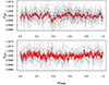 |
Fig. 12. Phased lightcurves of residuals in TESS S2 data after removing the frequencies to the 4σ limit (S/N = 5.0). The period is 2.46 days, the epoch is BJD 2457000.0. Upper panel: points between 2458354.115 and 2458369.746. Lower panel: points between 2458354.747 and 2458381.519. |
We find no evident residuals in the S29 data of HR 10, which were taken before the CHEOPS observations, but were published after the completion of the three CHEOPS visits of HR 10. We decided to include HR 10 into the CHEOPS GTO program because of the residuals in TESS S2 data, with the intention of confirming the transient residuals in the lightcurve. We discuss the analysis of CHEOPS data hereafter.
6.4. CHEOPS photometry
The aim of the CHEOPS observations was to confirm the temporal presence of these suspected transients in the TESS lightcurve. In general, we followed the same steps in the analysis as in the case of the TESS observations. Here we followed the step-by-step frequency removal strategy, and tried both of the two possible approaches. Because the CHEOPS lightcurve covered a shorter time span (3 × 30 CHEOPS orbits) than the TESS observations, it was possible to take the pulsation frequencies from the TESS determination, and refit their amplitudes and phases in case of CHEOPS data. The other possibility is to derive the pulsation frequencies from CHEOPS data as well, and just later compare it to the TESS frequencies. Because two years have passed between TESS S2 data and the CHEOPS observations, and some modes of a few δ Scuti stars are known to vary (Breger 2009), we keep the approach of deriving the full frequency model from CHEOPS data, and later compared it to the TESS analysis. This determination, noteworthy, has proven that all important pulsation component above an S/N > 5.0 limit were completely compatible between TESS and CHEOPS measurements. Because the frequencies were well defined even in the CHEOPS data, although spanning on a much shorter time range than the TESS ones, the two approach gave practically identical results. We now describe the method for cleaning from the pulsation found from the CHEOPS data.
Clearing up the data for pulsation patterns is a one-parameter problem in this approach, where the parameter is the significance level of frequencies that we still involve into the periodic model. We examined three frequency cuts, at S/N limits of 11.0, 8.0, and 5.1 (S/N = 5.1 corresponding to a 4σ significance in CHEOPS data, following the same procedure to evaluate the S/N level as a function of FAP/σ-level significance as in Section 4); where the smaller S/N thresholds correspond to more extensive cleaning. We experienced that the residuals behaved similarly, and the most prominent residuals were found in case of the second CHEOPS visit. Somewhat surprisingly, the more periodic components were involved in the frequency cleaning the higher S/N the residuals had, understood as the amplitude of the smoothed residuals divided by the its scatter. This can be an evidence for the real presence of a temporal non-periodic process superimposed to the pulsation pattern. We show the results after a frequency removal with a threshold of peak S/N > 5.1 in Fig. 13. With a more extreme cleaning, which is when the step-by-step method was applied to the three CHEOPS chunks individually (the phases and amplitudes were independently fitted within the individual two-day CHEOPS visits), no significant residuals survived (however, the physical plausibility of such cleaning is questionable, because the modes are expected to be stable on the timescale of two weeks).
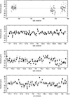 |
Fig. 13. Step-by-step analysis of the CHEOPS data processed with PIPE and removing the frequencies identified in the CHEOPS data one by one. The top panel depicts the three CHEOPS visits together, while the three bottom panels each represent the isolated visits. |
There are two purposes to this step: removal of the periodic pattern from the lightcurve, and a means to identify the main pulsational frequencies for an asteroseismic analysis. The applied definition of the threshold level, which takes the S/N as the selection criterion, optimally supports the removal of the periodic components, as this develops the pattern clearing towards the gradient of the standard deviation of the light curve. This is why we decided to use this method, which is also widespread and well-tested. A possible alternative is based on the false alarm probability (FAP) of each of the frequencies, which is usually obtained using a bootstrap evaluation of the residuals after the removal of each frequency, such as in Szabó et al. (2013). Another alternative is to analyse the Lomb-Scargle periodograms instead of the Fourier transforms. It is important to note that the two methods (the S/N and the FAP threshold) are expected to lead to the same result if the noise follows a normal distribution. This criterion is merely fulfilled after the main frequencies have been removed, because the instrumental noise components of CHEOPS can be reasonably assumed to follow a normal distribution (Maxted et al. 2022). If there are differences in the prioritization of the low-amplitude peaks, the S/N criterion cleans up more periodic components and leads to a clearer view of the non-periodic signal (‘clearer’ in the sense that the features appear in a less noisy background). This comes with the absolutely harmless cost of a somehow fuzzy cut-off of frequencies as it would be observed in the FAP space. But due to an S/N threshold at 5.1, this is still in the order of FAP ∼ 10−6. In essence, we do not see any difference between the applied S/N criterion and the alternative FAP-based frequency selections which would impact any of the aspects discussed in this paper.
We can summarise our findings based on the three CHEOPS visits as follows. First, we see no suspicious residuals in the first visit. There are however evident residuals during the second visit with presumably complex structure, and the average flux is also slightly lower, at ∼30 ppm. Finally, we get suspicious residuals in the case of the third visit. Nevertheless, given the low level of suspicious signal in the residuals, and without characteristics features appearing, we cannot identify the source of the signal, and cannot decipher for instance between an exocomet or CS disc inhomogeneity origin.
7. Conclusion
In this study, we reanalysed the HR 10 system based on new photometric data obtained in two TESS sectors and three CHEOPS visits. Thanks to these data, we were able to characterise the stellar origin of photometric variations and improve the modelling of the periodic signals already postulated in previous studies of this system. We then searched for other signals in the residuals of TESS and CHEOPS lightcurves, once corrected for stellar origin variability.
First, we reused the stellar parameters derived in the study of M19, the only study to date in which the system is analysed as a binary. We also revised their determination of the luminosities for the two components, because the parallax of the system was reduced in the Gaia DR3 by one-third. Using the new luminosity values, we find the A component to be in main sequence. However, the higher luminosity values inferred from the DR2 parallax by M19 are also shown to unambiguously lead to the placement of the primary component in the early subgiant phase. The masses of the system in that case are larger than that from the orbital solution. On the contrary, with the revised luminosity estimates, the masses derived through our stellar modelling are in good agreement with those obtained from the orbital solution of M19, although the mass of the secondary appears lower by ∼0.10 − 0.20 M⊙ in some of our models. The question of the parallax determination is thus of central importance for the stellar characterisation of this binary system. The fact that the parallax was treated with a single-star model in the Gaia DR2 and DR3 data reduction treatments encourages us to put renewed effort into the analysis of its astrometric data. We also note that the question of stellar rotation should certainly be considered in the future. For stars of these spectral types, determining fundamental stellar parameters can be complex, especially in the case of fast rotation (e.g. Niemczura et al. 2015). The inclusion of rotation in the stellar models can also have an impact depending on how close a star is to its critical rotational velocity and its stage of evolution.
With the help of the TESS data, we characterised the periodic signals of stellar origin. We clearly identify δ Scuti modes with frequencies between ∼72 and 600 μHz. Moreover, a detailed study of the flicker noise also reveals it has the characteristic properties of granulation one would expect from the presence of stellar surface convection. This is at odds with the near-surface convection regions predicted for A-type stars (Cantiello & Braithwaite 2019), in particular for the hot primary component. Our models of HR 10 A and HR 10 B each present a surface convective zone. However, their extension is limited to less than 0.001 of their radius, and it is difficult to predict whether the presence of the surface convective zone is sufficient to explain a granulation signature in the photometry. A more detailed study of the granule properties based on the flicker noise parameters (as e.g. in Seleznyov et al. 2011) we derived could reveal unsuspected properties on the surface of A-type stars.
We then proceeded to the cleaning of stellar contributuins from the TESS and CHEOPS lightcurves. A suspicious regular event with a period of ∼2.46 d appears in the residuals of the S2 TESS sector, but cannot be found in the S29 sector. In the residuals of two of the CHEOPS visits, residual variability is suspected. Nevertheless, none of this variability could be firmly linked to an exocometary or CS disc origin. As these two features remain open questions, they are an invitation to continue efforts to follow the system, and with more data we may manage to characterise the origin of these transients and planetesimals/comets presence.
CHEOPS data are archived and available at https://dace.unige.ch/cheopsDatabase/
In heat-driven pulsators, the oscillations are coherent over times that are much longer than the duration of the observations, meaning their lifetimes, which are driven by the evolution of the star, are much longer than the duration of the observations. The assumption of an oscillation by a perfectly periodic signal is therefore fully justified.
The impact of the gap interpolation depends on the frequency. For the first visit of CHEOPS, the duty cycle is ∼82% and the typical length of the gaps (for 99.89% of them) is ≤1 min. Therefore, their impact on the periodogram is negligible for periods longer than 2 min. For the sector 29 of TESS, the duty cycle is ∼89.8% and the typical length of the gaps (for 99.97% of them) is ≤5 min, leading to a negligible impact on periods longer than 10 min.
We note that we cannot do the same numerical application with TESS data as Eq. (3) of Bastien et al. (2016) is only valid for instruments with similar passband than Kepler.
Those could also be responsible of the time variation of some pulsation modes we observed in Sect. 4.
Acknowledgments
We have special thanks to address to Dr B. Montesinos, the referee, who gave us very detailed comments and suggestions on the paper. We are indebted to him for having brought to our attention the question of the parallaxes quality assessment in the Gaia DR2 and DR3. We thank Dr V. Antoci for helpful discussion on δ Scuti pulsators. CHEOPS is an ESA mission in partnership with Switzerland with important contributions to the payload and the ground segment from Austria, Belgium, France, Germany, Hungary, Italy, Portugal, Spain, Sweden, and the United Kingdom. The CHEOPS Consortium would like to gratefully acknowledge the support received by all the agencies, offices, universities, and industries involved. Their flexibility and willingness to explore new approaches were essential to the success of this mission. This paper includes data collected by the TESS mission that are publicly available from the Mikulski Archive for Space Telescopes (MAST). Funding for the TESS mission is provided by NASA’s Science Mission directorate. We are grateful to V. Antoci for helpful comments. SJAJS has received funding from the European Research Council (ERC) under the European Union’s Horizon 2020 research and innovation program (grant agreement No 833925, project STAREX). VVG is an F.R.S-FNRS Research Associate. SS acknowledges the support from CNES, the Programme National de Planétologie (PNP), and the Programme National de Physique Stellaire (PNPS) of CNRS-INSU. GyMSz acknowledges the support of the Hungarian National Research, Development and Innovation Office (NKFIH) grant K-125015, a a PRODEX Experiment Agreement No. 4000137122, the Lendület LP2018-7/2021 grant of the Hungarian Academy of Science and the support of the city of Szombathely. ABr was supported by the SNSA. This project has received funding from the European Research Council (ERC) under the European Union’s Horizon 2020 research and innovation programme (project FOUR ACES. SH gratefully acknowledges CNES funding through the grant 837319. SGS acknowledges support from FCT through FCT contract nr. CEECIND/00826/2018 and POPH/FSE (EC). DG gratefully acknowledges financial support from the CRT foundation under Grant No. 2018.2323 “Gaseous or rocky? Unveiling the nature of small worlds”. SC acknowledges financial support from the Centre National d’Etudes Spatiales (CNES, France) and from the Agence Nationale de la Recherche (ANR, France) under grant ANR-17-CE31-0018, funding the INSIDE project. ACC and TW acknowledge support from STFC consolidated grant numbers ST/R000824/1 and ST/V000861/1, and UKSA grant number ST/R003203/1. YAl acknowledges the support of the Swiss National Fund under grant 200020_172746. We acknowledge support from the Spanish Ministry of Science and Innovation and the European Regional Development Fund through grants ESP2016-80435-C2-1-R, ESP2016-80435-C2-2-R, PGC2018-098153-B-C33, PGC2018-098153-B-C31, ESP2017-87676-C5-1-R, MDM-2017-0737 Unidad de Excelencia Maria de Maeztu-Centro de Astrobiología (INTA-CSIC), as well as the support of the Generalitat de Catalunya/CERCA programme. The MOC activities have been supported by the ESA contract No. 4000124370. SCCB acknowledges support from FCT through FCT contracts nr. IF/01312/2014/CP1215/CT0004. XB, SC, DG, MF and JL acknowledge their role as ESA-appointed CHEOPS science team members. LBo, VNa, IPa, GPi, RRa, GSc, VSi, and TZi acknowledge support from CHEOPS ASI-INAF agreement n. 2019-29-HH.0. ACC acknowledges support from STFC consolidated grant numbers ST/R000824/1 and ST/V000861/1, and UKSA grant number ST/R003203/1. PEC is funded by the Austrian Science Fund (FWF) Erwin Schroedinger Fellowship, program J4595-N. This project was supported by the CNES. The Belgian participation to CHEOPS has been supported by the Belgian Federal Science Policy Office (BELSPO) in the framework of the PRODEX Program, and by the University of Liège through an ARC grant for Concerted Research Actions financed by the Wallonia-Brussels Federation. LD is an F.R.S.-FNRS Postdoctoral Researcher. This work was supported by FCT – Fundação para a Ciência e a Tecnologia through national funds and by FEDER through COMPETE2020 – Programa Operacional Competitividade e Internacionalizacão by these grants: UID/FIS/04434/2019, UIDB/04434/2020, UIDP/04434/2020, PTDC/FIS-AST/32113/2017 and POCI-01-0145-FEDER- 032113, PTDC/FIS-AST/28953/2017 and POCI-01-0145-FEDER-028953, PTDC/FIS-AST/28987/2017 and POCI-01-0145-FEDER-028987, O.D.S.D. is supported in the form of work contract (DL 57/2016/CP1364/CT0004) funded by national funds through FCT. B-OD acknowledges support from the Swiss State Secretariat for Education, Research and Innovation (SERI) under contract number MB22.00046. MF and CMP gratefully acknowledge the support of the Swedish National Space Agency (DNR 65/19, 174/18). MG is an F.R.S.-FNRS Senior Research Associate. KGI is the ESA CHEOPS Project Scientist and is responsible for the ESA CHEOPS Guest Observers Programme. She does not participate in, or contribute to, the definition of the Guaranteed Time Programme of the CHEOPS mission through which observations described in this paper have been taken, nor to any aspect of target selection for the programme. This work was granted access to the HPC resources of MesoPSL financed by the Region Ile de France and the project Equip@Meso (reference ANR-10-EQPX-29-01) of the programme Investissements d’Avenir supervised by the Agence Nationale pour la Recherche. ML acknowledges support of the Swiss National Science Foundation under grant number PCEFP2_194576. PM acknowledges support from STFC research grant number ST/M001040/1. This work was also partially supported by a grant from the Simons Foundation (PI Queloz, grant number 327127). IRI acknowledges support from the Spanish Ministry of Science and Innovation and the European Regional Development Fund through grant PGC2018-098153-B- C33, as well as the support of the Generalitat de Catalunya/CERCA programme. NAW acknowledges UKSA grant ST/R004838/1.
References
- Abt, H. A., & Moyd, K. I. 1973, ApJ, 182, 809 [NASA ADS] [CrossRef] [Google Scholar]
- Antoci, V., Handler, G., Grundahl, F., et al. 2013, MNRAS, 435, 1563 [NASA ADS] [CrossRef] [Google Scholar]
- Antoci, V., Cunha, M. S., Bowman, D. M., et al. 2019, MNRAS, 490, 4040 [Google Scholar]
- Appourchaux, T., Michel, E., Auvergne, M., et al. 2008, A&A, 488, 705 [NASA ADS] [CrossRef] [EDP Sciences] [Google Scholar]
- Asplund, M., Grevesse, N., Sauval, A. J., & Scott, P. 2009, ARA&A, 47, 481 [NASA ADS] [CrossRef] [Google Scholar]
- Balona, L. A. 2011, MNRAS, 415, 1691 [NASA ADS] [CrossRef] [Google Scholar]
- Balona, L. A. 2013, MNRAS, 431, 2240 [NASA ADS] [CrossRef] [Google Scholar]
- Balona, L. A. 2017, MNRAS, 467, 1830 [NASA ADS] [CrossRef] [Google Scholar]
- Balona, L. A., & Dziembowski, W. A. 2011, MNRAS, 417, 591 [NASA ADS] [CrossRef] [Google Scholar]
- Barceló Forteza, S., Michel, E., Roca Cortés, T., & García, R. A. 2015, A&A, 579, A133 [NASA ADS] [CrossRef] [EDP Sciences] [Google Scholar]
- Bastien, F. A., Stassun, K. G., Basri, G., & Pepper, J. 2013, Nature, 500, 427 [Google Scholar]
- Bastien, F. A., Stassun, K. G., Basri, G., & Pepper, J. 2016, ApJ, 818, 43 [NASA ADS] [CrossRef] [Google Scholar]
- Benz, W., Broeg, C., Fortier, A., et al. 2021, Exp. Astron., 51, 109 [Google Scholar]
- Beust, H., Lagrange-Henri, A. M., Vidal-Madjar, A., & Ferlet, R. 1990, A&A, 236, 202 [NASA ADS] [Google Scholar]
- Beust, H., Vidal-Madjar, A., & Ferlet, R. 1991, A&A, 247, 505 [NASA ADS] [Google Scholar]
- Bonfanti, A., Ortolani, S., Piotto, G., & Nascimbeni, V. 2015, A&A, 575, A18 [NASA ADS] [CrossRef] [EDP Sciences] [Google Scholar]
- Bonfanti, A., Ortolani, S., & Nascimbeni, V. 2016, A&A, 585, A5 [NASA ADS] [CrossRef] [EDP Sciences] [Google Scholar]
- Bowman, D. M., Kurtz, D. W., Breger, M., Murphy, S. J., & Holdsworth, D. L. 2016, MNRAS, 460, 1970 [NASA ADS] [CrossRef] [Google Scholar]
- Breger, M. 2009, AIP Conf. Ser., 1170, 410 [NASA ADS] [CrossRef] [Google Scholar]
- Breger, M., & Pamyatnykh, A. A. 2006, MNRAS, 368, 571 [NASA ADS] [CrossRef] [Google Scholar]
- Cantiello, M., & Braithwaite, J. 2019, ApJ, 883, 106 [Google Scholar]
- Charpinet, S., Green, E. M., Baglin, A., et al. 2010, A&A, 516, L6 [NASA ADS] [CrossRef] [EDP Sciences] [Google Scholar]
- Cox, J. P., & Giuli, R. T. 1968, Principles of Stellar Structure (New York: Gordon and Breach) [Google Scholar]
- Cranmer, S. R., Bastien, F. A., Stassun, K. G., & Saar, S. H. 2014, ApJ, 781, 124 [CrossRef] [Google Scholar]
- Deeming, T. J. 1975, Ap&SS, 36, 137 [Google Scholar]
- Deline, A., Hooton, M. J., Lendl, M., et al. 2022, A&A, 659, A74 [NASA ADS] [CrossRef] [EDP Sciences] [Google Scholar]
- Delrez, L., Ehrenreich, D., Alibert, Y., et al. 2021, Nat. Astron., 5, 775 [NASA ADS] [CrossRef] [Google Scholar]
- Dupret, M. A., Grigahcène, A., Garrido, R., Gabriel, M., & Scuflaire, R. 2004, A&A, 414, L17 [NASA ADS] [CrossRef] [EDP Sciences] [Google Scholar]
- Eiroa, C., Rebollido, I., Montesinos, B., et al. 2016, A&A, 594, L1 [NASA ADS] [CrossRef] [EDP Sciences] [Google Scholar]
- Eiroa, C., Montesinos, B., Rebollido, I., et al. 2021, A&A, 653, A115 [NASA ADS] [CrossRef] [EDP Sciences] [Google Scholar]
- Fitton, S., Tofflemire, B. M., & Kraus, A. L. 2022, Res. Notes Am. Astron. Soc., 6, 18 [Google Scholar]
- Gaia Collaboration (Brown, A. G. A., et al.) 2018, A&A, 616, A1 [NASA ADS] [CrossRef] [EDP Sciences] [Google Scholar]
- Gaia Collaboration (Brown, A. G. A., et al.) 2021, A&A, 649, A1 [NASA ADS] [CrossRef] [EDP Sciences] [Google Scholar]
- Harvey, K. 1985, Aust. J. Phys., 38, 875 [Google Scholar]
- Hobbs, L. M., Vidal-Madjar, A., Ferlet, R., Albert, C. E., & Gry, C. 1985, ApJ, 293, L29 [NASA ADS] [CrossRef] [Google Scholar]
- Hoyer, S., Guterman, P., Demangeon, O., et al. 2020, A&A, 635, A24 [NASA ADS] [CrossRef] [EDP Sciences] [Google Scholar]
- Iglesias, C. A., & Rogers, F. J. 1996, ApJ, 464, 943 [NASA ADS] [CrossRef] [Google Scholar]
- Jaschek, M., & Egret, D. 1982, Catalog of Stellar Groups: Part 1: The Earlier Groups (Strasbourg, France : Centre de Données Stellaires) [Google Scholar]
- Kallinger, T., & Matthews, J. M. 2010, ApJ, 711, L35 [NASA ADS] [CrossRef] [Google Scholar]
- Kallinger, T., De Ridder, J., Hekker, S., et al. 2014, A&A, 570, A41 [NASA ADS] [CrossRef] [EDP Sciences] [Google Scholar]
- Kervella, P., Arenou, F., & Thévenin, F. 2022, A&A, 657, A7 [NASA ADS] [CrossRef] [EDP Sciences] [Google Scholar]
- Kiefer, F., Lecavelier des Etangs, A., Boissier, J., et al. 2014, Nature, 514, 462 [Google Scholar]
- Lagrange-Henri, A. M., Beust, H., Ferlet, R., Hobbs, L. M., & Vidal-Madjar, A. 1990, A&A, 227, L13 [NASA ADS] [Google Scholar]
- Landstreet, J. D., Kupka, F., Ford, H. A., et al. 2009, A&A, 503, 973 [NASA ADS] [CrossRef] [EDP Sciences] [Google Scholar]
- Lecavelier des Etangs, A., Cros, L., Hébrard, A., et al. 2022, Sci. Rep., 12, 5855 [NASA ADS] [CrossRef] [Google Scholar]
- Lee, U. 2022, MNRAS, 513, 2522 [NASA ADS] [CrossRef] [Google Scholar]
- Lee, U., & Saio, H. 2020, MNRAS, 497, 4117 [CrossRef] [Google Scholar]
- Marigo, P., Girardi, L., Bressan, A., et al. 2017, ApJ, 835, 77 [Google Scholar]
- Maxted, P. F. L., Ehrenreich, D., Wilson, T. G., et al. 2022, MNRAS, 514, 77 [NASA ADS] [CrossRef] [Google Scholar]
- Michel, E., Dupret, M.-A., Reese, D., et al. 2017, Eur. Phys. J. Web. Conf., 160, 03001 [Google Scholar]
- Montesinos, B., Eiroa, C., Lillo-Box, J., et al. 2019, A&A, 629, A19 [NASA ADS] [CrossRef] [EDP Sciences] [Google Scholar]
- Mora, A., Merín, B., Solano, E., et al. 2001, A&A, 378, 116 [NASA ADS] [CrossRef] [EDP Sciences] [Google Scholar]
- Morris, B. M., Heng, K., Brandeker, A., Swan, A., & Lendl, M. 2021, A&A, 651, L12 [NASA ADS] [CrossRef] [EDP Sciences] [Google Scholar]
- Nardiello, D., Borsato, L., Piotto, G., et al. 2019, MNRAS, 490, 3806 [NASA ADS] [CrossRef] [Google Scholar]
- Nardiello, D., Piotto, G., Deleuil, M., et al. 2020, MNRAS, 495, 4924 [Google Scholar]
- Nardiello, D., Deleuil, M., Mantovan, G., et al. 2021, MNRAS, 505, 3767 [NASA ADS] [CrossRef] [Google Scholar]
- Nardiello, D., Malavolta, L., Desidera, S., et al. 2022, A&A, 664, A163 [NASA ADS] [CrossRef] [EDP Sciences] [Google Scholar]
- Niemczura, E., Murphy, S. J., Smalley, B., et al. 2015, MNRAS, 450, 2764 [Google Scholar]
- Pál, A. 2009, PhD Thesis, Department of Astronomy, Eötvös Loránd University, Hungary [Google Scholar]
- Palle, P. L., Jimenéz, A., Perez Hernandez, F., et al. 1995, ApJ, 441, 952 [NASA ADS] [CrossRef] [Google Scholar]
- Pallé, P. L., Roca Cortés, T., Jiménez, A., GOLF Team,& Virgo Team 1999, ASP Conf. Ser., 173, 297 [Google Scholar]
- Pande, D., Bedding, T. R., Huber, D., & Kjeldsen, H. 2018, MNRAS, 480, 467 [Google Scholar]
- Percival, D. 1994, in Methods in Experimental Physics, eds. J. Stanford, & S. Vardeman (Academic Press), Statistical Methods for Physical Science, 28, 313 [NASA ADS] [CrossRef] [Google Scholar]
- Ricker, G. R., Winn, J. N., Vanderspek, R., et al. 2015, J. Astron. Telesc. Instrum. Syst., 1, 014003 [Google Scholar]
- Roberge, A., & Weinberger, A. J. 2008, ApJ, 676, 509 [NASA ADS] [CrossRef] [Google Scholar]
- Rodríguez, E., López-González, M. J., & López de Coca, P. 2000, A&AS, 144, 469 [CrossRef] [EDP Sciences] [Google Scholar]
- Salmon, S. J. A. J., Van Grootel, V., Buldgen, G., Dupret, M. A., & Eggenberger, P. 2021, A&A, 646, A7 [NASA ADS] [CrossRef] [EDP Sciences] [Google Scholar]
- Santos, A. R. G., Breton, S. N., Mathur, S., & García, R. A. 2021, ApJS, 255, 17 [NASA ADS] [CrossRef] [Google Scholar]
- Schuster, A. 1898, J. Geophys., 3, 13 [NASA ADS] [Google Scholar]
- Scuflaire, R., Théado, S., Montalbán, J., et al. 2008, Ap&SS, 316, 83 [Google Scholar]
- Seleznyov, A. D., Solanki, S. K., & Krivova, N. A. 2011, A&A, 532, A108 [NASA ADS] [CrossRef] [EDP Sciences] [Google Scholar]
- Sulis, S., Lendl, M., Hofmeister, S., et al. 2020, A&A, 636, A70 [NASA ADS] [CrossRef] [EDP Sciences] [Google Scholar]
- Sulis, S., Lendl, M., Cegla, H. M., et al. 2023, A&A, 670, A24 [NASA ADS] [CrossRef] [EDP Sciences] [Google Scholar]
- Szabó, R., Szabó, G. M., Dálya, G., et al. 2013, A&A, 553, A17 [NASA ADS] [CrossRef] [EDP Sciences] [Google Scholar]
- Szabó, G. M., Gandolfi, D., Brandeker, A., et al. 2021, A&A, 654, A159 [NASA ADS] [CrossRef] [EDP Sciences] [Google Scholar]
- Thoul, A. A., Bahcall, J. N., & Loeb, A. 1994, ApJ, 421, 828 [Google Scholar]
- Trust, O., Jurua, E., De Cat, P., & Joshi, S. 2020, MNRAS, 492, 3143 [NASA ADS] [CrossRef] [Google Scholar]
- Welsh, B. Y., & Montgomery, S. L. 2018, MNRAS, 474, 1515 [NASA ADS] [CrossRef] [Google Scholar]
- Zieba, S., Zwintz, K., Kenworthy, M. A., & Kennedy, G. M. 2019, A&A, 625, L13 [NASA ADS] [CrossRef] [EDP Sciences] [Google Scholar]
- Zong, W., Charpinet, S., & Vauclair, G. 2016, A&A, 594, A46 [NASA ADS] [CrossRef] [EDP Sciences] [Google Scholar]
Appendix A: Peaks extracted in the LSP of TESS lightcurves
A.1. List of peaks extracted in TESS S2
Frequency, Period, Amplitude and Phase of the peaks fn (n by increasing amplitudes) extracted in TESS S2 down to S/N = 5.0.
A.2. List of peaks extracted in TESS S29
Frequency, Period, Amplitude and Phase of the peaks fn (n by increasing amplitudes) extracted in TESS S2 down to S/N = 5.0.
All Tables
Stellar modelling of HR 10 A and HR 10 B assumed as single stars (S) or as a binary (B), as indicated in the parameter column.
Flicker noise parameters inferred from the MCMC analyses of both CHEOPS and TESS averaged periodograms.
Frequency, Period, Amplitude and Phase of the peaks fn (n by increasing amplitudes) extracted in TESS S2 down to S/N = 5.0.
Frequency, Period, Amplitude and Phase of the peaks fn (n by increasing amplitudes) extracted in TESS S2 down to S/N = 5.0.
All Figures
|
Fig. 1. Reduced TESS lighcurves. Top: lightcurve from S2 processed following the recipe of Nardiello et al. (2020, 2021) on the SAP lightcurve (see text). Bottom: same as the top panel but for S29. The typical error on the relative flux is 10−6%, for a maximum variation of ∼0.8% of the mean brightness of the star. |
| In the text | |
|
Fig. 2. CHEOPS PIPE data corrected for roll angle systematics. The three visits are shown in the top, middle, and bottom panels, respectively. The red line shows a multiperiodic solution of the observations, with frequencies determined from TESS data and free amplitudes (Sect. 4). The typical error bars are on the order of ±15 ppm, and the maximum deviations are on the order of ±40 ppm. |
| In the text | |
|
Fig. 3. HR diagram positions of the HR 10 system. Top: stellar evolutionary tracks (grey dashed lines) as a function of Teff and L for models from 1.4 to 2.5 M⊙ (by step of 0.1 M⊙). The models are computed with solar initial metallicity and overshooting of αov = 0.05 or 0.10, depending on the mass. The symbols denote the location of HR 10 A and B, respectively, according to M19 (Gaia DR2 parallax for the luminosity, see text) in green, and with the values of L that we revised with the DR3 parallax in blue. The red and purple symbols represent the locations following the stellar parameters of HR 10 A and B modelled as single stars with the CLES code, as reported in Table 3. Isochrones computed with PARSEC1 v1.2S are also depicted, with their ages indicated in the figure. The isochrones in red were computed with the same initial metallicity as the best-fit models obtained in the DR3 case, and selecting two ages enclosing those of the best-fit models. The purple isochrones were obtained with initial metallicities corresponding to that of the best-fit models in the DR2 case. Bottom: same as top panel, but as a function of Teff and log g. |
| In the text | |
|
Fig. 4. LSP of TESS lighcurves. Top: LSP of the TESS S2 lightcurve. Bottom: same as the top panel but for S29. The red dashed line indicates the S/N = 5.0 threshold. The top curve shows the LSP computed from the corresponding TESS light curve. Each small vertical blue segment indicates a frequency extracted during the prewhitening. The frequencies and their properties are listed in Tables A.1 and A.2. The curve plotted upside down is a reconstruction of the LSP based on the data summarised in this table, and the curve at the bottom (shifted vertically by an arbitrary amount for visibility) is the residual containing only noise after removing all the signal from the light curve. |
| In the text | |
|
Fig. 5. Time–frequency diagram of the peaks in S29, from gliding windows of 3 days in size by steps of 0.25 d. Top: 0–1000 μHz region. Bottom: zoom onto the 200–800 μHz region. The red dashed lines in the upper panels indicate the S/N = 5.0 threshold. |
| In the text | |
|
Fig. 6. Periodograms of the data taken during the first CHEOPS visit (black, prewhitened by CHEOPS systematics), and periodogram of the data taken during sector 29 of TESS (red). |
| In the text | |
|
Fig. 7. Periodograms of CHEOPS and TESS lightcurves. Left: Periodogram of the first CHEOPS visit prewhitened by the significant oscillations (black), and averaged periodogram combining two one-day subseries (red). Right: Periodogram of TESS sector 29 prewhitened by the significant oscillations (black), and averaged periodogram combining the 25 available one-day subseries (red). In both panels, best-fitting models resulting from Harvey function fits given by Eq. (4) are shown in yellow. The cut-off frequencies of the flicker noise resulting from the MCMC analyses are indicated by the blue vertical dashed lines. We note the different frequency ranges on the x-axes. |
| In the text | |
|
Fig. 8. Estimated flicker indexes associated with granulation as a function of the stellar log g for Kepler bright (Kepler magnitude < 10) targets, adapted from Fig. 17 of Sulis et al. (2020). For this comparison, the flicker indexes have been interpolated to correspond to the value that would be measured at a constant level of high-frequency photon noise (here taken at 30 ppm). The quality of this interpolation depends on the level of photon noise, which is directly related to the stellar magnitude (indicated by the colour code). The flicker index inferred from solar VIRGO data (with a white Gaussian noise of 30 ppm standard deviation added) is shown with the solar symbol for reference. The flicker index inferred from HR 10 photometric data (no interpolation needed for this target; see footnote 7) is shown with the square, triangle, and cross symbols adopting log g from stellar modelling with Gaia DR2 data, Gaia DR3 data, and with spectroscopic analysis (M19), respectively (see Table 3). |
| In the text | |
|
Fig. 9. Characteristic granulation frequency (bν) as a function of the stellar atmospheric pressure scale height (computed in solar units) for COROT red giant stars (black). The figure is extracted from Kallinger & Matthews (2010). We added to the original plot the Kepler bright (magnitude < 10) main sequence targets (grey) shown in Fig. 8 and described in Sulis et al. (2020). Frequency bν for HR 10 has been inferred from both the averaged periodograms of the CHEOPS first visit (red, cyan) and TESS sector 29 (magenta, blue), adopting stellar parameters from stellar modelling with Gaia DR2 and DR3. |
| In the text | |
|
Fig. 10. TESS Sector 2 observations of HR 10. Top row: measured lightcurve. Bottom row: residuals after subtracting the frequencies to 4σ significance (S/N = 5.0). The panels are ordered in pairs, where the upper panels (black points) show the raw TESS lightcurve, and the lower panels (red dots) show the residuals from a step-by-step frequency-subtraction procedure. |
| In the text | |
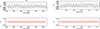 |
Fig. 11. Same as Fig. 10 but for TESS Sector 29. |
| In the text | |
|
Fig. 12. Phased lightcurves of residuals in TESS S2 data after removing the frequencies to the 4σ limit (S/N = 5.0). The period is 2.46 days, the epoch is BJD 2457000.0. Upper panel: points between 2458354.115 and 2458369.746. Lower panel: points between 2458354.747 and 2458381.519. |
| In the text | |
|
Fig. 13. Step-by-step analysis of the CHEOPS data processed with PIPE and removing the frequencies identified in the CHEOPS data one by one. The top panel depicts the three CHEOPS visits together, while the three bottom panels each represent the isolated visits. |
| In the text | |
Current usage metrics show cumulative count of Article Views (full-text article views including HTML views, PDF and ePub downloads, according to the available data) and Abstracts Views on Vision4Press platform.
Data correspond to usage on the plateform after 2015. The current usage metrics is available 48-96 hours after online publication and is updated daily on week days.
Initial download of the metrics may take a while.