| Issue |
A&A
Volume 676, August 2023
|
|
|---|---|---|
| Article Number | A136 | |
| Number of page(s) | 25 | |
| Section | Stellar atmospheres | |
| DOI | https://doi.org/10.1051/0004-6361/202346062 | |
| Published online | 23 August 2023 | |
Spectral energy distributions of classical Cepheids in the Magellanic Clouds★,★★
1
Koninklijke Sterrenwacht van België,
Ringlaan 3,
1180
Brussels,
Belgium
e-mail: martin.groenewegen@oma.be
2
Leiden Observatory, Leiden University,
PO Box 9513,
2300
RA Leiden,
The Netherlands
Received:
2
February
2023
Accepted:
4
July
2023
In this study, we constructed spectral energy distributions (SEDs) for a sample of 142 Large Magellanic Cloud (LMC) and 77 Small Magellanic Cloud (SMC) fundamental-mode classical Cepheids (CCs) using photometric data from the literature. When possible, the data were taken to be representative of mean light or averaged over the light curve. The sample was built from stars that either have a metallicity determination from high-resolution spectroscopy or have been used in Baade-Wesselink types of analyses, or have a radial velocity curve published in Gaia DR3 or have Walraven photometry, or have their light- and radial-velocity curves modelled by pulsation codes. The SEDs were fitted with stellar photosphere models to derive the best-fitting luminosity and effective temperature. Distance and reddening were taken from the literature. Only one star with a significant infrared (IR) excess was found in the LMC and none in the SMC. IR excess in MW CCs is not uncommon suggesting that IR excess may be more prominent in MW cepheids than in the Magellanic Clouds. The stars were plotted in a Hertzsprung-Russell diagram (HRD) and compared to evolutionary tracks for CCs and to theoretical instability strips. For the large majority of stars, the position in the HRD is consistent with the instability strip. Period-luminosity (PL) and period-radius relations were derived and compared to these relations in the MW. For a fixed slope, the zero point of the bolometric PL relation does not depend on metallicity, contrary to recent findings of a significant metallicity term when considering the PL relation in different photometric bands. The mass-luminosity (ML) relation is derived and it points to an over luminosity of about +0.3 dex with respect to a canonical ML relation. The most intriguing result concerns the flux-weighted gravity (FWG, a quantity derived from gravity and effective temperature) and its relation to period and luminosity. Both relations agree with theory, with the results for the MW and with the independent estimates from the six known LMC eclipsing binaries that contain CCs. However, the FWG (as determined from dedicated high-resolution spectroscopy for the sample) is too low by about 0.8 dex in 90% of the cases. Recent works on time-series data on 20 CCs in the MW were analysed finding a similar (but less extreme) offset in gravity and the FWG. Most importantly, other time-series data on the same 20 CCs are in full agreement with the FWG-period relation. The observed time-series of spectroscopic data and from a two-dimensional hydrodynamical cepheid model was used to investigate the so-called effective gravity, that is, the gravity corrected for a dynamical term related to the time derivative of the radial velocity. There is a reasonable good correspondence between the predicted effective gravity and the observed gravity as a function of pulsation phase, which would potentially allow for an independent estimate of the projection factor, but the dynamical term is too small to explain the overall difference between the observed (flux-weighted) gravity and the (flux-weighted) gravity derived from the SED modelling and stellar mass estimates.
Key words: stars: distances / stars: fundamental parameters / stars: variables: Cepheids
Full Tables 1, A.1, A.2, and B.1 are only available at the CDS via anonymous ftp to cdsarc.cds.unistra.fr (130.79.128.5) or via https://cdsarc.cds.unistra.fr/viz-bin/cat/J/A+A/676/A136.
The FITS to the SEDs are available at https://doi.org/10.5281/zenodo.8032168.
© The Authors 2023
 Open Access article, published by EDP Sciences, under the terms of the Creative Commons Attribution License (https://creativecommons.org/licenses/by/4.0), which permits unrestricted use, distribution, and reproduction in any medium, provided the original work is properly cited.
This article is published in open access under the Subscribe to Open model. Subscribe to A&A to support open access publication.
1 Introduction
Classical Cepheids (CCs) serve as an important standard candle because they are bright and provide a link between the distance scale in the nearby Universe and that further out, via galaxies that contain both Cepheids and SNIa (see Riess et al. 2022 for a determination of the Hubble constant to 1.0 km s−1 precision). Typically, the period-luminosity (PL) relations of CCs that are at the core of the distance determinations are derived, namely: the photometric filters (V, I, K) or combination of filters that are designed to be independent of reddening, the so-called Wesenheit functions (Madore 1982); for example, using combinations of (V, I), (J, K) or the combination used by the SH0ES team (F555W, F814W, and F160W HST filters, see Riess et al. 2022).
On the other hand, the bolometric magnitude or luminosity is a fundamental quantity of CCs as well as stars in general, as it is the output of stellar evolution models and the input to CC pulsation models. In Groenewegen (2020a, hereafter G20), the spectral energy distributions (SEDs) of 477 Galactic CCs were constructed and fitted with model atmospheres (and a dust component when required). For an adopted distance and reddening these fits resulted in a best-fitting bolometric luminosity (L) and the photometrically derived effective temperature (Teff). This allowed for the derivation of period-radius (PR) and PL relations, the construction of the Hertzsprung-Russell diagram (HRD), and a comparison to theoretical instability strips (ISs). The position of most stars in the HRD was consistent with theoretical predictions. Outliers were often associated with sources where the spectroscopically and photometrically determined effective temperatures differed, or in cases where the sources exhibit a high degree of reddening with large uncertainties as well.
This sample was further studied in Groenewegen (2020b), where the relation between bolometric absolute magnitude and the flux-weighted gravity (FWG), defined as log ɡF = log ɡ – 4 • log (Teff/104) (Kudritzki et al. 2003), was investigated: the so-called flux-weighted gravity-luminosity relation (FWGLR). The tight correlation between ɡF and luminosity was first demonstrated by Kudritzki et al. (2003, 2008) for blue supergiants (BSGs) and was later used for extra galactic distance determinations in Kudritzki et al. (2016). Anderson et al. (2016) then demonstrated that theoretical pulsation models for CCs also followed a tight FWGLR, one that is, in fact, tighter than the PL relation, finding that there was a good correspondence between observed ɡF and period for a sample of CCs. Groenewegen (2020b) presented the currently best observationally determined FWGLR for Milky Way (MW) CCs, based on the luminosities derived in Groenewegen (2020a) and gravity and effective temperatures from the literature.
In Groenewegen (2020a) the adopted distances were based as much as possible on Gaia parallax data (from DR2 in that case). However, we need to correct the catalogued parallaxes for the parallax zero-point offset (PZPO). In GDR2, this value was −0.029 mas for quasars (Lindegren et al. 2018) and for CCs −0.046 ± 0.013 (Riess et al. 2018) or −0.049 ± 0.018 mas (Groenewegen 2018, hereafter G18), and was also a limiting factor in improving upon the local distance scale. In GEDR3 the Gaia team provided a Python script to the community (Lindegren et al. 2021, hereafter L21), which Riess et al. (2021) applied to a sample of 75 CCs in the MW, concluding that a counter correction of −14 ± 6 µas is required. The advantage of using the Magellanic Clouds (MCs) is that accurate and independently derived mean distances are available based on the analysis of samples of eclipsing binaries (Pietrzyński et al. 2019; Graczyk et al. 2020).
The present paper performs a study similar to Groenewegen (2020a) and Groenewegen (2020b) for a sample of CCs in the Small (SMC) and Large (LMC) Magellanic Clouds. The paper is structured as follows. In Sect. 2, the sample of 219 MC CCs is introduced, while Sect. 3 introduces the photometry that is used, the distances used, how the stellar mass is estimated and how the modelling of the SED is done. Section 4 offers a discussion of key results, in particular, the location of the CCs in the Hertzsprung-Russell diagram, the presence of any infrared excess, the period-radius and period-luminosity relations, the mass-luminosity relation, and the relation between the FWG and period and luminosity. A brief discussion and summary is given in Sect. 5.
2 Sample
In this paper, we study a sample of 142 LMC and 77 SMC CCs. Although this is a small subset of the about 4700 LMC and 4900 SMC CCs known in the MCs (see e.g. Ripepi et al. 2017, Ripepi et al. 2022), the stars in this sample are of special interest as they have been studied in other respects. Specifically, the sample is composed of: a) 89 LMC CCs for which Romaniello et al. (2022) derived iron and oxygen abundances (as well as effective temperatures and gravities) from high-resolution (HR) spectroscopy. This sample is composed of 68 CCs used to define the PL-relation in the LMC in the SH0ES program (Riess et al. 2019) and 21 for which archival spectra, first presented in Romaniello et al. (2008), were re-analysed; b) 14 SMC CCs for which Romaniello et al. (2008) performed an abundance analysis. We note that for the LMC CCs in overlap Romaniello et al. (2022) derived an iron abundance that was (on average) 0.1 dex smaller compared to Romaniello et al. (2008); c) 7 CCs in the LMC cluster NGC 1866 (Molinaro et al. 2012; Lemasle et al. 2017) and four field SMC objects (Lemasle et al. 2017) with iron abundances from HR spectroscopy; d) CCs for which a Baade-Wesselink analysis has been carried out, in particular: 36 LMC and five SMC stars considered in Storm et al. (2011), and the almost identical sample of 36 LMC and six SMC stars analysed in Groenewegen (2013). Similarly, 27 LMC and eight SMC stars that have been analysed with the SPIPS code (Mérand et al. 2015) in Gallenne et al. (2017) to derive the pulsation (p) factor; e) CCs for which light-curves (and sometimes radial-velocity curves) have been fitted with theoretical pulsation models. In such a modelling (Marconi et al. 2013) the stellar mass, luminosity, and (mean) effective temperature are derived by fitting the light-curves (typical V, I, and K). The apparent distance moduli (DM) are derived from which the true DM and reddening are found. If RV curves are fitted, the projection-factor (p-factor) is also derived. Here, we consider the 11 LMC and 9 SMC fundamental-mode (FM) CCs studied in Ragosta et al. (2019) and Marconi et al. (2017), respectively; f) CCs with (previously unpublished) photometry in the Walraven (Walraven & Walraven 1960) system. This system is very usefull in constraining effective temperature and reddening as the photometric bands extend into the blue. van Genderen (1983) published VBLUW photometry for 21 SMC and 20 LMC CCs using data taken between 1971 and 1978 in South Africa (also see van Genderen 1981; Pel et al. 1981; van Genderen & Nitihardjo 1989). However, data collection continued from 1979 onwards from Chile and in Appendix A we report on these observations.
Furthermore, we have g) CCs in the MCs with RV curves published in Gaia DR3 (Ripepi et al. 2023; Gaia Collaboration 2023, Gaia Collaboration 2016); h) SMC FM CCs for which UVES spectra and in part HST photometry will be obtained in the near future1.
There are stars contained in the overlap between the different subsamples and the final sample consists of 142 LMC and 77 SMC CCs, all of which are FM pulsators. The basic parameters of the stars are compiled in Table 1.
3 Photometry, distance, masses, and modelling
3.1 Photometry
The SEDs were constructed using photometry retrieved mainly (but not exclusively) via the VizieR web-interface2. Data were considered (in increasing wavelength) in the UV from GALEX (Bianchi et al. 2017), in the optical from a variety of sources, namely, OGLE (B, V, I) photometry from Udalski et al. (1998) (SMC) and Udalski et al. (2000) (LMC), (V, I) photometry from the OGLE Shallow Survey in the LMC (Ulaczyk et al. 2012, 2013), and OGLE-IV data for both Clouds Soszyński et al. (2017), Gaia Bp, G, and Rp photometry from DR3 (Gaia Collaboration 2023), (B, R) photometry from the EROS survey in the LMC (Kim et al. 2014), (u,υ,g,r,i,z) data from Skymapper DR2 (Onken et al. 2019), (B, V, R, I) photometry for LMC CCs from Sebo et al. (2002), (U,B,V) photometry from Madore (1975), Eggen (1977), and Martin & Warren (1979), Walraven (VBLUW) photometrey (see Appendix A), (U, B, V, I, K) for CCs in NGC 1866 from Musella et al. (2016), HST F555W, F814W, and F160W photometry from Riess et al. (2019) for LMC Cepheids, and further to the near- and mid-infrared, (Y, J, K) photometry from the VMC survey (Cioni et al. 2011) for the SMC (Ripepi et al. 2016) and LMC (Ripepi et al. 2022), and from the public DR6 for a few remaining stars, (J, H, K) photometry for LMC CCs from Persson et al. (2004) and Macri et al. (2015), Akari photometry for the SMC (Ita et al. 2010) and LMC (Kato et al. 2012). We note that for the S7, S11, and L15 filters, only errors in the magnitudes of <0.15, <0.20, and <0.20 mag, respectively, were accepted. Then, we also used AllWISE photometry (Cutri & et al. 2014; in the W3 and W4 filters only errors in the magnitudes of <0.30, and <0.25 mag, respectively, were accepted), Spitzer IRAC photometry from Chown et al. (2021; mean magnitudes from template fitting in the 3.6 and 4.5 µm bands) and from VizieR catalogue II/305/catalog in the 5.8 and 8.5 µm bands. Finally, we used MIPS photometry at 24 µm available from the IRSA3. No MIPS data at 70 µm were available.
The number of available photometric data points for the LMC CCs ranges from 16 to 39, with a median of 30, and for the SMC objects from 15 to 29, with a median of 20 photometric points. The data contain single-epoch observations (typically from GALEX and Akari) but whenever possible values at mean light were taken or multiple datapoints were averaged.
Sample of stars (selected entries).
3.2 Distance and geometric correction
The mean distance to the LMC is adopted to be dLMC = 49.59 ± 0.09 (stat) ± 0.54 (syst) kpc (Pietrzyński et al. 2019), and to the SMC of dSMC = 62.44 ± 0.47 (stat.) ± 0.81 (syst.) kpc (Graczyk et al. 2020), based, in both cases, on the analysis of samples of eclipsing binaries. The depth effect in the SMC is considerable, for example Ripepi et al. (2017), but all SMC sources have been adopted to be at the mean distance. For the LMC the first order approximation of an inclined disk is adopted to compute the geometric correction and the procedure in Riess et al. (2019) is followed, taking the inclination and position angle of the line of nodes of the disk from Pietrzyński et al. (2019) and the LMC center-of-mass coordinates from van der Marel & Kallivayalil (2014). The adopted distances are listed in Col. 4 in Table 1.
3.3 Stellar masses
An estimate for the stellar mass is required when computing the stellar gravity, with the stellar radius available from the best-fitting luminosity and effective temperature combination, as detailed below. Several methods have been employed to this end. First, the period-luminosity-mass-effective temperature-metallicity relation derived in Groenewegen & Jurkovic (2017) based on the models of Bono et al. (2000b).
Alternatively, and in a similar way, such a relation was derived here based on the models of Anderson et al. (2016). That paper gives, for a given mass, metallicity and rotational speed – the period, luminosity, and effective temperature at the start and end of the IS, and for different crossings of the IS a star may undergo. As the first-crossing is very short compared to the other crossings these models were not considered. An initial fit showed that the metallicity term is not significant. The best linear fit for average rotation, all metallicities, and the second and third crossing models for FM pulsators is:
 (1)
(1)
Based on the model fitting of LMC Cepheid light curves Ragosta et al. (2019) presented a period-mass-radius relation of
 (2)
(2)
with a dispersion of only 0.005 dex. This relation will be applied to the SMC ones as well.
Pilecki et al. (2018) analysed the light- and radial-velocity curves of the six known cepheid containing eclipsing binaries (containing seven Cepheids, including one type-II cepheid (T2C), all in the LMC). For convenience, the stellar parameters they derived for the Cepheids are compiled in Table 2, as they appear in several plots. Pilecki et al. (2018) derived the following period-mass-radius relation
 (3)
(3)
with a dispersion of 0.037 dex. This relation will be applied to the SMC ones as well. The mass range on which this relation is based is smaller than that of the other relations.
Marconi et al. (2020) used nonlinear convective pulsation models to link period and mass to a Wesenheit index based on Gaia magnitudes. For a mixing length parameter of 1.7 and FM pulsators Marconi et al. (2020) give:
 (4)
(4)
with a dispersion of 0.058 mag, and where WG = G – 1.90 • (Bp – Rp) (Ripepi et al. 2019) and DM is the distance modulus. The pulsation models were calculated at solar metallicity but will be used for the MC CCs.
The mass estimates from these five methods are listed in Table B.1. The adopted mass is the median among the five estimates, and is listed in Table B.1 and in Col. 12 in Table 1. To estimate the error bar, the error in the mass estimate of the median value is added in quadrature to the median-absolute-deviation times 1.48 (to get the equivalent of one sigma in a Gaussian distribution) among the five estimates.
The different estimates are in good agreement in most cases, except for some of the longest period Cepheids where some individual estimates give unrealistically low masses, leading to the median value becoming also unrealistically low. These values are set between parenthesis and have not been used in the analysis. The origin of the discrepancy is probably related to the fact that the different mass-estimate formalisms are not derived from such long-period Cepheids.
3.4 Modelling
The SEDs are fitted with the code More of DUSTY (MoD, Groenewegen 2012)4 which uses a slightly updated and modified version of the DUSTY dust radiative transfer (RT) code (Ivezić et al. 1999) as a subroutine within a minimisation code. As we are not interested in any dust component the dust optical depth is initially set to zero. In that case, the input to the model are the distance, reddening, and a model atmosphere. The few cases where an infrared (IR) excess may be present are discussed in Sect. 4.3.
The model atmosphere fluxes are reddened to be compared to the observations. The reddening map of Skowron et al. (2021) for the MCs is adopted and the E(V–I) value in the map closest to the source is taken. The visual extinction is then assumed to be Av = 3.1 • E(V–I)/1.318, and is listed in Col. 5 in Table 1.
MARCS model atmospheres are used as input (Gustafsson et al. 2008) for log ɡ = 1.5 and metallicity −0.50 and −0.75 dex for the LMC and SMC stars, respectively. The model grid is available at 250 K intervals for the effective temperature range of interest, and adjacent model atmospheres are used to interpolate models at 125 K intervals, which better reflects the accuracy in Teff that can be achieved. For every model atmosphere (that is, Teff) a best-fitting luminosity (with its (internal) error bar, based on the covariance matrix) is derived with the corresponding reduced χ2 ( ) of the fit. The model with the lowest
  then gives the best-fitting effective temperature. Considering models within a certain range above this minimum
  then gives the estimated error in the effective temperature and luminosity. For the luminosity, this error is added in quadrature to the internal error in luminosity.
The best fitting effective temperature and luminosity with error bar are listed in Cols. 9 and 10, and the resulting radius in Col. 11 of Table 1. Combined with the mass this gives the gravity (Col. 13), and gravity combined with Teff the FWG (Col. 14).
Stellar parameters of the Cepheid in known LMC EBs (from Pilecki et al. 2018).
4 Results and discussion
4.1 General
Figures 1 and D.1 present the four best, respectively, the four poorest fits to the SEDs (according to the  ), respectively, with the residual (model minus observations) in the bottom part of each panel5. In the model fitting procedure photometric outliers were excluded in the following way. The rms in the residuals was determined and added in quadrature to the photometric error bar for each data point. If the absolute difference between model and observations was larger than 4σ the point is flagged and plotted with an error bar of 3.0 mag to still identify it but to have no influence on the fitting.
The fits are quite acceptable. In the poorest fits the scatter among the various photometric points is larger overall. In the case of SMC0417 and SMC0921 this leads to the result that the most visually discrepant points (the VMC JHK points) are not marked as 4σ outliers and that therefore the reduced χ2 is large.
A limitation of our procedure is that time variability of the photometry is not taken into account. Values at mean light have been considered whenever possible, but the SEDs also contain single-epoch data. Pulsation amplitudes decrease with wavelength so the effect should not play a major role in the mid and far-IR and in the NIR where the SEDs peak mean-light magnitudes are typically available. The construction of the SED at mean light also ignores possible phase shifts between photometric bands.
We have compared our results to the fully independent modelling by Gallenne et al. (2017) using the SPIPS code (Mérand et al. 2015) for 35 stars in overlap. The SPIPS code takes light curves as input and therefore considers the time variability. It is also independent in the sense that it fits ATLAS9 model atmospheres (Castelli & Kurucz 2003).
Figure 2 compares the result and the agreement is excellent. The rms in the residuals is about 160 K in Teff and 0.05 dex in log L. The effective temperature plot suggest that the errors in effective temperature may have been overestimated by about ~ 40% in both studies.
4.2 Hertzsprung-Russell diagram
Figure 3 shows the HRD together with sets of evolutionary tracks and ISs. Objects from the sample are plotted as black (LMC) and red (SMC) open squares, respectively. Stars located outside the bulk of objects are plotted with error bars, and some are labelled as well. Blue symbols with error bars indicate the six CCs in EBs (three FM as filled squares, three FO as filled triangles; see Table 2).
Two sets of ISs from De Somma et al. (2021) (at brighter magnitudes) and from Pilecki et al. (2018) (at fainter magnitudes) are plotted. The near horizontal green lines indicate the evolutionary tracks for Z = 0.006 and average initial rotation rate ωini = 0.5 from Anderson et al. (2016). Increasing in luminosity are tracks for initial mass (number of the crossing through the IS): 4 (1), 5 (1), 7 (1), 7 (2), 7 (3), 9 (1), 9 (2), 9 (3), 12 (1), and 15 M⊙ (1). The density of stars in the HRD is qualitatively consistent with the fact that the first crossing is much faster than the second and third crossings.
There are only two clear outliers, LMC1940 and LMC1945, and their position in the HRD remains unexplained. The former object has the fourth poorest fit, but the  of the fit of LMC1945 is not extremely poor. LMC1940 and LMC1945 have large Gaia astrometric_gof_al (GoF) parameters of about 12 and 9.9, respectively (and RUWE values of 1.56 and 1.43, respectively), which may hint to binarity. However, 38 stars in the sample have a larger GoF than 9.9 and are not outliers in the HRD diagram. A cautionary note is that the SED fitting assumes the stars to be single. Contamination of the photometric points by a companion will have an influence on the results of the fitting procedure. No spectroscopic temperature determinations is available for LMC1945. For LMC1940 there is a value of 4909 ± 126 K determined from APOGEE data (Sprague et al. 2022). A model with 4875 K (the closest in the available grid) was run to find that the luminosity is about 13% less than in the best-fitting model. This temperature and luminosity would put the star closer to the red edge of the IS, but still too cool and overly under-luminous, compared to expectations.
The location of the known CCs in EBs in noteworthy. Five of them are clearly hotter than expected from the IS by De Somma et al. (2021) but are consistent with the IS as calculated by Pilecki et al. (2018). It is noted that the effective temperatures in Pilecki et al. (2018) have not been derived from the available (disentangled) spectra that these authors used to obtain the radial velocities, but from effective temperature–colour relations using the V – I (sometimes V – K) colour of the two components, as derived from the modelling of the light curve. This may have possibly introduced a systematic effect. If the temperatures derived in this way would end up being too high, the luminosities would also be too large, as indeed inferred from the PL-relation (see below).
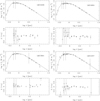 |
Fig. 1 Four best-fitting models. The upper panels: Observations (with error bars) and the model. The lower panels: Residuals. Outliers that have been clipped are plotted with an (arbitrary) error bar of 3.0 mag. |
Effect of dust on the colours of CCs.
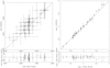 |
Fig. 2 Comparison of effective temperature and luminosity between the present work and the 27 LMC (filled circles) and 8 SMC (open circles) stars in overlap. The bottom panels show the residuals. |
4.3 Infrared excess
The default assumption in the modelling has been that there is no IR excess and the SEDs can be modelled by a stellar atmosphere. However, near- and mid-IR excess is known to exist in Galactic CCs, for example, direct interferometric observations in the optical or NIR (e.g. Kervella et al. 2006; Mérand et al. 2006; Gallenne et al. 2012; Nardetto et al. 2016), modelling with the SPIPS code (e.g. Breitfelder et al. 2016; Trahin 2019; Trahin et al. 2021, and Gallenne et al. 2017 for the LMC) and was also found in modelling the SEDs of Galactic CCs (Gallenne et al. 2013, G20).
Visual inspection of the SEDs showed five cases where an IR excess could explain the shape of the SEDs6. Following G20, models were run for these five stars including a dust component and additionally fitting for the dust temperature at the inner radius and the dust optical depth under the assumption of spherical symmetry. Following G20, a mixture of 3% silicate, 3% aluminium oxide and 94% iron dust was adopted. The analysis of the MW CCs in G20 with available mid-IR spectra showed that these are near featureless requiring a large fraction of featureless iron dust, although the nature of the excess is in fact unclear. The results of the fitting are listed in Table 3 that include the magnitudes in various filters for the best-fitting model excluding and including a dust component.
Only the model for LMC0619 is convincing with an excess in four to five filters (see Fig. 4) and an SED comparable in shape to the SEDs of the MW CCs with IR excess. In the other four cases, the temperature at the inner radius is very low and based on two filters only (see Fig. D.2). Also, the reduction in the Bayesian information criteria (BIC) is small.
Interestingly, the best-fitting model with dust predicts fainter magnitudes for LMC0619. For fixed effective temperature and luminosity and for optically thin cases, one expects some absorption in the optical and emission in the IR. However, in the fitting the effective temperature and luminosity were allowed to vary, and the best-fitting luminosity is lower when including dust. The difference in the Wesenheit filters is around 0.15 mag, which is significant.
Only one of 142 CCs in the LMC, and 0/77 in the SMC has a convincing IR excess. Coincidence or not, LMC0619 has the longest period of the LMC objects (133 days) and one of the highest luminosities. In the MW, IR excess is quite common (see references at the beginning of the section) and G20 lists 16/347 stars as having an IR excess, also based on SED fitting. It appears that the presence of IR excess is more common in the MW than in LMC and SMC CCs For comparison, one of the MW stars with IR excess from G20, LS Pup, was refitted and the results are included in Table 3 and Fig. D.2. A definite conclusion would require a more in debt study beyond the scope of the present paper, as one would have to consider the impact of the bias due to the fact that for MW CCs more data is available (in some cases even mid-IR spectra) especially at longer wavelengths. The SED modelling is therefore more likely to find an IR excess in MW stars than in the MCs.
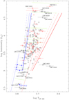 |
Fig. 3 Hertzsprung-Russell diagram. Black and red open squares indicate LMC and SMC CCs from the sample, respectively. Stars located outside the bulk of objects are plotted with error bars, and some are labelled as well. Blue symbols with error bars indicate the six CCs in EBs (three FM as filled squares, three FO as filled triangles, see Table 2). Blue and red lines indicate the blue and red edge of the IS. In the upper part (brighter than log L = 3), the results from De Somma et al. (2021) are plotted. The thinner solid and dot-dashed line are for Z = 0.008 and Z = 0.004 models, respectively, for their type A mass-luminosity relation. The tick line is for Z = 0.008 for their type-B mass-luminosity relation. In the lower part (fainter than log L = 3.5), the results from Pilecki et al. (2018) are plotted for FM (solid lines) and FO (dotted lines) model. Green lines indicate evolutionary models from Anderson et al. (2016). See the main text for details. |
4.4 Period-luminosity relations
Figure 5 shows the PL relation. A fit to 141 LMC objects (removing one object through 3σ clipping) is:
 (5)
(5)
with an rms of 0.20 mag. A fit to 77 SMC objects (removing zero outliers) is:
 (6)
(6)
with an rms of 0.25 mag.
LMC1940 is an outlier in the HRD, but also in the PL-relation. Its period would suggest Mbol ≈ −4.0, or log L ≈ 3.5. In the HRD, this would move the star up but it would still be an outlier and too cool for its expected position. Although it is underluminous for a CC LMC1940 is too luminous to be a Type-II cepheid (T2C), as indicated by the PL-relation for T2Cs from Groenewegen (2020a). We also note that the CCs in EBs are slightly brighter than the mean relation.
In G20 the slope and the zero point (ZP) based on 380 Galactic CCs were derived to be −2.95 ± 0.09 and −0.98 ± 0.07 (rms of 0.40 mag), respectively. The slopes derived for the three galaxies agree to within the error bar. Fixing the slope to the most precise one of that in the LMC (−2.96), ZPs of −4.057 ± 0.002 and −4.046 ± 0.004 are found for LMC and SMC at log P = 1, respectively.
The bolometric PL relation to the Galactic Cepheids presented in G20 did not select based on metallicity. Figure D.3 shows the distribution in [Fe/H] of the stars that went into that fitting. The 5–95% range is from −0.31 to +0.29 dex, with a median of +0.06. Selecting stars in the range 0.0 ≤ [Fe/H] <+0.2 to better have a sample of near solar metallicity leads to a median of +0.09 (with 0.06 dex dispersion7) and a PL-relation of
 (7)
(7)
with an rms of 0.35 mag using 191 stars, and a ZP of −4.041 ± 0.002 at 10 days for a fixed slope of −2.96.
Figure 6 shows the ZP at 10 days plotted against metallicity. The metallicity for the MW is the one just derived, for the LMC −0.409 dex with dispersion of 0.076 (Romaniello et al. 2022) is adopted and for the SMC, a value of −0.75 dex with dispersion of 0.08 (Romaniello et al. 2008) is assumed. A least-squares fit taking into account the error bars in both axes gives
![$ {\rm{ZP@10d}}\,{\rm{ = }}\,\left( { - 4.0451 \pm 0.0036} \right) + \left( { + 0.0082 \pm 0.0075} \right) \cdot \left[ {{{{\rm{Fe}}} \mathord{\left/ {\vphantom {{{\rm{Fe}}} {\rm{H}}}} \right. \kern-\nulldelimiterspace} {\rm{H}}}} \right] $](/articles/aa/full_html/2023/08/aa46062-23/aa46062-23-eq14.png) (8)
(8)
Using slightly different values for the LMC, for example, −0.35 ± 0.09 dex for BSGs (Urbaneja et al. 2017), or −0.62 ± 0.14 dex for SMC cluster giants (Trundle et al. 2007, as quoted in Romaniello et al. 2008) all lead to slight positive but insignificant slopes. A constant value of −4.049 mag with dispersion 0.008 mag would fit the ZPs of all three galaxies.
The result that the bolometric PL relation does not seem to depend on metallicity is in contrast with the most recent results of Breuval et al. (2022) that derive the metallicity term in various filters from Gaia Bp band to IRAC 4.5 µm and find little dependence on wavelength and an average of γ = −0.29 mag dex−1. Our results indicate that the LMC Cepheids are indeed brighter than the SMC ones (this is so when γ is negative, and fitting only the SMC and LMC data points gives γ = −0.04) but it would imply that the ZP for the MW Cepheids is too faint by (−0.75 − +0.08) • −0.29 ≈ 0.24 mag. Further study is required, especially on the MW sample, and parallaxes from Gaia DR4 will be crucial in this regard. Additionally, the difference between the bolometric magnitude and the magnitude in any photometric band involves a bolometric correction that should depend on wavelength and makes a direct comparison of the γ terms less evident.
 |
Fig. 4 Best-fitting model without dust (left side) and with dust (right side) for the star with the most convincing presence of an IR excess. In the model without dust, the long-wavelength points are considered outliers. |
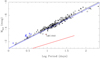 |
Fig. 5 Period-Mbol relation. Error bars in Mbol are plotted but are typically smaller than the symbol size. LMC objects are plotted as open squares, SMC objects are filled squares. Blue symbols indicate the six CCs in EBs. One outlier is marked by a red cross and is identified. The black line indicates the best fit (excluding the outlier) to the complete MC sample. Fits to the LMC and SMC stars separately are given in the text. The blue line gives the PL relation for MW CCs from G20, while the red line gives the recommended solution for T2C (Groenewegen 2020a). |
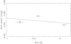 |
Fig. 6 Zero point at 10 days of the PL-relation for SMC, LMC, and MW. The line is a linear fit with a slope (0.0082 ± 0.0076) mag dex−1 which is not significant. |
4.5 Period-radius relation
Figure 7 shows the PR relation. The relation for the LMC is:
 (9)
(9)
with an rms of 0.017 dex and using 138 stars (removing 4 outliers), and then for the SMC
 (10)
(10)
with an rms of 0.027 dex and using 76 stars (removing 1 outlier). Figure 7 also shows the PR relation for MW CCs from G20. The slope derived there was 0.721 ± 0.013 with a ZP of 1.083 ± 0.012. Refitting the data in G20 restricting the metallicity to 0.0 ≤ [Fe/H] <+0.2 gives:
 (11)
(11)
with an rms of 0.069 dex and using 190 stars. The slopes are consistent with each other and at P = 10 d the radii in MW, LMC, and SMC CCs are identical to within the error bars.
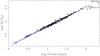 |
Fig. 7 Period-radius relation. LMC objects are plotted as open squares, SMC objects are filled squares. Blue symbols indicate the six CCs in EBs. Outliers removed from the fit are marked by a red cross and some are identified. The black line indicates the best fit (excluding the outliers) to the complete MC sample. Fits to the LMC and SMC stars separately are given in the text. The blue line gives the PR relation for MW CCs from G20. |
4.6 The mass-luminosity relation
Figure 8 shows the relation between mass and luminosity. The best fit is:
 (12)
(12)
based on 208 stars and an rms of 0.12 dex, and lies approximately 0.3 dex above the canonical ML relation from Bono et al. (2000a) for Helium abundance Y = 0.255 and metallicity Z = 0.008. A few stars scatter clearly above the relation. The few stars that scatter below the best-fit relation are consistent with the canonical ML relation. The best-fit relation is the intermediate between the case B (+0.2 dex w.r.t. the canonical relation) and case C (+0.4 dex) ML relations adopted in Marconi et al. (2020).
4.7 Comparing stellar parameters
The determination of the photometric effective temperature allows one to compare it to the spectroscopic temperature determined in the literature. In addition, via the derived luminosity, and estimated mass, it is possible to compare the gravity to that derived by spectroscopy. The values for the spectroscopic effective temperature and gravity come from the papers that contribute a large fraction of the stars in the sample (Romaniello et al. 2008, 2022; Lemasle et al. 2017). In addition, spectroscopicly derived parameters from the APOGEE survey have been considered (Sprague et al. 2022), as well as the values derived from the LC fitting in Ragosta et al. (2019) and Marconi et al. (2017). The adopted values for temperature and gravity are listed in Cols. 6 and 7 of Table 1. When data from multiple references were available the order of preferences was Romaniello et al. (2022, 2008), Lemasle et al. (2017), Sprague et al. (2022), and Marconi et al. (2017) or Ragosta et al. (2019). Results from GDR3 were not considered in the end. The results from the GSP_Spec analysis (Recio-Blanco et al. 2023) were inspected but only one, respectively two, had an entry from the so called Matisse-Gauguin and ANN pipeline when selecting ’000000’ for the first six values in the flags_gspspec and flags_gspspec_ann flags.
Figure 9 shows the comparison of the photometric and literature temperatures. On average the spectroscopic temperatures seem to be slightly larger, although there is large scatter. The median offset is +91 ± 330 K. The effective temperature changes over the pulsation cycle so an exact agreement is in fact not expected. The spectra taken from the works dedicated to determining the metallicity (and Teff and log ɡ in the process, Romaniello et al. 2008, 2022; Lemasle et al. 2017) of CCs typically try to avoid the phases where shocks play a role the objects. On the other hand the APOGEE data were taken at random phases while the photometric temperatures was derived from the SED that was constructed to be as much as representative of mean light as possible.
Figure 10 shows the same for the log ɡ values determined in the literature. The overall median offset is −0.70 ± 0.36 dex, but it strongly depends on the source. The log ɡ values derived from the pulsation models are in very good agreement with the values determined in the present paper, the values from APOGEE are larger (median offset +0.58 ± 0.46 dex), while those derived from dedicated HR spectroscopy are significantly smaller (median offset −0.80 ± 0.21). A similar plot for the FWG is shown in the Appendix (Fig. D.4).
The differences between the spectroscopic and photometric effective temperature are relatively small, but the spectroscopically determined gravity (and the FWG) from Romaniello et al. (2008, 2022) and Lemasle et al. (2017) are systematically and significantly smaller than that derived from L, Teff, and stellar mass. Like the effective temperature the gravity also changes over the pulsation cycle. There is a change in radius, but there is also a dynamical term. What is thus determined from HR spectroscopy is the effective gravity:
 (13)
(13)
where M is the mass of the CC, R(t) is the radius as a function of time (or pulsation phase), p is the projection factor (see Nardetto et al. 2004 and references therein) and Vr(t) is the radial velocity at the time t.
Recently, da Silva et al. (2022) presented time series of HR spectroscopy for 20 calibrating MW CCs and the analysis of these spectra in terms of radial velocities, metallicities, micro turbulent velocities, gravities and effective temperatures (see their Appendix B). This unique dataset also allows to study the effect of the effective gravity. The dynamical term  at each phase point ϕi was approximated as
  and a typical p factor of 1.25 was adopted.
The effective gravity is calculated as log ɡeff = 10log gmean + (dynamical term), where gmean is the weighted mean gravity over all available phase points (recalculated in the present paper and identical to the values in Table 6 of da Silva et al. 2022). This ignores the variation in radius with phase but this effect is smaller than the dynamical term (Appendix C). Figure 11 shows the result for δ Cep. The figure is ordered in such a way that the dynamical term appears below the RV curve and the calculated effective gravity appears below the observed gravity. Contrary to the convention in da Silva et al. (2022) phase 0 is taken at maximum light. Plots for some of the stars with the best phase coverage are shown in Appendix D (Figs. D.5–D.8). Overall there is reasonable to good correspondence between the effective gravity and the observed gravity, and the expected rise in gravity due to the dynamical terms occurs at the correct phase. The results show that if observations are taken at phases that avoid the sharp rise in radial velocity the effective temperature and gravity will be systematically lower than the average over the light curve. However, the effect should be a few 0.1 dex, and cannot explain the large difference between the spectroscopic and evolutionary gravity noted in Fig. 10. The behaviour of the effective gravity is also confirmed by a theoretical model, see Appendix C. It is beyond the scope of the present paper, but the analysis of time series data, as presented in da Silva et al. (2022), allows one to put constrains or derive the p-factor for individual stars, as the dynamical term is proportional to p and the effective gravity should match the observed gravity.
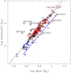 |
Fig. 8 Mass-luminosity relation. Objects in the LMC are plotted as black, those in the SMC as red open squares. Stars outside the bulk of objects are identified. Objects in blue are the known CCs and their companions in EBs. The blue line indicates the canonical ML relation from Bono et al. (2000a) for Y = 0.255 and Z = 0.008. For Z = 0.004 the line would be at higher luminosities by about 0.1 dex. The black line indicates a fit to the LMC stars minus the outliers (see Eq. (12)) and lies almost exactly +0.3 dex above the canonical ML relation. |
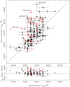 |
Fig. 9 Comparison between the effective temperatures determined from the SED fitting and in the literature. Objects in the LMC are plotted in black and objects in the SMC in red. The one-to-one line is indicated. Stars where the absolute difference is larger than 1000 K are identified. Objects from reference 1 and 2 (see the note to Table 1) are plotted as filled squares, from reference 3 as open squares, from reference 4 as filled triangles, from reference 5 as open triangles, and from reference 6 as filled circles. In the lower panel, the difference between literature and photometric temperature is plotted. |
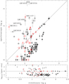 |
Fig. 10 Comparison between the log ɡ determined in the literature, and the evolutionary value as determined from L and Teff from the SED fitting and the stellar mass based on various methods (see Appendix B). The one-to-one line is indicated. Stars outside the bulk of objects are identified. Symbols as in Fig. 9. |
4.8 FWG-period and the FWGLR
Figure 12 shows the relation between the FWG and the pulsation period based on the analysis in the present paper as well as on the available HR observations for the sample and two identical samples of MW CCs. The best fit to the LMC objects is:
 (14)
(14)
with an rms of 0.057 dex, and is indistinguishable from the best fit to the SMC objects:
 (15)
(15)
with an rms of 0.062 dex. The preferred solution combines the SMC and LMC objects as follows:
 (16)
(16)
with an rms of 0.059 dex using 212 stars. This relation is in good agreement both with the theoretical prediction log ɡF = (−0.834 ± 0.011) log P + (3.402 ± 0.011), derived in Groenewegen (2020b) based on the models in Anderson et al. (2016) and the relation log ɡF = (−0.80 ± 0.03) log P + (3.43 ± 0.03) derived for MW CCs (Groenewegen 2020b).
Of interest are the location of all the coloured points in this plot. The blue points indicate the CCs and one T2C in EBs and these agree well with the observed relation. That some appear to be slightly above the relation could be related to an overestimate of the effective temperature, as argued before. The red circles indicate the objects from the sample where a FWG is available from HR spectroscopy. Almost all lie clearly above the relation, and those that do appear to be on a line parallel to the derived relation with on offset of about 0.8 dex (also see Fig. D.4). To investigate this further we again used the data from da Silva et al. (2022) on 20 calibrating MW CCs. These points are the light blue squares8. Except for the shortest period value (R TrA at P = 3.4 days), which agrees well with the mean relation all others form a sequence that lies above and is inclined to the mean relation. All these 20 CCs also have (in part multi-epoch) HR spectroscopy data that is analysed in Luck (2018), which was the main source of data used in our previous study on MW Cepheids (Groenewegen 2020b). These points are the green squares and those fit Eq. (16) very well. If we demand that the absolute difference between the observed FWG and that predicted by Eq. (16) is less than  with σFWG the observed error in the FWG than all 20 objects from Luck (2018) obey this relation for δ = 1.5. For this value of δ only 4 out of the same 20 objects obey this relation using the FWGs from da Silva et al. (2022) – and even these four stars all lie above the relation – and only 99 out of 104 stars using the FWGs as derived from HR spectroscopy in the MCs. It is beyond the scope of the present paper to investigate this further (see also the discussion and appendix in Groenewegen 2020b, where a similar effect was noticed). Nevertheless, Fig. D.9 shows the comparison between temperature, gravity, and the differential between Luck (2018) and da Silva et al. (2022) for the same 20 objects. Most interesting is the result that there is a correlation between the two data sets. When for an object Teff is larger in Luck (2018) then in da Silva et al. (2022), then also the gravity is larger.
Figure 13 shows the FWGLR. Using a least-squares fit taking into account errors in both axes gives the following fit to the LMC objects:
 (17)
(17)
with an rms of 0.16, and a fit to the SMC CCs of:
 (18)
(18)
with an rms of 0.12. The combined fit is the preferred solution and is expressed as:
 (19)
(19)
with an rms of 0.12 mag using 207 objects. Blue filled squares in the plot indicate the six EB CCs and their companions, the filled red square indicates the T2C in the LMC-T2CEP-098 system and the filled black square its companion. Except for the T2C itself, the CCs, and the companions agree very well with Eq. (19). Where there is overlap at small FWGs, there is also good agreement with the FWGLR derived for BSGs in the LMC (Urbaneja et al. 2017; Bresolin et al. 2022).
This demonstrates the power of the FWGLR as the BSGs have masses in the range 12–40 M⊙ (Fig. 5 in Urbaneja et al. 2017), while the Cepheids in the present sample have lower masses that are estimated to be in the range 2.8–13.5 M⊙ (median of about 6 M⊙). Using evolutionary tracks Kudritzki et al. (2020) demonstrated that, what they named an “extended,” FWGLR is expected over 17 magnitudes in Mbol (with a scatter of 0.17 mag below Mbol = −3.0 mag) and for masses in the range 0.8–40 M⊙, which they verfied using a sample of RGB stars with a typical mass of 1.1 M⊙.
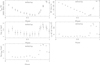 |
Fig. 11 Time series of effective temperature, radial velocity and gravity for δ Cep from da Silva et al. (2022). Calculated in the presented paper are the dynamical term and the effective gravity based on the mean gravity and the dynamical term. The ordinate for the effective gravity is set to that of the observed gravity. |
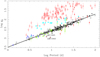 |
Fig. 12 FWG versus log P. Black points indicate the FWGs derived from L and Teff (from the SED fitting) and stellar mass in the present paper. Black open squares are LMC objects, filled squares indicate SMC objects. Blue symbols indicate the CCs (filled squares) and one T2C (filled triangle) in EB systems. The black line is a fit to the black points, minus the two marked outliers. The red circles indicate FWGs from HR spectroscopy (open circles indicate LMC, filled circles indicate SMC), Light blue filled squares indicate FWGs of 20 MC CCs from da Silva et al. (2022), while the green points indicate the FWGs for the same 20 objects from Luck (2018; open squares indicate that only one spectrum is available in Luck 2018, filled squares indicate that five or more spectra are available). |
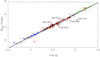 |
Fig. 13 FWGLR: LMC and SMC objects are identified by black and red open squares. To avoid cluttering the plot, representative error bars are plotted for the smallest and largest values of log ɡF only. Some outliers are marked, and stars excluded from the fit are marked by a red cross. Blue filled squares indicate the six EB CCs and their companions, the filled red square indicates the T2C in the LMC-T2CEP-098 system and the filled black square its companion. The black line gives the best fit to the objects (Eq. (16)). The green line at small FWGs is the fit to LMC BSGs (Urbaneja et al. 2017; Bresolin et al. 2022). |
5 Discussion and summary
This paper is a follow-up of G20 and Groenewegen (2020b), where the SEDs of 477 MW Cepheids were fitted. All stars had metallicities based on HR spectroscopy from the literature. Excluding non-CCs and overtone pulsators the PL, the PR and other relations were typically based on about 370 FM CCs. Some of the relations have been redetermined in the present paper using a restricted range in metallicity to have a sample of MW CCs with near solar metallicities and these relations are typically based on 190 CCs.
The present study covers 142 LMC and 77 SMC FM CCs. All known (FM) CCs in the MCs with metallicities based on HR spectroscopy are included and those constitute about half of the sample. Other CCs are included because they were studied otherwise (for example a Baade-Wesselink analyses was conducted) or may be of interest in future work (ongoing spectroscopic or HST observations). The advantage of the current sample compared to the MW sample is that the reddening is better established and, in particular, the distance is well known for the MCs. This means that the PL, PR, and other relations have better determined slopes and smaller residuals compared to the MW relations.
One interesting result is that the zero point of the bolometric PL relation (when fixing the slope to that of the LMC) does not seem to depend on metallicity, contrary to the recent result that in photometric filters covering a large range in wavelength there is a significant metallicity terms that is essentially constant with wavelength (Breuval et al. 2022 and references therein). A new study of MW CCs with improved distances from Gaia DR4 could strengthen this conclusion.
The power of the FWG is again demonstrated. Both the relation of the FWG with period and with luminosity are very tight. The relation based on the present analysis (gravity derived from the radius, that follows from Teff and L, and the stellar mass as derived from several relations) is in excellent agreement with theory and (where it overlaps) with the relation derived for BSGs. However, a large fraction of the stars in the sample for which gravities and effective temperatures have been derived from HR spectroscopy show gravities and FWGs that are smaller than expected by about 0.8 dex. For the MW sample two recent studies that both analyse time series of HR spectra show strikingly different results in this respect. The FWGs based on da Silva et al. (2022) lie mostly above the expected FWG-period relation (but less so than for the MCs), while the FWGs based on Luck (2018) for the identical sample of 20 stars are in very good agreement with this relation. Its is beyond this paper to try to resolve this discrepancy as it must be related to the details of the spectroscopic analysis approach. Of note is that the effective temperature and gravity differences between da Silva et al. (2022) and Luck (2018) appear correlated. Since gravity, effective temperature, micro turbulent velocity, and metallicity are determined simultaneously in a spectroscopic analysis it is of interest to investigate whether these correlations also lead to different metallicity estimates. This appears not to be the case (bottom right panel in Fig. D.9). Restricting oneself to the 11 stars, where there are 5 or more available spectra per star in Luck (2018) the difference in metallicity between Luck (2018) and da Silva et al. (2022) is 0.00 ± 0.05 dex. Thus, at least at solar metallicities the (correlated) differences between temperature and gravity determinations do not lead to differences in metallicity. It remains to be seen whether this is also the case at lower metallicities where the differences in gravity are much larger.
Acknowledgements
This research was supported by the International Space Science Institute (ISSI) in Bern, through ISSI International Team project #490, SHoT: The Stellar Path to the Ho Tension in the Gaia, TESS, LSST and JWST Era. The paper benefitted from the interesting talks and discussions at the memorable “Large-scale surveys as bridges between spectroscopy and photometry” conference at La Palma, Spain in September 2022. MG would like to thank Dr. Valeriy Vasilyev for making the data in Vasilyev et al. (2017) available in electronic form, Dr. Bertrand Lemasle for comments on the spectroscopic analysis in the literature, and Dr. Lucas Marci for pointing out the webpage with the HST programs and target lists. This work has made use of data from the European Space Agency (ESA) mission Gaia (http://www.cosmos.esa.int/gaia), processed by the Gaia Data Processing and Analysis Consortium (DPAC, http://www.cosmos.esa.int/web/gaia/dpac/consortium). Funding for the DPAC has been provided by national institutions, in particular the institutions participating in the Gaia Multilateral Agreement. This research has made use of the SIMBAD database and the VizieR catalogue access tool operated at CDS, Strasbourg, France.
Appendix A Walraven photometry
van Genderen (1983) published Walraven data taken between 1971 and 1978 of CCs in the MCs at the Leiden southern station in Hartebeespoordam in South Africa. The telescope and photometer were moved to La Silla observatory at the end of 1978 where the data taking continued from January 1979 onwards. The move was also used to make several improvements to the system (Pel et al. 1981; de Ruiter & Lub 1986).
Table A.1 collects these, as of yet, largely unpublished photometry for CCs (some initial results were presented in Pel et al. 1981 and van Genderen & Nitihardjo 1989 for HDE 270100). The HV number, the Heliocentric Julian date (HJD) of the observations, and the V, V – B, B – U, U – W, and B – L colours on the Walraven system are listed10. The last column lists a quality flag, that ranges between 0 and 9 (in fact, it can be a’*’ for extremely poor observations, but these have been filtered out). However, photon statistics also play a role for fainter objects. Light curves were inspected and fitted to determine what typical rms values can be achieved as a function of the quality flags for the magnitude range of these Cepheids. In the end an uncertainty of 0.015 is adopted for quality flags 0-5, and 0.019, and 0.037 in log I for quality flags 6 and 7, respectively. Points with a quality flags 8 and 9 are excluded from the fitting of the light curves.
For stars already observed by van Genderen (1983) the new data were added to the published data, after applying the following corrections to the data in van Genderen (1983) that reflect the slightly different photometric system and set-up between the 1971–1978 and the later observations. Referring to these as the “70” and the “80” system, respectively, these corrections are:
 (A.1)
(A.1)
which are based on a set of about 1000 stars measured at both sites. The quality flag is not given by van Genderen (1983) and an error of 0.015 has been adopted in VBL, 0.02 in U, and 0.025 in W. Points marked by a ’:’ in that paper were excluded.
The procedure in MoD is to use photometric zero points that are determined independently based on a model of Vega using the respective filter curves (see Groenewegen 2012 for details, and the link to the latest available version of MoD given before). The calibration constants derived in this way are −11.184, −10.923, −10.831, −10.808, and −10.684 (in units of log ergs/cm2/s/Å) in VBLUW, respectively, and that differ on average by 0.008 from the empirically determined values of −11.176,−10.914,−10.818,−10.800, and −10.681 (J. Lub’s unpublished determination in 2019), that supersede the values of −11.172, −10.910, −10.818, −10.793, and −10.673 as published in de Ruiter & Lub (1986). Although not used in this paper the updated conversions to Johnson VJ and (B – V)J are
 (A.2)
(A.2)
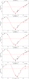 |
Fig. A.1 Example of the fit to the light curves for HV 854. The name filter is listed at the top, as well as the period to the right at the top. The red lines indicate the model fit and the mean value. Crosses indicate points that were flagged as outliers and excluded from the fit. |
The data were fitted with the code described and used in Groenewegen (2004); Groenewegen et al. (2020); Groenewegen (2022) tailored to the Walraven data. The light curves are analysed using a fixed period, fitting for the mean and the amplitude. Depending on the number of available data points the first harmonic period was added in the fit, solving for its amplitude as well. The mean and total amplitude are reported in Table A.2. To the error in the mean a value of 0.015 is added in quadrature. The first entries (HV 824 - 5655) are the stars with new observations, the latter part (HDE 270100 - HV 12815) are the stars from van Genderen (1983) (and van Genderen & Nitihardjo 1989 for HDE 270100) with any new data added in the analysis. An example of the fit to the light curves is shown in Fig. A.1.
Walraven photometry (first entries).
Results of the light curve fitting. Mean VBLUW photometry (first entries).
Appendix B Mass estimates
Table B.1 compiles the mass estimates using the different methods outlined in the main text (also see the table footnote). The adopted mass is the median among the five estimates. To estimate the error bar the error in the mass estimate of the median value is added in quadrature to the median-absolute-deviation times 1.48 (to get the equivalent of one sigma in a Gaussian distribution) among the five estimates.
Stellar mass estimates (selected entries only).
Appendix C 2D Cepheid model
Vasilyev et al. (2017, 2018) present the results of a two-dimensional time-dependent envelope model of a CC with Teff = 5600 K and log ɡ0 = 2.0 dex. In Figure 5 of Vasilyev et al. (2017), the term  is plotted against time. The time series of various quantities were kindly made available, and are plotted in a slightly different way in Fig. C.1. A Fourier analysis of the velocity time series showed a periodicity of 2.6426 days (and a mean of −7.86 km s−1), which is used to phase the data. Phase zero is taken at the instance in time when the normalised flux reaches a maximum for the first time. Consecutive pulsation cycles are plotted with different colours. The cycles are not very smooth. This is explained by convection, which adds statistical fluctuations to the velocity and thermal structure of their model (Sect. 2.1 in Vasilyev et al. 2017).
The integral of the velocity curve is used to calculate the change in radius. For a mass of 3 M⊙, log ɡ = 2.0 dex implies a radius of about 29 R⊙. The top panel shows how ɡeff changes over the pulsation cycle. The effective gravity is below 100 for 68% of the time, with an average value of 66 cm/s2 (−0.18 dex), and above 100 cm/s2 32% of the time for an average of 166 (+0.22 dex). The 5 and 95% percentiles correspond to values of ±0.35 dex. The effect of the change in radius is almost negligible (of order 5-10 cm/s2, or ±0.04 dex at most) compared to the derivative of the velocity in determining ɡeff.
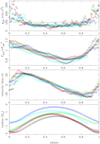 |
Fig. C.1 Various quantities plotted against phase based on the 2D models of Vasilyev et al. (2017, 2018). Different pulsation cycles are plotted in different colours. From top to bottom, the effective gravity, normalised flux, velocity and change in radius. See text for details. |
Appendix D Additional figures
 |
Fig. D.2 Models without dust (left-hand side) with dust (right-hand side) for the five MC stars where the dust excess is unlikely to be related to the star, and the model for the MW star LS Pup for comparison. |
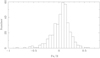 |
Fig. D.3 Distribution in [Fe/H] of the 380 galactic CC used in G20 to determine the PL and PR relations. |
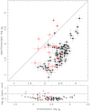 |
Fig. D.4 FWG determined from the SED fitting and the derived stellar mass compared to that from spectroscopic temperature and gravity determination from the literature. Symbols as in Fig. 9. The median offset is −0.79 ± 0.24 dex. |
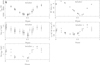 |
Fig. D.7 Same as Fig. 11, but for β Dor. Effective gravities below zero are unphysical and are plotted with a cross at the lowest observed log g. |
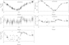 |
Fig. D.8 Same as Fig. 11, but for ζ Gem. Dynamical terms larger than 50 cm/s2 in absolute values are discarded and plotted with a cross. Effective gravities below zero are unphysical and are plotted with a cross at the lowest observed log g. |
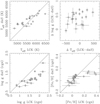 |
Fig. D.9 Comparison between Luck (2018) (LCK) and da Silva et al. (2022) (daS) in terms of effective temperature, log ɡ, the differential between the two, and iron abundance. The stars with only one spectrum in Luck (2018) are marked by circles, objects plotted with squares have 5 or more spectra. Abundances in Luck (2018) are given on a scale where log Hydrogen abundance = 12 and have been converted to the scale in da Silva et al. (2022) using their adopted iron abundance of log Fe = 7.50. |
References
- Anderson, R. I., Saio, H., Ekström, S., Georgy, C., & Meynet, G. 2016, A&A, 591, A8 [NASA ADS] [CrossRef] [EDP Sciences] [Google Scholar]
- Bianchi, L., Shiao, B., & Thilker, D. 2017, ApJS, 230, 24 [Google Scholar]
- Bono, G., Caputo, F., Cassisi, S., et al. 2000a, ApJ, 543, 955 [NASA ADS] [CrossRef] [Google Scholar]
- Bono, G., Castellani, V., & Marconi, M. 2000b, ApJ, 529, 293 [Google Scholar]
- Breitfelder, J., Mérand, A., Kervella, P., et al. 2016, A&A, 587, A117 [CrossRef] [EDP Sciences] [Google Scholar]
- Bresolin, F., Kudritzki, R.-P., & Urbaneja, M. A. 2022, ApJ, 940, 32 [NASA ADS] [CrossRef] [Google Scholar]
- Breuval, L., Riess, A. G., Kervella, P., Anderson, R. I., & Romaniello, M. 2022, ApJ, 939, 89 [NASA ADS] [CrossRef] [Google Scholar]
- Castelli, F., & Kurucz, R. L. 2003, in Modelling of Stellar Atmospheres, 210, eds. N. Piskunov, W. W. Weiss, & D. F. Gray, A20 [NASA ADS] [Google Scholar]
- Chown, A. H., Scowcroft, V., & Wuyts, S. 2021, MNRAS, 500, 817 [Google Scholar]
- Cioni, M.-R. L., Clementini, G., Girardi, L., et al. 2011, A&A, 527, A116 [CrossRef] [EDP Sciences] [Google Scholar]
- Cutri, R. M., et al. 2014, VizieR Online Data Catalog: 2328, 0 [Google Scholar]
- da Silva, R., Crestani, J., Bono, G., et al. 2022, A&A, 661, A104 [NASA ADS] [CrossRef] [EDP Sciences] [Google Scholar]
- de Ruiter, H. R., & Lub, J. 1986, A&AS, 63, 59 [NASA ADS] [Google Scholar]
- De Somma, G., Marconi, M., Cassisi, S., et al. 2021, MNRAS, 508, 1473 [NASA ADS] [CrossRef] [Google Scholar]
- Eggen, O. J. 1977, ApJS, 34, 33 [NASA ADS] [CrossRef] [Google Scholar]
- Gaia Collaboration (Prusti, T., et al.) 2016, A&A, 595, A1 [NASA ADS] [CrossRef] [EDP Sciences] [Google Scholar]
- Gaia Collaboration (Vallenari, A., et al.) 2023, A&A, 674, A1 [NASA ADS] [CrossRef] [EDP Sciences] [Google Scholar]
- Gallenne, A., Kervella, P., & Mérand, A. 2012, A&A, 538, A24 [NASA ADS] [CrossRef] [EDP Sciences] [Google Scholar]
- Gallenne, A., Mérand, A., Kervella, P., et al. 2013, A&A, 558, A140 [NASA ADS] [CrossRef] [EDP Sciences] [Google Scholar]
- Gallenne, A., Kervella, P., Mérand, A., et al. 2017, A&A, 608, A18 [NASA ADS] [CrossRef] [EDP Sciences] [Google Scholar]
- Graczyk, D., Pietrzyński, G., Thompson, I. B., et al. 2020, ApJ, 904, 13 [Google Scholar]
- Groenewegen, M. A. T. 2004, A&A, 425, 595 [NASA ADS] [CrossRef] [EDP Sciences] [Google Scholar]
- Groenewegen, M. A. T. 2012, A&A, 543, A36 [NASA ADS] [CrossRef] [EDP Sciences] [Google Scholar]
- Groenewegen, M. A. T. 2013, A&A, 550, A70 [NASA ADS] [CrossRef] [EDP Sciences] [Google Scholar]
- Groenewegen, M. A. T. 2018, A&A, 619, A8 [NASA ADS] [CrossRef] [EDP Sciences] [Google Scholar]
- Groenewegen, M. A. T. 2020a, A&A, 635, A33 [EDP Sciences] [Google Scholar]
- Groenewegen, M. A. T. 2020b, A&A, 640, A113 [NASA ADS] [CrossRef] [EDP Sciences] [Google Scholar]
- Groenewegen, M. A. T. 2022, A&A, 659, A145 [NASA ADS] [CrossRef] [EDP Sciences] [Google Scholar]
- Groenewegen, M. A. T., & Jurkovic, M. I. 2017, A&A, 604, A29 [NASA ADS] [CrossRef] [EDP Sciences] [Google Scholar]
- Groenewegen, M. A. T., Nanni, A., Cioni, M. R. L., et al. 2020, A&A, 636, A48 [NASA ADS] [CrossRef] [EDP Sciences] [Google Scholar]
- Gustafsson, B., Edvardsson, B., Eriksson, K., et al. 2008, A&A, 486, 951 [NASA ADS] [CrossRef] [EDP Sciences] [Google Scholar]
- Ita, Y., Onaka, T., Tanabé, T., et al. 2010, PASJ, 62, 273 [NASA ADS] [Google Scholar]
- Ivezić, Ž., Nenkova, M., & Elitzur, M. 1999, DUSTY: Radiation transport in a dusty environment, Astrophysics Source Code Library [Google Scholar]
- Kato, D., Ita, Y., Onaka, T., et al. 2012, AJ, 144, 179 [CrossRef] [Google Scholar]
- Kervella, P., Mérand, A., Perrin, G., & Coudé du Foresto, V. 2006, A&A, 448, 623 [NASA ADS] [CrossRef] [EDP Sciences] [Google Scholar]
- Kim, D.-W., Protopapas, P., Bailer-Jones, C. A. L., et al. 2014, A&A, 566, A43 [CrossRef] [EDP Sciences] [Google Scholar]
- Kudritzki, R. P., Bresolin, F., & Przybilla, N. 2003, ApJ, 582, L83 [Google Scholar]
- Kudritzki, R.-P., Urbaneja, M. A., Bresolin, F., et al. 2008, ApJ, 681, 269 [NASA ADS] [CrossRef] [Google Scholar]
- Kudritzki, R. P., Castro, N., Urbaneja, M. A., et al. 2016, ApJ, 829, 70 [NASA ADS] [CrossRef] [Google Scholar]
- Kudritzki, R.-P., Urbaneja, M. A., & Rix, H.-W. 2020, ApJ, 890, 28 [NASA ADS] [CrossRef] [Google Scholar]
- Lemasle, B., Groenewegen, M. A. T., Grebel, E. K., et al. 2017, A&A, 608, A85 [NASA ADS] [CrossRef] [EDP Sciences] [Google Scholar]
- Lindegren, L., Hernández, J., Bombrun, A., et al. 2018, A&A, 616, A2 [NASA ADS] [CrossRef] [EDP Sciences] [Google Scholar]
- Lindegren, L., Bastian, U., Biermann, M., et al. 2021, A&A, 649, A4 [EDP Sciences] [Google Scholar]
- Luck, R. E. 2018, AJ, 156, 171 [Google Scholar]
- Macri, L. M., Ngeow, C.-C., Kanbur, S. M., Mahzooni, S., & Smitka, M. T. 2015, AJ, 149, 117 [Google Scholar]
- Madore, B. F. 1975, ApJS, 29, 219 [Google Scholar]
- Madore, B. F. 1982, ApJ, 253, 575 [NASA ADS] [CrossRef] [Google Scholar]
- Marconi, M., Molinaro, R., Ripepi, V., Musella, I., & Brocato, E. 2013, MNRAS, 428, 2185 [Google Scholar]
- Marconi, M., Molinaro, R., Ripepi, V., et al. 2017, MNRAS, 466, 3206 [NASA ADS] [CrossRef] [Google Scholar]
- Marconi, M., De Somma, G., Ripepi, V., et al. 2020, ApJ, 898, L7 [Google Scholar]
- Martin, W. L., & Warren, P. R. 1979, South Afr. Astron. Observatory Circ., 1, 98 [Google Scholar]
- Mérand, A., Kervella, P., Coudé du Foresto, V., et al. 2006, A&A, 453, 155 [CrossRef] [EDP Sciences] [Google Scholar]
- Mérand, A., Kervella, P., Breitfelder, J., et al. 2015, A&A, 584, A80 [NASA ADS] [CrossRef] [EDP Sciences] [Google Scholar]
- Molinaro, R., Ripepi, V., Marconi, M., et al. 2012, ApJ, 748, 69 [NASA ADS] [CrossRef] [Google Scholar]
- Musella, I., Marconi, M., Stetson, P. B., et al. 2016, MNRAS, 457, 3084 [CrossRef] [Google Scholar]
- Nardetto, N., Fokin, A., Mourard, D., et al. 2004, A&A, 428, 131 [CrossRef] [EDP Sciences] [Google Scholar]
- Nardetto, N., Mérand, A., Mourard, D., et al. 2016, A&A, 593, A45 [CrossRef] [EDP Sciences] [Google Scholar]
- Onken, C. A., Wolf, C., Bessell, M. S., et al. 2019, PASA, 36, e033 [Google Scholar]
- Pel, J. W., van Genderen, A. M., & Lub, J. 1981, A&A, 99, A1 [NASA ADS] [Google Scholar]
- Persson, S. E., Madore, B. F., Krzemiński, W., et al. 2004, AJ, 128, 2239 [NASA ADS] [CrossRef] [Google Scholar]
- Pietrzyński, G., Graczyk, D., Gallenne, A., et al. 2019, Nature, 567, 200 [Google Scholar]
- Pilecki, B., Gieren, W., Pietrzyński, G., et al. 2018, ApJ, 862, 43 [NASA ADS] [CrossRef] [Google Scholar]
- Ragosta, F., Marconi, M., Molinaro, R., et al. 2019, MNRAS, 490, 4975 [NASA ADS] [CrossRef] [Google Scholar]
- Recio-Blanco, A., de Laverny, P., Palicio, P. A., et al. 2023, A&A, 674, A29 [NASA ADS] [CrossRef] [EDP Sciences] [Google Scholar]
- Riess, A. G., Casertano, S., Yuan, W., et al. 2018, ApJ, 861, 126 [NASA ADS] [CrossRef] [Google Scholar]
- Riess, A. G., Casertano, S., Yuan, W., Macri, L. M., & Scolnic, D. 2019, ApJ, 876, 85 [Google Scholar]
- Riess, A. G., Casertano, S., Yuan, W., et al. 2021, ApJ, 908, L6 [NASA ADS] [CrossRef] [Google Scholar]
- Riess, A. G., Yuan, W., Macri, L. M., et al. 2022, ApJ, 934, L7 [NASA ADS] [CrossRef] [Google Scholar]
- Ripepi, V., Marconi, M., Moretti, M. I., et al. 2016, ApJS, 224, 21 [Google Scholar]
- Ripepi, V., Cioni, M.-R. L., Moretti, M. I., et al. 2017, MNRAS, 472, 808 [Google Scholar]
- Ripepi, V., Molinaro, R., Musella, I., et al. 2019, A&A, 625, A14 [NASA ADS] [CrossRef] [EDP Sciences] [Google Scholar]
- Ripepi, V., Chemin, L., Molinaro, R., et al. 2022, MNRAS, 512, 563 [NASA ADS] [CrossRef] [Google Scholar]
- Ripepi, V., Clementini, G., Molinaro, R., et al. 2023, A&A 674, A17 [NASA ADS] [CrossRef] [EDP Sciences] [Google Scholar]
- Romaniello, M., Primas, F., Mottini, M., et al. 2008, A&A, 488, 731 [NASA ADS] [CrossRef] [EDP Sciences] [Google Scholar]
- Romaniello, M., Riess, A., Mancino, S., et al. 2022, A&A, 658, A29 [NASA ADS] [CrossRef] [EDP Sciences] [Google Scholar]
- Sebo, K. M., Rawson, D., Mould, J., et al. 2002, ApJS, 142, 71 [NASA ADS] [CrossRef] [Google Scholar]
- Skowron, D. M., Skowron, J., Udalski, A., et al. 2021, ApJS, 252, 23 [Google Scholar]
- Soszyński, I., Udalski, A., Szymański, M. K., et al. 2017, Acta Astron., 67, 103 [NASA ADS] [Google Scholar]
- Sprague, D., Culhane, C., Kounkel, M., et al. 2022, AJ, 163, 152 [NASA ADS] [CrossRef] [Google Scholar]
- Storm, J., Gieren, W., Fouqué, P., et al. 2011, A&A, 534, A95 [NASA ADS] [CrossRef] [EDP Sciences] [Google Scholar]
- Trahin, B. 2019, PhD thesis, Université PSL, Observatoire de Paris, France [Google Scholar]
- Trahin, B., Breuval, L., Kervella, P., et al. 2021, A&A, 656, A102 [NASA ADS] [CrossRef] [EDP Sciences] [Google Scholar]
- Trundle, C., Dufton, P. L., Hunter, I., et al. 2007, A&A, 471, 62 [Google Scholar]
- Udalski, A., Szymanski, M., Kubiak, M., et al. 1998, Acta Astron., 48, 147 [NASA ADS] [Google Scholar]
- Udalski, A., Szymanski, M., Kubiak, M., et al. 2000, Acta Astron., 50, 307 [NASA ADS] [Google Scholar]
- Ulaczyk, K., Szymański, M. K., Udalski, A., et al. 2012, Acta Astron., 62, 247 [NASA ADS] [Google Scholar]
- Ulaczyk, K., Szymański, M. K., Udalski, A., et al. 2013, Acta Astron., 63, 159 [NASA ADS] [Google Scholar]
- Urbaneja, M. A., Kudritzki, R. P., Gieren, W., et al. 2017, AJ, 154, 102 [NASA ADS] [CrossRef] [Google Scholar]
- van der Marel, R. P., & Kallivayalil, N. 2014, ApJ, 781, 121 [Google Scholar]
- van Genderen, A. M. 1981, A&A, 101, 289 [NASA ADS] [Google Scholar]
- van Genderen, A. M. 1983, A&AS, 52, 423 [NASA ADS] [Google Scholar]
- van Genderen, A. M., & Nitihardjo, G. H. 1989, A&A, 221, 230 [NASA ADS] [Google Scholar]
- Vasilyev, V., Ludwig, H. G., Freytag, B., Lemasle, B., & Marconi, M. 2017, A&A, 606, A140 [NASA ADS] [CrossRef] [EDP Sciences] [Google Scholar]
- Vasilyev, V., Ludwig, H. G., Freytag, B., Lemasle, B., & Marconi, M. 2018, A&A, 611, A19 [NASA ADS] [CrossRef] [EDP Sciences] [Google Scholar]
- Walraven, T., & Walraven, J. H. 1960, Bull. Astron. Inst. Netherlands, 15, 67 [NASA ADS] [Google Scholar]
See the publically available information on ESO program 0109.D-0846(A) (P.I. M. Romaniello) as per October 1st, 2022 and https://www.stsci.edu/hst/phase2-public/17097.pro (P.I. A. Riess), respectively.
https://irsa.ipac.caltech.edu/applications/Gator/, “SAGE MIPS 24 um Epoch 1 and Epoch 2 Full List.”
The complete set of SEDs is available at https://doi.org/10.5281/zenodo.8032168
Cases where the excess consisted only in a single point, typically in the WISE3 filter are not discussed here. They are probably related to contamination in the larger W3 (and W4) beams. An a-priori selection on photometric error in the W3 and W4 filters was applied (Sect. 3.1) but this did not remove all likely unreliable points. The stars discussed in the main text appear to have IR excess in multiple filters.
All Tables
All Figures
|
Fig. 1 Four best-fitting models. The upper panels: Observations (with error bars) and the model. The lower panels: Residuals. Outliers that have been clipped are plotted with an (arbitrary) error bar of 3.0 mag. |
| In the text | |
|
Fig. 2 Comparison of effective temperature and luminosity between the present work and the 27 LMC (filled circles) and 8 SMC (open circles) stars in overlap. The bottom panels show the residuals. |
| In the text | |
|
Fig. 3 Hertzsprung-Russell diagram. Black and red open squares indicate LMC and SMC CCs from the sample, respectively. Stars located outside the bulk of objects are plotted with error bars, and some are labelled as well. Blue symbols with error bars indicate the six CCs in EBs (three FM as filled squares, three FO as filled triangles, see Table 2). Blue and red lines indicate the blue and red edge of the IS. In the upper part (brighter than log L = 3), the results from De Somma et al. (2021) are plotted. The thinner solid and dot-dashed line are for Z = 0.008 and Z = 0.004 models, respectively, for their type A mass-luminosity relation. The tick line is for Z = 0.008 for their type-B mass-luminosity relation. In the lower part (fainter than log L = 3.5), the results from Pilecki et al. (2018) are plotted for FM (solid lines) and FO (dotted lines) model. Green lines indicate evolutionary models from Anderson et al. (2016). See the main text for details. |
| In the text | |
|
Fig. 4 Best-fitting model without dust (left side) and with dust (right side) for the star with the most convincing presence of an IR excess. In the model without dust, the long-wavelength points are considered outliers. |
| In the text | |
|
Fig. 5 Period-Mbol relation. Error bars in Mbol are plotted but are typically smaller than the symbol size. LMC objects are plotted as open squares, SMC objects are filled squares. Blue symbols indicate the six CCs in EBs. One outlier is marked by a red cross and is identified. The black line indicates the best fit (excluding the outlier) to the complete MC sample. Fits to the LMC and SMC stars separately are given in the text. The blue line gives the PL relation for MW CCs from G20, while the red line gives the recommended solution for T2C (Groenewegen 2020a). |
| In the text | |
|
Fig. 6 Zero point at 10 days of the PL-relation for SMC, LMC, and MW. The line is a linear fit with a slope (0.0082 ± 0.0076) mag dex−1 which is not significant. |
| In the text | |
|
Fig. 7 Period-radius relation. LMC objects are plotted as open squares, SMC objects are filled squares. Blue symbols indicate the six CCs in EBs. Outliers removed from the fit are marked by a red cross and some are identified. The black line indicates the best fit (excluding the outliers) to the complete MC sample. Fits to the LMC and SMC stars separately are given in the text. The blue line gives the PR relation for MW CCs from G20. |
| In the text | |
|
Fig. 8 Mass-luminosity relation. Objects in the LMC are plotted as black, those in the SMC as red open squares. Stars outside the bulk of objects are identified. Objects in blue are the known CCs and their companions in EBs. The blue line indicates the canonical ML relation from Bono et al. (2000a) for Y = 0.255 and Z = 0.008. For Z = 0.004 the line would be at higher luminosities by about 0.1 dex. The black line indicates a fit to the LMC stars minus the outliers (see Eq. (12)) and lies almost exactly +0.3 dex above the canonical ML relation. |
| In the text | |
|
Fig. 9 Comparison between the effective temperatures determined from the SED fitting and in the literature. Objects in the LMC are plotted in black and objects in the SMC in red. The one-to-one line is indicated. Stars where the absolute difference is larger than 1000 K are identified. Objects from reference 1 and 2 (see the note to Table 1) are plotted as filled squares, from reference 3 as open squares, from reference 4 as filled triangles, from reference 5 as open triangles, and from reference 6 as filled circles. In the lower panel, the difference between literature and photometric temperature is plotted. |
| In the text | |
|
Fig. 10 Comparison between the log ɡ determined in the literature, and the evolutionary value as determined from L and Teff from the SED fitting and the stellar mass based on various methods (see Appendix B). The one-to-one line is indicated. Stars outside the bulk of objects are identified. Symbols as in Fig. 9. |
| In the text | |
|
Fig. 11 Time series of effective temperature, radial velocity and gravity for δ Cep from da Silva et al. (2022). Calculated in the presented paper are the dynamical term and the effective gravity based on the mean gravity and the dynamical term. The ordinate for the effective gravity is set to that of the observed gravity. |
| In the text | |
|
Fig. 12 FWG versus log P. Black points indicate the FWGs derived from L and Teff (from the SED fitting) and stellar mass in the present paper. Black open squares are LMC objects, filled squares indicate SMC objects. Blue symbols indicate the CCs (filled squares) and one T2C (filled triangle) in EB systems. The black line is a fit to the black points, minus the two marked outliers. The red circles indicate FWGs from HR spectroscopy (open circles indicate LMC, filled circles indicate SMC), Light blue filled squares indicate FWGs of 20 MC CCs from da Silva et al. (2022), while the green points indicate the FWGs for the same 20 objects from Luck (2018; open squares indicate that only one spectrum is available in Luck 2018, filled squares indicate that five or more spectra are available). |
| In the text | |
|
Fig. 13 FWGLR: LMC and SMC objects are identified by black and red open squares. To avoid cluttering the plot, representative error bars are plotted for the smallest and largest values of log ɡF only. Some outliers are marked, and stars excluded from the fit are marked by a red cross. Blue filled squares indicate the six EB CCs and their companions, the filled red square indicates the T2C in the LMC-T2CEP-098 system and the filled black square its companion. The black line gives the best fit to the objects (Eq. (16)). The green line at small FWGs is the fit to LMC BSGs (Urbaneja et al. 2017; Bresolin et al. 2022). |
| In the text | |
|
Fig. A.1 Example of the fit to the light curves for HV 854. The name filter is listed at the top, as well as the period to the right at the top. The red lines indicate the model fit and the mean value. Crosses indicate points that were flagged as outliers and excluded from the fit. |
| In the text | |
|
Fig. C.1 Various quantities plotted against phase based on the 2D models of Vasilyev et al. (2017, 2018). Different pulsation cycles are plotted in different colours. From top to bottom, the effective gravity, normalised flux, velocity and change in radius. See text for details. |
| In the text | |
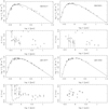 |
Fig. D.1 Details as in Fig. 1 for the four poorest-fitting models. |
| In the text | |
|
Fig. D.2 Models without dust (left-hand side) with dust (right-hand side) for the five MC stars where the dust excess is unlikely to be related to the star, and the model for the MW star LS Pup for comparison. |
| In the text | |
|
Fig. D.3 Distribution in [Fe/H] of the 380 galactic CC used in G20 to determine the PL and PR relations. |
| In the text | |
|
Fig. D.4 FWG determined from the SED fitting and the derived stellar mass compared to that from spectroscopic temperature and gravity determination from the literature. Symbols as in Fig. 9. The median offset is −0.79 ± 0.24 dex. |
| In the text | |
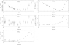 |
Fig. D.5 Same as Fig. 11, but for T Vul. |
| In the text | |
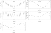 |
Fig. D.6 Same as Fig. 11, but for FF Aql. |
| In the text | |
|
Fig. D.7 Same as Fig. 11, but for β Dor. Effective gravities below zero are unphysical and are plotted with a cross at the lowest observed log g. |
| In the text | |
|
Fig. D.8 Same as Fig. 11, but for ζ Gem. Dynamical terms larger than 50 cm/s2 in absolute values are discarded and plotted with a cross. Effective gravities below zero are unphysical and are plotted with a cross at the lowest observed log g. |
| In the text | |
|
Fig. D.9 Comparison between Luck (2018) (LCK) and da Silva et al. (2022) (daS) in terms of effective temperature, log ɡ, the differential between the two, and iron abundance. The stars with only one spectrum in Luck (2018) are marked by circles, objects plotted with squares have 5 or more spectra. Abundances in Luck (2018) are given on a scale where log Hydrogen abundance = 12 and have been converted to the scale in da Silva et al. (2022) using their adopted iron abundance of log Fe = 7.50. |
| In the text | |
Current usage metrics show cumulative count of Article Views (full-text article views including HTML views, PDF and ePub downloads, according to the available data) and Abstracts Views on Vision4Press platform.
Data correspond to usage on the plateform after 2015. The current usage metrics is available 48-96 hours after online publication and is updated daily on week days.
Initial download of the metrics may take a while.