| Issue |
A&A
Volume 699, July 2025
|
|
|---|---|---|
| Article Number | A102 | |
| Number of page(s) | 17 | |
| Section | Interstellar and circumstellar matter | |
| DOI | https://doi.org/10.1051/0004-6361/202554369 | |
| Published online | 04 July 2025 | |
The spectral energy distributions of very long-period Cepheids in the Milky Way, the Magellanic Clouds, M31, and M33
Koninklijke Sterrenwacht van België,
Ringlaan 3,
1180
Brussels,
Belgium
★ Corresponding author: This email address is being protected from spambots. You need JavaScript enabled to view it.
Received:
4
March
2025
Accepted:
13
May
2025
Abstract
The spectral energy distributions (SEDs) of 20 Milky Way (MW), 9 Large Magellanic Cloud (LMC), 7 Small Magellanic Cloud (SMC), 12 M31, and 7 M33 (classical) Cepheids with periods longer than 50 days were constructed using photometric data from the literature and fitted with model atmospheres with the aim of identifying objects with an infrared excess. The SEDs were fitted with stellar photosphere models to derive the best-fitting luminosity and effective temperature; a dust component was added when required. The distance and reddening values were taken from the literature. WISE and IRC images were inspected to verify whether potential excess emission was related to the central objects. Only one star with a significant infrared (IR) excess was found in the LMC and none in the SMC, M31, and M33, contrary to earlier work on the MW suggesting that IR excess may be more prominent in MW Cepheids than in the Magellanic Clouds. One additional object in the MW was found to have an IR excess, but it is unclear whether it is a classical Cepheid or a type-II Cepheid. The stars were plotted in a Hertzsprung-Russell diagram (HRD) and compared to evolutionary tracks for CCs and to theoretical instability strips. For the large majority of stars, the position in the HRD is consistent with the instability strip. For stars in the MW uncertainties in the distance and reddening can significantly change their position in the HRD.
Key words: stars: distances / stars: fundamental parameters / stars: variables: Cepheids
© The Authors 2025
 Open Access article, published by EDP Sciences, under the terms of the Creative Commons Attribution License (https://creativecommons.org/licenses/by/4.0), which permits unrestricted use, distribution, and reproduction in any medium, provided the original work is properly cited.
This article is published in open access under the Subscribe to Open model. This email address is being protected from spambots. You need JavaScript enabled to view it. to support open access publication.
1 Introduction
Classical Cepheids (CCs) are important standard candles because they are bright and provide a link between the distance scale in the nearby universe and that further out via those galaxies that contain both Cepheids and SNIa (see Riess et al. 2022 and Murakami et al. 2023 for a determination of the Hubble constant to 1.0 km s−1 precision or better). Typically, the periodluminosity (PL) relations of CCs that are at the core of the distance determinations are derived in particular photometric filters (V, I, K) or combinations of filters that are designed to be reddening independent, called the Wesenheit functions (Madore 1982), for example using combinations of (V, I) or (J, K), or the combination used by the SH0ES team (F555W, F814W, and F160W HST filters; see Riess et al. 2022).
On the other hand, the bolometric magnitude or luminosity is a fundamental quantity of stars as it is the output of stellar evolution models and the input to CC pulsation models. This is the continuation of a series of papers that construct and analyse the spectral energy distributions (SEDs) of CCs. in Groenewegen (2020a) (hereafter G20) the SEDs of 477 Galactic CCs were constructed and fitted with model atmospheres (and a dust component when required). For an adopted distance (from Gaia DR2 at that time), reddening these fits resulted in a best-fitting bolometric luminosity (L) and the photometrically derived effective temperature (Teff). This allowed the derivation of period-radius (PR) and period-luminosity (PL) relations, the construction of the Hertzsprung-Russell diagram (HRD), and a comparison to theoretical instability strips (iSs). This sample was further studied in Groenewegen (2020b), where the relation was investigated between the bolometric absolute magnitude and the flux-weighted gravity (FWG); this is known as the flux-weighted gravity-luminosity relation (FWGLR).
In Groenewegen & Lub (2023) 77 Small Magellanic Cloud (SMC) and 142 Large Magellanic Cloud (LMC) CCs were studied along similar lines. The advantage of using the Magellanic Clouds (MCs) is that accurate and independently derived mean distances are available based on the analysis of samples of eclipsing binaries (Pietrzyński et al. 2019; Graczyk et al. 2020).
Interestingly, in the latter study, only one case was found where there was evidence of an infrared excess, namely the longest period object in the LMC. This is in contrast to Galactic CCs where near-iR (NiR) and mid-iR (MiR) excess is known to exist, revealed for example via direct interferometric observations in the optical or NiR (e.g. Kervella et al. 2006; Mérand et al. 2006; Gallenne et al. 2012; Nardetto et al. 2016; Hocdé et al. 2025b), modelling with the SPiPS code (e.g. Breitfelder et al. 2016; Trahin 2019; Trahin et al. 2021, and Gallenne et al. 2017 for the LMC) and was also found in modelling of the SEDs of Galactic CCs (Gallenne et al. 2013; G20).
This raises the question of whether this apparent difference in the presence of IR excess could be related to metallicity. To investigate this further, a complete sample of long-period Cepheids (periods longer than 50 days; see below) is studied in this paper, in the MW, the MCs, and M31 and M33. This study is connected to the class of ultra long-period (ULP) Cepheids, a term introduced by Bird et al. (2009) as fundamental mode (FU) Cepheids with periods longer than 80 days (see reviews by Musella et al. 2021 and Musella 2022 specifically on ULPs).
The paper is structured as follows. in Section 2, the sample of Cepheids is introduced, while Section 3 introduces the photometry that is used, the distances used, and how the modelling of the SED was done. Section 4 discusses several results, in particular the location of the objects in the HRD, the presence of infrared excess, the PR and PL relations, and models with alternative distances or reddenings. A brief discussion and summary concludes the paper in Sect. 5.
Adopted distances.
2 Sample
For this paper a sample of55 Cepheids was studied. In particular the sample is compiled from the following:
Galactic Cepheids from Pietrukowicz et al. (2021)1 which contains 3666 CCs. The longest period listed there is S Vul with a period of 68.65 d, clearly shorter than the classical limit of 80 days for ULPs. An (arbitrary) lower limit of 50 days is used, which results in nine objects.
SMC and LMC CCs from the OGLE-IV catalogue (Soszyński et al. 2019), resulting in six and eight objects, respectively, with periods longer than 50 days.
From the Gaia DR3 vari_cepheid table all CCs with a period longer than 50 days and type DCEP were selected, for a total of 53 objects (Ripepi et al. 2023; Gaia Collaboration 2023, 2016).
All of the sources from Pietrukowicz et al. (2021) are in the vari_cepheid table, except OGLE-GD-CEP-1505. It is listed there, but classified as a Type-II Cepheid (T2C) of the RV Tau class. It was kept in the sample as our analysis may shed light on its nature. All of the sources from Soszyński et al. (2019) are in the vari_cepheid table, except OGLE-LMC-CEP-4689. This is the well-known variable HV 2827, listed in the Gaia main catalogue, but not in the Gaia Cepheid and vari_summary tables. The source is kept. Thirty-one sources from the vari_cepheid table are not in the samples from Pietrukowicz et al. (2021) and Soszyński et al. (2019).
The 55 sources were matched with the SIMBAD database to obtain additional names and identifiers. Twelve objects are likely members of M31 and seven are likely members of M33. The remaining 20 appear to be in the Milky Way. Five of them are in the direction of the Galactic Bulge and four of these have been classified as T2C by the OGLE team.
Basic information of the 55 stars are compiled in Table A.1. All LMC objects except LMC-Dachs2-24, and all SMC objects except SMC-Dachs3-5 and SMC-CEP-1977 were studied by Groenewegen & Lub (2023), while S Vul and GY Sge were studied in G20. However, the analysis of the SEDs was repeated here independently. It should be noted that there are known CCs in other galaxies with periods longer than 50 days (see e.g. Musella 2022), but they are not included in the Gaia vari_cepheid table.
As for some sources there is a possible confusion about whether they are CCs or T2C of the RV Tau type, Cols. 8 and 9 give the predicted luminosity for the two classes based on the LMC PL relations of Groenewegen & Lub (2023) and Groenewegen & Jurkovic (2017), respectively. Typically, these luminosities differ by a factor of 20-30 for periods in the range 50-200 days, implying changes in distance by a factor of 5 to ‘convert’ a T2C into a CC, or vice versa, purely based on consistency with a PL relation.
3 Photometry, distance, masses, and modelling
3.1 Photometry
The SEDs were constructed using photometry retrieved mostly, but not exclusively, via the VizieR web-interface2. Table B.1 lists the filters and references to the photometry that were considered. An additional reason for not considering known CCs with periods longer than 50 days in more distant galaxies is that there are less (and less accurate) MIR data available, which are needed to detect an IR excess, and the problem of contamination or blending as a given beam size or aperture corresponds to a larger physical size (as indeed turns out to be the case for some objects, see Sect. 4.3). The data contain single-epoch observations (typically from GALEX and Akari) but whenever possible values at mean light were taken or multiple data points were averaged.
3.2 Distance and geometric correction
For the LMC, M31, and M33, mean distances from the literature were adopted and a geometric correction was applied to correct for the fact that the sources are to first order located in an inclined disc, following Grocholski et al. (2007). The depth effect in the SMC is considerable (e.g. Ripepi et al. 2017), and all SMC sources were adopted tobe at the mean distance. For the Galactic Bulge region3 the distance from the GRAVITY experiment was adopted (GRAVITY Collaboration 2022). For the remainder of the MW sources the geometric distance from Bailer-Jones et al. (2021) was adopted. Details and references are listed in Table 1. The distances to the individual sources are given in Table A.2.
The 3D reddening maps of Lallement et al. (2022) and Vergely et al. (2022) were used4 to obtain the AV in a given direction as well as the distance to which this reddening refers. For the sources in M31 and M33 a value of AV = 0.17 was adopted which is the average value from the 3D reddening map at the largest available distance in the direction of those galaxies. For the MCs the reddening map of Skowron et al. (2021) was used and the E(V − I) value in the map closest to the source is taken. The visual extinction was then taken as AV = 3.1 · E(V − I)/1.318, following Skowron et al. (2021). The reddenings to the individual sources are given in Table A.2.
3.3 Modelling
The SEDs are fitted with the code More of DUSTY (MoD, Groenewegen 2012)5, which uses a slightly updated and modified version of the DUSTY dust radiative transfer (RT) code (Ivezić et al. 1999) as a subroutine within a minimisation code. The dust optical depth is initially set to zero. In that case the inputs to the model are the distance, reddening, and a model atmosphere. The cases where an infrared (IR) excess may be present are discussed in Sect. 4.3.
The MARCS model atmospheres are used as input (Gustafsson et al. 2008) for log g = 1.5 and for adopting canonical metallicities of −0.50 and −0.75 dex for the LMC and SMC stars, and +0.00 for M31, M33, the Bulge, and the MW sources6. The model grid was available at 250 K intervals for the effective temperature range of interest, and adjacent model atmospheres were used to interpolate models at 125 K intervals, which more closely reflects the accuracy in Teff that can be achieved. For every model atmosphere (that is, Teff) a best-fitting luminosity (with its [internal] error bar, based on the covariance matrix) is derived with the corresponding reduced χ2 ( ) of the fit. The model with the lowest
  then gives the best-fitting effective temperature. Considering models within a certain range above this minimum
  then gives the estimated error in the effective temperature and luminosity. For the luminosity this error is added in quadrature to the internal error in luminosity.
In the model fitting procedure photometric outliers were excluded in the following way. The photometric error bar for each data point was added in quadrature to 1.4826 · median absolute deviation (MAD) of the residuals in the fit to give the equivalent of 1σ in a Gaussian distribution. If the absolute difference between the model and observations was larger than 4σ, the point was flagged and plotted with an error bar of 3.0 mag so that it was still identified, but had no influence on the fitting. The model grid over temperatures was run again, and the clipping procedure repeated. Then the run over effective temperatures was repeated a last time. The best-fitting effective temperature and luminosity with error bars are listed in Table A.2.
4 Results
4.1 General
Figure 1 shows some best fits without considering dust. This illustrates the quality of the modelling with the residual (model minus observations) in the bottom part of each panel7.
4.2 Hertzsprung-Russell diagram
Figure 2 shows the HRD together with sets of evolutionary tracks and the ISs of CCs in two panels. Objects from the sample are plotted as filled squares (SMC), open squares (LMC), open triangles (M31), filled triangles (M33), filled circles (Galactic Bulge), and open circles (MW). Stars located outside the bulk of objects are plotted with error bars and some are labelled as well. The red and blue edges of the IS of CCs are plotted for Z = 0.015 and 0.004 (De Somma et al. 2021). The near horizontal green lines indicate the evolutionary tracks of CCs for Z = 0.014 and average initial rotation rate ωini = 0.5 from Anderson et al. (2016). Increasing in luminosity are tracks for initial mass (the number of the crossing through the IS): 4 (1), 5 (1), 5 (2), 5 (3), 7 (1), 7 (2), 7 (3), 9 (1), 9 (2), 9 (3), 12 (1), and 15 M⊙ (1). The blue and pink crosses in the left panel indicate the MIST evolutionary tracks for 5.0, 10, and 17 M⊙ (for [Fe/H]= 0.0 dex) and 4.8, 9, and 15 M⊙ (for [Fe/H]= −0.50 dex), respectively, plotted at 104 year intervals (Dotter 2016; Choi et al. 2016; Paxton et al. 2015, 2013, 2011). The 4.8 and 5.0 M⊙ tracks are the lowest mass ones with blue loops that reach the IS of CCs.
The right panel focusses on the T2C, and the black and red crosses respectively indicate the evolutionary tracks of 1.0 and 2.5 M⊙ solar metallicity stars, including the post-AGB phase, plotted at 103 year intervals (from Vassiliadis & Wood 1994). In addition, triangles and diamonds indicate T2C with periods longer than 50 days in the MCs (from Groenewegen & Jurkovic 2017) and the MW (from Bódi & Kiss 2019), respectively.
In the left panel there is a clear separation between objects whose location is consistent with the IS of CCs, and those that are clearly cooler, and in almost all cases, are significantly less luminous. Most of them have been classified as T2C in the literature. It is noted that 4 of the 12 CCs in M31 are close to the red edge of the IS for Z = 0.03. Based on the MIST and Anderson et al. (2016) evolutionary models the CCs have masses in the ~10-15 M⊙ range.
The right panel, which focusses on the T2C region shows that the location of the stars in the sample is different from the known MCs and MW T2Cs with periods longer than 50 days from Groenewegen & Jurkovic (2017) and Bódi & Kiss (2019). The selection was very different in the sense that the latter studies started from samples of T2C, while the stars in this sample were initially believed to be largely CCs. Six objects have luminosities that lie above or close to the post-AGB track for a 1 M track, but seven do not. These objects are most probably postRGB objects (see Kamath et al. 2016), although they are not dusty. Among the potential T2Cs only II Car shows some evidence of the presence of dust (see Sect. 4.3), all the others are well fit by a stellar atmosphere and do not show the characteristic disc or shell IR signature in their SEDs.
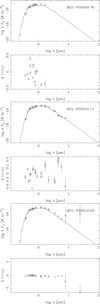 |
Fig. 1 Examples of best-fitting models assuming no dust. The upper panels show the observations (with error bars) and the model. The lower panel shows the residuals. Outliers that have been clipped are plotted with an (arbitrary) error bar of 3.0 mag. |
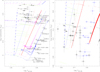 |
Fig. 2 Hertzsprung-Russell diagram. The left panel presents an overview while the red panel focusses on the T2Cs. The symbols are follows: filled squares (SMC), open squares (LMC), open triangles (M31), filled triangles (M33), filled circles (Galactic Bulge), and open circles (MW). Stars located outside the bulk of objects are identified. The blue and red lines indicate the blue and red edge of the IS of CCs. The results from De Somma et al. (2021) are plotted for Z = 0.03 (thick solid lines) and Z = 0.004 models (thinner dashed lines), for their type A mass-luminosity relation. The green lines indicate evolutionary models from Anderson et al. (2016) (see text for details). The blue and pink crosses indicate MIST evolutionary tracks for v/vcrit = 0.4 for 5.0, 10, and 17 M⊙ (and [Fe/H]= 0.0 dex) and 4.8, 9, and 15 M⊙ (and [Fe/H]= −0.50 dex), respectively, plotted at 104 year intervals (Dotter 2016; Choi et al. 2016; Paxton et al. 2015, 2013, 2011). The first crossing of the IS is also visible, except for the highest mass tracks. In the right panel the objects in the sample are plotted in blue, without names and the MIST evolutionary tracks are not shown. Instead, the black and red crosses indicate the evolutionary tracks of the 1.0 and 2.5 M⊙ solar metallicity stars, respectively, including the post-AGB phase, plotted at 103 year intervals (from Vassiliadis & Wood 1994). For comparison, the black triangles and spades indicate T2C with periods longer than 50 days in the MCs (from Groenewegen & Jurkovic 2017) and the MW (from Bódi & Kiss 2019), respectively. GD-CEP-1505 is located outside both plots at log Teff ~ 3.48 and log L ~ 2.18. |
Results of the fitting of dust models.
4.3 Infrared excess
The default assumption in the modelling was that there is no IR excess and the SEDs can be modelled by a stellar atmosphere. However, NIR and MIR excess are known to exist in Galactic CCs, for example direct interferometric observations in the optical or NIR and other methods (see references quoted in the Introduction), and one possibility to explain the IR excess is through dust emission. For T2Cs dust emission is a very plausible explanation as the long period T2C are associated with the RV Tau variability class that are generally believed to be in the post-AGB evolutionary phase (e.g. Manick et al. 2018).
In a next step, models were run with the dust optical depth (τd, at 0.5 μm) and dust temperature at the inner radius (Td) as additional fit parameters. The dust shell was assumed to be spherically symmetric. Models with different initial guesses were run (Td starting from 250, 400, 600, 800, 1000, and 1500 K; τd starting from 0.1, 0.3, 0.6, and 1). The Bayesian information criterion (BIC; Schwarz 1978) was used as a first check to determine whether a model with dust fitted the SED better than a model atmosphere. However, some flexibility in a strict application was needed as some seemingly better models converged to Td values higher than the effective temperature, or had an error bar on Td of the same order as Td. In addition, the initial set of models was run for an effective temperature that resulted from the models without dust. A model with dust will increase the flux in the infrared due to emission but it will also absorb radiation in the optical, and therefore the best-fitting effective temperature will likely become higher. It should be pointed out that for a few objects (M31-PSO009.76, shown in Fig. 1, M33-013331, M33-V00021, and M33-013405) there is no photometry available beyond the NIR. As the contrast between the emission by dust and the stellar photosphere increases with wavelength this is not ideal to detect any excess emission; the absence of proof for infrared excess is not the proof of absence.
Based on these considerations, additional models were run for 9 stars out of the 55 in the sample, where the effective temperature was allowed to vary as well. For one star the results were not deemed conclusive (M33-013305) and the best-fitting models including dust for eight stars are listed in Table 2, one star each in the MW, LMC, and M33, and five in M31. Figure 3 compares the best-fitting models with and without dust for two objects, while the six others are shown in Fig. C.1. Table 2 includes the BIC of models under three model assumptions; the SEDs fitted including a dust component, a model without dust and where photometric outliers were removed (the model in Table A.2), and a model without dust and including all data points. The last model clearly represents the worst fit. In six cases the BIC of the model including dust is lower than the model without the outliers. Comparing the reduced χ2 (Col. 4 in Table 2 to Col. 6 in Table A.2) this is only the case for two objects.
To further investigate the nature of the IR excess and to check the possibility that the IR excess is not associated with the CCs but related to diffuse background, the emission images from the ALLWISE survey8 and the Spitzer Enhanced Imaging Products (SEIP)9 were inspected. Figure C.2 and Figure C.3 show images in the WISE W1 and W3, and IRAC 1 and 4 filters, respectively, around selected CCs. The two objects in the top rows are different examples of stars without IR excess that are located in empty fields. The other panels show the eight stars with an IR excess in the SEDs from Table 2. Except for II Car and LMC-CEP-0619, the emission of the stars at the longest WISE3 and IRAC4 wavelengths (when detected) seems not be clearly associated with the central star, but appears to be diffuse emission or possibly partly blended. In the cases of M31-PSO010.63, M31-GDR369249, M31-VRJ004357, M31-PSO011.09, M31-VRJ004434, and M33-013312 the correct model is the standard model without dust and not considering the photometric outliers because these are very likely not associated with the objects.
4.4 Alternative models for the MW
For objects in the Bulge and MW, uncertainties in the adopted distance and reddening are important limitations in deriving accurate luminosities and photometric effective temperatures (also see G20). Table A.2 includes the distance and AV estimates from Anders et al. (2022) based on the StarHorse code (Queiroz et al. 2018) that are independent from the initially adopted distances from Bailer-Jones et al. (2021) and the 3D reddening model.
Models for the 20 MW and BUL stars were rerun based on the parameters from StarHorse or, when not available, on plausible estimates based on general 1σ error bars in the distance and on plausible extrapolations of the reddening. The finally adopted parameters and the resulting best fits are listed in Table A.3. Figure 4 compares the standard models with the best-fitting models including dust or the alternative distances and reddenings. Especially for some of the MW objects the change in luminosity and effective temperature are large (e.g. for GDR404357), while the fit quality remains almost unchanged, indicating that the two parameters are degenerate. While for some stars the alternative models move the object closer to or inside the IS, the location in the HRD of S Vul is moved outside the IS. A special case is GD-CEP-1505. The alternative model is an improvement, but the fit is still the poorest of all stars. Fixing the effective temperature to 4000 K and choosing a distance of 4.0 kpc will result in a luminosity of 1350 L, a position consistent with the other T2Cs in the sample and the luminosity predicted for its period, but requires a very high reddening of AV = 11 for its Galactic position of l = +47.09, b = +0.90. Table A.3 also includes some relevant quantities from the Gaia main catalogue, namely the G-band magnitude, the parallax, the goodness-of-fit parameter (GoF, expected to follow a Gaussian distribution centred on zero and with width unity), and the renormalised unit weight error (expected to be centred on unity).
The standard adopted distance from Bailer-Jones et al. (2021) uses the observed parallax, the parallax zero point correction from Lindegren et al. (2021), and a prior constructed from a three-dimensional model of the Galaxy to determine the distance and error. A few CCs are located outside the IS, which could point to a distance that is different from that in Bailer-Jones et al. (2021) or the alternative distance. The parallax zero point correction is more uncertain for G magnitudes ≲ 12.5 (e.g. Cruz Reyes & Anderson 2023), the significance of the parallaxes, π/σπ, is often only 1-3 so that the prior will have a large impact on the derived distance, and some of the astrometric solutions are poor (RUWE ≳ 1.4 or |GoF| ≳ 3). Gaia DR4 is expected to deliver more accurate parallaxes that could resolve these issues.
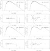 |
Fig. 3 Examples of best-fitting models assuming dust (right) compared to no dust (left panels). We note the difference in the range of the ordinate in the left and right bottom panels. The other six objects are shown in Fig. C.1. In the models without dust some photometric points are considered outliers and are plotted with a large error bar, instead of omitting them. |
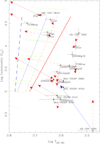 |
Fig. 4 Hertzsprung-Russell diagram. The symbols and lines largely follow Fig. 2. The standard models are connected to the best-fitting alternative models (i.e. with dust or alternative distances and reddenings) by a red line with arrow. The arrow is dashed when the alternative model has a reduced χ2 that is lower by 10% or more than that of the standard model, dot-dashed when the alternative model has a reduced χ2 that is larger by 10% or more, and solid otherwise. The blue line for GD-CEP-1505 indicates yet another alternative model (see text). |
4.5 Period-luminosity and period-radius relations
Figure 5 shows the PL and PR relations based on the standard model results, together with the PL and PR relations for CCs and T2Cs from Groenewegen & Lub (2023) and Groenewegen & Jurkovic (2017) for the LMC. The alternative models have not been plotted as they do not change the overall picture. These relations confirm largely what is also seen in the HRD. Some stars are located in these diagrams in positions consistent with their being T2Cs, but for some this is true for the PR diagram, but not for the PL diagram. There is more scatter in the relations for T2C than for CCs, but this is related to the fact that most of the CCs are located in external galaxies with better defined distances and reddenings than for the MW and Bulge objects.
Table 3 shows the classification of the 20 MW and Bulge objects based on the position in the HRD, the PL, and the PR diagrams. All ten that were previously classified or re-classified by the Gaia team as T2C are confirmed as such. GD-CEP-1505 is most definitely not a CC. It is most likely a T2C, but for its effective temperature and luminosity to be consistent with this requires a distance and reddening that is very different from that derived in the literature. Six stars are certainly CCs, and for four stars the results are not conclusive.
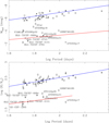 |
Fig. 5 Period-Mbol and PR relations. The error bars in Mbol are plotted but are typically smaller than the symbol size. The symbols are follows: filled squares (SMC), open squares (LMC), open triangles (M31), filled triangles (M33), filled circles (Galactic Bulge), and open circles (MW). Stars located outside the bulk of objects are identified. The blue lines give the relation for LMC CCs from Groenewegen & Lub (2023) while the red lines give the recommended solution for LMC T2Cs from Groenewegen & Jurkovic (2017). GD-CEP-1505 is located outside the upper plot at log P ~ 1.7 and Mbol –0.6 mag. |
5 Discussion and summary
Table 4 summarises the results of the SED fitting of G20, Groenewegen & Lub (2023), and this paper in terms of the likely presence of IR excess emission based on the SED fitting. The numbers for the MW for P > 50 d depend on whether II Car and some of the other objects are considered CC or T2C (see Table 3).
The fraction of CCs with IR excess appears small with the notable exception of the shorter period MW objects (~5%). In view of the Hubble tension (e.g. Perivolaropoulos 2024) it is an interesting question whether the presence of IR excess could impact the derivation of the CC PL relation, especially if the effect were different in the calibrating galaxies and in the galaxies the relation is applied to. The current analysis suggests that the impact should be low at best. Among the Galactic sample studied by Riess et al. (2021) in their preferred HST F555W, F814W, and F160W filter system to calibrate the PL-relation, only S TrA and HW Car possibly have an IR excess, and LMC619 is not among the calibrating sample of 70 LMC CCs studied in Riess et al. (2019).
Nevertheless, the presence and the origin of an IR excess remains intriguing and requires further study. Although it was assumed in the modelling that this is due to dust this origin is problematic (how 1000 K dust can form around a 6000 K central star; see discussion in G20) and free-free emission from ionised gas seems a viable alternative Hocdé et al. (2020a,b, 2025a). Interferometric observations of the MW stars that are claimed to have IR excess emission based on SED modelling would provide additional constraints. An alternative would be to obtain MIR spectroscopy which would also be done for CCs in the LMC. Even at a low resolution of ~50 any silicate dust feature would become detectable and, if absent, any continuum emission over that expected from the stellar photosphere would put constraints on the underlying mechanism.
T2C and CC classification.
Detection of IR excess.
Data availability
The complete set of SEDs of the standard models and the alternative models is available at http://doi.org/10.5281/zenodo.15422721
Acknowledgements
This work has made use of data from the European Space Agency (ESA) mission Gaia (http://www.cosmos.esa.int/gaia), processed by the Gaia Data Processing and Analysis Consortium (DPAC, http://www.cosmos.esa.int/web/gaia/dpac/consortium). Funding for the DPAC has been provided by national institutions, in particular the institutions participating in the Gaia Multilateral Agreement. This research has used data, tools or materials developed as part of the EXPLORE project that has received funding from the European Union’s Horizon 2020 research and innovation programme under grant agreement No 101004214. This research uses services or data provided by the Astro Data Lab at NSF’s National Optical-Infrared Astronomy Research Laboratory. NOIRLab is operated by the Association of Universities for Research in Astronomy (AURA), Inc. under a cooperative agreement with the National Science Foundation. This research has made use of the SIMBAD database and the VizieR catalogue access tool operated at CDS, Strasbourg, France.
Appendix A Sample and fitting results
Sample of stars
Results of the fitting without dust
Results of the fitting using alternative distances and reddenings, and some Gaia parameters
Appendix B Sources of the photometry
Photometry used to construct the SEDs
Appendix C Additional figures
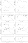 |
Fig. C.1 Best-fitting models assuming dust (right-hand) compared to no dust (left-hand panels) of the remaining 6 objects (cf. Fig. 3). Note the difference in the range of the ordinate in the left-hand and right-hand bottom panels. |
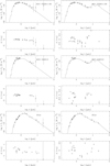 |
Fig. C.1 continued. |
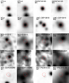 |
Fig. C.2 Cut-outs of about 1′ × 1′ (45×45 pixels of 1.37″) in the W1 and W3 filters centred on the CC. Cut levels are at the 0.5 and 99.5% level. The red circle marks the nominal position and has a radius of 5 pixels, corresponding to approximately 1 FWHM of the point spread function. ET Vul and GDR 6746185 are plotted for comparison as MW stars not having an IR excess. |
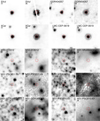 |
Fig. C.3 Cut-outs of about 30″ x 30″ (51x51 pixels of 0.60″) in the IRAC 1 and 4 filters centred on the CC. Cut levels are at the 0.5 and 99.5% level. The red circle marks the nominal position and has a radius of 3 pixels, corresponding to approximately 1 FWHM of the point spread function. S Vul and GDR 404357 are plotted for comparison as MW stars not having an IR excess. |
References
- Anders, F., Khalatyan, A., Queiroz, A. B. A., et al. 2022, A&A, 658, A91 [NASA ADS] [CrossRef] [EDP Sciences] [Google Scholar]
- Anderson, R. I., Saio, H., Ekström, S., Georgy, C., & Meynet, G. 2016, A&A, 591, A8 [NASA ADS] [CrossRef] [EDP Sciences] [Google Scholar]
- Bailer-Jones, C. A. L., Rybizki, J., Fouesneau, M., Demleitner, M., & Andrae, R. 2021, AJ, 161, 147 [Google Scholar]
- Beichmann, C. A. 1985, Infrared Astronomical Satellite (IRAS) catalogs and atlases. Explanatory supplement [Google Scholar]
- Berdnikov, L. N. 2008, VizieR Online Data Catalog: II/285 [Google Scholar]
- Berdnikov, L. N., Kniazev, A. Y., Sefako, R., et al. 2015, VizieR Online Data Catalog: J/PAZh/41/27 [Google Scholar]
- Bianchi, L., Shiao, B., & Thilker, D. 2017, ApJS, 230, 24 [Google Scholar]
- Bird, J. C., Stanek, K. Z., & Prieto, J. L. 2009, ApJ, 695, 874 [Google Scholar]
- Bódi, A., & Kiss, L. L. 2019, ApJ, 872, 60 [CrossRef] [Google Scholar]
- Breitfelder, J., Mérand, A., Kervella, P., et al. 2016, A&A, 587, A117 [CrossRef] [EDP Sciences] [Google Scholar]
- Breuval, L., Riess, A. G., Macri, L. M., et al. 2023, ApJ, 951, 118 [CrossRef] [Google Scholar]
- Chambers, K. C., Magnier, E. A., Metcalfe, N., et al. 2016, arXiv e-prints [arXiv:1612.05560] [Google Scholar]
- Chen, X., Wang, S., Deng, L., et al. 2020, ApJS, 249, 18 [NASA ADS] [CrossRef] [Google Scholar]
- Choi, J., Dotter, A., Conroy, C., et al. 2016, ApJ, 823, 102 [Google Scholar]
- Chown, A. H., Scowcroft, V., & Wuyts, S. 2021, MNRAS, 500, 817 [Google Scholar]
- Cioni, M.-R. L., Clementini, G., Girardi, L., et al. 2011, A&A, 527, A116 [CrossRef] [EDP Sciences] [Google Scholar]
- Cruz Reyes, M., & Anderson, R. I. 2023, A&A, 672, A85 [NASA ADS] [CrossRef] [EDP Sciences] [Google Scholar]
- Cutri, R. M., et al. 2014, VizieR Online Data Catalog: II/328 [Google Scholar]
- Cutri, R. M., Skrutskie, M. F., van Dyk, S., et al. 2003, VizieR Online Data Catalog: II/246 [Google Scholar]
- Cutri, R. M., Skrutskie, M. F., van Dyk, S., et al. 2012, VizieR Online Data Catalog: II/281 [Google Scholar]
- Dalcanton, J. J., Williams, B. F., Lang, D., et al. 2012, ApJS, 200, 18 [Google Scholar]
- Denis, C. 2005, VizieR Online Data Catalog: B/denis [Google Scholar]
- De Somma, G., Marconi, M., Cassisi, S., et al. 2021, MNRAS, 508, 1473 [NASA ADS] [CrossRef] [Google Scholar]
- Dotter, A. 2016, ApJS, 222, 8 [Google Scholar]
- Drew, J. E., Gonzalez-Solares, E., Greimel, R., et al. 2014, MNRAS, 440, 2036 [Google Scholar]
- Drew, J. E., Gonzales-Solares, E., Greimel, R., et al. 2016, VizieR Online Data Catalog: II/341 [Google Scholar]
- Egan, M. P., Price, S. D., Kraemer, K. E., et al. 2003, VizieR Online Data Catalog: V/114 [Google Scholar]
- Eggen, O. J. 1977, ApJS, 34, 33 [NASA ADS] [CrossRef] [Google Scholar]
- Gaia Collaboration (Prusti, T., et al.) 2016, A&A, 595, A1 [NASA ADS] [CrossRef] [EDP Sciences] [Google Scholar]
- Gaia Collaboration (Vallenari, A., et al.) 2023, A&A, 674, A1 [NASA ADS] [CrossRef] [EDP Sciences] [Google Scholar]
- Gallenne, A., Kervella, P., & Mérand, A. 2012, A&A, 538, A24 [NASA ADS] [CrossRef] [EDP Sciences] [Google Scholar]
- Gallenne, A., Mérand, A., Kervella, P., et al. 2013, A&A, 558, A140 [NASA ADS] [CrossRef] [EDP Sciences] [Google Scholar]
- Gallenne, A., Kervella, P., Mérand, A., et al. 2017, A&A, 608, A18 [NASA ADS] [CrossRef] [EDP Sciences] [Google Scholar]
- Graczyk, D., Pietrzynski, G., Thompson, I. B., et al. 2020, ApJ, 904, 13 [Google Scholar]
- GRAVITY Collaboration (Abuter, R., et al.) 2021, A&A, 647, A59 [NASA ADS] [CrossRef] [EDP Sciences] [Google Scholar]
- GRAVITY Collaboration (Abuter, R., et al.) 2022, A&A, 657, L12 [NASA ADS] [CrossRef] [Google Scholar]
- Grocholski, A. J., Sarajedini, A., Olsen, K. A. G., Tiede, G. P., & Mancone, C. L. 2007, AJ, 134, 680 [Google Scholar]
- Groenewegen, M. A. T. 2012, A&A, 543, A36 [NASA ADS] [CrossRef] [EDP Sciences] [Google Scholar]
- Groenewegen, M. A. T. 2020a, A&A, 635, A33 [EDP Sciences] [Google Scholar]
- Groenewegen, M. A. T. 2020b, A&A, 640, A113 [NASA ADS] [CrossRef] [EDP Sciences] [Google Scholar]
- Groenewegen, M. A. T., & Jurkovic, M. I. 2017, A&A, 604, A29 [NASA ADS] [CrossRef] [EDP Sciences] [Google Scholar]
- Groenewegen, M. A. T., & Lub, J. 2023, A&A, 676, A136 [NASA ADS] [CrossRef] [EDP Sciences] [Google Scholar]
- Gustafsson, B., Edvardsson, B., Eriksson, K., et al. 2008, A&A, 486, 951 [NASA ADS] [CrossRef] [EDP Sciences] [Google Scholar]
- Gutermuth, R. A., & Heyer, M. 2015, AJ, 149, 64 [Google Scholar]
- Henden, A. A., Levine, S., Terrell, D., & Welch, D. L. 2015, in American Astronomical Society Meeting Abstracts, 225, 336.16 [Google Scholar]
- Herschel PSC Working Group, Marton, G., Calzoletti, L., et al. 2020, VizieR Online Data Catalog: VIII/106 [Google Scholar]
- Hocdé, V., Nardetto, N., Lagadec, E., et al. 2020a, A&A, 633, A47 [NASA ADS] [CrossRef] [EDP Sciences] [Google Scholar]
- Hocdé, V., Nardetto, N., Borgniet, S., et al. 2020b, A&A, 641, A74 [EDP Sciences] [Google Scholar]
- Hocdé, V., Kaminski, T., Lewis, M., et al. 2025a, A&A, 694, L15 [NASA ADS] [CrossRef] [EDP Sciences] [Google Scholar]
- Hocdé, V., Matter, A., Nardetto, N., et al. 2025b, A&A, 694, A101 [NASA ADS] [CrossRef] [EDP Sciences] [Google Scholar]
- Ishihara, D., Onaka, T., Kataza, H., et al. 2010, A&A, 514, A1 [NASA ADS] [CrossRef] [EDP Sciences] [Google Scholar]
- Ita, Y., Onaka, T., Tanabé, T., et al. 2010, PASJ, 62, 273 [NASA ADS] [Google Scholar]
- Ivezić, Z., Nenkova, M., & Elitzur, M. 1999, DUSTY: Radiation transport in a dusty environment, Astrophysics Source Code Library [record ascl:9911.001] [Google Scholar]
- Javadi, A., van Loon, J. T., & Mirtorabi, M. T. 2011, MNRAS, 411, 263 [Google Scholar]
- Kamath, D., Wood, P. R., Van Winckel, H., & Nie, J. D. 2016, A&A, 586, L5 [NASA ADS] [CrossRef] [EDP Sciences] [Google Scholar]
- Kato, D., Ita, Y., Onaka, T., et al. 2012, AJ, 144, 179 [CrossRef] [Google Scholar]
- Kervella, P., Mérand, A., Perrin, G., & Coudé du Foresto, V. 2006, A&A, 448, 623 [NASA ADS] [CrossRef] [EDP Sciences] [Google Scholar]
- Khan, R. 2017, ApJS, 228, 5 [NASA ADS] [CrossRef] [Google Scholar]
- Khan, R., Stanek, K. Z., Kochanek, C. S., & Sonneborn, G. 2015, ApJS, 219, 42 [NASA ADS] [CrossRef] [Google Scholar]
- Kourkchi, E., Courtois, H. M., Graziani, R., et al. 2020, AJ, 159, 67 [NASA ADS] [CrossRef] [Google Scholar]
- Lallement, R., Vergely, J. L., Babusiaux, C., & Cox, N. L. J. 2022, A&A, 661, A147 [NASA ADS] [CrossRef] [EDP Sciences] [Google Scholar]
- Laney, C. D., & Stobie, R. S. 1992, A&AS, 93, 93 [NASA ADS] [Google Scholar]
- Li, S., Riess, A. G., Busch, M. P., et al. 2021, ApJ, 920, 84 [NASA ADS] [CrossRef] [Google Scholar]
- Li, Y., Jiang, B., & Ren, Y. 2025, AJ, 170, 2 [Google Scholar]
- Lindegren, L., Bastian, U., Biermann, M., et al. 2021, A&A, 649, A4 [EDP Sciences] [Google Scholar]
- Ma, B., Shang, Z., Hu, Y., et al. 2018, MNRAS, 479, 111 [Google Scholar]
- Madore, B. F. 1975, ApJS, 29, 219 [Google Scholar]
- Madore, B. F. 1982, ApJ, 253, 575 [NASA ADS] [CrossRef] [Google Scholar]
- Manick, R., Van Winckel, H., Kamath, D., Sekaran, S., & Kolenberg, K. 2018, A&A, 618, A21 [NASA ADS] [CrossRef] [EDP Sciences] [Google Scholar]
- Marocco, F., Eisenhardt, P. R. M., Fowler, J. W., et al. 2021, ApJS, 253, 8 [Google Scholar]
- Martin, W. L., & Warren, P. R. 1979, South Afr. Astron. Observ. Circ., 1, 98 [Google Scholar]
- Massey, P., Neugent, K. F., & Smart, B. M. 2016, AJ, 152, 62 [NASA ADS] [CrossRef] [Google Scholar]
- McMahon, R. G., Banerji, M., Gonzalez, E., et al. 2013, The Messenger, 154, 35 [NASA ADS] [Google Scholar]
- Mérand, A., Kervella, P., Coudé du Foresto, V., et al. 2006, A&A, 453, 155 [CrossRef] [EDP Sciences] [Google Scholar]
- Minniti, D., Lucas, P. W., Emerson, J. P., et al. 2010, New A, 15, 433 [Google Scholar]
- Monson, A. J., & Pierce, M. J. 2011, ApJS, 193, 12 [Google Scholar]
- Murakami, Y. S., Riess, A. G., Stahl, B. E., et al. 2023, J. Cosmology Astropart. Phys., 2023, 046 [Google Scholar]
- Musella, I. 2022, Universe, 8, 335 [NASA ADS] [CrossRef] [Google Scholar]
- Musella, I., Marconi, M., Molinaro, R., et al. 2021, MNRAS, 501, 866 [Google Scholar]
- Nardetto, N., Mérand, A., Mourard, D., et al. 2016, A&A, 593, A45 [CrossRef] [EDP Sciences] [Google Scholar]
- Neugent, K. F., Massey, P., Georgy, C., et al. 2020, ApJ, 889, 44 [NASA ADS] [CrossRef] [Google Scholar]
- Nidever, D. L., Olsen, K., Choi, Y., et al. 2021, AJ, 161, 74 [NASA ADS] [CrossRef] [Google Scholar]
- Paxton, B., Bildsten, L., Dotter, A., et al. 2011, ApJS, 192, 3 [Google Scholar]
- Paxton, B., Cantiello, M., Arras, P., et al. 2013, ApJS, 208, 4 [Google Scholar]
- Paxton, B., Marchant, P., Schwab, J., et al. 2015, ApJS, 220, 15 [Google Scholar]
- Pel, J. W. 1976, A&AS, 24, 413 [NASA ADS] [Google Scholar]
- Pellerin, A., & Macri, L. M. 2011, ApJS, 193, 26 [NASA ADS] [CrossRef] [Google Scholar]
- Perivolaropoulos, L. 2024, Phys. Rev. D, 110, 123518 [Google Scholar]
- Pietrukowicz, P., Soszyńcski, I., & Udalski, A. 2021, Acta Astron., 71, 205 [NASA ADS] [Google Scholar]
- Pietrzync ski, G., Graczyk, D., Gallenne, A., et al. 2019, Nature, 567, 200 [NASA ADS] [CrossRef] [Google Scholar]
- Queiroz, A. B. A., Anders, F., Santiago, B. X., et al. 2018, MNRAS, 476, 2556 [Google Scholar]
- Riess, A. G., Casertano, S., Yuan, W., Macri, L. M., & Scolnic, D. 2019, ApJ, 876, 85 [Google Scholar]
- Riess, A. G., Casertano, S., Yuan, W., et al. 2021, ApJ, 908, L6 [NASA ADS] [CrossRef] [Google Scholar]
- Riess, A. G., Yuan, W., Macri, L. M., et al. 2022, ApJ, 934, L7 [NASA ADS] [CrossRef] [Google Scholar]
- Ripepi, V., Marconi, M., Moretti, M. I., et al. 2016, ApJS, 224, 21 [Google Scholar]
- Ripepi, V., Cioni, M.-R. L., Moretti, M. I., et al. 2017, MNRAS, 472, 808 [Google Scholar]
- Ripepi, V., Chemin, L., Molinaro, R., et al. 2022, MNRAS, 512, 563 [NASA ADS] [CrossRef] [Google Scholar]
- Ripepi, V., Clementini, G., Molinaro, R., et al. 2023, A&A, 674, A17 [NASA ADS] [CrossRef] [EDP Sciences] [Google Scholar]
- Schwarz, G. 1978, Ann. Stat., 6, 461 [Google Scholar]
- Skowron, D. M., Skowron, J., Udalski, A., et al. 2021, ApJS, 252, 23 [Google Scholar]
- Soszyńcski, I., Udalski, A., Szymancski, M. K., et al. 2017, Acta Astron., 67, 103 [Google Scholar]
- Soszyńcski, I., Udalski, A., Szymancski, M. K., et al. 2019, Acta Astron., 69, 87 [Google Scholar]
- Soszyńcski, I., Udalski, A., Szymancski, M. K., et al. 2020, Acta Astron., 70, 101 [Google Scholar]
- Spitzer Science, C. 2009, VizieR Online Data Catalog: II/293 [Google Scholar]
- Szabados, L. 1977, Mitt. Sternw. Ungarisch. Akad. Wiss, 70 [Google Scholar]
- Szabados, L. 1980, Commun. Konkoly Obs. Hung., 76, 1 [Google Scholar]
- Szabados, L. 1981, Commun. Konkoly Obs. Hung., 77, 1 [Google Scholar]
- Szabados, L. 1991, Commun. Konkoly Obs. Hung., 96, 123 [NASA ADS] [Google Scholar]
- Trahin, B. 2019, PhD thesis, L’Université PSL, l’Observatoire de Paris, France [Google Scholar]
- Trahin, B., Breuval, L., Kervella, P., et al. 2021, A&A, 656, A102 [NASA ADS] [CrossRef] [EDP Sciences] [Google Scholar]
- Udalski, A., Soszync ski, I., Pietrukowicz, P., et al. 2018, Acta Astron., 68, 315 [NASA ADS] [Google Scholar]
- Ulaczyk, K., Szymanc ski, M. K., Udalski, A., et al. 2012, Acta Astron., 62, 247 [Google Scholar]
- Ulaczyk, K., Szymanc ski, M. K., Udalski, A., et al. 2013, Acta Astron., 63, 159 [Google Scholar]
- Vassiliadis, E., & Wood, P. R. 1994, ApJS, 92, 125 [NASA ADS] [CrossRef] [Google Scholar]
- Vergely, J. L., Lallement, R., & Cox, N. L. J. 2022, A&A, 664, A174 [NASA ADS] [CrossRef] [EDP Sciences] [Google Scholar]
- Williams, B. F., Lang, D., Dalcanton, J. J., et al. 2014, ApJS, 215, 9 [Google Scholar]
- Williams, B. F., Durbin, M. J., Dalcanton, J. J., et al. 2021, ApJS, 253, 53 [NASA ADS] [CrossRef] [Google Scholar]
Version dated September 17, 2022 https://www.astrouw.edu.pl/ogle/ogle4/OCVS/allGalCep.listID
Defined as the region with 266 < RA < 270° and −33 < δ < −28° and comprising the four sources with BLG-T2CEP in their names and the source marked GDR404357.
Metallicity gradients in M31 and M33 are not considered (see e.g. Li et al. 2025).
The complete set of SEDs is available at https://doi.org/10.5281/zenodo.15422721
All Tables
Results of the fitting using alternative distances and reddenings, and some Gaia parameters
All Figures
|
Fig. 1 Examples of best-fitting models assuming no dust. The upper panels show the observations (with error bars) and the model. The lower panel shows the residuals. Outliers that have been clipped are plotted with an (arbitrary) error bar of 3.0 mag. |
| In the text | |
|
Fig. 2 Hertzsprung-Russell diagram. The left panel presents an overview while the red panel focusses on the T2Cs. The symbols are follows: filled squares (SMC), open squares (LMC), open triangles (M31), filled triangles (M33), filled circles (Galactic Bulge), and open circles (MW). Stars located outside the bulk of objects are identified. The blue and red lines indicate the blue and red edge of the IS of CCs. The results from De Somma et al. (2021) are plotted for Z = 0.03 (thick solid lines) and Z = 0.004 models (thinner dashed lines), for their type A mass-luminosity relation. The green lines indicate evolutionary models from Anderson et al. (2016) (see text for details). The blue and pink crosses indicate MIST evolutionary tracks for v/vcrit = 0.4 for 5.0, 10, and 17 M⊙ (and [Fe/H]= 0.0 dex) and 4.8, 9, and 15 M⊙ (and [Fe/H]= −0.50 dex), respectively, plotted at 104 year intervals (Dotter 2016; Choi et al. 2016; Paxton et al. 2015, 2013, 2011). The first crossing of the IS is also visible, except for the highest mass tracks. In the right panel the objects in the sample are plotted in blue, without names and the MIST evolutionary tracks are not shown. Instead, the black and red crosses indicate the evolutionary tracks of the 1.0 and 2.5 M⊙ solar metallicity stars, respectively, including the post-AGB phase, plotted at 103 year intervals (from Vassiliadis & Wood 1994). For comparison, the black triangles and spades indicate T2C with periods longer than 50 days in the MCs (from Groenewegen & Jurkovic 2017) and the MW (from Bódi & Kiss 2019), respectively. GD-CEP-1505 is located outside both plots at log Teff ~ 3.48 and log L ~ 2.18. |
| In the text | |
|
Fig. 3 Examples of best-fitting models assuming dust (right) compared to no dust (left panels). We note the difference in the range of the ordinate in the left and right bottom panels. The other six objects are shown in Fig. C.1. In the models without dust some photometric points are considered outliers and are plotted with a large error bar, instead of omitting them. |
| In the text | |
|
Fig. 4 Hertzsprung-Russell diagram. The symbols and lines largely follow Fig. 2. The standard models are connected to the best-fitting alternative models (i.e. with dust or alternative distances and reddenings) by a red line with arrow. The arrow is dashed when the alternative model has a reduced χ2 that is lower by 10% or more than that of the standard model, dot-dashed when the alternative model has a reduced χ2 that is larger by 10% or more, and solid otherwise. The blue line for GD-CEP-1505 indicates yet another alternative model (see text). |
| In the text | |
|
Fig. 5 Period-Mbol and PR relations. The error bars in Mbol are plotted but are typically smaller than the symbol size. The symbols are follows: filled squares (SMC), open squares (LMC), open triangles (M31), filled triangles (M33), filled circles (Galactic Bulge), and open circles (MW). Stars located outside the bulk of objects are identified. The blue lines give the relation for LMC CCs from Groenewegen & Lub (2023) while the red lines give the recommended solution for LMC T2Cs from Groenewegen & Jurkovic (2017). GD-CEP-1505 is located outside the upper plot at log P ~ 1.7 and Mbol –0.6 mag. |
| In the text | |
|
Fig. C.1 Best-fitting models assuming dust (right-hand) compared to no dust (left-hand panels) of the remaining 6 objects (cf. Fig. 3). Note the difference in the range of the ordinate in the left-hand and right-hand bottom panels. |
| In the text | |
|
Fig. C.1 continued. |
| In the text | |
|
Fig. C.2 Cut-outs of about 1′ × 1′ (45×45 pixels of 1.37″) in the W1 and W3 filters centred on the CC. Cut levels are at the 0.5 and 99.5% level. The red circle marks the nominal position and has a radius of 5 pixels, corresponding to approximately 1 FWHM of the point spread function. ET Vul and GDR 6746185 are plotted for comparison as MW stars not having an IR excess. |
| In the text | |
|
Fig. C.3 Cut-outs of about 30″ x 30″ (51x51 pixels of 0.60″) in the IRAC 1 and 4 filters centred on the CC. Cut levels are at the 0.5 and 99.5% level. The red circle marks the nominal position and has a radius of 3 pixels, corresponding to approximately 1 FWHM of the point spread function. S Vul and GDR 404357 are plotted for comparison as MW stars not having an IR excess. |
| In the text | |
Current usage metrics show cumulative count of Article Views (full-text article views including HTML views, PDF and ePub downloads, according to the available data) and Abstracts Views on Vision4Press platform.
Data correspond to usage on the plateform after 2015. The current usage metrics is available 48-96 hours after online publication and is updated daily on week days.
Initial download of the metrics may take a while.