| Issue |
A&A
Volume 685, May 2024
|
|
|---|---|---|
| Article Number | A41 | |
| Number of page(s) | 43 | |
| Section | Stellar structure and evolution | |
| DOI | https://doi.org/10.1051/0004-6361/202348650 | |
| Published online | 06 May 2024 | |
The VMC survey
L. Type II Cepheids in the Magellanic Clouds: Period–luminosity relations in the near-infrared bands⋆,⋆⋆
1
Scuola Superiore Meridionale, Largo S. Marcellino 10, 80138 Napoli, Italy
2
INAF-Osservatorio Astronomico di Capodimonte, Salita Moiariello 16, 80131 Napoli, Italy
e-mail: This email address is being protected from spambots. You need JavaScript enabled to view it.
; This email address is being protected from spambots. You need JavaScript enabled to view it.
3
Leibniz-Institut für Astrophysik Potsdam (AIP), An der Sternwarte 16, 14482 Potsdam, Germany
4
School of Mathematical and Physical Sciences, Macquarie University, Balaclava Road, Sydney, NSW 2109, Australia
5
Astrophysics and Space Technologies Research Centre, Macquarie University, Balaclava Road, Sydney, NSW 2109, Australia
6
International Space Science Institute–Beijing, 1 Nanertiao, Zhongguancun, Hai Dian District, Beijing 100190, PR China
7
Koninklijke Sterrenwacht van België, Ringlaan 3, 1180 Brussels, Belgium
8
European Southern Observatory, Karl-Schwarzschild-Str. 2, 85748 Garching bei München, Germany
9
Istituto Nazionale di Fisica Nucleare (INFN), Sezione di Napoli, Via Cinthia 21, 80126 Napoli, Italy
10
INAF-Osservatorio Astronomico d’Abruzzo, Via Maggini sn, 64100 Teramo, Italy
Received:
17
November
2023
Accepted:
21
January
2024
Abstract
Context. Type II Cepheids (T2Cs) are the less frequently used counterparts of classical or type I Cepheids (CCs) which provide the primary calibration of the distance ladder for measuring the Hubble constant in the local Universe. In the era of the “Hubble tension”, T2C variables together with the RR Lyrae stars and the tip of the red giant branch (TRGB) can potentially provide non-CC-dependent calibration of the cosmic distance ladder.
Aims. Our goal is to provide an absolute calibration of the period–luminosity, period–luminosity–colour, and period–Wesenheit relations (PL, PLC, and PW, respectively) of T2Cs in the Large Magellanic Cloud (LMC), which traditionally serves as a crucial first anchor of the extragalactic distance ladder.
Methods. We exploited time-series photometry in the near-infrared (NIR) Y, J, and Ks bands for a sample of approximately 320 T2Cs in the Magellanic Clouds (MCs). These observations were acquired during 2009–2018 in the context of the VISTA survey of the Magellanic Clouds system (VMC), an ESO public survey. We supplemented the NIR photometry from the VMC survey with well-sampled optical light curves and accurate pulsation periods from the Optical Gravitational Lensing Experiment (OGLE) IV survey and the Gaia mission. We used the best-quality NIR light curves to generate custom templates for modelling sparsely sampled light curves in YJKs bands.
Results. The best-fitting YJKs template light curves were used to derive accurate and precise intensity-averaged mean magnitudes and pulsation amplitudes of 277 and 62 T2Cs in the LMC and SMC, respectively. We used optical and NIR mean magnitudes for different T2C subclasses (BLHer, WVir, and RVTau) to derive PL/PLC/PW relations in multiple bands, which were calibrated with the geometric distance to the LMC as derived from eclipsing binaries and with the Gaia parallaxes. We used our new empirical calibrations of PL and PW relations to obtain distances to 22 T2C-host Galactic globular clusters, which were found to be systematically smaller by ∼0.1 mag and 0.03−0.06 mag than in the literature when the zero points are calibrated with the distance of the LMC or Gaia parallaxes, respectively. Better agreement is found between our distances and those based on RR Lyrae stars in globular clusters, providing strong support for using these population II stars together with the TRGB for future distance scale studies.
Key words: stars: oscillations / stars: Population II / stars: variables: Cepheids / Magellanic Clouds / distance scale
Full Tables 1, 3, 5 and A.1–A.3 are available at the CDS via anonymous ftp to cdsarc.cds.unistra.fr (130.79.128.5) or via https://cdsarc.cds.unistra.fr/viz-bin/cat/J/A+A/685/A41
Based on observations made with VISTA at the Paranal Observatory under program ID 179.B-2003.
© The Authors 2024
 Open Access article, published by EDP Sciences, under the terms of the Creative Commons Attribution License (https://creativecommons.org/licenses/by/4.0), which permits unrestricted use, distribution, and reproduction in any medium, provided the original work is properly cited.
This article is published in open access under the Subscribe to Open model. This email address is being protected from spambots. You need JavaScript enabled to view it. to support open access publication.
1. Introduction
The determination of the Hubble constant (H0), which parametrises the expansion rate of the Universe, is highly debated given the ongoing tension between the H0 values derived from the extragalactic distance scale, traditionally adopting classical Cepheids (CCs) and type Ia supernovae (SNeIa), and those inferred by the Planck mission based on the Λ cold dark matter theory applied to the cosmic microwave background measurements (see e.g. Riess et al. 2022; Planck Collaboration VI 2020). Given this ongoing tension, CC-independent calibration of the cosmic distance ladder using stellar standard candles of different ages and metallicities is being explored to investigate possible sources of systematic uncertainties in H0 determinations. One of the most promising alternative calibrations based on the tip of the red giant branch (TRGB) stars provides an H0 value that is intermediate between Cepheid-Supernovae and Planck measurements (Freedman 2021). Population II stars, such as type II Cepheids (T2Cs) and RR Lyrae variables (RRL), can be used independently or together with the TRGB stars, providing another alternative calibration for the local H0 measurements based on old stellar standard candles.
T2Cs are probably old, low-mass, and metal-poor stars. Based on their pulsation periods, they are separated into three types: (i) BL Herculis (BLHer) stars with periods of between 1 and 4 days; (ii) W Virginis (WVir) stars with periods of between 4 and 20 days; and (iii) RV Tauri (RVTau) stars with periods of between 20 and 150 days. However, these period boundaries are only approximate; especially those between WVir and RVTau stars. Soszyński et al. (2008) noticed a subsample of WVir stars showing peculiar light curves and brighter magnitudes than normal WVir stars of a given period. These peculiar WVir (pWVir) stars are suspected to have a binary origin.
From the evolutionary point of view, BLHer, WVir, and RVTau are thought to be in different evolutionary phases, going from post-horizontal branch (post-HB) to post-asymptotic giant branch (post-AGB, Gingold 1976, 1985). BLHer are low-mass stars that have exhausted their core helium on the portion of the HB bluer than the classical instability strip (IS) populated by RRL. They are ascending towards the AGB phase, becoming increasingly brighter and redder. In this process, BLHer cross the classical IS at luminosities higher than that of the RRL (see e.g. Di Criscienzo et al. 2007; Marconi & Di Criscienzo 2007, and references therein). The WVir stars exhibit a more advanced evolutionary phase than BLHer stars. Indeed, these latter are thought to be AGB stars crossing the IS at higher luminosities (which explains the longer periods) than BLHer stars on the blueward and redward path of the blue loop during the thermal pulse phase (see e.g. Bono et al. 2020; Wallerstein 2002, and references therein). Historically, RVTau stars have been considered to be the post-AGB stars, which cross the IS at even higher luminosities than WVir stars, but recent studies have also suggested a connection to binary evolution (see e.g. Groenewegen & Jurkovic 2017).
T2Cs can be used as distance indicators because they follow very tight period–luminosity, period–Wesenheit1, and period–luminosity–colour relationships (PL, PW and PLC; see e.g. Feast et al. 2008; Matsunaga et al. 2011; Ripepi et al. 2015; Bhardwaj et al. 2017a; Bhardwaj 2020). These empirical relations based on T2Cs are almost parallel to those of CCs but at significantly fainter (i.e. 1−1.5 mag) magnitudes. Ripepi et al. (2015), Bhardwaj et al. (2017a), and Bhardwaj (2022, and references therein) suggested that the RRL PL relations are an extension of the T2C PL relations at shorter periods in the near-infrared (NIR), in agreement with theoretical predictions (see e.g. Caputo et al. 2004; Marconi & Di Criscienzo 2007). In particular, BLHer and WVir stars follow common PL relations in the NIR bands but different PL relations in the optical (e.g. Ripepi et al. 2015; Bhardwaj et al. 2017b, and references therein). The NIR PL relations of short-period T2Cs exhibit less scatter than those of the RVTau stars, especially in the Large Magellanic Cloud (LMC). The NIR PL relations have several advantages compared to the optical bands because of the smaller extinction, lower variability amplitude, and smaller temperature variations associated with them, which lead to tighter PL relations.
The T2Cs are generally found in Galactic globular clusters (GGCs) with blue HB morphology, in all components of the Milky Way, namely the bulge, disc, and halo. However, these stars are rare in dwarf galaxies in the Local Group, except for a few hundred stars in the Magellanic Clouds (MCs; Soszyński et al. 2018) and four in the Sagittarius dwarf spheroidal galaxy (Hamanowicz et al. 2016). The MCs also host standard candles such as CCs (∼11 000) and RRL stars (∼45 000) (e.g. Soszyński et al. 2018; Clementini et al. 2019, 2023; Ripepi et al. 2023). The absolute calibration of NIR PL, PW, and PLC relations for T2Cs in the MCs will be useful for the distance scale because the LMC, and (to a lesser extent) the SMC, have traditionally served as an anchor of the distance ladder (e.g. Riess et al. 2022, and references therein). The simultaneous presence of different standard candles in the same galaxy also allows us to compare the distances obtained with the different indicators, providing a means to look for systematic errors. Particularly important is the homogeneity of the RRL and T2C distance scales, as both types of pulsators can be used to calibrate the TRGB method in an alternative route to calibrate H0 (Beaton et al. 2016).
The LMC and the Small Magellanic Cloud (SMC) comprise the Magellanic system together with the “bridge” connecting them and the “stream”, a H I feature covering more than 100 deg on the sky (e.g. Mathewson et al. 1974). The LMC and the SMC lie at an average distance of ∼50 and 60 kpc, respectively (e.g. Pietrzyński et al. 2019; Graczyk et al. 2020). In the context of the NIR survey of the MCs, a great contribution has been provided by the ESO “Visible and Infrared Survey Telescope for Astronomy” (VISTA) public survey of the Magellanic Clouds system (VMC; Cioni et al. 2011). The main aims of the VMC survey are (i) to reconstruct the spatially resolved star formation history and (ii) to infer an accurate three-dimensional map of the whole Magellanic system. The survey was designed to observe in three bands, Y, J, and Ks, and to obtain deep time-series photometry reaching even the faintest Cepheids of all types and the vast majority of RRLs known in the MCs. The interested readers are referred to Cioni et al. (2011) for details regarding the VMC survey. Time-series YJKs observations from the VMC survey are particularly useful in providing calibration the PL and PW relations of primary stellar standard candles in the MCs.
The NIR PL and PW relations of T2Cs have been explored in different environments: the Galactic bulge (Bhardwaj et al. 2017b; Braga et al. 2018), GGCs (Matsunaga et al. 2006; Bhardwaj 2022; Ngeow et al. 2022), and the MCs (Matsunaga et al. 2011; Ripepi et al. 2015; Bhardwaj et al. 2017a). Several studies, in particular those from the OGLE survey and the Gaia mission, have also investigated PL relations at optical wavelengths (Alcock et al. 1998; Iwanek et al. 2018; Ripepi et al. 2023, and references therein). The accurate and precise parallaxes from the Gaia mission (Gaia Collaboration 2016) have also allowed the calibration of the PL and PW relations based on Galactic field T2Cs in the Gaia bands (Ripepi et al. 2023) and NIR bands (Wielgórski et al. 2022). A small but non-negligible effect of metallicity on the absolute NIR magnitude of T2Cs was found by Matsunaga et al. (2006) and Wielgórski et al. (2022). However, Ngeow et al. (2022) did not find any statistically significant dependence of PL relations on metallicity for T2Cs, in agreement with theoretically predicted relations (Di Criscienzo et al. 2007; Das et al. 2021).
The scope of this work is to take advantage of Data Release 5 and 6 of the VMC survey2 in order to derive new accurate NIR PL and PW relations for the T2C in both the LMC and SMC following previous, similar work by Ripepi et al. (2015). Compared with this latter study, we have more than doubled the sample of T2Cs in the MCs and have at our disposal both a new accurate distance of the LMC (and SMC) and the parallaxes of the Gaia mission Data Release 3 (DR3, Gaia Collaboration 2016, 2023b) for Galactic T2Cs. Overall, we will be able to calculate and calibrate PL and PW relations in the MCs, which will be particularly useful for the distance scale based on population II stars.
2. Type II Cepheids in the VMC survey
The observing strategy of the VMC survey is discussed in detail in Cioni et al. (2011). In brief, the VMC surveyed an area of 184 deg2 covering almost the entire LMC, SMC and Bridge in three bands Y, J and Ks (central wavelength λc = 1.02, 1.25 and 2.15 μm, respectively) using the VIRCAM (VISTA InfraRed CAMera; Dalton et al. 2006; Emerson et al. 2006) instrument attached to the VISTA telescope. The VMC Ks-band time-series observations were planned to obtain 13 different epochs (eleven reaching a limiting magnitude of Ks ∼ 19.3 mag with a S/N ∼ 5, plus two shallower obtained with half of the exposure time) executed over several consecutive months with a specific observing cadence to obtain well-sampled light curves for pulsating variables (for details see Cioni et al. 2011; Ripepi et al. 2012; Moretti et al. 2014). For the Y and J bands, four epochs were planned, of which two were shallower. In practice, the actual number of epochs is larger, as many observations were repeated because of lower quality (i.e. data not matching the observational constraints), even if good enough to build light curves (see e.g. Ripepi et al. 2016).
The raw VISTA images acquired for the VMC survey were reduced by the VISTA Data Flow System (VDFS; Irwin et al. 2004) pipeline at the Cambridge Astronomical Survey Unit (CASU)3. The data used in this work were reduced using version 1.5 of the VDFS pipeline. The photometry is in the VISTA photometric system, which is described in detail by González-Fernández et al. (2018). The data reduced by the VDFS pipeline at CASU are ingested into the VISTA Science Archive (VSA; Cross et al. 2012).
T2Cs belonging to the MCs were identified and fully characterised in terms of period determination and epoch of maximum light by the OGLE IV survey (Optical Gravitational Lensing Experiment, Soszyński et al. 2018) and the Gaia mission (Gaia Collaboration 2016, 2023b; Clementini et al. 2016, 2019; Ripepi et al. 2019, 2023).
In total, we have a list of 345 T2Cs from OGLE IV and 30 additional objects from Gaia DR3 catalogue. We used the information (including classification) from OGLE IV, when available, and from the Gaia DR3 for the remaining cases. We cross-matched coordinates of our T2C sample with the VMC sources in the VSA database with 1 arcsec tolerance, preserving in the sample even objects with only two epochs of observation in a single band. We thus downloaded the Y, J and Ks time-series photometry for 318 and 21 T2Cs from the OGLE IV and Gaia DR3 lists, respectively (see Sect. 3.4).
T2Cs are distributed in the two Clouds as follows: 62 T2Cs (20 BLHer, 7 WVir, 17 pWVir, and 18 RVTau) belong to the SMC and 277 (86 BLHer, 104 WVir, 26 pWVir, and 61 RVTau) to the LMC. The spatial distribution of T2Cs in the MCs is shown in Fig. 1 in comparison with the VMC footprint. While most of the missing stars are placed outside the VMC footprint, there are four stars from the OGLE IV survey which have no VMC counterpart within 1 arcsec, namely OGLE-LMC-T2CEP-005, 030, 169, 173. A visual inspection of the OGLE and VMC images revealed that the centroids and photometry of these objects were affected by close companion stars not resolved in OGLE and/or VMC data. To be conservative, these four problematic objects were excluded from our sample.
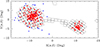 |
Fig. 1. Distribution of the T2Cs in the MCs. The red and blue filled circles show the stars with and without a match in the VMC database at the VSA (see text). The projection (zenithal equidistant) is centred at RA = 55.0 deg, Dec = −73.0 deg. The empty rectangles trace the footprint of the VMC survey. |
In the end, typically, we have 5−6 epochs in Y and J and 14−15 in Ks, as shown in Fig. 2. For some stars, the number of epochs is much larger. Indeed, if a variable falls into a region of overlap between two pawprints, the number of epochs is increased. We note that not all the T2Cs have VMC observations in all the filters: 315, 329 and 339 stars have photometry in the Y, J, and Ks bands, respectively. These samples represent 84%, 87% and 90% of the known T2Cs in the area surveyed by VMC. An example of a representative time series photometry in the J band is shown in Table 1. The full version of the table is available at the CDS.
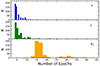 |
Fig. 2. Number of epochs for the T2C sample analysed in this work for the different VMC bands. |
Example of time-series photometry for the star OGLE-SMC-T2CEP-46 in the J band.
3. Data analysis
The time series light curves for the targets T2Cs were folded in phase using the periods and epoch of maximum from the literature (OGLE IV survey and Gaia mission DR3). The example light curves for the different T2C sub-classes are shown in Fig. 3. The following subsections define the procedure to determine our targets’ intensity-averaged magnitudes in each band. We followed the same methodology already adopted in our previous works, consisting of the use of templates to fit sparsely sampled light curves (see Ripepi et al. 2016, 2017, 2022a).
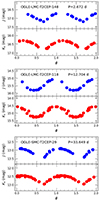 |
Fig. 3. Examples of light curves for different variability types. From top to bottom: BLHer, WVir, and RVTau, respectively. Both J and Ks bands data are shown. |
3.1. Template derivation
The first step of creating templates was to choose the best light curves among our sample of stars. For this purpose, we selected a subsample of stars with an adequate number of epochs (> 10) to ensure a good probability of having well-sampled light curves. As shown in Fig. 2, this first selection reduced significantly the number of objects to be considered in Y and J, while several tens of stars are available in Ks.
Then, we proceeded with a visual inspection of the light curves, considering only those showing the least scatter and ensuring the entire period range spanned by the data. We also retained the variety of light curve shapes representing the four different T2C types investigated in this work (BLHer, WVir, pWVir, and RVTau).
Following previous works on templates of CCs in the VMC survey (i.e. Ripepi et al. 2022a), the template-fitting procedure is carried out in two subsequent stages: (i) fitting the light curve with a spline function, and (ii) using a Fourier truncated series with at least 10 terms to fit the continuous spline curve obtained in the previous step. This two-step procedure was very successful in avoiding numerical ringing in the light curve fitting due to the small number of epochs and large phase gaps.
The first step was carried out with a custom build Python code, which adopts the splrep function to fit smooth spline curves to the data. The best smoothing factors were found using visual inspection of each light curve. The fitting spline curves have been subsequently transformed into templates by subtracting their intensity-averaged mean magnitude and re-scaling the amplitude to unity.
The second step consisted of fitting these normalised templates with a truncated Fourier series with 10 terms to ensure a perfect correspondence of the analytical function to the spline curve. The fitting equation is:
 (1)
(1)
where N is the number of harmonics, A0 the average magnitude (which in our case is zero), ϕ is the phase (intended as the adimensional substitute of time, it is therefore an observational independent variable); while Ai and Φi are the unknown coefficients of the series, i.e. the amplitude and the phase of each term. In the end, each template was transformed into a series of Fourier coefficients which are available in Appendix A.
The final template sample, shown in Fig. 4, contains 16 models for the Y band, 15 for the J band, and 31 for the Ks band. For each band, the templates are further divided by star type (BLHer, WVir, pWvir, RVTau).
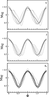 |
Fig. 4. Templates created in each band (labelled in the figures). |
3.2. Template fitting to the observed light curves
We used the procedure discussed in Ripepi et al. (2022a) to fit our light curves with the templates described above. Given that they have zero average and amplitude one, each template is adjusted to the real light curves by varying 3 parameters: (i) a magnitude shift δM; (ii) a scale factor, a, that increases or reduces the template amplitude to adapt it to that of the observed light curves; and (iii) a phase shift δϕ which takes into account possible differences in phase between templates and observed light curves. It is usual to impose that the maximum of the light curve is at phase 1 (or 0). To this aim, literature epochs of maximum from OGLE in the I band and from Gaia in the G band were used. The δϕ term also takes care of any small difference between the epoch of maximum in these two bands.
It is possible to obtain these three unknown numbers for each template by minimising the following χ2 function:
![Mathematical equation: $$ \begin{aligned} \chi ^2 = \sum _l^{N_{\rm pts}} \frac{[m_l - (a\times M_t(\phi _l + \delta \phi ) + \delta M)]^2}{\sigma _l^2}, \end{aligned} $$](/articles/aa/full_html/2024/05/aa48650-23/aa48650-23-eq2.gif) (2)
(2)
where Npts is the number of epochs, mi, ϕl and σl are the observed magnitudes, the corresponding phases, and the uncertainties on the magnitudes, respectively. Mt(ϕl) represents the template as a function of phase.
The fitting routine has an outlier rejection procedure, as the VMC light curves may show one or more bad measurements, due to various reasons (e.g. the star being hit by a cosmic ray or falling on a bad detector column, etc.). Outliers are detected by analysing the distribution of the residuals from the fit and spotting points outside the interval ±3.5 × DMAD, where DMAD is Double-Median Absolute Deviation4.
As we have fitted all the available templates to each star, we decide the best-fitting template using the so-called G parameter (introduced by Ripepi et al. 2016), which is defined as follows:
 (3)
(3)
where NU is the effective number of points used in the fit (after the rejection of outliers) and NT is the initial number of points (including outliers).
At the first visual analysis of the values of the amplitudes in the Y and J bands, we noticed a problem in the choice of the template for several objects for which the few epochs we have available in these bands were not evenly distributed along the light curve.
Indeed, as shown in Fig. 5 (top), objects with few observations not well spaced in phase, do not allow proper constraint on three parameters of the fit of Eq. (2). To overcome this problem, we introduced a parameter that evaluates the light curve’s sampling. This uniformity index was adopted according to the definition by Madore & Freedman (2005):
![Mathematical equation: $$ \begin{aligned} U_N^2 = \frac{N}{(N-1)} \left[1 - \sum ^N_{l=1} (\phi _{l+1}-\phi _l)^2\right], \end{aligned} $$](/articles/aa/full_html/2024/05/aa48650-23/aa48650-23-eq4.gif) (4)
(4)
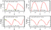 |
Fig. 5. Examples of fitting procedure. Top: light curves with incorrect templates. We note that for the RVTau variable, two points are out of the plot due to the very wrong amplitude. Bottom: light curves with the right template fitting for the same stars of the top panels. |
where N = NT and ϕl are defined as above (note that to calculate  , the epochs must be ordered in phase). Interpreted as a normalised variance, the
  statistic has a value of unity when the distribution of points is non-redundantly uniform over the light curve. After extensive visual inspection of large numbers of light curves, we verified that objects with
  < 0.6 have too scanty light curves to use Eq. (2) with three free parameters. Indeed, in these cases the sampling of the epochs prevented the algorithm from determining correctly the phase shift and the amplitude scaling. As a consequence (i) the phasing of the templates was very different from the expected ones based on the analysis of the OGLE I light curves; and (ii) the amplitude in Y or in J was larger than that in the I band, while it is expected the amplitudes decrease monotonically from optical to NIR bands. In all these cases, we decided to reduce the free parameters from three to two, by imposing a fixed amplitude scaling. To determine the proper amplitude scaling, we selected all the objects with
  > 0.9 and used their amplitudes in the I band (from the OGLE IV survey) to derive simple linear relations which are shown in Table 2. The adoption of this procedure fixes the problem as shown in Fig. 5 (bottom).
Coefficients of the linear relation between the amplitude in I band and in Y/J bands.
We used a Monte Carlo approach similar to Ripepi et al. (2016) to estimate the uncertainties on the fitted parameters. In brief, for each fitted source we generated 100 bootstrap simulations of the observed time series. The template fitting procedure was repeated for each mock time series and a statistical analysis of the obtained fitted parameters was performed. Our fitted parameters error estimate is given by the robust standard deviation (1.4826 × MAD) of the distributions obtained by the quoted bootstrap simulations.
The procedure outlined above allowed us to fit satisfactorily all the light curves using the best templates possible, eventually enabling the determination of accurate intensity-averaged magnitudes (and amplitudes) in all the bands. The final results for the whole sample of 339 targets are shown in Table 3, while examples of fitted light curves are shown in Fig. 6.
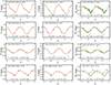 |
Fig. 6. Example BLHer, WVir, pWVir, and RVTau (from top to bottom row) light curves fitted in Y, J, Ks bands (left to right columns). Notes: green filled circles are the observations; the red solid line is the best template for the light curve; and black filled circles are the outlier data not used in the fit. |
VMC photometric parameters for all the 339 LMC and SMC T2Cs analysed in this work.
3.3. Reddening estimates for the target stars
To deal with the interstellar extinction, we took advantage of the recent accurate reddening maps published by Skowron et al. (2021). These maps have a varying spatial resolution, from 1.7 arcsec × 1.7 arcsec in the centre of the MCs to 27 arcsec × 27 arcsec in the peripheries, where there are fewer stars. They do not cover the entire extent of the MCs and were complemented by the same authors with the Schlegel et al. (1998, SFD hereafter) maps, which have a lower spatial resolution. As some of our targets were very distant from the MCs centres, the derived reddening values E(V − I) can be based either on Skowron et al. (2021) or the SFD maps.
The coefficients used to correct the magnitudes for the extinction were calculated according to Cardelli et al. (1989) assuming RV = A(V)/E(B − V) = 3.23 (Inno et al. 2013). For the Gaia bands we used the coefficients published by Casagrande & VandenBerg (2018). The adopted extinction coefficients, corresponding to the colour excess E(V − I), are reported in Table 4.
Extinction coefficient in different bands as a function of E(V − I).
3.4. Complementary optical data
We complemented the NIR VMC data with literature optical photometry to study the variation of PL relations with wavelength. In addition, we can also use Wesenheit magnitudes mixing optical and infrared bands. We added data in the V, I bands from the OGLE IV survey and in the G, GBP, GRP bands from the Gaia mission (Ripepi et al. 2023). The optical magnitudes from the literature were already calculated as intensity-averaged ones, so they do not need any transformation. All the optical data is listed in Table 5.
Optical photometric parameters for all the 339 LMC and SMC T2Cs analysed in this work.
The flag “SOURCE”, in Table 5, indicates whether the object was identified by OGLE IV or Gaia (as in Table 3). The flag “SOS” discerns the technique used to calculate the average magnitudes in the Gaia bands5: the value 0 indicates that the magnitudes are calculated with the standard technique adopted for all the stars (see e.g. Evans et al. 2018) and not specific for pulsating variables; the value 1 means that the magnitudes in the Gaia bands are calculated with the averaged-intensity technique after modelling the light curve (e.g. Clementini et al. 2016); the value 2 specifies that there are no magnitudes in the Gaia bands. Therefore, among the 318 T2Cs with OGLE IV identification, 316 have Gaia magnitudes: 85 and 231 with flag “SOS” = 0 and 1, respectively. The two missing stars have the flag “SOS” = 2.
We note that, while all the stars in the OGLE IV catalogue have the average I band magnitudes, not all have the V measurement. Moreover, the V, I data is completely missing for the stars originating from the Gaia catalogue and not present in OGLE IV. To recover the missing values in V, I bands, we used the photometric transformations between Johnson and Gaia bands provided by Pancino et al. (2022). They use high-order polynomials to obtain the V and I band photometry from G, GBP, GRP bands with uncertainties of 0.01 and 0.03 mag, respectively. The accuracy of transformations has been tested by Trentin et al. (2024), by comparing the V and I values from the Pancino et al. (2022) equations and those available in the literature for a sample of Galactic CCs. The calculated V magnitudes are accurate within 0.01 mag, as expected, while the I magnitudes result are too bright by 0.03 mag. As a consequence, we added to the transformed I magnitudes an offset of 0.03 mag.
The flag “VI”, in Table 5, marks the origin of the values of the V I magnitudes: the first part indicates the origin of the V value, the second of the I one. Usually, the stars identified by the OGLE survey have the flag “VI” equal to OGLE,OGLE. However, V magnitudes are missing for many T2Cs in the OGLE sample. In these cases, we adopted the Gaia magnitudes to estimate this quantity and the resulting “VI” flag is “P22;OGLE”. For the stars identified only by Gaia both V and I magnitudes are estimated from G, GBP, GRP data, so that we have “VI” flag equal to “P22;P22”. We note that the V I magnitudes estimated from the Gaia bands may have lower quality if the flag “SOS” is 0. In any case, the effect of the adoption of the standard averaged magnitudes are expected to be contained in a few per cent errors (see discussions on this point in Ripepi et al. 2022b; Gaia Collaboration 2023a).
4. Period–luminosity, period–wesenheit, and period–luminosity–colour relations
The multi-band photometry obtained as explained in the previous section has allowed us to calculate a significant number of PL, PLC and PW relations for the different classes of pulsating stars of interest for this work, separately for the LMC and SMC. In particular, we adopted different combinations of types: (i) BLHer; (ii) WVir; (iii) BLHer and WVir; (iv) BLHer, WVir, and pWVir; (v) BLHer, WVir, pWVir, and RVTau. Next, we describe briefly the sequence of procedures followed to calculate the above-mentioned relationships.
4.1. PL, PW and PLC derivation with the least trimmed squares algorithm
To determine the coefficients of the PL, PW and PLC relations, we fitted linear relations of the following types:
 (5)
(5)
 (6)
(6)
 (7)
(7)
where the observed quantities are the periods and the dereddened intensity averaged magnitudes. To carry out these linear fits in one or two dimensions, we adopted the Python code LTS (Least Trimmed Squares, Cappellari et al. 2013). This procedure is particularly robust with respect to the outlier removal because the clipping is carried out inside-out, contrary to the standard σ clipping.
4.2. Results for the PL, PW, and PLC relations
The PL relations were obtained in all the bands listed in the first column of Table 4. As for the wesenheit magnitudes, we calculated the PW relations for the five quantities defined in Table 6, where the coefficient of the colour term was obtained from the wavelength-dependent absorption values listed in the second column of Table 4. As for the Gaia bands, which have a wider bandwidth compared to Johnson–Cousins bands, we used the empirical Wesenheit function from Ripepi et al. (2019). As for the PLC, we considered the same magnitude–colour combinations which are at the base of the Wesenheit magnitudes shown in Table 6, where the colour coefficients are not fixed but free to vary.
An overview of the observational data at the base of all the PL relations to be derived in the LMC and SMC are reported in Figs. 7 and 8, respectively. Similarly, the left and right panels of Fig. 9 show the PW relations for T2Cs in the LMC and SMC, respectively. In all the figures, the different Cepheid types are highlighted with different colours. A visual inspection of these figures reveals several clear features, which will be later confirmed from a quantitative point of view:
-
In all the considered cases, the apparent dispersion of the data decreases from the optical to NIR bands. This is particularly evident in the LMC where the number of pulsators is much larger than in the SMC. The effect is also more evident among the PL relations compared to the PW ones, as these are in all cases much tighter than the former, with the exception of the J and Ks bands.
-
In the optical, the BLHer, WVir (and pWVir) and RVTau do not follow a unique linear PL relation. This is true also if we restrict the analysis to BLHer and WVir as is common in the literature. These types start following a unique PL relation for bands redder than I. According to Caputo et al. (2004), this is due to the different occupations of the IS in the optical bands for the T2Cs of different types.
-
In all the cases unique PW relations appear to be followed by all T2C types. This is due to two factors: (i) a better correction for the reddening, in the sense that the individual reddening corrections applied to the magnitudes at the base of the different PL relations are less effective than the use of the Wesenheit magnitudes which are reddening free by construction; (ii) the inclusion of the colour term in the construction of the Wesenheit magnitudes, that reduces significantly the difference in occupation of the IS which is likely the cause of the different behaviour of the different T2C subtypes in the PL diagrams.
-
In almost all the cases the RVTau stars show a larger dispersion compared to BLHer and WVir. This is due to possibly different origins of these stars, which, as discussed in the Sect. 1, could be a mixture of both old and intermediate-age stars. Also, BLHer variables are slightly more dispersed than WVir stars (excluding pWVir). This is likely due to the fainter magnitudes reached by these stars.
Taking into account these considerations, we have carried out the PL, PW and PLC fittings for each T2C type separately and then in different combinations in order to quantify the differences in the slopes between the different types or the possibility of combining the sub-samples.
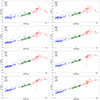 |
Fig. 7. Period–luminosity relations in all the considered bands from the optical to the NIR for T2Cs in the LMC. Blue, green, grey, and red filled circles represent BLHer, WVir, pWVir and RVTau pulsators, respectively. We note that the error bars are smaller than the dimensions of the dots. |
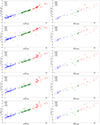 |
Fig. 9. Period–wesenheit relations in selected bands. Left panels: PW for T2Cs in the LMC. Right panels: same as left but for the SMC. The colours are the same as in Fig. 7. |
Examples of the PL and the PW fits are shown in Figs. 10 and 11 while all the figures showing the remaining fits can be found in Appendix C (Figs. C.1 and C.2 for the LMC and the SMC, respectively).
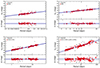 |
Fig. 10. Examples of PL fitting in the I band for different combinations of T2Cs in the LMC (see labels in the figures). The red and grey filled circles are the data used for the fit and the outliers, respectively. The solid black line is the best fit to the data, while the dashed blue lines show the ±1σ levels. For every figure in the top panel are plotted the fits while in the bottom panel the residuals of the fit. The colours are the same as above. The fits for the other bands are in the Appendix C. |
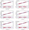 |
Fig. 11. Example best fits for BLHer and WVir in the LMC. From the top we show the PLKs, PWVI, PWVKs, PWJKs, PLCVKs, PLCG relations, respectively. The colours of dots and lines are the same as in Fig. 10. Additional fits are in the Appendix C. |
More in detail, Fig. 10 shows the PL relations in the I band for single and combined T2Cs types, while Fig. 11 displays selected tight PL and PW relations we obtain when combining BLHer and WVir types, only.
The results of the fit for all the considered cases and combination of types are reported in Tables 7 and 8, for the T2Cs in the LMC and SMC, respectively. These tables report the most interesting cases for the T2Cs, i.e. those without the more problematic RVTau pulsators. All the remaining cases are in Appendix C (Tables C.1 and C.2).
Coefficients of the PL, PLC, and PW relations for T2Cs in the LMC.
Inspecting these tables we find a confirmation of our previous qualitative assessments.
-
In the optical, PL relations calculated for BLHer and WVir have slopes which are different at several σ-levels. As we approach the J and Ks bands the slopes become consistent within less than 1σ.
-
The dispersion decreases going from optical to NIR bands. We will discuss this trend in more detail in the next Section.
-
The colour term, obtained from LTS plane fit, for the PLC relations in Ks, J − Ks and G, GBP − GRP is consistent, within 1σ, with the Wesenheit coefficient. This evidence demonstrates that the Wesenheit relations are not only reddening-free but also able to significantly account for the width of the IS.
For the reasons listed above, in the subsequent analyses, we will use the PL relations in the J and Ks bands and the PW relations in Ks, J − Ks, Ks, V − Ks and G, GBP − GRP.
5. Results
In this section, we exploit the PL, PW and PLC relations derived in this work and described in the previous Section. First, we discuss the dependence of the PL, PW and PLC coefficients on the wavelength. Secondly, we compare PL, PW and PLC relations with those in the literature.
5.1. Wavelength dependence of the PL, PW, and PLC coefficients
The extensive set of PL, PW and PLC calculations shown in Tables 7 and 8 (as well as Tables C.1 and C.2) allows us to investigate in detail how the slopes and the dispersions of these relations vary with the wavelength. This exercise permits us to choose the best relationships to use in further analysis and to verify a trend which is already known in the literature for the CCs: the slopes and the dispersions of the PL (PW/PLC) relations increase (in absolute value) and decrease at longer wavelengths, respectively. This anti-correlation was noted for the CCs by Madore & Freedman (1991) and explained on a physical basis by Madore & Freedman (2011). Indeed, they demonstrated that this feature is due to the different dependence of the surface brightness on the effective temperature at different wavelengths.
Figures 12 and 13 show the result of this investigation for the PL relations in a few selected cases for the LMC and SMC, respectively. Looking at the panels displaying the β (slope) and σ (dispersion) coefficients in each figure, the expected trends stand out, especially for the combination BLHer and WVir, in the LMC, which provides the tightest relations. The trends of slope and dispersion are slightly less evident for the SMC, where the significant depth along the line of sight (e.g. Ripepi et al. 2017) produces an additional dispersion due to the geometry of the system, which can be larger than the intrinsic width of the IS.
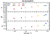 |
Fig. 12. Coefficients for the PL relations in optical and NIR bands for the LMC. α and σ are expressed in mag, β in mag dex−1. Only part of the figures are shown here for illustrative purposes, the remaining figures can be found in Appendix D. |
Similar trends are visible in the other PL relations calculated in this work (see Figs. D.1 and D.2). As for the PW relations (see Figs. D.1 and D.2), also in these cases, the general trend is the same as for the PLs but with a less clear behavior. This is because the inclusion of a colour term in the Wesenheit magnitudes tends to mitigate the effect of the width and the shape of the IS both in the optical and in the NIR bands. These results confirm and expand earlier findings by Matsunaga et al. (2006) and Ngeow et al. (2022).
5.2. Absolute calibration of PL and PW relations with the geometric distance of LMC
To compare our PL, PW and PLC with literature as well as to use them to calculate distances, it is mandatory to calibrate their zero points (intercepts) in absolute terms. To carry out this crucial procedure, we decided first to use the geometric distance of the LMC μLMC = 18.477 ± 0.026 mag as measured by Pietrzyński et al. (2019) based on a sample of eclipsing binaries (ECB).
The calibrated PL, PW, and PLC relations are listed in Table 9. As expected, the smallest dispersion is obtained for the NIR bands. The PW and PLC provide similar dispersion for the same combination of magnitudes and colours, confirming the goodness of the adopted reddening corrections. Furthermore, the analysis of the colour term coefficients (γ) of the derived PLC relations suggests that the optical PLC are less useful than the NIR counterparts. Indeed, the former show values of γ which are between ten and twenty times larger, thus small errors in the reddening produce large variations in the derived magnitudes. Particularly interesting is the PLC including V and Ks bands because as already found in our previous investigation (e.g. Ripepi et al. 2015), the γ coefficient is consistent within the errors with the colour term of the Wesenheit magnitude W(V, Ks). This means that this particular magnitude is not only reddening-free but also correct completely for the width of the IS.
Coefficients of the PL/PLC/PW relations for T2Cs in the LMC calibrated with D0, LMC = (18.477 ± 0.027) mag according to Pietrzyński et al. (2019).
5.3. Comparison with the literature
The relations in Table 9 (with absolute intercepts) and Table 7 (with relative intercepts) can now be compared to those available in the literature for the LMC and the GGCs.
Table 10 shows the comparison between a variety of PL, PW and PLC relation values from the literature (Matsunaga et al. 2006, 2011; Ripepi et al. 2015; Bhardwaj et al. 2017a) and our values. Figure 14 shows the comparison of our best relations with Matsunaga et al. (2009), Ripepi et al. (2015, 2019), Bhardwaj et al. (2017a), Wielgórski et al. (2022), Ngeow et al. (2022). Because the last three literature works were provided in the 2MASS photometric system, we adopted the conversion equations provided by González-Fernández et al. (2018) to convert from the 2MASS photometric system to the VISTA one: JVISTA = J2MASS − 0.0031(J − Ks)2MASS;  .
.
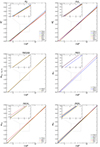 |
Fig. 14. Comparison of the best PL and PW relations of this work, labelled “TW23”, with previous works: Matsunaga et al. (2009, “MA09”), Ripepi et al. (2015, “RI15”), Ripepi et al. (2019, “RI19”), Bhardwaj et al. (2017a, “c”), Wielgórski et al. (2022, “WI22”), Ngeow et al. (2022, “NG22”). The inserts show a zoom-in of regions where there is high overlap between the different relations. |
Comparison among present PL and PW relations for T2Cs in the LMC and the literature values.
An inspection of the tables allows us to reach several considerations:
-
For each T2C sample and filter combination, our PL relations have been derived with the largest sample of stars and the resulting errors in the relation coefficients are the smallest compared to any literature work, especially in the NIR bands (see Table 10).
-
The coefficients of the BLHer PL relations (Table 10) in the J band are in agreement within 1σ with Bhardwaj et al. (2017a), within 1.5σ with Matsunaga et al. (2011, LMC) and within 2σ with Matsunaga et al. (2006, GGCs). In the Ks band, they agree within 1.5σ with Matsunaga et al. (2006, GGCs) and within 2σ with the others.
-
The coefficients of the WVir PL relations in J agree within 1σ with Bhardwaj et al. (2017a) and Matsunaga et al. (2011, LMC), disagree with Matsunaga et al. (2006, GGCs), while in the Ks band they are in agreement within 1σ only with Matsunaga et al. (2006, GGCs). All these discrepancies can be tentatively explained with the rather large uncertainties introduced in the fitting procedure by the short period range adopted when analysing WVir (and BLHer) separately. Indeed, when the two subtypes are used together, the agreement between the different works improves significantly (see below).
-
The coefficients of the PLs calculated using both BLHer and WVir in the J band agree within 1σ with Bhardwaj et al. (2017a), Ripepi et al. (2015) and Matsunaga et al. (2006), within 2σ with Matsunaga et al. (2011). In the Ks band, the agreement is generally worse, as in the previous cases, indeed the PL coefficients agree within 2σ with all the literature works, except Bhardwaj et al. (2017a) which is more discrepant.
-
Concerning the coefficients of the Wesenheit relations, there is a very good agreement with previous VMC results (Ripepi et al. 2015) while there is a large disagreement with Bhardwaj et al. (2017a). These differences could be due to Ks band photometry in Bhardwaj et al. (2017a), which was approaching the faint limit for the shortest-period BL Her stars.
-
The PLC values can only be compared with the previous VMC work (Ripepi et al. 2015) as shown in Table 11. The agreement is very good, especially in V and Ks, but with improved uncertainties in this work, owing to the larger sample.
-
In the SMC, the coefficients of our T2C PL and PW relations listed in Table 12 agree all within 1−2σ with Matsunaga et al. (2011) and Iwanek et al. (2018) (for the optical PWVI Wesenheit magnitude).
-
The PL slopes (β coefficients) for the LMC and the SMC agree within 1σ from the G to the Ks band, with the exception of GBP, which agrees within 2σ (see Tables 7 and 8).
-
The PWVKs and the PWJKs slopes (β coefficients) for the LMC and the SMC agree within 1σ, while the slopes of the others PW agree within 2σ.
Overall, the comparison with the literature shows good agreement, as for almost all the relations we find coefficients of PL, PW and PLC in agreement within better than 2σ for both the LMC and SMC. At the same time, in almost all cases, our data improves both the precision and the accuracy with respect to the literature, owing to larger samples, better light curve coverage, and deeper photometry guaranteed by the VMC survey.
Comparison of the present results with literature values for the PLC relations.
6. Applications
After having calibrated our best relationships by assuming the LMC distance, we derive the distances of selected GGCs hosting T2C variables and of selected field T2C stars having good multi-band photometry and Gaia parallaxes.
6.1. The distance to the GGCs with T2Cs PL and PW relations calibrated with the LMC geometric distance
To test the PL and PW relationships calibrated with the LMC geometric distance, we applied them to GGCs hosting T2Cs. Indeed, GGC distances can be derived from a variety of methods and are usually considered accurate (see Baumgardt & Vasiliev 2021, and references therein). To this aim, we collected a sample of 46 T2Cs belonging to 22 GGCs, taking from the literature only stars whose mean magnitudes were calculated as in our work (i.e. as intensity-averaged magnitudes and periods, see Bhardwaj et al. 2017b, 2021; Braga et al. 2020). We adopted distances (to compare with) from Ngeow et al. (2022), Baumgardt & Vasiliev (2021) and reddenings from Harris (2010). The Gaia photometry was missing in the quoted publications so we added it from the Gaia DR3 catalogue (e.g. Ripepi et al. 2023, see Table E.1).
To obtain the distance modulus (μ) of the GGC, we inserted the observed periods of the hosted T2Cs in our absolute PL and PW relations, obtaining the absolute magnitudes of these stars, which, combined with the apparent ones, provide the distances. When more than one pulsator was present in one GGC, the individual distances were averaged. The comparison between the μ calculated with our relations and those compiled by Ngeow et al. (2022), largely based on the work by Baumgardt & Vasiliev (2021), are shown in Fig. 15. As the sense of the difference in the lower panels is always literature – this work, it is clear that the literature distances are systematically larger. The first two columns of Table 13 quantify these differences. The largest discrepancy is obtained when the PL in the J band is used, while the minimum is found using PW relations, especially in the NIR bands, which also provide the smallest dispersion. The large difference between results based on the NIR PL and the PW relations is not easy to explain. We can hypothesise a not-perfectly homogeneous J, Ks photometry for GGCs data which is mitigated when using Wesenheit magnitudes. In any case, if we take the results for the PW relations as a reference, we have that the distance scale of GGCs is overestimated up to about 0.1 mag, assuming that the distance of the LMC is that provided by Pietrzyński et al. (2019). This supposition can imply a potential error as the spatial distribution of the late-type ECBs adopted by Pietrzyński et al. (2019) may differ from that spanned by the T2Cs in our sample. This occurrence could account for at least part of the observed shorter distances of the GGCs found in this section.
Median and σ for each GGC distance modulus difference (Δ) between Baumgardt & Vasiliev (2021) and this work (see Figs. 15, 17, and 18).
6.2. Absolute calibration of the T2Cs PL and PW relations using Gaia parallaxes
Given the unexpected result reported in the previous section, we decided to calibrate differently the zero points of the T2Cs PL and PW relations. Specifically, we adopt a sample of field Galactic T2Cs having optical photometry and parallax from Gaia DR3, while for a small sub-sample, we also used the NIR data published by Wielgórski et al. (2022). Given the small size of the latter sample, we decided to fix the slopes of the PL and PW relations to those of the LMC, which has been derived using a much larger number of pulsators. Before proceeding, we verified that the slope of the LMC adapts well to the Galactic data, as shown in Fig. 16, where we plotted the period–absolute WG, GBP − GRP6 relation for a sample of Galactic T2Cs having relative errors on the parallaxes better than 20% and overlapping the similar relation obtained for the LMC pulsators (with the zero point calculated from the LMC distance by Pietrzyński et al. 2019). The slope obtained in LMC perfectly describes the distribution of the galactic T2Cs at least in the Gaia Wesenheit.
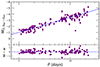 |
Fig. 16. Period vs. absolute Wesenheit magnitude in the Gaia bands (W(G, GBP − GRP) for a sample of Galactic T2Cs selected for having a relative error on the parallax of less than 20% (solid circles). The solid line has a slope calculated for the LMC sample and a zero point calculated using the geometric distance to the same galaxy (Pietrzyński et al. 2019). |
Having safely fixed the slopes of the different PL and PW relations to those of the LMC, we proceed to calculate the absolute zero points. To this aim, we cannot just invert the Gaia parallaxes to obtain the Galactic T2Cs distances lest to lose the statistical properties of parallaxes’ errors (e.g. Luri et al. 2018). Instead, we adopted two quantities, namely the photometric parallax (Feast & Whitelock 1997) and the astrometric-based luminosity (ABL, e.g. Arenou & Luri 1999) to carry out the calculations, which are described in detail in Appendix F.
The results of this procedure are shown in Table 14 which can be compared with Table 9, listing the results obtained from the use of the geometric distance to the LMC. To ease the comparison, we used the absolute zero points (i.e. the values of α) and the relative ones (Table 7) to directly calculate the distance modulus of the LMC and the SMC for the different PL and PW relations. These values and the relative errors are listed in the last part of Table 14.
Coefficients of the PL and PW relations for T2Cs with slope calculated in the LMC and zero point calibrated with Galactic T2Cs through photometric parallaxes (top) and ABL (bottom).
6.2.1. The LMC distance
The LMC distances obtained with the photometric parallax are systematically longer by 0.04−0.06 mag than the geometric value of Pietrzyński et al. (2019), except the result based on the PW relation in the Gaia bands, but consistent with it within 1σ. The LMC distances calculated through the ABL procedure are systematically larger than those obtained from the photometric parallax, with the largest deviation (0.04 mag) detected in the W(J, Ks) magnitude.
In general, the μLMC derived through the photometric parallax technique are in better agreement with the geometric μ (Pietrzyński et al. 2019) than those derived through the ABL. In any case, the PL and PW relations calibrated using the Gaia parallaxes of Galactic T2Cs provide larger μ by 0.05−0.06 mag on average than the (Pietrzyński et al. 2019) value.
This difference may be caused by the adopted Lindegren et al. (2021) individual zero point offsets which tend to over-correct the parallaxes and that require a counter-correction (see Groenewegen 2021; Riess et al. 2021; Ripepi et al. 2021, for discussions and references on this subject). To test this possibility, we adopted two typical values of the counter-correction among the many available in the literature: −14 μas (Riess et al. 2021) and −22 μas (Molinaro et al. 2023). However, the adoption of these offsets on the parallaxes has the effect of increasing the discrepancy, and therefore we retained the PL and PW relations with α values calculated adopting only the individual Lindegren et al. (2021) correction on parallaxes.
6.2.2. The SMC distance
Given the agreement among almost the totality of the slopes for the LMC and the SMC (see previous section), the zero points calculated using Galactic T2Cs can be used to estimate the distance modulus of the SMC (listed in the last columns of Table 14.
As for the LMC, the SMC distances calculated through the ABL procedure are systematically larger than those obtained from the photometric parallax.
In general, the μSMC derived through the photometric parallax technique are in better agreement with the geometric μ (Graczyk et al. 2020) than those derived through the ABL. The PL and PW relations calibrated using the Gaia parallaxes of Galactic T2Cs provide larger μ by 0.05−0.06 mag on average than the Graczyk et al. (2020) value (18.977 ± 0.016 ± 0.028 mag).
This result means that the ECB and T2C methods give approximately the same distance offset (0.5 mag) between the two clouds. This occurrence suggests that the method is solid and that the depth effects in the SMC are not a significant issue.
6.3. The distance of the GGCs based on absolute calibration with Gaia parallaxes
The relations of Table 14 can also be used to derive a new estimate of the distances of the GGCs, working with the same data set as in Sect. 6.1. Using the same formalism as in the first column of Table 13, we obtain the μ difference shown in the remaining columns of Table 13 and in Figs. 17 and 18. We find again that the distances by Baumgardt & Vasiliev (2021) are longer by about 0.03−0.06 mag than ours, even if by a smaller amount, at least when using the PL relations.
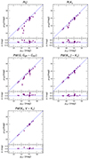 |
Fig. 17. Comparison between our distances based on photometric parallaxes and those of Baumgardt & Vasiliev (2021). |
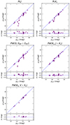 |
Fig. 18. Comparison between our distances based on ABL and those of Baumgardt & Vasiliev (2021). |
In analogy with the LMC distance estimation, we can also compare the GGCs distance moduli obtained both from the ABL and the photometric parallaxes procedures with the literature ones (i.e. Baumgardt & Vasiliev 2021). As expected, we find smaller differences with the GGCs distances calculated with the ABL than the photometric parallax case. In particular, the NIR Wesenheit magnitudes provide agreement within 1σ.
6.4. Comparison between GGC distances based on T2Cs and RRL stars
Several GGCs hosting T2Cs also host RRL variables (see also the Sect. 1). Given that RRL stars are noticeably good distance indicators, especially in the NIR regime, they can be used to obtain GGCs distances which are independent from those by Baumgardt & Vasiliev (2021). We can therefore compare the distances of the GGCs hosting both RRL and T2Cs and verify the compatibility of the distance scales associated with these two old population distance indicators.
To this purpose, we considered the work by Bhardwaj et al. (2023), who calculated the distances for a significant sample of GGCs using NIR PL and PW relations for RRL stars based on homogeneous photometry. In Table 15 we compare in the usual way the μ values obtained in different ways in this work (see the previous sections) for 7 GGCs hosting T2Cs and the corresponding values calculated with the RRL variables.
As in Table 13, but for the comparison with the GGC distances by Bhardwaj et al. (2023).
The resulting Δ values are similar to those shown in Table 13 when we compared our results with those of Baumgardt & Vasiliev (2021). However, the size of the discrepancy is smaller by a ∼0.01−0.02 mag. This is not surprising, as Bhardwaj et al. (2023) found that the RRL-based GGCs distances are smaller by about 0.015 mag than those provided by Baumgardt & Vasiliev (2021). In any case, if we use the PL and PW relations calibrated with the Gaia parallaxes the T2C and RRL distance scales agree better than 1−2σ if we consider the PW(J, Ks) and PW(V, Ks) relations, while we have 3σ difference in the other cases. The situation is worse if we calibrate our relationships with the geometric distance of the LMC. Indeed, in this case, the discrepancy is generally larger than 3σ of their quoted uncertainties.
7. Discussion and conclusions
In this study, we exploited Y, J, and Ks time-series photometry for a sample of more than 330 T2Cs located in the LMC and SMC in the context of the ESO public survey VISTA survey of the Magellanic Clouds system (VMC). We complemented the VMC data with optical data from the OGLE IV survey and the Gaia mission. From these surveys, we obtained the identification and positions of the pulsators, their periods, and their photometry in the V, I, G, GBP, GRP bands.
After selecting the best VMC time series, we built a set of light-curve templates for each T2C subtype. We used these templates to derive accurate intensity-averaged magnitudes (and amplitudes) for all the pulsators at our disposal through a sophisticated pipeline already developed in the context of previous VMC works dealing with CCs. This pipeline was further improved in the course of the present work by introducing a parameter that takes into account the sampling of the observed light curve, which enables a special treatment of the poorly sampled curves, allowing us to keep stars that would otherwise have been rejected.
The final Y, J, and Ks photometry obtained in this way complemented with the above-mentioned optical data, was used to build a large set of PL, PW, and PLC relations for a variety of T2C subtypes (BLHer, WVir, RVTau, and combinations). To this aim, we employed a Python-based robust algorithm, LTS, which embodies a sound outlier rejection procedure.
The multi-band PL relations produced during this work were used to systematically investigate the dependence of T2C relations – namely the slopes and the dispersion – on the adopted wavelength for the first time. Similarly to the case for CCs, our results show that, even for these older pulsators, the slope increases and the dispersion decreases as we move towards longer wavelengths.
Overall, there is good agreement with the literature, as for almost all the relations we find coefficients of the PL, PW and PLC relations in agreement to within less than 2σ for both the LMC and SMC. At the same time, in almost all cases, our data improve both precision and accuracy compared to previous studies, owing to larger samples, better light-curve sampling, and deeper photometry as guaranteed by the VMC survey (see Table 10).
The tightest relationships derived in this work, namely the PL in J and Ks bands, and all the PW relations in the LMC, all showing low dispersions, were calibrated by anchoring their absolute zero points (intercepts) to the geometric distance of the LMC, as accurately determined from a set of ECBs. These absolute relationships were used to derive the distances of a sample of 22 GGCs hosting T2Cs, finding that the most up-to-date literature distances (e.g. Baumgardt & Vasiliev 2021) are larger by some 0.10 mag with a 3σ significance. Therefore, the geometric distance of the LMC by Pietrzyński et al. (2019) appears to be in disagreement with the GGC distance scale.
Stimulated by this unexpected result, we calibrated the PL and PW relations independently from the LMC distance using a sample of Galactic field T2Cs for which accurate data in optical and NIR bands are available in the literature. To this aim, we adopted the slopes of the LMC (which are reasonably compatible with those of the MW and SMC) and calculated the zero points of the PL and PW relations using the Gaia EDR3 parallaxes.
Using these relations, we recalculated the distance of the LMC and SMC analysed before. As a result, we obtained a μLMC that is ∼0.06 mag longer on average than the geometric estimate provided by Pietrzyński et al. (2019), albeit in agreement within 1σ. This result is in agreement with previous investigations (Wielgórski et al. 2022). A similar result was obtained by Graczyk et al. (2020) for the SMC in comparison with the geometric distance of this galaxy. Concerning the GGCs, the μ obtained with the new calibration is still substantially shorter than those reported by Baumgardt & Vasiliev (2021), that is, by amounts of the order of 0.03−0.06 mag for the most precise PW relations with a typical significance of 1−2σ. A better agreement by 0.01−0.02 mag is obtained when we compare our results with the distances of the GGCs obtained from RRL variables only (Bhardwaj et al. 2023). This occurrence is particularly important, as one of the most important developments of this work is using of both RRL and T2C to calibrate the TRGB in an alternative route to calibrate H0.
It is not easy to interpret these conflicting results. One possibility is to invoke a significant effect of the metallicity – which we neglected in this paper – based on the theoretical and empirical results of Ripepi et al. (2015) and Ngeow et al. (2022, and references therein), who do not report a significant metallicity dependence of T2C PL and PW relations. However, even a significant metallicity effect seems insufficient to simultaneously reconcile the distances of the LMC (and SMC) and the GGCs, given the large range of abundances spanned by the latter. A more likely possible explanation is that the spatial distributions of the late-type ECBs adopted by Pietrzyński et al. (2019) and Graczyk et al. (2020) to derive the geometric distances of the LMC and the SMC differ significantly from those spanned by the T2Cs in our samples. This occurrence could account for at least part of the observed discrepancy.
The advent of large spectroscopic surveys such as those foreseen with WEAVE (WHT Enhanced Area Velocity Explorer)7 and 4MOST (4-m Multi-Object Spectroscopic Telescope)8, as well as the availability of more accurate parallaxes thanks to the future Gaia DR4, will certainly provide us with the information needed to draw firmer conclusions as to the distance scale of T2C and help us to understand the discrepant results we obtained in this work concerning the distances of the LMC and the GGC system.
The Wesenheit magnitudes are constructed to be reddening free by definition (Madore 1982).
The ESO archive (https://www.eso.org/qi/) contains all the information on the different data products of the VMC survey.
DMAD is calculated by treating the values smaller and larger than the median of the considered distribution separately.
SOS stands for Specific Object Studies (see e.g. Ripepi et al. 2023).
The absolute magnitudes were derived using G − 1.9 × (GBP − GRP)+5 × log(ϖ)−10, where ϖ is the Gaia EDR3 parallax corrected using the Lindegren et al. (2021) relations (see next sections).
Acknowledgments
We warmly thank our anonymous referee for their competent and helpful comments. We thank Mauricio Cruz Reyes for interesting and helpful discussion about GGCs distances. We thank Jacco Th. van Loon for helpful discussion on the manuscript. This research has made use of the SIMBAD database, operated at CDS, Strasbourg, France. This work has made use of data from the European Space Agency (ESA) mission Gaia (https://www.cosmos.esa.int/gaia), processed by the Gaia Data Processing and Analysis Consortium (DPAC, https://www.cosmos.esa.int/web/gaia/dpac/consortium). Funding for the DPAC has been provided by national institutions, in particular, the institutions participating in the Gaia Multilateral Agreement. This research was supported in part by the Australian Research Council Centre of Excellence for All Sky Astrophysics in 3 Dimensions (ASTRO 3D), through project number CE170100013.
References
- Alcock, C., Allsman, R. A., Alves, D. R., et al. 1998, ApJ, 492, 190 [NASA ADS] [CrossRef] [Google Scholar]
- Arenou, F., & Luri, X. 1999, ASP Conf. Ser., 167, 13 [Google Scholar]
- Baumgardt, H., & Vasiliev, E. 2021, MNRAS, 505, 5957 [NASA ADS] [CrossRef] [Google Scholar]
- Beaton, R. L., Freedman, W. L., Madore, B. F., et al. 2016, ApJ, 832, 210 [Google Scholar]
- Bhardwaj, A. 2020, JApA, 41, 23 [NASA ADS] [Google Scholar]
- Bhardwaj, A. 2022, Universe, 8, 122 [NASA ADS] [CrossRef] [Google Scholar]
- Bhardwaj, A., Macri, L. M., Rejkuba, M., et al. 2017a, AJ, 153, 154 [NASA ADS] [CrossRef] [Google Scholar]
- Bhardwaj, A., Rejkuba, M., Minniti, D., et al. 2017b, A&A, 605, A100 [NASA ADS] [CrossRef] [EDP Sciences] [Google Scholar]
- Bhardwaj, A., Rejkuba, M., de Grijs, R., et al. 2021, ApJ, 909, 200 [NASA ADS] [CrossRef] [Google Scholar]
- Bhardwaj, A., Marconi, M., Rejkuba, M., et al. 2023, ApJ, 944, L51 [NASA ADS] [CrossRef] [Google Scholar]
- Bono, G., Braga, V., Fiorentino, G., et al. 2020, A&A, 644, A96 [NASA ADS] [CrossRef] [EDP Sciences] [Google Scholar]
- Braga, V. F., Bhardwaj, A., Contreras Ramos, R., et al. 2018, A&A, 619, A51 [NASA ADS] [CrossRef] [EDP Sciences] [Google Scholar]
- Braga, V., Bono, G., Fiorentino, G., et al. 2020, A&A, 644, A95 [NASA ADS] [CrossRef] [EDP Sciences] [Google Scholar]
- Cappellari, M., Scott, N., Alatalo, K., et al. 2013, MNRAS, 432, 1709 [Google Scholar]
- Caputo, F., Castellani, V., Degl’Innocenti, S., Fiorentino, G., & Marconi, M. 2004, A&A, 424, 927 [NASA ADS] [CrossRef] [EDP Sciences] [Google Scholar]
- Cardelli, J. A., Clayton, G. C., & Mathis, J. S. 1989, ApJ, 345, 245 [Google Scholar]
- Casagrande, L., & VandenBerg, D. A. 2018, MNRAS, 479, L102 [NASA ADS] [CrossRef] [Google Scholar]
- Cioni, M.-R., Clementini, G., Girardi, L., et al. 2011, A&A, 527, A116 [CrossRef] [EDP Sciences] [Google Scholar]
- Clementini, G., Ripepi, V., Leccia, S., et al. 2016, A&A, 595, A133 [NASA ADS] [CrossRef] [EDP Sciences] [Google Scholar]
- Clementini, G., Ripepi, V., Molinaro, R., et al. 2019, A&A, 622, A60 [NASA ADS] [CrossRef] [EDP Sciences] [Google Scholar]
- Clementini, G., Ripepi, V., Garofalo, A., et al. 2023, A&A, 674, A18 [NASA ADS] [CrossRef] [EDP Sciences] [Google Scholar]
- Cross, N. J. G., Collins, R. S., Mann, R. G., et al. 2012, A&A, 548, A119 [NASA ADS] [CrossRef] [EDP Sciences] [Google Scholar]
- Dalton, G. B., Caldwell, M., Ward, A. K., et al. 2006, in Society of Photo-Optical Instrumentation Engineers (SPIE) Conference Series, eds. I. S. McLean, & M. Iye, 6269, 62690X [NASA ADS] [Google Scholar]
- Das, S., Kanbur, S. M., Smolec, R., et al. 2021, MNRAS, 501, 875 [Google Scholar]
- Di Criscienzo, M., Caputo, F., Marconi, M., & Cassisi, S. 2007, A&A, 471, 893 [NASA ADS] [CrossRef] [EDP Sciences] [Google Scholar]
- Emerson, J., McPherson, A., & Sutherland, W. 2006, The Messenger, 126, 41 [NASA ADS] [Google Scholar]
- Evans, D. W., Riello, M., De Angeli, F., et al. 2018, A&A, 616, A4 [NASA ADS] [CrossRef] [EDP Sciences] [Google Scholar]
- Feast, M., & Whitelock, P. 1997, MNRAS, 291, 683 [NASA ADS] [CrossRef] [Google Scholar]
- Feast, M. W., Laney, C. D., Kinman, T. D., Van Leeuwen, F., & Whitelock, P. A. 2008, MNRAS, 386, 2115 [NASA ADS] [CrossRef] [Google Scholar]
- Freedman, W. L. 2021, ApJ, 919, 16 [NASA ADS] [CrossRef] [Google Scholar]
- Gaia Collaboration (Prusti, T., et al.) 2016, A&A, 595, A1 [NASA ADS] [CrossRef] [EDP Sciences] [Google Scholar]
- Gaia Collaboration (Drimmel, R., et al.) 2023a, A&A, 674, A37 [CrossRef] [EDP Sciences] [Google Scholar]
- Gaia Collaboration (Vallenari, A., et al.) 2023b, A&A, 674, A1 [NASA ADS] [CrossRef] [EDP Sciences] [Google Scholar]
- Gingold, R. A. 1976, ApJ, 204, 116 [NASA ADS] [CrossRef] [Google Scholar]
- Gingold, R. A. 1985, Mem. Soc. Astron. It., 56, 169 [Google Scholar]
- González-Fernández, C., Hodgkin, S. T., Irwin, M. J., et al. 2018, MNRAS, 474, 5459 [Google Scholar]
- Graczyk, D., Pietrzyński, G., Thompson, I. B., et al. 2020, ApJ, 904, 13 [Google Scholar]
- Groenewegen, M. A. T. 2021, A&A, 654, A20 [NASA ADS] [CrossRef] [EDP Sciences] [Google Scholar]
- Groenewegen, M. A. T., & Jurkovic, M. I. 2017, A&A, 604, A29 [NASA ADS] [CrossRef] [EDP Sciences] [Google Scholar]
- Hamanowicz, A., Pietrukowicz, P., Udalski, A., et al. 2016, Acta Astron., 66, 197 [NASA ADS] [Google Scholar]
- Harris, W. E. 2010, arXiv e-prints [arXiv:1012.3224] [Google Scholar]
- Inno, L., Matsunaga, N., Bono, G., et al. 2013, ApJ, 764, 84 [Google Scholar]
- Irwin, M. J., Lewis, J., Hodgkin, S., et al. 2004, Proc. SPIE, 5493, 411 [Google Scholar]
- Iwanek, P., Soszyński, I., Skowron, D., et al. 2018, Acta Astron., 68, 213 [NASA ADS] [Google Scholar]
- Lindegren, L., Bastian, U., Biermann, M., et al. 2021, A&A, 649, A4 [EDP Sciences] [Google Scholar]
- Luri, X., Brown, A. G. A., Sarro, L. M., et al. 2018, A&A, 616, A9 [NASA ADS] [CrossRef] [EDP Sciences] [Google Scholar]
- Madore, B. 1982, ApJ, 253, 575 [NASA ADS] [CrossRef] [Google Scholar]
- Madore, B. F., & Freedman, W. L. 1991, PASP, 103, 933 [Google Scholar]
- Madore, B. F., & Freedman, W. L. 2005, ApJ, 630, 1054 [NASA ADS] [CrossRef] [Google Scholar]
- Madore, B. F., & Freedman, W. L. 2011, ApJ, 744, 132 [Google Scholar]
- Marconi, M., & Di Criscienzo, M. 2007, A&A, 467, 223 [EDP Sciences] [Google Scholar]
- Mathewson, D. S., Cleary, M. N., & Murray, J. D. 1974, in Galactic Radio Astronomy, eds. F. J. Kerr, & S. C. Simonson, 60, 617 [NASA ADS] [CrossRef] [Google Scholar]
- Matsunaga, N., Fukushi, H., Nakada, Y., et al. 2006, MNRAS, 370, 1979 [Google Scholar]
- Matsunaga, N., Feast, M. W., & Menzies, J. W. 2009, MNRAS, 397, 933 [NASA ADS] [CrossRef] [Google Scholar]
- Matsunaga, N., Feast, M. W., & Soszyński, I. 2011, MNRAS, 413, 223 [Google Scholar]
- Molinaro, R., Ripepi, V., Marconi, M., et al. 2023, MNRAS, 520, 4154 [NASA ADS] [CrossRef] [Google Scholar]
- Moretti, M. I., Clementini, G., Muraveva, T., et al. 2014, MNRAS, 437, 2702 [Google Scholar]
- Ngeow, C.-C., Bhardwaj, A., Henderson, J.-Y., et al. 2022, AJ, 164, 154 [NASA ADS] [CrossRef] [Google Scholar]
- Pancino, E., Marrese, P. M., Marinoni, S., et al. 2022, A&A, 664, A109 [NASA ADS] [CrossRef] [EDP Sciences] [Google Scholar]
- Pietrzyński, G., Graczyk, D., Gallenne, A., et al. 2019, Nature, 567, 200 [Google Scholar]
- Planck Collaboration VI. 2020, A&A, 641, A6 [NASA ADS] [CrossRef] [EDP Sciences] [Google Scholar]
- Riess, A. G., Casertano, S., Yuan, W., et al. 2021, ApJ, 908, L6 [NASA ADS] [CrossRef] [Google Scholar]
- Riess, A. G., Yuan, W., Macri, L. M., et al. 2022, ApJ, 934, L7 [NASA ADS] [CrossRef] [Google Scholar]
- Ripepi, V., Moretti, M. I., Marconi, M., et al. 2012, MNRAS, 424, 1807 [Google Scholar]
- Ripepi, V., Moretti, M. I., Marconi, M., et al. 2015, MNRAS, 446, 3034 [NASA ADS] [CrossRef] [Google Scholar]
- Ripepi, V., Marconi, M., Moretti, M. I., et al. 2016, ApJS, 224, 21 [Google Scholar]
- Ripepi, V., Cioni, M.-R. L., Moretti, M. I., et al. 2017, MNRAS, 472, 808 [Google Scholar]
- Ripepi, V., Molinaro, R., Musella, I., et al. 2019, A&A, 625, A14 [NASA ADS] [CrossRef] [EDP Sciences] [Google Scholar]
- Ripepi, V., Catanzaro, G., Molinaro, R., et al. 2021, MNRAS, 508, 4047 [NASA ADS] [CrossRef] [Google Scholar]
- Ripepi, V., Chemin, L., Molinaro, R., et al. 2022a, MNRAS, 512, 563 [NASA ADS] [CrossRef] [Google Scholar]
- Ripepi, V., Catanzaro, G., Clementini, G., et al. 2022b, A&A, 659, A167 [NASA ADS] [CrossRef] [EDP Sciences] [Google Scholar]
- Ripepi, V., Clementini, G., Molinaro, R., et al. 2023, A&A, 674, A17 [NASA ADS] [CrossRef] [EDP Sciences] [Google Scholar]
- Schlegel, D. J., Finkbeiner, D. P., & Davis, M. 1998, ApJ, 500, 525 [Google Scholar]
- Skowron, D., Skowron, J., Udalski, A., et al. 2021, ApJS, 252, 23 [NASA ADS] [CrossRef] [Google Scholar]
- Soszyński, I., Udalski, A., Szymański, M. K., et al. 2008, Acta Astron., 58, 293 [NASA ADS] [Google Scholar]
- Soszyński, I., Udalski, A., Szymański, M. K., et al. 2018, Acta Astron., 68, 89 [NASA ADS] [Google Scholar]
- Trentin, E., Ripepi, V., Molinaro, R., et al. 2024, A&A, 681, A65 [NASA ADS] [CrossRef] [EDP Sciences] [Google Scholar]
- Wallerstein, G. 2002, PASP, 114, 689 [Google Scholar]
- Wielgórski, P., Pietrzyński, G., Pilecki, B., et al. 2022, ApJ, 927, 89 [CrossRef] [Google Scholar]
Appendix A: Template fitting
The tables in this Appendix list the coefficients of the templates adopted to fit the observed light curves in the Y, J, and Ks bands.
Fourier parameters of the light curves templates in Y band.
Same as Table A.1 but in J band.
Same as Table A.1 but in Ks band.
Appendix B: Example light-curve fits with templates
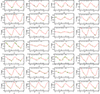 |
Fig. B.1. Examples of fitted templates for T2C light curves in Y. |
Appendix C: Additional PL, PW and PLC relations in the LMC and SMC
In this section, we show the PL, PW and PLC fitting to the data for a variety of magnitudes, colours and Wesenheit magnitudes, as well as the parameters from the fitting.
C.1. Figures
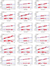 |
Fig. C.1. Relation fitting in different bands for a variety of T2C class combinations in the LMC. |
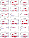 |
Fig. C.1. continued. |
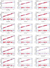 |
Fig. C.1. continued. |
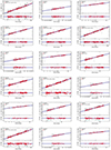 |
Fig. C.1. continued. |
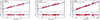 |
Fig. C.1. continued. |
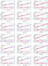 |
Fig. C.2. continued. |
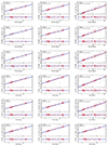 |
Fig. C.2. continued. |
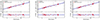 |
Fig. C.2. continued. |
C.2. Tables
Continued from Table 7.
Continued from Table 8.
Appendix D: Additional wavelength dependence of PL, PW and PLC relations
In this section, we show the wavelength dependence of the coefficients of several PL, PW and PLC relations. These figures complete the results shown in Fig. 12 and 13.
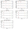 |
Fig. D.1. Coefficients for the PL snd PW relations in optical and NIR bands for LMC. α and σ are expressed in mag, β in mag/dex. |
Appendix E: Sample of T2Cs hosted in the GGs
Optical and NIR photometric parameters for the 46 GGCs T2Cs analysed in this work.
Appendix F: Calibration with Galactic T2Cs parallaxes
F.1. Calibration with the Photometric parallax
We first defined the photometric parallax (in mas):
 (F.1)
(F.1)
where m is the apparent magnitude (or apparent Wesenheit magnitude); M is the absolute magnitude (or absolute Wesenheit magnitude), defined as:
 (F.2)
(F.2)
where βLMC are the slopes obtained for the LMC and listed in Table 7. Given the scarcity of the sample of stars with known metallicity (Wielgórski et al. 2022), we did not include a metallicity term in the PL and PW relations. However, this is not a major issue, as several papers reported a negligible metallicity dependence of these relations for the T2Cs (Matsunaga et al. 2009; Ripepi et al. 2015; Ngeow et al. 2022) at odds with Wielgórski et al. (2022) results, which are, however, based on a very small sample of T2Cs with metallicity measurement and must be confirmed.
The value of α is thus obtained by minimising the following χ2 expression:
 (F.3)
(F.3)
where ϖEDR3 are the parallaxes from Gaia EDR3 corrected individually with the recipe provided by Lindegren et al. (2021). The fitting procedure is described in detail by Ripepi et al. (2022b) and is not repeated here. The interested reader is referred to the quoted paper.
F.2. Calibration with the ABL
In addition to the photometric parallax method, we also used the ABL with a different fitting technique to estimate the zero points of T2C PL snd PW. By using two different methods, we can compare the obtained results. The ABL is defined as:
 (F.4)
(F.4)
where, as above, W and w are the absolute and apparent Wesenheit magnitudes and ϖ is the parallax, while, as in the previous case, the slope (βLMC) is fixed to that of the LMC. The χ2 expression in this case is:
 (F.5)
(F.5)
where the different quantities have the same meaning as in Eq. F.4 and σ includes all the errors. The results for the unknown α are listed in the bottom part of Table 14.
All Tables
Coefficients of the linear relation between the amplitude in I band and in Y/J bands.
VMC photometric parameters for all the 339 LMC and SMC T2Cs analysed in this work.
Optical photometric parameters for all the 339 LMC and SMC T2Cs analysed in this work.
Coefficients of the PL/PLC/PW relations for T2Cs in the LMC calibrated with D0, LMC = (18.477 ± 0.027) mag according to Pietrzyński et al. (2019).
Comparison among present PL and PW relations for T2Cs in the LMC and the literature values.
Comparison of the present results with literature values for the PLC relations.
Median and σ for each GGC distance modulus difference (Δ) between Baumgardt & Vasiliev (2021) and this work (see Figs. 15, 17, and 18).
Coefficients of the PL and PW relations for T2Cs with slope calculated in the LMC and zero point calibrated with Galactic T2Cs through photometric parallaxes (top) and ABL (bottom).
As in Table 13, but for the comparison with the GGC distances by Bhardwaj et al. (2023).
Optical and NIR photometric parameters for the 46 GGCs T2Cs analysed in this work.
All Figures
|
Fig. 1. Distribution of the T2Cs in the MCs. The red and blue filled circles show the stars with and without a match in the VMC database at the VSA (see text). The projection (zenithal equidistant) is centred at RA = 55.0 deg, Dec = −73.0 deg. The empty rectangles trace the footprint of the VMC survey. |
| In the text | |
|
Fig. 2. Number of epochs for the T2C sample analysed in this work for the different VMC bands. |
| In the text | |
|
Fig. 3. Examples of light curves for different variability types. From top to bottom: BLHer, WVir, and RVTau, respectively. Both J and Ks bands data are shown. |
| In the text | |
|
Fig. 4. Templates created in each band (labelled in the figures). |
| In the text | |
|
Fig. 5. Examples of fitting procedure. Top: light curves with incorrect templates. We note that for the RVTau variable, two points are out of the plot due to the very wrong amplitude. Bottom: light curves with the right template fitting for the same stars of the top panels. |
| In the text | |
|
Fig. 6. Example BLHer, WVir, pWVir, and RVTau (from top to bottom row) light curves fitted in Y, J, Ks bands (left to right columns). Notes: green filled circles are the observations; the red solid line is the best template for the light curve; and black filled circles are the outlier data not used in the fit. |
| In the text | |
|
Fig. 7. Period–luminosity relations in all the considered bands from the optical to the NIR for T2Cs in the LMC. Blue, green, grey, and red filled circles represent BLHer, WVir, pWVir and RVTau pulsators, respectively. We note that the error bars are smaller than the dimensions of the dots. |
| In the text | |
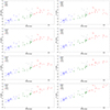 |
Fig. 8. Same as Fig. 7, but for the SMC. |
| In the text | |
|
Fig. 9. Period–wesenheit relations in selected bands. Left panels: PW for T2Cs in the LMC. Right panels: same as left but for the SMC. The colours are the same as in Fig. 7. |
| In the text | |
|
Fig. 10. Examples of PL fitting in the I band for different combinations of T2Cs in the LMC (see labels in the figures). The red and grey filled circles are the data used for the fit and the outliers, respectively. The solid black line is the best fit to the data, while the dashed blue lines show the ±1σ levels. For every figure in the top panel are plotted the fits while in the bottom panel the residuals of the fit. The colours are the same as above. The fits for the other bands are in the Appendix C. |
| In the text | |
|
Fig. 11. Example best fits for BLHer and WVir in the LMC. From the top we show the PLKs, PWVI, PWVKs, PWJKs, PLCVKs, PLCG relations, respectively. The colours of dots and lines are the same as in Fig. 10. Additional fits are in the Appendix C. |
| In the text | |
|
Fig. 12. Coefficients for the PL relations in optical and NIR bands for the LMC. α and σ are expressed in mag, β in mag dex−1. Only part of the figures are shown here for illustrative purposes, the remaining figures can be found in Appendix D. |
| In the text | |
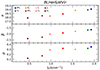 |
Fig. 13. As in Fig. 12, but for the SMC. |
| In the text | |
|
Fig. 14. Comparison of the best PL and PW relations of this work, labelled “TW23”, with previous works: Matsunaga et al. (2009, “MA09”), Ripepi et al. (2015, “RI15”), Ripepi et al. (2019, “RI19”), Bhardwaj et al. (2017a, “c”), Wielgórski et al. (2022, “WI22”), Ngeow et al. (2022, “NG22”). The inserts show a zoom-in of regions where there is high overlap between the different relations. |
| In the text | |
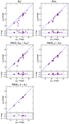 |
Fig. 15. Comparison between our distances and those by Baumgardt & Vasiliev (2021). |
| In the text | |
|
Fig. 16. Period vs. absolute Wesenheit magnitude in the Gaia bands (W(G, GBP − GRP) for a sample of Galactic T2Cs selected for having a relative error on the parallax of less than 20% (solid circles). The solid line has a slope calculated for the LMC sample and a zero point calculated using the geometric distance to the same galaxy (Pietrzyński et al. 2019). |
| In the text | |
|
Fig. 17. Comparison between our distances based on photometric parallaxes and those of Baumgardt & Vasiliev (2021). |
| In the text | |
|
Fig. 18. Comparison between our distances based on ABL and those of Baumgardt & Vasiliev (2021). |
| In the text | |
|
Fig. B.1. Examples of fitted templates for T2C light curves in Y. |
| In the text | |
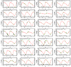 |
Fig. B.2. Same as Fig. B.1, but in J band. |
| In the text | |
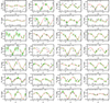 |
Fig. B.3. Same as Fig. B.1, but in Ks band. |
| In the text | |
|
Fig. C.1. Relation fitting in different bands for a variety of T2C class combinations in the LMC. |
| In the text | |
|
Fig. C.1. continued. |
| In the text | |
|
Fig. C.1. continued. |
| In the text | |
|
Fig. C.1. continued. |
| In the text | |
|
Fig. C.1. continued. |
| In the text | |
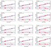 |
Fig. C.2. Same as Fig. C.1, but for SMC. |
| In the text | |
|
Fig. C.2. continued. |
| In the text | |
|
Fig. C.2. continued. |
| In the text | |
|
Fig. C.2. continued. |
| In the text | |
|
Fig. D.1. Coefficients for the PL snd PW relations in optical and NIR bands for LMC. α and σ are expressed in mag, β in mag/dex. |
| In the text | |
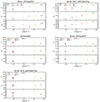 |
Fig. D.2. Same as Fig. D.1 but for the SMC. |
| In the text | |
Current usage metrics show cumulative count of Article Views (full-text article views including HTML views, PDF and ePub downloads, according to the available data) and Abstracts Views on Vision4Press platform.
Data correspond to usage on the plateform after 2015. The current usage metrics is available 48-96 hours after online publication and is updated daily on week days.
Initial download of the metrics may take a while.