| Issue |
A&A
Volume 699, July 2025
|
|
|---|---|---|
| Article Number | A370 | |
| Number of page(s) | 26 | |
| Section | Stellar structure and evolution | |
| DOI | https://doi.org/10.1051/0004-6361/202554854 | |
| Published online | 21 July 2025 | |
The VMC Survey
LIII. Anomalous Cepheids in the Magellanic Clouds: Period-luminosity relations in the near-infrared bands
1
European Southern Observatory, Karl-Schwarzschild-Strasse 2, 85748 Garching bei München, Germany
2
Scuola Superiore Meridionale, Largo San Marcellino10, I-80138 Napoli, Italy
3
INAF-Osservatorio Astronomico di Capodimonte, Salita Moiariello 16, 80131 Napoli, Italy
4
Istituto Nazionale di Fisica Nucleare, Sez. di Napoli, Monte S. Angelo, Via Cinthia Edificio 6, I-80126 Napoli, Italy
5
Inter-University Center for Astronomy and Astrophysics (IUCAA), Post Bag 4, Ganeshkhind, Pune 411 007, India
6
Leibniz-Institut für Astrophysik Potsdam (AIP), An der Sternwarte 16, 14482 Potsdam, Germany
7
INAF-Osservatorio di Astrofisica e Scienza dello Spazio, Via Piero Gobetti, 93/3, I-40129 Bologna, Italy
8
School of Mathematical and Physical Sciences, Macquarie University, Balaclava Road, Sydney, NSW 2109, Australia
9
Astrophysics and Space Technologies Research Centre, Macquarie University, Balaclava Road, Sydney, NSW 2109, Australia
10
International Space Science Institute–Beijing, 1 Nanertiao, Zhongguancun, Hai Dian District, Beijing 100190, China
11
Koninklijke Sterrenwacht van België, Ringlaan 3, 1180 Brussels, Belgium
⋆ Corresponding author: This email address is being protected from spambots. You need JavaScript enabled to view it.
Received:
29
March
2025
Accepted:
9
June
2025
Abstract
Context. Anomalous Cepheids (ACs) are pulsating variable stars, and are less studied compared to the well-known Classical Cepheids (CCs) and RR Lyrae stars. The ACs are metal poor ([Fe/H] < 1.5) and follow distinct period-luminosity (PL) and period-Wesenheit (PW) relations that can be used for distance measurements, and they can pulsate in the fundamental (F) and first overtone (1O) modes.
Aims. Our goal is to evaluate the precision and accuracy of distances obtained via PL and PW relations of ACs and thus to assess if they could be used to establish a cosmic distance scale independent from CCs. To this aim, we derived new, precise PL and PW relations for the F mode, the 1O mode, and, for the first time, the combined F+1O mode ACs in the Magellanic Clouds. We investigated the wavelength dependence of these relations and applied them to calculate the distances of various stellar systems in the Local Group hosting ACs, as well as to confirm the classification of these variable stars.
Methods. We analyzed near-infrared (NIR) time series photometry in the Y, J, and Ks bands for about 200 ACs in the Magellanic Clouds acquired during 2009–2018 in the context of the VISTA survey of the Magellanic Clouds system (VMC), a European Southern Observatory public survey. The VMC NIR photometry was complemented with optical data from Gaia DR3 and the Optical Gravitational Lensing Experiment IV survey, which also provided the identification, periods, and pulsation mode for the investigated ACs. Custom templates generated from our best light curves were used to derive precise intensity-averaged mean magnitudes for 118 and 75 ACs in the Large (LMC) and Small Magellanic Clouds (SMC), respectively.
Results. Optical and NIR mean magnitudes were used to derive multiband PL and PW relations, which were calibrated with the geometric distance modulus to the LMC based on eclipsing binaries. We investigated the dependence of PL relations on wavelength, finding that slopes increase and dispersion decreases when going from optical to NIR bands. We calculated the LMC distance modulus through calibrated AC PW relations in the Milky Way using Gaia parallaxes, the LMC-SMC relative distance modulus, and we confirmed the AC nature of a few new pulsators in Galactic globular clusters. We derived a distance modulus for the Draco dwarf spheroidal galaxy of 19.425 ± 0.048 mag, which is in agreement with recent literature determinations, but a discrepancy of 0.1 mag with RR Lyrae-based distance hints at possible metallicity effects on the AC PL and PW relations. Future spectroscopic surveys and Gaia DR4 will refine the AC distance scale and assess metallicity effects on PLRs and PWRs.
Key words: stars: variables: Cepheids / distance scale
© The Authors 2025
 Open Access article, published by EDP Sciences, under the terms of the Creative Commons Attribution License (https://creativecommons.org/licenses/by/4.0), which permits unrestricted use, distribution, and reproduction in any medium, provided the original work is properly cited.
This article is published in open access under the Subscribe to Open model. This email address is being protected from spambots. You need JavaScript enabled to view it. to support open access publication.
1. Introduction
Anomalous Cepheids (ACs) are radially pulsating stars of intermediate-old age (> 1 Gyr) that cross the classical instability strip (IS) during their central helium-burning phase (e.g., Caputo et al. 2004, and references therein). This class of pulsating stars was called “anomalous” for the first time by Zinn & Searle (1976) because the Cepheids found in the dwarf spheroidal (dSph) satellites of the Milky Way (MW) obeyed a period-luminosity (PL; Leavitt 1912) relation different from the “normal” classical Cepheids (CCs) and Type II Cepheids (T2Cs) as well as from the infrared PL relation of RR Lyrae (RRL) stars.
Similar to RRL stars and CCs, the ACs can pulsate in the fundamental (F) or first overtone (1O) mode. The F mode ACs are characterized by high-amplitude asymmetric light curves with periods ranging between 0.5 and 2.5 days, whereas 1O mode ACs show more sinusoidal light curves with smaller amplitudes and periods in the 0.4–1 day range. In both cases, the AC light curves resemble those of the RRL variables for periods less than one day and those of CCs for periods greater than one day.
At a fixed period, the ACs are brighter than RRL stars by ∼1.5–2 mag and BL Herculis (the T2C subclass with the shortest periods) stars by ∼0.7–1 mag, while they are fainter than CCs by ∼0.5–1 mag. The differences in brightness among different classes of pulsators is a direct consequence of their different evolutionary stages. In particular, the ACs are giant stars in their central helium-burning phase, having ignited helium in a partially electron degenerate helium core at the tip of the red giant branch (TRGB; e.g., Cassisi & Salaris 2013). Their location in the color-magnitude diagram and their periods suggest that they are stars of an intermediate age with masses in the range ∼1.3–2.3 M⊙ (see also Fiorentino & Monelli 2012; Monelli & Fiorentino 2022). According to these authors, ACs can be found in stellar systems where the turnover of the horizontal branch (HB)1 enters the IS. Stellar evolution models show that this occurs only for values of [Fe/H] more metal poor than ∼−1.3–1.5 dex. The metallicity threshold is critical because lower metallicity stars experience a different convective efficiency and mass-loss rates, influencing their evolution through the IS (Bono et al. 1997). This occurrence, suggesting that ACs are metal-poor variables, was confirmed observationally by Ripepi et al. (2024).
Two channels of formation for ACs have been devised so far in the literature: The ACs are either single intermediate-age stars (Norris & Zinn 1975) or they form via the evolution of binary systems with mass transfer (Renzini et al. 1977; Wheeler 1979; Gautschy & Saio 2017). The latter scenario is required to explain the presence of ACs in purely old systems, such as old dSph or Galactic globular clusters (GGCs).
As intermediate-mass stars, the presence of ACs in stellar systems with extended intermediate-age populations, such as the Magellanic Clouds, Fornax, and Carina, is not surprising. The presence of ACs in the Magellanic Clouds, particularly in the Large Magellanic Cloud (LMC), which serves as an anchor of the distance ladder at an average distance of ∼50 kpc (e.g., Riess et al. 2022; Pietrzyński et al. 2019, hereinafter P19), and in stellar systems at greater distances up to ∼150 kpc (Monelli & Fiorentino 2022), establishes them as potential standard candles within the Local Group (LG). In particular, ACs in the LMC are of interest because they can be considered at the same distance with an excellent degree of confidence. Therefore, the slopes of the PL and period-Wesenheit2 (PW) relations can be easily determined, and the zero-point can be calibrated very accurately thanks to the percent-level precise geometric distance to this galaxy (P19).
Similar to the more well-known CCs, ACs PL and PW relations in the NIR bands are particularly effective for distance estimates, due to their reduced scatter, steeper slopes, and lower (none by definition in the case of the PW relations) sensitivity to reddening (see, e.g., Madore & Freedman 1991). In this framework, in our previous work we took advantage of data from the European Southern Observatory’s (ESO) Visible and Infrared Survey Telescope for Astronomy (VISTA) public survey of the Magellanic Cloud system (VMC; Cioni et al. 2011) to obtain PL and PW relations in the NIR bands for the LMC ACs (Ripepi et al. 2014, hereinafter R14), which were used to estimate the distances of several objects in the LG. This paper aims to extend and complete the work by R14, which was based on observations in the Ks band of 48 ACs located within only 11 VISTA tiles3 on the LMC. We used the seventh and last data release (DR7, based on 110 tiles) of the VMC survey (Cioni et al. 2025) to determine new and accurate multi-wavelength PL and PW relations for almost 200 ACs in the LMC and the SMC. We adopt the same methodology of Sicignano et al. (2024, hereinafter S24) where we carried out a similar study of T2Cs.
The paper is structured as follows: Sections 2 and 3 present the characteristics of the VMC survey and the data analysis on ACs. Section 4 reports the fitted PL and PW relations. A comprehensive investigation and application of the inferred AC PL and PW relations are presented in Sections 5 and 6. Finally, Section 7 is dedicated to providing a summary, our conclusions, and future perspectives.
2. Anomalous Cepheids in the VMC survey
The VMC survey acquired time series in the Y, J, and Ks bands across the entire survey region (refer to Cioni et al. 2011, for more information). As documented in numerous studies within this series (R14, Ripepi et al. 2012; Moretti et al. 2014; Ripepi et al. 2015, 2016, 2017; Ripepi et al. 2022), the VMC survey includes accurate and well-sampled Ks band light curves for all categories of Cepheid variables (classical, anomalous, and type II).
The Optical Gravitational Lensing Experiment IV (OGLE IV) survey (Soszyński et al. 2018) and the Gaia mission (Prusti 2016; Vallenari 2023; Clementini et al. 2016, 2019; Ripepi et al. 2019, 2023) published catalogs of ACs in both the LMC and SMC, including accurate periods, the pulsation mode, and the epochs of maximum light for each variable star. OGLE IV identified 270 ACs, whereas the Gaia Data Release 3 (DR3) identified six additional ACs not present in the OGLE sample. We matched the coordinates of the VMC sources downloaded from the Vista Science Archive (http://vsa.roe.ac.uk/) database, with a tolerance of 1″ and including all objects with at least two observation epochs in a single band. For 192 OGLE IV and six Gaia ACs, we obtained the Y, J and Ks time series photometry (refer to Sect. 3.3). Not all the ACs have VMC observations in all the filters: 195, 197, and 198 stars have photometry in the Y, J, and Ks bands, respectively. These samples represent 70.6%, 71.4%, and 71.7% of the known ACs.
Figure 1 shows the spatial distribution of ACs within the Magellanic Clouds compared with the VMC footprint. Some of the known ACs lie outside the VMC observed region, while a few OGLE IV survey stars lack a VMC counterpart within 1 arcsec. At the current state of knowledge, there is no reason to believe that the missing ACs have properties different from the analyzed ones. Upon initial examination, five ACs with counterparts were omitted (this is further explained in the Appendix A). The final selection includes 193 ACs: 75 ACs (48 F, 27 1O) are part of the SMC, and 118 ACs (84 F, 34 1O) are part of the LMC.
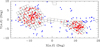 |
Fig. 1. Distribution of the AC data set in Magellanic Clouds. Red points are stars present in the VMC, while blue points are ACs from OGLE or Gaia with no VMC counterpart. The projection is a zenithal equidistant projection. The center is at RA = 55 deg, Dec = −73 deg. The empty black boxes show the footprint of the VMC survey. |
In this study, the AC light curves typically have five to six epochs in Y and J, and 14-15 in Ks, as illustrated in Fig. 2. In some cases, the number of epochs is larger, particularly when a variable star is positioned on the overlapping area of two neighboring VMC tiles, effectively doubling the number of epochs. Table 1 presents an example of a typical time series photometry in the J band. The complete table with Y, J, K time series photometry for ACs can be accessed at the Centre de Données astronomiques de Strasbourg (https://cds.u-strasbg.fr/).
Example of five epochs of the time series photometry for the star OGLE-SMC-ACEP-062 in the J band. The machine-readable version of the full table is available online at CDS.
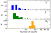 |
Fig. 2. Number of epochs in the VMC Y, J, Ks bands for our AC sample. |
3. Data analysis
To phase the time series photometry for each target, we adopted the period and epoch of peak brightness from the literature (OGLE IV and Gaia DR3, as explained above). Figure 3 illustrates samples of light curves for the F and 1O mode ACs. The approach we used to determine the YJKs intensity-averaged magnitudes follows the methodology described in Ripepi et al. (2016, 2017, 2022) and S24. Specifically, we adhered strictly to the approach detailed in S24, which is briefly summarized in this section.
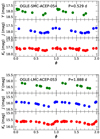 |
Fig. 3. Examples of light curves (used to create templates) for different AC types. From the top: One 1O pulsator and one F pulsator in the Y (green), J (blue), and Ks (red) bands, respectively. We note that the photometric errors are smaller than the dot size, and the light curves have been doubled to shape them better. |
3.1. Template derivation and fitting to the light curves
The intensity-averaged mean magnitudes for pulsating stars were calculated using the template-fitting method. This procedure is crucial because the majority of the sample has a number of epochs ≤10, especially in Y and J bands.
The templates are derived from light curves that have more than ten epochs. As outlined in S24, the fitting of light curves to create the templates is executed in three phases: (i) The well-sampled light curves selected by visual inspection are fit by employing a spline function. (ii) The spline function is rescaled to have a mean magnitude equal to zero and a peak-to-peak amplitude equal to one. iii) A ten-term truncated Fourier series is fit to the spline curve. The coefficients (amplitudes and phases) are provided in Appendix B.
The final template sample, illustrated in Fig. 4, comprises 6, 5, and 11 models for the Y, J, and Ks bands, respectively. These templates were further categorized by pulsation mode (F, 1O) for each band. Fewer templates are present in the Y and J filters compared to the Ks filters because these bands have fewer observational epochs (see Fig. 2).
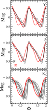 |
Fig. 4. Templates created in every band: Y (top), J (middle), and Ks (bottom). |
As in S24, the procedure for fitting each light curve with a template requires determining three parameters: (1) a magnitude shift, δM; (2) a scaling factor, a, that increases or reduces the template amplitude to match that of the observed light curve; and (3) a phase shift, δϕ, that takes into account possible differences in phase between templates and observed light curves. These three unknowns for each template are retrieved by minimizing the following χ2 function:
![Mathematical equation: $$ \begin{aligned} \chi ^2 = \sum _i^{N_{\rm pts}} \frac{[m_i - (a\times M_t(\phi _i + \delta \phi )+ \delta M)]^2}{\sigma _i^2}. \end{aligned} $$](/articles/aa/full_html/2025/07/aa54854-25/aa54854-25-eq1.gif) (1)
(1)
Here, Npts is the number of epochs; mi, ϕi, and σi are the observed magnitudes, the corresponding phases, and uncertainties on the magnitudes, respectively; and Mt(ϕi) is the template. Outliers are detected by analyzing the distribution of the residuals from the fit and identifying points outside the interval −3.5 × DMAD to +3.5 × DMAD, where “DMAD” is the double-median absolute deviation4.
Similar to our previous studies, we assessed the uncertainties using a Monte Carlo method. The errors in our fit parameters were determined by the robust standard deviation (1.4826 ⋅ MAD) derived from the distributions generated by the bootstrap simulations. The resulting accurate intensity-averaged magnitudes (and amplitudes) in all the bands for the 193 ACs are shown in Table 2, while examples of fit light curves are shown in Fig. 5.
Photometric parameters from the VMC survey for all the 198 LMC and SMC ACs analyzed in this paper.
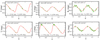 |
Fig. 5. Examples of template-fit AC light curves in the Y, J, and Ks bands (left to right columns). The green-filled circles are the observations, the red solid line is the best template for the light curve, and black-filled circles are the outliers not used in the fit. |
3.2. Reddening estimates for the target stars
We corrected for interstellar extinction using the reddening maps published by Skowron et al. (2021). These maps have a spatial resolution ranging from 27″ × 27″ in the peripheries to 1 7 × 1
7 × 1 7 in the centers of the Magellanic Clouds. Since these maps do not cover the entire extent of the LMC and the SMC, they were complemented by Schlegel et al. (1998, SFD) maps with a lower spatial resolution (6
 1). Table 2 reports not only the value of E(V − I) but also a flag “EVI”, where 0 and 1 respectively indicate the use of SFD or Skowron et al. (2021) maps.
The extinction correction requires an assumption on the reddening law and RV value, and we note that there are different reddening laws discussed in the literature (e.g., Cardelli et al. 1989; Fitzpatrick 1999; Gordon et al. 2003; Wang & Chen 2023). To ensure consistency and comparison with our previous works (Ripepi et al. 2012, 2014, 2015; Ripepi et al. 2016, 2022, S24), we decided to adopt the extinction coefficients from Cardelli et al. (1989) and RV = A(V)/(A(B)−A(V)) = 3.235. For the Gaia bands, we used the coefficients published by Casagrande & VandenBerg (2018) based on Inno et al. (2013). The impact of different reddening laws on the PWJK relations is discussed in the Appendix C. The resulting coefficients to be multiplied by E(V − I) to obtain the dereddened magnitudes in different bands are the following:
-
In the GBP band, 2.678;
-
In the V band, 2.563;
-
In the G band, 2.175;
-
In the GBP band, 1.615;
-
In the I band, 1.564;
-
In the Y band, 1.00;
-
In the J band, 0.744;
-
In the Ksband, 0.308.
3.3. Complementary optical data
The VMC NIR data were complemented by optical photometry from the literature. This allowed us to examine changes in the PL relationships across different wavelengths and to build Wesenheit magnitudes by combining optical and infrared bands. Specifically, V and I bands were obtained from the OGLE IV survey, whereas the G, GBP, and GRP bands were provided by Gaia DR3 (Ripepi et al. 2023). All optical data are presented in Table 3.
Optical photometric parameters for all 198 LMC and SMC ACs analyzed in this paper.
As in Table 2, the flag “SOURCE” in Table 3 indicates whether the object was identified by OGLE IV or Gaia. The flag “SOS” concerns the derivation of the average magnitudes in the Gaia bands6: the value 0 indicates that the standard technique was adopted (see, e.g., Evans et al. 2018) without any specific assumption for pulsating variables; the value 1 means that the averaged-intensity technique through modeling the light curves was adopted (e.g., Clementini et al. 2016). The 193 ACs with OGLE IV identification have at least one magnitude collected by Gaia: 42 and 152 with a flag “SOS” value of 0 and 1, respectively. The flag “VI” in Table 3 indicates the origin of the V I magnitudes. In the OGLE IV catalog, all the stars have the average I band magnitudes, while all do not have the V measurement. Moreover, the V, I data is completely missing for the six stars originating from the Gaia catalog and not present in OGLE IV. The missing values for the V, I bands were recovered through the photometric transformations between Johnson and Gaia filters provided by Pancino et al. (2022, hereinafter P22). The stars with photometry from the OGLE IV survey have the flag “VI” equal to OGLE,OGLE. When the V is estimated from Gaia due to missing OGLE data, the “VI” flag is “P22;OGLE.” For the stars identified only by Gaia, the “VI” flag is equal to “P22;P22.” The V I magnitudes estimated from the Gaia bands have a lower quality if the flag “SOS” is 0.
4. Period-luminosity and period-Wesenheit relations
The multiband photometry allowed us to calculate PL and PW relations for the ACs separately for the LMC and SMC. The list of PW relations considered in this study is thefollowing:
-
PWVI = V − 2.54 (V − I) ;
-
PWVKs = V − 1.13 (V − Ks) ;
-
PWJKs = Ks − 0.69 (J − Ks);
-
PWYKs = Ks − 0.42 (Y − Ks);
-
PWG = G − 1.90 (GBP − GRP).
The coefficient of the PW relation was calculated as Rλ1/Rλ1 − Rλ2. This excludes the coefficients of the PW in the Gaia bands, which is 1.90 according to Ripepi et al. (2019).
4.1. PL and PW relations derivation
The observed quantities, namely the dereddened intensity averaged magnitudes and the periods, were fitted with the following linear relations to determine the coefficients of the PL and PW relations:
 (2)
(2)
To carry out these linear fits in one dimension, we adopted the Python code for least trimmed squares (LTS; Cappellari et al. 2013). This method makes the fit converge to the correct solution even in the presence of numerous outliers, which can cause the much simpler σ-clipping approach to converge to the wrong solution.
4.2. Results for the PL and PW relations
Figure 6 shows the observational data used for deriving the PL relations for the LMC in the NIR bands. Likewise, all the data available for computing the PL and the PW relations in the LMC and SMC are available in Fig. E1 in the Appendix E. Throughout these figures, the two types of pulsators are distinguished using different colors.
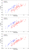 |
Fig. 6. Period-luminosity relations in the NIR bands for the ACs in the LMC. Red and blue filled circles represent F and 1O mode ACs, respectively. We note that the error bars are smaller than the size of the dots. |
A visual examination of the figures revealed several distinct features that we later quantitatively validated. For the LMC PL relations, the dispersion of the data decreases from the optical to NIR bands. As expected, this trend is not observed in the SMC PL relations because the dispersion is dominated by the large depth of the galaxy along the line of sight (e.g., Subramanian & Subramaniam 2015; Ripepi et al. 2017). The PW relations in nearly all cases are tighter than those of the PLs (see, e.g., De Somma et al. 2022), except for the PL relations in the J and Ks bands, which in the LMC have a dispersion comparable to that of the PW relations. In the LMC and in the SMC, the slopes followed by the F and the 1O pulsators appear the same, while the respective zero points differ, as expected.
We derived the coefficients of the PL and PW relations for F and 1O ACs. We first did so separately to quantify the differences in the slopes between the different modes of pulsation and then together (see Sect. 4.3) to assess the possibility of combining the two subsamples. Figure 7 displays select tight PL and PW relations for the F mode AC in the LMC. The fit results for all the considered PL and PW relations are reported in Table 4, while the figures showing the fit PL and PW relations are in Appendix E (Figs. E2 and E3) for the LMC and the SMC, respectively. In the subsequent analyses, we used the relations that present the smallest dispersion: PL relations in the J and Ks bands and the PW relations in Ks, J − Ks, and G, GBP − GRP. These are highlighted in Table 4.
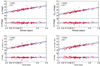 |
Fig. 7. Example best fits for the F ACs in the LMC. From left to right, we show in the top panels the PLJ and the PLKs relations, and in the bottom panels, we show the PWJKs and the PWG relations, respectively. The red and gray filled circles are the data used for the fit and the outliers. The solid black line is the best fit to the data, while the dashed blue lines show the ±1σ levels. Upper panels and lower panels in each figure contain the fits and the residuals of the fit, respectively. The fits for the other bands are in the Appendix E. |
Coefficients of the PL and PW relations for ACs in the LMC and the SMC.
4.3. Fundamentalization of first overtone Anomalous Cepheids
In the previous section, we calculated the PL and PW relations for F and 1O ACs separately. However, it is sometimes convenient to determine such relations for both modes of pulsation together, especially when the number of objects is not large. The so-called fundamentalization of the 1O periods has been carried out in the literature extensively for CCs (e.g., Feast & Catchpole 1997) and RRL (e.g., Marconi et al. 2015) variables but thus far not for ACs.
To fundamentalize the 1O mode AC pulsators in the LMC, considering that they cover a similar period to the RRL pulsators and belong to the same central helium-burning evolutionary phase (having ignited helium in degenerate conditions), we first tried to use the standard value from the literature for 1O RRL stars (RRc type), namely log(1/R) = 0.127 (see, e.g., Marconi et al. 2015, and references therein). However, the resulting distribution in the PL and PW planes seems to suggest that a higher correction should be applied to 1O mode ACs with respect to the RRc pulsators. This difference should be ascribed to the different envelope structures of ACs, which are relatively more massive and expanded than RR Lyrae stars, thus modifying the relation between the mean density and the periodicities of the first two radial modes, as well as their difference. Indeed the value of R that minimizes the dispersion of the PL and PW relations for the combined F+1O mode AC sample in the LMC is log(1/R) = 0.145. Since the fundamentalization of the 1O mode pulsators in the PL and PW relations is independent of temperatures and luminosities (see, e.g., Pilecki 2024), the R value is first obtained using the PL relations in the NIR bands, which are the tightest ones, and then verified in all other PL and PW relations. In the following analysis, we use this revised value of log (1/R) to generate a collective sample of F+10 mode AC pulsators.
Figure 8 displays examples of select PL and PW relation fits for the combined F+1O sample after fundamentalization of the 1O mode periods, while the results of the best fitting procedure are listed in Table 4. The figure shows that also for the combined sample, the tightest relations are the PL relations in the NIR and PW relations in all the bands.
 |
Fig. 8. Example of fits for the F and 1O ACs in the LMC after 1O ACs were fundametalized by adding 0.145 to the logarithm of their periods. Each row contains two figures displayed in the left and right panels, respectively, in the following order: PLY, PLJ, PLKs, PWVI, PWVKs, PWG, PWYK, and PWJKs. For each figure, the upper subpanel shows the best-fitting line, while the lower subpanel reports the fit residuals. Red and blue filled circles represent the F and 1O mode ACs, respectively. The gray filled circles are outlier objects not included in the fit. The solid black line is the best fit to the data, while the dashed blue lines show the ±1σ levels. The best fits in additional bands can be found in Appendix E. |
5. Results
In this section, we analyze the PL and PW relationships calculated in this work. First, we explore how the PL and PW coefficients vary with wavelength. Subsequently, we compare our findings with the predictions of pulsation theory and empirical literature studies. Finally, after calibrating our most accurate relationships using an assumed LMC distance, we calculate thedistances to specific MW globular clusters and nearby galaxies containing AC variables. An additional calibration of the AC PW relations based on select Galactic field AC stars with reliable multiband photometric data and Gaia parallaxes is discussed at the end of this section.
5.1. Wavelength dependence of the PL coefficients
The extensive set of PL and PW relations shown in Table 4 allowed us to investigate how the slopes and dispersion of these relations vary with wavelength and to choose the best relationships to use in further analysis. The slopes and dispersion of the PL relations increase (in absolute value) and decrease, respectively, as the wavelength increases. While this trend is already known in the literature for the CCs (Madore & Freedman 1991) and T2Cs (S24), this work provides the first clear confirmation for the ACs. The physics behind this anticorrelation was noted for the CCs by Madore & Freedman (1991) and was explained physically by Madore & Freedman (2012). This feature is due to the different surface brightness dependences on the effective temperature at different wavelengths.
Figure 9 shows the result of this investigation for the PL relations for the separate LMC F and 1O mode ACs and the combined F+1O ACs (using fundamentalized periods for the 1O). Looking at the panels displaying the α (relative zero point), β (slope), and σ (dispersion) coefficients in each figure, the above-mentioned trends stand out clearly, especially for theF+1O case.
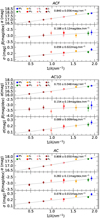 |
Fig. 9. From top to bottom: Dependency of the LMC PL relation zero point, slope, and dispersion, respectively, as a function of 1/wavelength. |
The dependences of the slope and dispersion on the wavelength are slightly less evident in Fig. 10 for the SMC. Indeed, the significant depth along the line of sight (∼0.17 mag, e.g., Ripepi et al. 2017) produces an additional dispersion due to the geometry of the system that can be larger than the intrinsic width of the IS. The influence of the SMC depth is more evident in the case of the F mode ACs (Fig.10).
5.2. Absolute calibration of the PL and PW relations using the geometric distance to the LMC
Calibrating the PL and PW zero points (intercepts) in absolute terms is mandatory to compare them with literature values as well as to calculate distances. To carry out this crucial procedure, we decided first to use the geometric distance modulus of the LMC (μLMC = 18.477 ± 0.026 mag) as measured by P19 based on a sample of eclipsing binaries.
The calibrated PL and PW relations are listed in Table 5, while Table C1 in Appendix C shows the coefficients of the PWJK in the LMC starting from different extinction laws. Whereas the relative zero points based on three different extinction laws (Wang & Chen 2023; Cardelli et al. 1989; Fitzpatrick 1999) agree within 2σ, the impact on the absolute zero points, where the uncertainty of the geometric distance modulus of the LMC is also taken into account, is less than 1σ.
Comparison between present results for ACs in the LMC, the SMC, and the literature.
5.3. Comparison with the literature
At this point, the relations with absolute intercepts as presented in the previous section and the ones listed in Table 4 (with relative intercepts) can be compared to those available in the literature for the LMC and the theory. Table 5 shows a comparison of the values derived in this paper and a variety of PL and PW relation values from the literature (R14, Marconi et al. 2004; Groenewegen & Jurkovic 2017; Iwanek et al. 2018). Marconi et al. (2004) presented theoretical PL relations for ACs in optical bands based on nonlinear convective pulsation models. R14 exploited a subset of VMC data in 11 tiles in the LMC and derived PL and PW relations in the V, I, and Ks bands. Groenewegen & Jurkovic (2017), using the data collected in the OGLE III survey, published PL and PW relations for the ACs in the LMC, while Iwanek et al. (2018) used the complete OGLE AC sample in the LMC and the SMC.
A review of the table allowed us to affirm that the slopes and the intercepts derived in this work for the PL and PW relations are in agreement with the literature studies within 1-2σ of the reported errors. The greatest difference for the PL coefficients was observed in the V band; for the slopes of the PL, it was in the Ks band; and for the PW, it was in the VKs combination with R14. Our PL and PW relations were derived from the largest sample of stars for each pulsation mode and filter combination. In particular, our AC sample is more than twice the size of the R14 sample.
The comparison with the literature shown in the table is encouraging. The agreement between different studies based both on theory and observation demonstrates that the ACs are reliable and precise distance indicators when compared within the same stellar systems. In Section 6, we apply PL and PW relations to the MW GGCs and LG galaxies, where additional factors such as metallicity may come into play.
5.4. The LMC distance modulus through absolute calibration of the PW relations using Gaia parallaxes
An independent calibration of selected PW relations for ACs can be derived using Gaia parallaxes for a sample of Galactic ACs. In this way, we can use the ACs to obtain the distance modulus to the LMC instead of assuming it. To carry out this exercise, we decided to use two of the best PW relations, namely those based on the Gaia and the J, Ks bands. The procedure is composed of several steps. The first step was to determine average magnitudes in the J, Ks bands for Galactic ACs (for detailed description of the method, see Appendix D). The second step involves calibration of the PW relations based on the average magnitudes.
To calibrate the Galactic AC PW relations, we could not simply invert the Gaia parallaxes (e.g., Luri et al. 2018). Instead, as in S24, we adopted the photometric parallax (Feast & Catchpole 1997) to carry out the calculations. The photometric parallax (in mas) is defined as
 (3)
(3)
where m is the apparent magnitude (the apparent Wesenheit magnitude in our case), and M is the absolute magnitude (or absolute Wesenheit magnitude) defined as
 (4)
(4)
Here, β is the slope that we obtained in two ways. In the first case, we fixed β to the values obtained for the LMC (listed in Table 47). The value of α was obtained by minimizing the following χ2 expression:
 (5)
(5)
where ϖEDR3 are the parallaxes from Gaia EDR3 corrected individually with the recipe provided by Lindegren et al. (2021). A comprehensive description of the fitting process can be found in Ripepi et al. (2022), and it is not reiterated here.
Distances to the LMC for the fixed slope of the PW relations for MW ACs.
We calculated the PW relations, adopting three values of the counter zero-point offset to be applied to the Gaia parallaxes: ϖZP = 0 mas, −0.014 mas, and −0.022 mas, i.e. no counter offset and progressively larger values, according to Riess et al. (2021) and Molinaro et al. (2023), respectively. The resulting values for the intercept α are listed in Table 6.
In the second case, we left both α and β free to vary while minimizing Eq. (6). Again, we repeated the calculation for the three values of the parallax counter-correction discussed above. The results for α and β and their errors are shown in Table 7. The σ term at the denominator of Eq. (6) is the sum in quadrature of the uncertainties on both ϖEDR3 and ϖphot.
Distances to the LMC without fixing the slope of the PW relations for the MW ACs.
A comparison between Tables 6 and 7 revealed that not fixing the slope of the PW relations leads to large errors on the β values. The large uncertainties prevented us from drawing any firm conclusion from this occurrence. The differences in the values of α are less important, and they agree within 1σ.
In Tables 6 and 7, we have several PW relations. To verify which is the most accurate, we again used the geometric distance modulus of the LMC by P19 as a reference. From the periods of the LMC ACs in our sample, we calculated the absolute Wesenheit magnitudes for each star. In the formula μ = m − M, we applied these absolute Wesenheit values and the corresponding apparent magnitudes calculated in this paper, and we calculated the individual distance moduli of the ACs in the LMC. Figure 11 shows the distributions of the inferred distance moduli for the LMC ACs. The different colors refer to the different parallax counter zero-point offsets applied to Gaia DR3 parallaxes before minimizing Eq. (6).
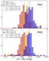 |
Fig. 11. Distribution of the inferred LMC absolute distance moduli calibrated through Gaia DR3 MW AC parallaxes. The red histogram corresponds to the values obtained using MW AC parallaxes with no counter zero-point offset, while the red vertical line is the median of the distribution. The orange and blue histograms and vertical lines are the same as the red ones but were respectively derived using the counter zero-point offsets ϖZP = −0.014 mas, as suggested by Riess et al. (2021), and ϖZP = −0.022 mas, as suggested by Molinaro et al. (2023). |
The average LMC distance moduli (μLMC) and the relative errors (RMS of the mean) are listed both in Table 6 and Table 7, respectively, for the three parallax counter-offset values. The MW AC parallaxes seem to need a counter zero-point offset as large as ϖZP = −0.022 mas to obtain an average LMC distance modulus in agreement within 1σ with the LMC geometric value of 18.477 ± 0.026 mag (P19) and the canonical distance modulus of 18.49 ± 0.09 mag suggested by de Grijs et al. (2014). However, the PW relations at the basis of our LMC distance modulus do not take into consideration possible metallicity dependence. This additional term may play a role in the absolute calibration of the PW relation through the MW AC Gaia parallaxes.
5.5. The LMC-SMC relative distance modulus
Given the agreement among almost all the slopes for the LMC and the SMC (see Table 4), it is possible to calculate the relative distance of the two Magellanic Clouds. Figure 12 illustrates the adopted technique for the case of the PL in the Ks band. In practice, we compared the PL relations for the LMC and the SMC, calculating the Δμ as the difference of the zero points, for the F mode (top panel), the 1O mode (middle panel), and the F mode plus the fundamentalized 1O mode (bottom panel) ACs. Similar figures for the comparison through PWJKs and PWG relations can be found in the Appendix E.
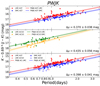 |
Fig. 12. Comparison between the LMC and SMC PWJK relation to determine the relative distances (see labels). In the top panel, red and blue filled circles are, respectively, the LMC and SMC F mode ACs, while the red and the blue solid lines are the fitted PL relations in the corresponding Cloud. In the middle panel, the green and yellow filled circles are respectively the LMC and SMC F mode ACs, while the green and the yellow solid lines are the fitted PL relations in the corresponding Cloud. In the bottom panel, the red filled and empty circles are respectively the LMC F mode and fundamentalized 1O mode ACs; blue filled and empty circles are respectively the SMC F mode and fundamentalized 1O mode ACs, while the red and the blue solid lines are the fitted PWJK relations in the corresponding Cloud. |
Table 8 reports the relative distance between the LMC and the SMC, and the SMC absolute distance obtained by adding the geometric LMC distance (P19) to the Δμ. Our absolute SMC distances are in agreement within 2σ with the SMC geometric distance (18.977 ± 0.032 mag) provided by Graczyk et al. (2020) and the mean value of 18.96 ± 0.02 mag from de Grijs & Bono (2015). The difference between our SMC distance modulus and that of the literature might be attributed to a metallicity dependence, which is not included in our study due to a lack of spectroscopic data for ACs. Although we know that ACs in the Milky Way are metal poor (Ripepi et al. 2024), in the LMC and SMC, their metallicity is not known. These galaxies present a significant metallicity spread (Povick et al. 2023), and therefore spectroscopy is needed to establish appropriate [Fe/H] values for their ACs. Furthermore, as suggested by Breuval et al. (2024), a metallicity term needs to be added to the CC PW relations to retrieve the SMC distance modulus in agreement with the geometric distance modulus (Graczyk et al. 2020).
Relative distances between the LMC and SMC, and the absolute SMC distance modulus calibrated through the LMC geometric distance modulus by P19.
6. Application of PL and PW in the Milky Way and Local Group
To test the PW relations derived in this work, we applied them to GGCs and dSph galaxies hosting ACs. Accurate GGC distances can be derived from a variety of methods (see, e.g., Baumgardt & Vasiliev 2021, and references therein). On the other hand, although the dSphs in the LG are rich in ACs, NIR photometry is available only for the Draco dSph (see below), which limits the possibility of testing the PW relations.
6.1. Anomalous Cepheids in Galactic globular clusters
Up to now, only two ACs have been confirmed as members in a GGC, namely V7 in M92 and V19 in NGC 5466 (see, e.g., Ngeow et al. 2022). For M92 V7, we adopted the accurate NIR photometry by Del Principe et al. (2005), while for NGC 5466 V19, we only have 2MASS single-epoch photometry.
Two additional variable stars, V68 and V84, in omega Centauri (ωCen) have been indicated as candidate ACs in the literature (see, e.g., Navarrete et al. 2015, and reference therein). To verify whether these two stars could be ACs that belong to ω Cen, we first checked if their proper motions from Gaia are consistent with the proper motions of the bulk of ω Cen members. This allowed us to immediately reject V84 as a field star, and we kept V68 for further analysis. To that aim, we adopted the accurate NIR photometry by Braga et al. (2016). Using Gaia DR3 data, Cruz Reyes et al. (2025) recently identified seven new candidate ACs in GGCs (not including the two stars in ω Cen discussed above). These cluster members, previously known as T2Cs, were reclassified as ACs based on their positions close to or on the PW relation in the Gaia bands. We searched the literature for NIR photometry of these objects. We were not able to find it for NGC 2419 V19 or NGC 6388 V29. The 2MASS data are not useful because the former cluster is very distant with respect to other GGC distances, whereas NGC 6388 has extremely crowded central regions. For the remaining five stars, the source of the NIR photometry is reported in Table 9 along with data for the three ACs in M92, NGC 5466, and ω Cen.
Candidate ACs in GGCs. “Flag NIR” indicates the source of the NIR photometry, and “ID” lists the Gaia DR3 identification according to Gavras et al. (2023).
For M92 V7, Terzan 1 V4, and ω Cen V68, we found in the literature average NIR magnitudes from multi-epoch data, as specified in Table 9. For the remaining five stars, we have only single-epoch photometry from either the 2MASS or VHS DR5 (VISTA Hemisphere Survey Data Release 5; McMahon et al. 2013) surveys. For these objects we computed the intensity-averaged magnitudes using the template technique as described in Appendix D. However, the period and epoch of maximum light are available only for NGC 6752 V1 based on ASAS-SN data (All-Sky Automated Survey for Supernovae Shappee et al. 2014; Christy et al. 2023) and for M22 V11 in the Gaia catalog (see Ripepi et al. 2023). The J and Ks magnitudes of these two objects in Table 9 are intensity-averaged magnitudes obtained from the template-fitting technique. For NGC 6388 V18 and NGC 2808 V29, we adopted the single-epoch J and Ks magnitudes from VHS DR5 and included a conservative error of 0.15 mag to account for the random phase.
This NIR photometry allowed us to use our best PL and PW relations (namely the PWJKs, PLJ, and PLKS) calibrated with the geometric distance of the LMC to verify the AC nature of these GGC stars. Figure 13 shows the results. The confirmed and candidate ACs in the GGCs are plotted with different colors and compared with the PL and PW relations for the F and 1O mode ACs derived in this work and for the T2Cs as published by S24. In all the cases, these relations have the zero point anchored to the geometric distance modulus of the LMC by P19. To calculate the absolute magnitudes for the GGC ACs, we adopted the distances by Baumgardt & Vasiliev (2021) and the reddening values by Harris (2010), reported in Table 9.
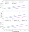 |
Fig. 13. Position of the known and candidate ACs in GGCs from Cruz Reyes et al. (2025) in the PL and PW relations for ACs and T2Cs in the LMC. In the top panel, the green and blue lines are for the 1O mode and F mode ACs, and the magenta lines are for the T2Cs PLJ relations in the LMC, calibrated with the LMC distance modulus by Pietrzyński et al. (2019), respectively. Blue, orange, green, violet, brown, gray, light green, and cyan-filled circles are the known and candidate ACs in ωcen, Terzan1, NGC6752, NGC6388, NGC5466, NGC2808, M92, and M22. The middle and bottom panels show the same as for the top panel but for the PLKs and PWJKs relations, respectively. The NIR photometry for M92 is from Del Principe et al. (2005). |
Draco distance moduli based on our PL and PW relations and Bhardwaj et al. (2024) NIR photometry.
A inspection of this figure led to the following observations and conclusions. The known ACs in GGCs, namely M92 V7 and NGC 5466 V19, lie on top of the LMC PL and PW relations for F and 1O mode ACs, respectively. This means that their AC nature is confirmed and that the distances of the two clusters agree within 1σ with the distance scale of ACs devised in this work (in the figure the shaded regions report the 1σ uncertainty of the PL and PW relations).
The candidate AC M22 V11 lies on all the F mode AC PL and PW relations of Fig. 13 and can therefore be considered the third confirmed AC in a GGC. Also, the distance of M22 appears to be in agreement with the LMC distance scale.
Our data provide non-conclusive results for NGC 6752 V1. Compared with the PLJ, the V1 J magnitude is in agreement with the T2C relationship. Compared with the PLKs, the V1 Ks magnitude is placed between the T2C and AC F mode relationships, while in the PWJ Ks, it lies on the AC F mode locus. In conclusion, we cannot prove or disprove the AC nature of this star.
The star Terzan 1 V4 is not an AC but a T2C, as previously reported in the literature. On the other hand, the extremely high reddening in the direction of this cluster makes it difficult to estimate the dereddened magnitude in the optical (Gaia) bands. Indeed, in this regime, even the Wesenheit magnitude could include significant uncertainty due to the possible non-standard value of the total-to-selected extinction ratio RV.
NGC 6388 V18 and NGC 2808 V29 are located at a significantly higher luminosity compared to all the AC PL and PW relations of Fig. 13. This could be explained by each of the two variable stars being significantly blended with a red source. Such blending would not be surprising because the two clusters are severely crowded in their central regions, and the main contaminants are red giant stars. Nevertheless, this prevents us from drawing any firm conclusion regarding the nature of these stars.
ω Cen V68 has a period that makes it unlikely to be an F mode AC, but it is too faint to be a 1O mode AC. It is therefore likely that this star is an evolved RRL.
6.2. The distance to Draco
The Draco dSph hosts nine ACs, as suggested by Muraveva et al. (2020). However, only five have been observed in the NIR. Bhardwaj et al. (2024, hereinafter B24) published accurate NIR photometry for four F and one 1O mode ACs as well as for 336 RRL stars in Draco. This allowed us to make an independent comparison of the RRL star and AC distance scales.
We first fundamentalized the unique AC 1O mode pulsator to obtain a total sample of five pulsators, which we then used to derive the distance modulus of Draco. Table 10 lists our final estimates of the Draco distance modulus, while Figure 14 compares our best value based on the PWJK relation with those from the literature. Our estimate for the Draco distance modulus is in agreement within 2σ with all the recent and past distance estimates8 and within 1σ with Nagarajan et al. (2022), Muraveva et al. (2020), Hernitschek et al. (2019) and B24. In more detail, by assuming our new AC PL relations instead of the R14 ones, the difference between the RRL-based and the AC-based distance moduli of Draco reduced from 0.17 mag, according to B24, to 0.13 mag. Notably, B24 suggested that by assuming a metallicity difference of Δ[Fe/H] = 0.5 dex between the LMC and Draco AC abundances, the entire distance discrepancy could be explained with a metallicity dependence of the PL and PW relations of ∼−0.34 mag/dex, a value typical for CCs (see, e.g., Riess et al. 2024; Trentin et al. 2024). This value would slightly decrease to ∼−0.26 mag/dex in our case. However, current pulsation models (e.g., Marconi et al. 2004) do not predict a significant metallicity dependence of the AC PL relations, and the AC PL and PW relations presented in this work and those by R14, as already discussed above, do not include this parameter.
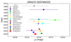 |
Fig. 14. Comparison of different Draco distance moduli. The reference values are taken from Stetson (1979), Nemec (1985), Aparicio et al. (2001), Bellazzini et al. (2002), Bonanos et al. (2004), Cioni & Habing (2005), Kinemuchi et al. (2008), Sesar et al. (2017), Hernitschek et al. (2019), Muraveva et al. (2020), Nagarajan et al. (2022), Bhardwaj et al. (2024). A red star shows the distance modulus to Draco obtained in the present work. |
The hypothesis of a significantly different average metallicity between Draco and the LMC is, however, plausible, considering that different metallicities can be linked to very different star formation histories of these two galaxies (e.g., Aparicio et al. 2001; Mazzi et al. 2021, for Draco and LMC, respectively). Furthermore, we showed that LMC and SMC distance moduli based on AC PW relations need an a posteriori correction to align them with the corresponding geometric distance moduli.
In addition, according to the bottom panel of Figure 12, the LMC-SMC relative distance modulus needs an increase of 0.10 ± 0.04 mag to recover the LMC-SMC relative distance modulus as derived by using eclipsing binaries. The metallicity difference is larger between the LMC (Choudhury et al. 2021) and Draco (Choudhury et al. 2020) than between the LMC and the SMC (Choudhury et al. 2020) and supports the evidence of a larger scatter in the comparison of the Draco distances. These evidences call for further empirical tests based on spectroscopic data to verify the dependence of the AC PL and PW relations on metallicity.
7. Summary and conclusions
In this study, we have presented and exploited the Y, J, and Ks time series photometry from the ESO public survey VMC for a sample of approximately 200 ACs located in the LMC and SMC. The VMC data were complemented with optical data from the OGLE IV survey and the Gaia mission. From these surveys, we obtained the identifications and positions of the pulsators, their periods, their modes, and their photometry (and amplitudes where possible) in the V, I, G, GBP, and GRP bands.
After selecting the stars with the best-quality VMC time series, we constructed a set of light-curve templates for F mode and 1O mode ACs. These templates were employed to derive accurate intensity-averaged magnitudes (and amplitudes, when possible) for all the pulsators at our disposal through a rigorous pipeline previously developed in the context of VMC studies of CCs and T2Cs.
The final Y, J, and Ks photometry, along with the aforementioned optical data, were used to create a large set of PL and PW relations for both F and 1O mode ACs. The same relations were also calculated for the global F+1O mode sample. This was achieved by fundamentalizing the 1O mode period with a value of P1O/PF = 0.716. This ratio has been found in this work for the first time for ACs. The possibility of using the total sample of ACs increases the statistics of the PL and PW relations in all stellar systems hosting both F and 1O mode ACs.
We investigated the dependences of the PL relations – namely the slopes and the dispersions – on the adopted wavelength for the first time. Similar to the case for CCs and T2Cs, our findings demonstrate that also for the ACs, the slope increases and the dispersion decreases as one moves toward longer wavelengths.
In general, our PL and PW relations are in agreement with the predictions of the pulsation theory, while the coefficients of the PL and PW relations are consistent within better than 2σ for both the LMC and the SMC compared to the literature. The evidence suggests that ACs are precise and reliable distance indicators.
We calibrated the PL and PW relations using a sample of Galactic field ACs for which 2MASS single-epoch observations were available. Thanks to our set of light-curve templates, the single-epoch magnitudes were transformed into mean magnitudes. To calculate the absolute distance to the LMC, we followed two procedures: fixing the slopes to those of the LMC and not fixing the slopes. In both cases, we calculated the zero points of the PL and PW relations using the Gaia EDR3 parallaxes. As a result, we obtained a μLMC that is within 1σ of the geometric estimate provided by P19, particularly when adopting a counter zero-point offset for the Gaia parallaxes of about −22 μas. Alternatively, an additional metallicity term in the PL and PW relations might compensate for such a counter zero-point offset.
The tightest relations derived in this work, namely the PL in the Ks band and the PW relations in the J, Ks, and Gaia bands in the LMC and the SMC, served to calculate the relative distance between the Magellanic Clouds, which we find to be within 2σ of the literature values. Our relative tightest relations for the LMC ACs were calibrated using the LMC geometric distance modulus. These absolute relations were used to study the ACs in GGCs and in Draco dSph. First, we examined new candidate ACs in GGCs, confirming that M22 V11 is an F mode AC. No firm conclusion could be reached for NGC 6752 V1, NGC 6388 V29, and NGC 2808 V29. The photometry of the last two objects is likely highly contaminated by close luminous red sources. Terzan 1 V4 and ω Cen are respectively a T2C and an RRL. Concerning the known ACs in GGCs M92 V7 and NGC 5466 V19, we confirmed their AC F and 1O mode nature. Their location on the PL and PW relations calibrated on the LMC allowed us to verify that the distance scale of GGCs by Baumgardt & Vasiliev (2021) agrees within 1σ with our ACs based distances.
The application of our NIR PL and PW relations to the five ACs in the Draco dSph (the only dSph for which NIR photometry is currently available) allowed us to determine its distance modulus, which is μDraco = 19.425 ± 0.048 mag (from PWJ Ks) and in agreement with B24. We confirm that the distance modulus to Draco calculated from RRLs is about 0.1 mag larger than that obtained from ACs. In agreement with B24, we suggest that this may be due to a metallicity difference between Draco and LMC ACs.
Proprietary Ultraviolet and Visual Echelle Spectrograph data (P.I. V. Ripepi) for several dozen Galactic ACs, together with upcoming large spectroscopic surveys such as 4-metre Multi-Object Spectroscopic Telescope and Wide-field Spectroscopic Telescope, will significantly enhance our understanding of these variables. Combined with the improved parallaxes expected from Gaia DR4, these resources will provide the necessary information to refine the AC distance scale and assess the possible impact of metallicity on their PL and PW relations.
Data availability
Full Tables 1, 2, 3, B.1, B.2, and B.3 are available at the CDS via anonymous ftp to cdsarc.cds.unistra.fr (130.79.128.5) or via https://cdsarc.cds.unistra.fr/viz-bin/cat/J/A+A/699/A370
The HB turnover refers to an increase in the effective temperature after its minimum value has occurred for brighter luminosities.
The Wesenheit magnitudes are constructed to be reddening-free by definition (Madore 1982).
A tile in the context of VMC refers to a 1.5 sq.deg region of the sky observed with the VISTA telescope.
The DMAD is calculated by treating the values smaller and larger than the median of the considered distribution separately.
According to Breuval et al. (2024, in their Section 4.1), a change in RV would affect the results by only ∼0.002 mag.
“SOS” stands for specific object studies (see, e.g., Ripepi et al. 2023).
The relations used refer to the LMC ACs with the fundamentalized 1O mode periods, i.e. those with “Mode = All”.
An extensive explanation about all the methods can be found in Bhardwaj et al. (2024).
AAA is the 2MASS quality flag indicating good photometry in the HJK bands.
Acknowledgments
The authors thank the anonymous referee for their comments, which helped improve the quality of the manuscript. We thank Mauricio Cruz Reyes for kindly sharing the results of his paper in submission. We acknowledge useful comments and discussions with Matteo Monelli, Giuliana Fiorentino, and Santi Cassisi. Based on data products created from observations collected at the European Organisation for Astronomical Research in the Southern Hemisphere under ESO program 179.B-2003. This research has used the SIMBAD database operated at CDS, Strasbourg, France ad data from the European Space Agency (ESA) mission Gaia, processed by the Gaia Data Processing and Analysis Consortium. Funding for the DPAC has been provided by national institutions, in particular, the institutions participating in the Gaia Multilateral Agreement. We acknowledge funding from: INAF GO-GTO grant 2023 “C-MetaLL – Cepheid metallicity in the Leavitt law” (P.I. V. Ripepi); PRIN MUR 2022 project (code 2022ARWP9C) ’Early Formation and Evolution of Bulge and Halo (EFEBHO),’ PI: Marconi, M., funded by the European Union – Next Generation EU; Large Grant INAF 2023 MOVIE (P.I. M. Marconi). This research was supported by the Munich Institute for Astro-Particle and BioPhysics (MIAPbP), funded by the Deutsche Forschungsgemeinschaft under Germany’s Excellence Strategy – EXC-2094 – 390783311, by the International Space Science Institute (ISSI) in Bern/Beijing through ISSI/ISSI-BJ International Team project ID #24-603 – “EXPANDING Universe” (EXploiting Precision AstroNomical Distance INdicators in the Gaia Universe), and by INAF-ASTROFIT fellowship. T.S. and G.D.S. thank the Istituto Nazionale di Fisica Nucleare (INFN), Naples section, for support through specific initiatives QGSKY. Finally, this paper is based on work supported by COST Action CA21136, “Addressing Observational Tensions in Cosmology with Systematics and Fundamental Physics (CosmoVerse)”, funded by COST (European Cooperation in Science and Technology).
References
- Aparicio, A., Carrera, R., & Martínez-Delgado, D. 2001, AJ, 122, 2524 [NASA ADS] [CrossRef] [Google Scholar]
- Baumgardt, H., & Vasiliev, E. 2021, MNRAS, 505, 5957 [NASA ADS] [CrossRef] [Google Scholar]
- Bellazzini, M., Ferraro, F. R., Origlia, L., et al. 2002, AJ, 124, 3222 [NASA ADS] [CrossRef] [Google Scholar]
- Bhardwaj, A., Rejkuba, M., Ngeow, C.-C., et al. 2024, AJ, 167, 247 [Google Scholar]
- Bonanos, A. Z., Stanek, K. Z., Szentgyorgyi, A. H., Sasselov, D. D., & Bakos, G. Á. 2004, AJ, 127, 861 [Google Scholar]
- Bono, G., Caputo, F., Santolamazza, P., Cassisi, S., & Piersimoni, A. 1997, AJ, 113, 2209 [NASA ADS] [CrossRef] [Google Scholar]
- Braga, V. F., Stetson, P. B., Bono, G., et al. 2016, AJ, 152, 170 [Google Scholar]
- Breuval, L., Riess, A. G., Casertano, S., et al. 2024, ApJ, 912, L1 [Google Scholar]
- Cappellari, M., Scott, N., Alatalo, K., et al. 2013, MNRAS, 432, 1709 [Google Scholar]
- Caputo, F., Castellani, V., Degl’Innocenti, S., Fiorentino, G., & Marconi, M. 2004, A&A, 424, 927 [NASA ADS] [CrossRef] [EDP Sciences] [Google Scholar]
- Cardelli, J. A., Clayton, G. C., & Mathis, J. S. 1989, ApJ, 345, 245 [Google Scholar]
- Casagrande, L., & VandenBerg, D. A. 2018, MNRAS, 479, L102 [NASA ADS] [CrossRef] [Google Scholar]
- Cassisi, S., & Salaris, M. 2013, Old Stellar Populations: How to Study the Fossil Record of Galaxy Formation (Wiley-VCH) [Google Scholar]
- Choudhury, S., de Grijs, R., Rubele, S., et al. 2020, MNRAS, 497, 3746 [NASA ADS] [CrossRef] [Google Scholar]
- Choudhury, S., de Grijs, R., Bekki, K., et al. 2021, MNRAS, 507, 4752 [CrossRef] [Google Scholar]
- Christy, C. T., Jayasinghe, T., Stanek, K. Z., et al. 2023, MNRAS, 519, 5271 [Google Scholar]
- Cioni, M. R. L., & Habing, H. J. 2005, A&A, 442, 165 [NASA ADS] [CrossRef] [EDP Sciences] [Google Scholar]
- Cioni, M. R. L., Clementini, G., Girardi, L., et al. 2011, A&A, 527, A116 [CrossRef] [EDP Sciences] [Google Scholar]
- Cioni, M.-R. L., Cross, N. J. G., Ripepi, V., et al. 2025, A&A, 699, A300 [NASA ADS] [CrossRef] [EDP Sciences] [Google Scholar]
- Clementini, G., Ripepi, V., Leccia, S., et al. 2016, A&A, 595, A133 [NASA ADS] [CrossRef] [EDP Sciences] [Google Scholar]
- Clementini, G., Ripepi, V., Molinaro, R., et al. 2019, A&A, 622, A60 [NASA ADS] [CrossRef] [EDP Sciences] [Google Scholar]
- Cruz Reyes, M., Anderson, R. I., & Das, S. 2025, A&A, 695, A164 [NASA ADS] [CrossRef] [EDP Sciences] [Google Scholar]
- de Grijs, R., & Bono, G. 2015, AJ, 149, 179 [Google Scholar]
- de Grijs, R., Wicker, J. E., & Bono, G. 2014, AJ, 147, 122 [Google Scholar]
- De Somma, G., Marconi, M., Molinaro, R., et al. 2022, ApJS, 262, 25 [NASA ADS] [CrossRef] [Google Scholar]
- Del Principe, M., Piersimoni, A. M., Bono, G., et al. 2005, AJ, 129, 2714 [Google Scholar]
- Evans, D. W., Riello, M., De Angeli, F., et al. 2018, A&A, 616, A4 [NASA ADS] [CrossRef] [EDP Sciences] [Google Scholar]
- Feast, M. W., & Catchpole, R. M. 1997, MNRAS, 286, L1 [NASA ADS] [CrossRef] [Google Scholar]
- Fiorentino, G., & Monelli, M. 2012, A&A, 540, A102 [NASA ADS] [CrossRef] [EDP Sciences] [Google Scholar]
- Fitzpatrick, E. L. 1999, PASP, 111, 63 [Google Scholar]
- Gaia Collaboration (Prusti, T., et al.) 2016, A&A, 595, A1 [NASA ADS] [CrossRef] [EDP Sciences] [Google Scholar]
- Gaia Collaboration (Vallenari, A., et al.) 2023, A&A, 674, A1 [NASA ADS] [CrossRef] [EDP Sciences] [Google Scholar]
- Gautschy, A., & Saio, H. 2017, MNRAS, 468, 4419 [NASA ADS] [CrossRef] [Google Scholar]
- Gavras, P., Rimoldini, L., Nienartowicz, K., et al. 2023, A&A, 674, A22 [NASA ADS] [CrossRef] [EDP Sciences] [Google Scholar]
- González-Fernández, C., Hodgkin, S. T., Irwin, M. J., et al. 2018, MNRAS, 474, 5459 [Google Scholar]
- Gordon, K. D., Clayton, G. C., Misselt, K. A., Landolt, A. U., & Wolff, M. J. 2003, ApJ, 594, 279 [NASA ADS] [CrossRef] [Google Scholar]
- Graczyk, D., Pietrzynski, G., Thompson, I. B., et al. 2020, ApJ, 904, 13 [Google Scholar]
- Groenewegen, M. A. T., & Jurkovic, M. I. 2017, A&A, 604, A29 [NASA ADS] [CrossRef] [EDP Sciences] [Google Scholar]
- Harris, W. E. 2010, arXiv e-prints [arXiv:1012.3224] [Google Scholar]
- Hernitschek, N., Cohen, J. G., Rix, H.-W., et al. 2019, ApJ, 871, 49 [NASA ADS] [CrossRef] [Google Scholar]
- Inno, L., Matsunaga, N., Bono, G., et al. 2013, ApJ, 764, 84 [Google Scholar]
- Iwanek, P., Soszyński, I., Skowron, D., et al. 2018, Acta Astron., 68, 213 [NASA ADS] [Google Scholar]
- Kinemuchi, K., Harris, H. C., Smith, H. A., et al. 2008, AJ, 136, 1921 [Google Scholar]
- Leavitt, H. 1912, Harv. College Obs. Circ., 173 [Google Scholar]
- Lindegren, L., Bastian, U., Biermann, M., et al. 2021, A&A, 649, A4 [EDP Sciences] [Google Scholar]
- Luri, X., Brown, A. G. A., Sarro, L. M., et al. 2018, A&A, 616, A9 [NASA ADS] [CrossRef] [EDP Sciences] [Google Scholar]
- Madore, B. F. 1982, ApJ, 253, 575 [NASA ADS] [CrossRef] [Google Scholar]
- Madore, B. F., & Freedman, W. L. 1991, PASP, 103, 933 [Google Scholar]
- Madore, B. F., & Freedman, W. L. 2012, ApJ, 744, 132 [NASA ADS] [CrossRef] [Google Scholar]
- Marconi, M., Fiorentino, G., & Caputo, F. 2004, A&A, 417, 1101 [NASA ADS] [CrossRef] [EDP Sciences] [Google Scholar]
- Marconi, M., Coppola, G., Bono, G., et al. 2015, ApJ, 808, 50 [Google Scholar]
- Mazzi, A., Girardi, L., Zaggia, S., et al. 2021, MNRAS, 508, 245 [NASA ADS] [CrossRef] [Google Scholar]
- McMahon, R. G., Banerji, M., Gonzalez, E., et al. 2013, The Messenger, 154, 35 [NASA ADS] [Google Scholar]
- McMahon, R. G., Banerji, M., Gonzalez, E., et al. 2021, VizieR On-line Data Catalog: II/367 [Google Scholar]
- Minniti, D., Lucas, P., & VVV Team, 2017, VizieR On-line Data Catalog: II/348 [Google Scholar]
- Molinaro, R., Ripepi, V., Marconi, M., et al. 2023, MNRAS, 520, 4154 [NASA ADS] [CrossRef] [Google Scholar]
- Monelli, M., & Fiorentino, G. 2022, Universe, 8, 191 [NASA ADS] [CrossRef] [Google Scholar]
- Moretti, M. I., Clementini, G., Muraveva, T., et al. 2014, MNRAS, 437, 2702 [Google Scholar]
- Muraveva, T., Clementini, G., Garofalo, A., & Cusano, F. 2020, MNRAS, 499, 4040 [NASA ADS] [CrossRef] [Google Scholar]
- Nagarajan, P., Weisz, D. R., & El-Badry, K. 2022, ApJ, 932, 19 [Google Scholar]
- Navarrete, C., Contreras Ramos, R., Catelan, M., et al. 2015, A&A, 577, A99 [NASA ADS] [CrossRef] [EDP Sciences] [Google Scholar]
- Nemec, J. M. 1985, AJ, 90, 204 [NASA ADS] [CrossRef] [Google Scholar]
- Ngeow, C.-C., Bhardwaj, A., Graham, M. J., et al. 2022, AJ, 164, 191 [NASA ADS] [CrossRef] [Google Scholar]
- Norris, J., & Zinn, R. 1975, ApJ, 202, 335 [NASA ADS] [CrossRef] [Google Scholar]
- Pancino, E., Marrese, P. M., Marinoni, S., et al. 2022, A&A, 664, A109 [NASA ADS] [CrossRef] [EDP Sciences] [Google Scholar]
- Pietrzyński, G., Graczyk, D., Gallenne, A., et al. 2019, Nature, 567, 200 [Google Scholar]
- Pilecki, B. 2024, ApJ, 970, L14 [NASA ADS] [CrossRef] [Google Scholar]
- Povick, J. T., Nidever, D. L., Massana, P., et al. 2023, arXiv e-prints [arXiv:2310.14299] [Google Scholar]
- Renzini, A., Mengel, J. G., & Sweigart, A. V. 1977, A&A, 56, 369 [NASA ADS] [Google Scholar]
- Riess, A. G., Casertano, S., Yuan, W., et al. 2021, ApJ, 908, L6 [NASA ADS] [CrossRef] [Google Scholar]
- Riess, A. G., Yuan, W., Macri, L. M., et al. 2022, ApJ, 934, L7 [NASA ADS] [CrossRef] [Google Scholar]
- Riess, A. G., Anand, G. S., Yuan, W., et al. 2024, ApJ, 962, L17 [NASA ADS] [CrossRef] [Google Scholar]
- Ripepi, V., Moretti, M. I., Marconi, M., et al. 2012, MNRAS, 424, 1807 [Google Scholar]
- Ripepi, V., Marconi, M., Moretti, M. I., et al. 2014, MNRAS, 437, 2307 [Google Scholar]
- Ripepi, V., Moretti, M. I., Marconi, M., et al. 2015, MNRAS, 446, 3034 [NASA ADS] [CrossRef] [Google Scholar]
- Ripepi, V., Marconi, M., Moretti, M. I., et al. 2016, ApJS, 224, 21 [Google Scholar]
- Ripepi, V., Cioni, M.-R. L., Moretti, M. I., et al. 2017, MNRAS, 472, 808 [Google Scholar]
- Ripepi, V., Molinaro, R., Musella, I., et al. 2019, A&A, 625, A14 [NASA ADS] [CrossRef] [EDP Sciences] [Google Scholar]
- Ripepi, V., Catanzaro, G., Clementini, G., et al. 2022, A&A, 659, A167 [NASA ADS] [CrossRef] [EDP Sciences] [Google Scholar]
- Ripepi, V., Chemin, L., Molinaro, R., et al. 2022, MNRAS, 512, 563 [NASA ADS] [CrossRef] [Google Scholar]
- Ripepi, V., Clementini, G., Molinaro, R., et al. 2023, A&A, 674, A17 [NASA ADS] [CrossRef] [EDP Sciences] [Google Scholar]
- Ripepi, V., Catanzaro, G., Trentin, E., et al. 2024, A&A, 682, A1 [NASA ADS] [CrossRef] [EDP Sciences] [Google Scholar]
- Schlegel, D. J., Finkbeiner, D. P., & Davis, M. 1998, ApJ, 500, 525 [Google Scholar]
- Sesar, B., Hernitschek, N., Mitrović, S., et al. 2017, AJ, 153, 204 [NASA ADS] [CrossRef] [Google Scholar]
- Shappee, B. J., Prieto, J. L., Grupe, D., et al. 2014, ApJ, 788, 48 [Google Scholar]
- Sicignano, T., Ripepi, V., Marconi, M., et al. 2024, A&A, 685, A41 [NASA ADS] [CrossRef] [EDP Sciences] [Google Scholar]
- Skowron, D. M., Skowron, J., Udalski, A., et al. 2021, ApJS, 252, 23 [Google Scholar]
- Skrutskie, M. F., Cutri, R. M., Stiening, R., et al. 2006, AJ, 131, 1163 [NASA ADS] [CrossRef] [Google Scholar]
- Soszyński, I., Udalski, A., Szymański, M. K., et al. 2018, Acta Astron., 68, 89 [NASA ADS] [Google Scholar]
- Stetson, P. B. 1979, AJ, 84, 1149 [Google Scholar]
- Subramanian, S., & Subramaniam, A. 2015, A&A, 573, A135 [NASA ADS] [CrossRef] [EDP Sciences] [Google Scholar]
- Trentin, E., Ripepi, V., Molinaro, R., et al. 2024, A&A, 681, A65 [NASA ADS] [CrossRef] [EDP Sciences] [Google Scholar]
- Wang, S., & Chen, X. 2023, ApJ, 946, 43 [Google Scholar]
- Wheeler, J. C. 1979, ApJ, 234, 569 [Google Scholar]
- Zinn, R., & Searle, L. 1976, ApJ, 209, 734 [NASA ADS] [CrossRef] [Google Scholar]
Appendix A: Notes about individual stars
OGLE-LMC-ACEP-112 is classified as 1O mode AC according to OGLE IV. Once we found out this star was an outlier in the NIR PL relations, we double-checked its parameters in VSA. The distance between OGLE IV and VMC coordinates was found to be about 0 7. In VSA the wrong light curve is associated to OGLE-LMC-ACEP-112: indeed the light curve is not likely a pulsating star light curve. Unfortunately, no close variable star is available in the VSA.
We carefully examined all the stars with larger distance between OGLE and VMC coordinates and found also an issue with OGLE-LMC-ACEP-039(sourceID = 558386833752). This star is also an outlier in the PL relation in the Ks for the F mode ACs. Its amplitude in the K band is too small compared to the I band one. It is probably blended and was thus removed from the sample.
OGLE-LMC-ACEP-100 stands out in the PL relation in the Ks for F mode ACs, although its light curve is typical of a variable star.
DR35278444889019947136 was among the outliers in the PLK relation. We checked its properties in the Gaia database and decided to change its pulsation mode to 1O.
DR34655256851096632448 was removed from the sample due to blending.
OGLE-SMC-ACEP-072 showed a non-variable light curve.
Appendix B: Template fitting
The tables in this Appendix list the coefficients of the templates adopted to fit the observed light curves in the Y, J, and Ks bands.
Fourier parameters of the light curves templates in the Y band. The entire table is available electronically at the CDS.
Same as Table B.1 but in the J band.
Same as Table B.1but in the Ks band.
The figures in this Appendix show examples of light curves with the best-fit template overplotted in red. Black dots are the outliers excluded from the fit.
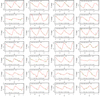 |
Fig. B.1. Examples of fitted templates for ACs light curves in the Y band. |
Appendix C: Comparison of relative zero points based on different extinction laws
Table C1 lists the coefficients of the PWJK for the LMC F mode and F+1O mode ACs obtained using different extinction laws (Wang & Chen 2023; Cardelli et al. 1989; Fitzpatrick 1999) and calibrated by adopting the geometric LMC distance as furnished by P19.
Comparison between PWJK relations in the LMC based on different extinction laws.
Appendix D: Determination of the average magnitude in J and Ks bands for Galactic Anomalous Cepheids
The identification of the Galactic AC sample was possible thanks to the OGLE IV and the Gaia surveys, resulting in 174 and 276 objects, respectively. From these surveys, we obtained periods and epochs of maximum and optical photometry in the Gaia bands. For the objects for which Gaia did not provide intensity-averaged magnitudes (see Ripepi et al. 2023), i.e. those only present in the OGLE IV catalog, we adopted the arithmetic mean published in the main Gaia source. Indeed, it has been shown that the Wesenheit magnitude in the Gaia bands calculated from the arithmetic mean does not differ significantly from that obtained from intensity-averaged magnitudes (e.g., Ripepi et al. 2022).
Concerning the NIR photometry, we only have a single-epoch photometry from the 2MASS (Two Micron All Sky Survey, Skrutskie et al. 2006) survey. Since this could lead to errors as large as 0.2 mag (depending on the amplitude of the AC light curves), we decided to use a standard template-fitting technique to obtain mean magnitudes in the J and Ks bands. In principle, the adopted technique is similar to that used in Section 3.2. However, in this case, we only have one epoch of observation from 2MASS. Therefore we cannot rescale the amplitude of the star using the observations themselves but instead, we have to assume fixed amplitude ratios in the J, Ks bands compared to amplitudes in the I or G bands, depending on the source of the data, i.e. OGLE IV or Gaia, respectively.
We determine the average amplitude ratios using the ACs in the LMC and SMC from our sample for which we have well-determined amplitudes in the J and Ks bands and optical amplitudes from OGLE IV and Gaia. We verified that the amplitude ratios remained constant for both F and 1O pulsators with no dependence on the period up to P∼1.8 days. The following equations list the different amplitude ratios in the various bands we adopted
 (D.1)
(D.1)
 (D.2)
(D.2)
 (D.3)
(D.3)
 (D.4)
(D.4)
In this way, from an amplitude in the optical band, we derived the amplitudes in the NIR bands. For each mode of pulsation, we used the template with a period closest to that of the analyzed star. Therefore for a given AC, the procedure foresees the following steps: i) use the period and epoch of maximum from OGLE IV or Gaia to calculate the phase of the single epoch 2MASS observation (only data with flag "AAA" were taken9); ii) rescale the amplitude of the assigned template using the appropriate quantity from Eqs. D.1 to D.4; iii) add a Δ Mag to the rescaled template until it overlaps with the 2MASS phased observation; iv) calculate the intensity-averaged magnitude of the template modified as described in the previous two points.
The error in the mean magnitude was calculated using a bootstrap technique, taking into account the uncertainty in the amplitude and the 2MASS magnitude. The mean magnitudes were then converted from the 2MASS photometric system to the VISTA one applying the transformations provided by González-Fernández et al. (2018). The final data sample is composed of 226 Galactic ACs (125 F and 101 1O mode, respectively). Through the R factor for fundamentalization calculated in Section 4.3, the MW ACs were studied as a unique sample.
Appendix E: Figures
The figures in this Appendix display the observed and fitted PL and PW relations for all other filters and filter combinations, and the comparison between the LMC and SMC PWJK and PWG relations.
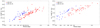 |
Fig. E.1. continued. |
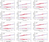 |
Fig. E.2. Relation fitting in different bands for ACs pulsators in the LMC. |
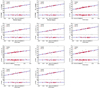 |
Fig. E.2. Continued. |
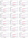 |
Fig. E.3. Continued. |
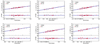 |
Fig. E.3. Continued. |
All Tables
Example of five epochs of the time series photometry for the star OGLE-SMC-ACEP-062 in the J band. The machine-readable version of the full table is available online at CDS.
Photometric parameters from the VMC survey for all the 198 LMC and SMC ACs analyzed in this paper.
Optical photometric parameters for all 198 LMC and SMC ACs analyzed in this paper.
Comparison between present results for ACs in the LMC, the SMC, and the literature.
Distances to the LMC without fixing the slope of the PW relations for the MW ACs.
Relative distances between the LMC and SMC, and the absolute SMC distance modulus calibrated through the LMC geometric distance modulus by P19.
Candidate ACs in GGCs. “Flag NIR” indicates the source of the NIR photometry, and “ID” lists the Gaia DR3 identification according to Gavras et al. (2023).
Draco distance moduli based on our PL and PW relations and Bhardwaj et al. (2024) NIR photometry.
Fourier parameters of the light curves templates in the Y band. The entire table is available electronically at the CDS.
Comparison between PWJK relations in the LMC based on different extinction laws.
All Figures
|
Fig. 1. Distribution of the AC data set in Magellanic Clouds. Red points are stars present in the VMC, while blue points are ACs from OGLE or Gaia with no VMC counterpart. The projection is a zenithal equidistant projection. The center is at RA = 55 deg, Dec = −73 deg. The empty black boxes show the footprint of the VMC survey. |
| In the text | |
|
Fig. 2. Number of epochs in the VMC Y, J, Ks bands for our AC sample. |
| In the text | |
|
Fig. 3. Examples of light curves (used to create templates) for different AC types. From the top: One 1O pulsator and one F pulsator in the Y (green), J (blue), and Ks (red) bands, respectively. We note that the photometric errors are smaller than the dot size, and the light curves have been doubled to shape them better. |
| In the text | |
|
Fig. 4. Templates created in every band: Y (top), J (middle), and Ks (bottom). |
| In the text | |
|
Fig. 5. Examples of template-fit AC light curves in the Y, J, and Ks bands (left to right columns). The green-filled circles are the observations, the red solid line is the best template for the light curve, and black-filled circles are the outliers not used in the fit. |
| In the text | |
|
Fig. 6. Period-luminosity relations in the NIR bands for the ACs in the LMC. Red and blue filled circles represent F and 1O mode ACs, respectively. We note that the error bars are smaller than the size of the dots. |
| In the text | |
|
Fig. 7. Example best fits for the F ACs in the LMC. From left to right, we show in the top panels the PLJ and the PLKs relations, and in the bottom panels, we show the PWJKs and the PWG relations, respectively. The red and gray filled circles are the data used for the fit and the outliers. The solid black line is the best fit to the data, while the dashed blue lines show the ±1σ levels. Upper panels and lower panels in each figure contain the fits and the residuals of the fit, respectively. The fits for the other bands are in the Appendix E. |
| In the text | |
|
Fig. 8. Example of fits for the F and 1O ACs in the LMC after 1O ACs were fundametalized by adding 0.145 to the logarithm of their periods. Each row contains two figures displayed in the left and right panels, respectively, in the following order: PLY, PLJ, PLKs, PWVI, PWVKs, PWG, PWYK, and PWJKs. For each figure, the upper subpanel shows the best-fitting line, while the lower subpanel reports the fit residuals. Red and blue filled circles represent the F and 1O mode ACs, respectively. The gray filled circles are outlier objects not included in the fit. The solid black line is the best fit to the data, while the dashed blue lines show the ±1σ levels. The best fits in additional bands can be found in Appendix E. |
| In the text | |
|
Fig. 9. From top to bottom: Dependency of the LMC PL relation zero point, slope, and dispersion, respectively, as a function of 1/wavelength. |
| In the text | |
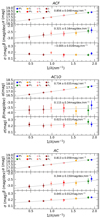 |
Fig. 10. Same as Fig. 9 but for the SMC. |
| In the text | |
|
Fig. 11. Distribution of the inferred LMC absolute distance moduli calibrated through Gaia DR3 MW AC parallaxes. The red histogram corresponds to the values obtained using MW AC parallaxes with no counter zero-point offset, while the red vertical line is the median of the distribution. The orange and blue histograms and vertical lines are the same as the red ones but were respectively derived using the counter zero-point offsets ϖZP = −0.014 mas, as suggested by Riess et al. (2021), and ϖZP = −0.022 mas, as suggested by Molinaro et al. (2023). |
| In the text | |
|
Fig. 12. Comparison between the LMC and SMC PWJK relation to determine the relative distances (see labels). In the top panel, red and blue filled circles are, respectively, the LMC and SMC F mode ACs, while the red and the blue solid lines are the fitted PL relations in the corresponding Cloud. In the middle panel, the green and yellow filled circles are respectively the LMC and SMC F mode ACs, while the green and the yellow solid lines are the fitted PL relations in the corresponding Cloud. In the bottom panel, the red filled and empty circles are respectively the LMC F mode and fundamentalized 1O mode ACs; blue filled and empty circles are respectively the SMC F mode and fundamentalized 1O mode ACs, while the red and the blue solid lines are the fitted PWJK relations in the corresponding Cloud. |
| In the text | |
|
Fig. 13. Position of the known and candidate ACs in GGCs from Cruz Reyes et al. (2025) in the PL and PW relations for ACs and T2Cs in the LMC. In the top panel, the green and blue lines are for the 1O mode and F mode ACs, and the magenta lines are for the T2Cs PLJ relations in the LMC, calibrated with the LMC distance modulus by Pietrzyński et al. (2019), respectively. Blue, orange, green, violet, brown, gray, light green, and cyan-filled circles are the known and candidate ACs in ωcen, Terzan1, NGC6752, NGC6388, NGC5466, NGC2808, M92, and M22. The middle and bottom panels show the same as for the top panel but for the PLKs and PWJKs relations, respectively. The NIR photometry for M92 is from Del Principe et al. (2005). |
| In the text | |
|
Fig. 14. Comparison of different Draco distance moduli. The reference values are taken from Stetson (1979), Nemec (1985), Aparicio et al. (2001), Bellazzini et al. (2002), Bonanos et al. (2004), Cioni & Habing (2005), Kinemuchi et al. (2008), Sesar et al. (2017), Hernitschek et al. (2019), Muraveva et al. (2020), Nagarajan et al. (2022), Bhardwaj et al. (2024). A red star shows the distance modulus to Draco obtained in the present work. |
| In the text | |
|
Fig. B.1. Examples of fitted templates for ACs light curves in the Y band. |
| In the text | |
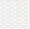 |
Fig. B.2. Same as for Figure B.1 but in the J band. |
| In the text | |
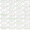 |
Fig. B.3. Same as for Figure B.1 but in the KS band. |
| In the text | |
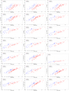 |
Fig. E.1. Same as Fig. 6 but for the remaining LMC and SMC PL and PW relations. |
| In the text | |
|
Fig. E.1. continued. |
| In the text | |
|
Fig. E.2. Relation fitting in different bands for ACs pulsators in the LMC. |
| In the text | |
|
Fig. E.2. Continued. |
| In the text | |
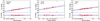 |
Fig. E.3. Same as Fig. E2, but for the SMC. |
| In the text | |
|
Fig. E.3. Continued. |
| In the text | |
|
Fig. E.3. Continued. |
| In the text | |
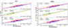 |
Fig. E.4. Same as in Fig.12 but for the PLK and PWG relations. |
| In the text | |
Current usage metrics show cumulative count of Article Views (full-text article views including HTML views, PDF and ePub downloads, according to the available data) and Abstracts Views on Vision4Press platform.
Data correspond to usage on the plateform after 2015. The current usage metrics is available 48-96 hours after online publication and is updated daily on week days.
Initial download of the metrics may take a while.