| Issue |
A&A
Volume 673, May 2023
|
|
|---|---|---|
| Article Number | A101 | |
| Number of page(s) | 21 | |
| Section | Interstellar and circumstellar matter | |
| DOI | https://doi.org/10.1051/0004-6361/202245200 | |
| Published online | 16 May 2023 | |
Aspect ratios of far-infrared and H I filaments in the diffuse interstellar medium at high Galactic latitudes
1
Argelander-Institut für Astronomie,
Auf dem Hügel 71,
53121
Bonn,
Germany
e-mail: This email address is being protected from spambots. You need JavaScript enabled to view it.
2
Tartu Observatory, University of Tartu,
61602
Tõravere, Tartumaa,
Estonia
e-mail: This email address is being protected from spambots. You need JavaScript enabled to view it.
Received:
12
October
2022
Accepted:
17
March
2023
Abstract
Context. Dusty magnetized structures observable in the far-infrared (FIR) at high Galactic latitudes are ubiquitous and found to be closely related to H I filaments with coherent velocity structures.
Aims. Considering dimensionless morphological characteristics based on Minkowski functionals, we determine the distribution of filamentarities ℱ and aspect ratios 𝒜 for these structures.
Methods. Our data are based on Planck FIR and HI4PI H I observations. Filaments have previously been extracted by applying the Hessian operator. We trace individual filamentary structures along the plane of the sky and determine 𝒜 and ℱ.
Results. Filaments in the diffuse interstellar medium (ISM) are seldom isolated structures, but are rather part of a network of filaments with a well-defined, continuous distribution in 𝒜 and ℱ. This distribution is self-replicating, and the merger or disruption of individual filamentary structures leads only to a repositioning of the filament in 𝒜 and ℱ without changing the course of the distribution.
Conclusions. FIR and H I filaments identified at high Galactic latitudes are a close match to model expectations for narrow filaments with approximately constant widths. This distribution is continuous without clear upper limits on the observed aspect ratios. Filaments are associated with enhanced column densities of CO-dark H2. Radial velocities along the filaments are coherent and mostly linear with typical dispersions of ∆υLSR = 5.24 km s−1. The magnetic field strength in the diffuse turbulent ISM scales with hydrogen volume density as B ∝ nH0.58. At high Galactic latitudes, we determine an average turbulent magnetic field strength of 〈δB〉 = 5.3 µG and an average mean strength of the magnetic field in the plane of the sky of 〈BPOS〉 = 4.4 µG.
Key words: ISM: clouds / dust, extinction / ISM: magnetic fields / ISM: structure / turbulence / magnetohydrodynamics (MHD)
© The Authors 2023
 Open Access article, published by EDP Sciences, under the terms of the Creative Commons Attribution License (https://creativecommons.org/licenses/by/4.0), which permits unrestricted use, distribution, and reproduction in any medium, provided the original work is properly cited.
This article is published in open access under the Subscribe to Open model. This email address is being protected from spambots. You need JavaScript enabled to view it. to support open access publication.
1 Introduction
A significant fraction of the interstellar medium (ISM) is filamentary. Predominantly within the last two decades, evidence has been accumulating from high-resolution all-sky surveys that the dust emission, stellar reddening, and H I line emission in large parts of the sky are correlated and shaped in filamentary structures. Moreover, it appears that ridges in the far-infrared (FIR) emission – observable with Planck at 857, 545, and 353 GHz – are aligned with the magnetic field measured on the structures (Planck Collaboration Int. XXXII 2016). Evidence for magnetically aligned H I fibers at high Galactic latitudes that extend for many degrees was found by Clark et al. (2014) based on observations with the Galactic Arecibo L-Band Feed Array survey (GALFA-H I Peek et al. 2018). Kalberla et al. (2016) used the HI4PI survey (HI4PI Collaboration 2016) to demonstrate that filamentary structures in H I are correlated with FIR emission at 353 GHz. Filamentary structures are also important in dense molecular gas regions, setting the initial conditions for star formation; see e.g. Hennebelle & Inutsuka (2019) and Hacar et al. (2022) for a recent reviews. Our investigations are restricted to the diffuse ISM with column densities NH ≲ 1021.7cm−2; gravitational instabilities are unexpected in this range and the magnetic field is in general aligned parallel to the filaments (Hennebelle & Inutsuka 2019).
Our current contribution is a follow-up to the work of Kalberla et al. (2021, Paper I), where we studied the coherence between FIR emission at 857 GHz and H I on angular scales of 18′. A Hessian analysis was applied to the large-scale FIR distribution observed with Planck, and to the H I observed with HI4PI. Such an analysis determines local maxima in the FIR and H I distributions from second-order partial derivatives. The data reveal that structures, or ridges, in the intensity map have counterparts in the Stokes Q and/or U maps. Upon tracing structures in orientation angles θ along the maxima, a tight agreement between FIR and H I was found in narrow velocity intervals of 1 km s−1. The FIR filaments are organized in coherent structures with well-defined radial velocities. Accordingly, radial velocities can be assigned to FIR filaments. Orientation angles 9 along the filaments – projected perpendicular to the line of sight – are fluctuating systematically. The derived distribution of filament curvatures was found to be characteristic for the distribution generated by a turbulent small-scale dynamo.
Here, we continue the analysis from Paper I, generating a complete census of filamentary structures in the diffuse ISM at high Galactic latitudes. Our intention is to provide observational constraints for aspect ratios of the fluctuation dynamo. To obtain better insight into the nature of filamentary structures, we use 2D Minkowski functionals. We trace individual structures and measure their surfaces and perimeters to derive their filamentarity. From an independent determination of the filament widths, we also derive aspect ratios of FIR/H I filaments for the first time and relate these to their filamentarities. For each individual structure, we also determine the average radial velocity and its dispersion. In Sect. 2, we give an overview of the observations and the data processing. Data analysis and results on the filamentarity of FIR/H I structures are presented in Sect. 3. We estimate the turbulent magnetic field strength in Sect. 4 and the mean field strength in the plane of the sky (POS) in Sect. 5. We then discuss our results in Sect. 6 and provide a summary in Sect. 7.
2 Observations and data processing
Our analysis is based on pre-processed data and results from Paper I. We used HI4PI H I observations (HI4PI Collaboration 2016), combining data from the Galactic all-sky survey (GASS; Kalberla & Haud 2015) measured with the Parkes radio telescope and the Effelsberg-Bonn H I Survey (EBHIS; Winkel et al. 2016) with data from the 100 m telescope. The H I data were correlated with FIR emission maps from the Public Data Release 4 (PR4; Planck Collaboration Int. LVII 2020) at frequencies of 857, 545, and 353 GHz1. The aim of the analysis of Paper I was to study the velocity-dependent coherence between FIR filaments at 857 GHz and H I; here we briefly describe their basic data processing.
2.1 Preliminaries: Hessian analysis
In Paper I, the Hessian operator H, which is based on partial derivatives of the intensity distribution, was used as a tool to classify structures as filament-like:
 (1)
(1)
Here x and y refer to the true angle approximations in longitude and latitude as defined in Sect. 4.1 of Górski et al. (2005). The second-order partial derivatives are Hxx = ∂2I/∂x2, Hxy = ∂2I/∂x∂y, Hyx = ∂2I/∂y∂x, and Hyy = ∂2I/∂y2.
The eigenvalues of H,
 (2)
(2)
describe the local curvature of H I and FIR features; λ_ < 0 is in the direction of least curvature and indicates filamentary structures or ridges. The 5 × 5 pixel matrix of the Hessian operator implies a spatial filtering that corresponds to a scale of 18′. Taking the resolution limits of the HI4PI survey into account, this is the highest possible spatial resolution that can be used to search the whole sky for filamentary FIR/H I structures. An adapted filtering was applied to improve sensitivity in the FIR; see Paper I for details.
The local orientation of filamentary structures relative to the Galactic plane is given by the angle
![Mathematical equation: $\theta = {1 \over 2}\arctan \,\,\left[ {{{{H_{xy}} + {H_{yx}}} \over {{H_{xx}} - {H_{yy}}}}} \right],$](/articles/aa/full_html/2023/05/aa45200-22/aa45200-22-eq4.png) (3)
(3)
in analogy to the relation
 (4)
(4)
which can be derived from polarimetric observations that provide the Stokes parameters U and Q.
The Hessian analysis, including the determination of local orientation angles along the filaments, was applied to FIR data at 857 GHz and repeated in H I for all velocity channels at |υLSR| < 50 km s−1. Applying an appropriate level λ_ < −1.5 Kdeg−2 at 857 GHz, a HEALPix bit map was derived that defines positions with significant filamentary structures. These data exceed an average signal-to-noise ratio (S/N) level of 68 at high Galactic latitudes. Positions with λ_ > −1.5 Kdeg−2 were flagged as undefined and excluded from the further analysis.
As the Hessian matrix operator was applied independently to all channels of the H I database, it is possible to consider velocity-dependent orientation angles Θ for the H I. Spurious structures from low-S/N data were excluded by applying an H I threshold of λ_ = −50 Kdeg−2. Each individual position that was previously determined to belong to a FIR filament was searched for the velocity with the best agreement in FIR and H I orientation angles. These velocities were encoded in a single nside = 1024 HEALPix database that is used for the current analysis. We emphasize that matching H I and FIR orientation angles locally (at individual positions, not within channel maps) allows us to measure random motions and velocity gradients along the filaments.
H I data with different velocity widths were considered in Paper I. The best correlation with typical alignment errors of 3° 1 was found for narrow velocity intervals of δυLSR = 1 km s−1. Velocities along the filaments are coherent but with typical fluctuations of ∆υLSR = 5.5 km s−1. A Gaussian analysis shows that the H I that is associated with the FIR filaments is cold with typical line widths of δυLSR = 3 km s−1, implying that the velocity fluctuations along the filaments are caused by supersonic turbulence. The FIR/H I correlation at latitudes |b| ≳ 20° is dominated by single narrow components belonging to the cold neutral medium (CNM). Broad lines from the warm neutral medium (WNM) have very little effect on the correlation. Blends from multiple independent CNM components may disqualify the data analysis that was described above. Fortunately, such blends from overlapping unrelated structures are rare at Galactic latitudes |b| ≳ 20° (see Sect. 3.1).
The dominance of the CNM within filaments that are exposed to supersonic turbulence has important consequences for the data analysis. Selecting channel maps at constant velocities with narrow velocity intervals as low as δυLSR = 3 km s−1 in the presence of velocity gradients and turbulent motions with ∆υLSR = 5.5 km s−1 leads to an artificial fragmentation of filamentary structures. Turbulent motions would partly shift structures to neighboring channels and the results depend on the selected velocity grid and the channel width. Broadening the velocity channels or using total column densities degrades the FIR-H I correlation (see Table 1 and Fig. 3 of Paper I). In addition, using a coarse velocity resolution implies limitations to the observed velocity coherence (see there Sect. 2.6 and Figs. 4 and 5) because filaments cannot be properly identified. Furthermore, the FIR–H I correlation with velocity coherence along the filaments cannot be generated by random processes from unrelated H I distributed along the line of sight. Such velocity caustics with prevailing density fluctuations in broad velocity intervals, predicted by Lazarian & Pogosyan (2000) and Lazarian & Yuen (2018), would be in conflict with our interpretation of three-dimensional density structures in the ISM.
2.2 Minkowski functionals and filamentarity
The aim of Paper I was to determine velocity coherence, local orientation angles, and the curvature distribution along the filaments. Here we restrict the analysis to the probability density distribution (PDF) of filamentary axis ratios. The easiest way to perform a parameterization is to consider aspect ratios 𝒜 = L/W by measuring the lengths L and widths W of filaments. A more general way is to consider geometrical descriptors for the morphology of filamentary structures in terms of Minkowski functionals. These functionals derive from the theory of convex sets and generalize curvature integrals over smooth surfaces. A fairly complete introduction to the basic morphological measures can be obtained from Mecke et al. (1994), Mecke & Stoyan (2000), and Kerscher (2000). Sahni et al. (1998) and Bharadwaj et al. (2000) apply Minkowski functionals to study the degree of filamentarity in the Las Campanas Redshift Survey.
In three dimensions, the four Minkowski functionals characterizing the morphology of a compact manifold are the volume V3D, the surface area S3D, the integrated mean curvature C3D, and the integrated Gaussian curvature G3D. These functionals can be used to define measures for the length L = C3D/4π, width W = S3D/C3D, and thickness T = 3V3D/S3D of objects under consideration. With a normalization L = W = T = r for a sphere of radius r, a spherical object would be characterized by L ≃ W ≃ T, a pancake as L ≃ W ⋙ T, a ribbon as L ⋙ W ⋙ T, and a filament as L ⋙ W ≃ T. Based on the three different length-measures L, W, and T, object shapes can be characterized with two dimensionless shapefinders: the planarity P = (W − T)/(W + T) and filamentarity F = (L − W)/(L + W).
Here, we are concerned with two dimensions: the thickness (hence also the planarity) cannot be measured but the filamentarity is still well defined. Bharadwaj et al. (2000) found it useful in this case to define the filamentarity ℱ by applying slightly different conventions, as mentioned above, using perimeter P and surface area S,
 (5)
(5)
By definition, 0 ≤ ℱ ≤ 1. We obtain ℱ = 0 for a filled circle and ℱ = 1 in the limit for a line segment of infinate length. As an example, and for a different shape, we mention ℱ = (4 − π)/(4 + π) ~ 0.12 for a filled square. Therefore, by calculating ℱ, it is possible to characterize the shape of an object with a single number and this is particularly useful if we want to quantify the extent to which the shape of an object can be described as a filament. Makarenko et al. (2015) applied this concept for the first time to characterize the shapes of H I cloud structures in the Milky Way.
2.2.1 Pixel counting
The Hessian analysis results in a HEALPix map with the best-fit radial velocities for each position on the filament. To determine P and S for individual structures, we need to trace the individual structures on this map. The surface area S can be determined simply by counting all the pixels nS that belong to the filament. For an nside=1024 HEALPix database, a single pixel covers an area of 4π/12 582 912 ~ 10−6 sr or 3.3 × 10⁻³deg2. The perimeter P can be determined in several ways using the Cauchy-Crofton formula (Legland et al. 2011). However, we are faced with a time-critical computational problem (Lehmann & Legland 2012): we need to analyze 5.4 × 10⁶ boundary pixels. We decided to solve this by pixel counting in two ways, counting pixels nPout just outside the structure, and alternatively counting pixels nPin along the rim, but inside it; using the average of the two counts approximates the set of curves that can go through adjacent regions; see Fig. 2c of Stawiaski et al. (2007). In addition, for each position inside the filament, we determine the number of nearest neighbors nNeighbor that are also inside. The HEALPix tessellation allows up to eight neighbors2. Positions with nNeighbor = 8 can be considered as deep inside the filament.
2.2.2 Simulations
A basic check for numerical applications of Eq. (5) is to ensure that the calculations result in ℱ = 0 for a filled circle. Bharadwaj et al. (2000) notice a further simple relation that allows us to test the accuracy of calculating ℱ for filamentary structures. The region between two concentric circles with radii R2 < R1 has a filamentarity of
 (6)
(6)
To test our numerical procedure, we generated an nside=1024 HEALPix database, first defining a filled circular disk centered on the Galactic plane with a radius of r = 25°. We then generated a series of pseudo-filaments, that is, regions between two concentric circles at radii R1 = r + δr and R2 = r − <δr. These simulate filaments with widths of 2δr, surfaces of  , and perimeters of 2π(R1 + R2). The filamentarity can be determined according to Eq. (6).
The direct numerical application of Eq. (5), using PPout or PPin to determine the perimeter and nS to determine the surface led immediately to an inconsistent result, namely ℱ = 0.25 for the filled circle. Equation (5) is defined for the ideal case of a distribution that can be represented with continuous contours. Bharadwaj et al. (2000) pointed out that this definition should be modified for data on a grid. These authors propose different shapefinder versions for a rectangular grid. However, using the version with their Eq. (6) leads only to a slight improvement, that is, ℱ1 = 0.13 for the filled circle. Next we tested another shapefinder relation according to Eq. (8) of Bharadwaj et al. (2000) and found that with ℱ2 = 0.23 for the filled circle, this relation is also not appropriate for our application.
We decided to continue along the definition in Eq. (5) but to consider the properties of the HEALPix database in detail. The HEALPix tessellation provides the same surface area for all pixels but slightly different shapes (Górski et al. 2005). The surface is therefore well defined when counting pixels nS inside the filament, but the HEALPix grid is variable, locally approximating a rectilinear equal-area grid that is rotated against the Galactic coordinate system by 45° (Górski et al. 2005, Figs. 4 and 5). The direction weights for rectangular grids that are needed for the Crofton formula in discrete images (Lehmann & Legland 2012, Fig. 1) are position dependent, which implies that distances between individual pixels along the perimeter of a filament are variable. Direct distance measures along jagged filament borders using nPout or nPin are biased in any case. We take this into account by applying an average correction using a bias factor fb, such that the outer and inner perimeters are approximated by PPout = nPoutfb or PPin = nPin fb, respectively.
Generating a series of pseudo-filaments at a constant radius of 25ºwith variable widths 2δr, we calculated the expected filamentarity ℱmodel according to Eq. (6) and varied the geometric correction factor fb. From about 3600 model calculations, the best fit with ℱ/ℱmodel = 1.00005 ± 1. × 10−3 was found for fb, = 0.773. For the filled circle, we determine in this case ℱ = −1.16 × 10⁻³, and also the minimal deviation from zero that we found during the simulations. We emphasize that the correction with a factor fb, = 0.77 is a statistical correction only. The simulations described above used a well-defined test bed with a uniform distribution of orientation angles. We expect that the correction factor fb = 0.77 is unbiased, but the application to complex filamentary structures is probably far less accurate than the average 0.1% error level that could be achieved during the simulations. In any case, measurements of the perimeters of pix-elized structures always come with uncertainties, which depend on the size and orientation of the object. Using computationally more elaborate Crofton methods, one would expect relative errors of up to 1 or 5% depending on the algorithm used; see Fig. 5 of Lehmann & Legland (2012).
We like to note here that outer and inner perimeter counts show only minor deviations as long as the filaments are extended and well defined (as in the simulations). For short filaments, significant differences are notable and we therefore use the average P = fb (nPout + nPin)/2 as the best estimate for the perimeter. Perimeters around surfaces with ns < 10 are ill defined. From Fig. 4 of Lehmann & Legland (2012), we expect that errors, which are independent of the numerical method used, would exceed 20% in these cases. Such objects are disregarded.
Our simulations were also used to estimate the filament widths, which are defined as the average width along the filament. For a filament with a simple geometry one would first determine the skeleton (or center) of the filament and measure – for each position along the skeleton – the width perpendicular to the direction defined by neighboring skeleton elements. This procedure can become complicated when faced with complex filament geometries or filament branching, with ambiguities at sharp turns.
We used a different method that is independent of filament shape. For each pixel inside the filament, we counted the number of neighbors nNeighbor We then determined the average neighbor count CNeighbor = Σ nNeighbor/ns· During our simulations, we tabulated CNeighbor as function of the filament widths W known from the model. This table is later used to infer the average widths W from the CNeighbor counts; Fig. 1 shows the calibration curve. This method was found to produce robust results up to a width of 10 pixels. We show below that we only need to consider filaments with an average width of up to 5.5 pixels. The width counts W measures average distances (corrected for geometrical sampling effects by application of the factor fb, = 0.77), for an nside = 1024 HEALPix database in units of 10−3 rad or 5.7 × 10⁻² deg.
In closing this section, we need to point out that the path from the theoretical definition of filamentarity in Eq. (5) to a meaningful derivation of parameters is hampered by a number of uncertainties. Naive methods for the surface, perimeter, and width determination can lead to huge systematic errors (Lehmann & Legland 2012). Our numerical recipes are valid for filamentary objects with a uniform distribution of orientation angles and have been tested against objects with known filamentarity and width. It is impossible to estimate uncertainties in cases of observed filament geometries, which can be highly complex and variable. We therefore refer to Sect. 3.3, where we compare derived aspect ratios and filamentarities with the expected model distribution. Uncertainties and systematical errors should show up in this instance.
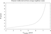 |
Fig. 1 Average filament widths derived from neighbor counts during simulations. |
3 Data analysis and results
Using the results from the Hessian analysis in Paper I, we trace whether or not each position of the nside = 1024 HEALPix database is part of a filament. For each position inside a filament, we determine the number of neighbors nNeighbor By tracing individual filamentary structures, we calculate surface S, perimeter P, average width W, and average position in Galactic coordinates. We also calculate the average radial velocity υLSR with the associated dispersion Δυ along the filaments. In Sect. 4.2, we use distances to the wall of the magnetized Local Bubble (LB) from dust data modeled by Pelgrims et al. (2020) and determine average filament distances, assuming that these might be associated with the LB wall4.
3.1 Limitations: confusion in the Galactic plane
To study the global distribution of filaments in the Milky Way, we first show the latitude distribution of filament widths W in Fig. 2. At high Galactic latitudes, the derived widths are typically in the range of 1.5 ≲ W ≲ 4.5 pixels. However, approaching the Galactic plane, we find that W becomes strongly biased, up to W ~ 10. This distribution is caused by confusion. Numerous filaments overlay each other at velocities −50 < υLSR < 50 km s−1 and appear as one in projection. This leads to spurious structures that cannot be reasonably interpreted with our current approach. The low latitude bias is not unexpected, because the analysis in Paper I focused on high latitudes. We also note that all spurious structures in the Galactic plane have huge surfaces.
Inspecting the results of our analysis, we find that large filaments at latitudes |b| ≳ 30° extend to somewhat less than 20 000 pixels, and those at low latitudes to far larger dimensions, propagating in position to lower latitudes. As an example, for a reliable filament extraction, we mention the structure at l = 44°.1, b = 41°.1, which is discussed later in Sect. 3.6, with a surface of nS = 18 563 pixels. Extrapolating this result, we use a fiducial upper limit of nS = 20 000 pixels for the analysis of filamentary structures, corresponding to 0.02 sr or 65.6 deg2. Such extended structures are not traced for further extensions and are also eliminated from the statistical analysis. This simple recipe has proven to be quite successful, because it allows the user to eliminate all structures that show obvious signs of originating from blending. At the same time, features with a width of W ≳ 5.5 are removed. The final constraint for our analysis is that surfaces must be in the range of 10 < nS< 20 000 pixels. This restriction leads to a total number of 6568 filaments that can be used for our analysis.
Our constraint of nS < 20 000 is somewhat arbitrary; we experimented with limits in the range 15 000 < nS < 20 000 and found that our results are not significantly affected by a particular choice. However, a limit of this kind turned out to be very useful in identifying H I regions that are affected by confusion. Using the Gaussian decomposition from Paper I, we compared the best-fit H I velocity for each filament position (from matching FIR/H I orientation angles) with the center velocities of the Gaussian components. We selected the nearest component in velocity at υnear and also – independently – the dominant component with the largest column density in the spectrum at υdominant· Assuming that the FIR/H I correlation in orientation angles from Paper I is caused by H I density enhancements, both selections may point to H I counterparts of the FIR filaments. For filaments with nS < 20 000, we find that in 25% of all cases, identical components are selected. Component velocities deviate in 66% of all cases by ∆υGauss = |υnear − υdominant| < 5.5 km s−1, which is equal to the velocity dispersion along the filaments determined in Paper I. Figure 3 shows the cumulative distribution function (CDF) for the occurrence of a component separation, ∆υGauss. In comparison to a normal distribution with a velocity dispersion of 5.5 km s−1, we find a clear observational preference for component separations of ∆υGauss < 5.5 km s−1. The CDF for filaments with nS > 20 000 is for all ∆υGauss values significantly below the selection with nS < 20 000.
Figure 4 shows the sky distribution of FIR/H I filaments for the selection nS < 20 000 that is used in the following. As opposed to the distribution shown in Fig. 1 of Paper I, most of the filamentary structures at Galactic latitudes |b| ≲ 20° are excluded because of confusion. Such a selection is consistent with the empirical assumption shared by many observers that only the range |b| ≲ 20° may be considered as “high Galactic latitudes", and therefore unperturbed by confusion.
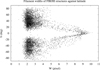 |
Fig. 2 Spatial distribution of filaments with width W as function of latitude b. |
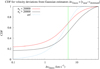 |
Fig. 3 Cumulative distribution function of velocity separations ΔυGauss = |υnear − υdominant| between Gaussian components associated with H I filaments that are nearest in velocity and dominant in column density. |
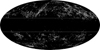 |
Fig. 4 Distribution of the 6568 FIR/H I filaments in Mollweide projection. The horizontal lines indicate Galactic latitudes of b = 20° and b = −20°. |
3.2 Filament widths
Figure 5 displays the spatial distribution of the filaments with their derived widths after constraining the surface area. On average, we find a width of 2.53 pixels. For a single pixel in a nside = 1024 HEALPix database, the angular resolution is Θpix = 3′.44 (Górski et al. 2005). Assuming filament distances of 100 pc (Sfeir et al. 1999), we estimate an average filament width of 0.25 pc.
We find that the average filament widths increase with the filament surfaces, W = 0.74 + .01 + (0.491 + .004)ln(nS). The data and fit5 are shown in Fig. 6. Stripy structures in this plot come from the fact that nS as a pixel sum is an integer number, while averages over pixel counts can be treated as real numbers. Also, perimeter counts are, by definition, quantized and some of the later presentations are affected by integer arithmetic due to pixel counts. The Hessian operator is selective and most sensitive to FIR/H I data with local S/N maxima (constant multiple rule). This implies that prominent ridges have stronger eigenvalues −λ−, and therefore the average filament widths W increase depending on the significance level λ− < −1.5 Kdeg−2 at 857 GHz. This effect is reproduced in Fig. 7 and discussed in Sect. 3.3 in more detail. We interpret such structures with enhanced column densities in gas and dust.
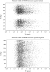 |
Fig. 5 Spatial distribution of filaments with width W for 10 < nS < 20 000, as a function of latitude b (top) and longitude l (bottom). |
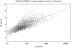 |
Fig. 6 Average filament width W as a function of filament surface, measured by counting surface pixels nS. The red line represents the fit W = 0.74 ± .01 + (0.491 ± .004)ln(nS) |
3.3 Filamentarity and aspect ratios
For each of the 6568 structures, we calculate the filamentarity ℱ according to Eq. (5) by determining the pixel counts nS for the surfaces S within the filaments. The perimeters are derived from the average of the inner and outer pixel counts along the rims of the filaments by applying the correction factor fb, as determined in Sect. 2.2.2, that is, P = (PPout + PPin)/2 = fb(nPout + nPin)/2.
The distribution of the resulting filamentarities as a function of the surface pixel count nS is shown in Fig. 8 together with two simple filamentarity models. The first model (blue dashed line) assumes a common width of W = 2.53 pixels. For the second model (red line), we use the fit W = 0.74 + 0.491 ln(S). This model shows obvious improvements for large surfaces, and we use it in the following. We find a rather homogeneous and continuous distribution that covers three orders of magnitude in surface. The scatter can be explained by the uncertainties in the parameter determination. Most significant is the statistical error  in the perimeter determination. Neglecting independent errors in W, we estimate 3σ uncertainties, which are plotted with dash-dotted orange lines in Fig. 8. Outliers can be traced back to filaments with large widths in Fig. 6. We find no evidence for other systematical biases.
Aspect ratios are usually estimated visually as 𝒜 = L/W from the measured filament lengths L and widths W. Here, we generalize this concept. The filamentarity ℱ, which depends on the Minkowski functionals P and S only, is sensitive to the shape of a structure, but not to its size; it is further invariant against translation or rotation and describes the filamentary shape of a class of objects whenever the P and S values lead to the same value ℱ defined by Eq. (5). In a similar way, we may consider all objects with the same L/W ratio as equivalent. Filamentarity and aspect ratio can then be linked. First, we generalize the length as L = P/ 2 and obtain
 (7)
(7)
The top panel of Fig. 9 shows the relation between ℱ and 𝒜 for all of our objects, using independent determinations of surface S, perimeter P, and average width W. For the lower plot, we use the relation W = 0.74 + 0.491 l·n(nS) from Fig. 6 to estimate the width from the surface. This statistical estimate can be compared with the measurements. In case of independent measures for P and W (Fig. 9 top), we obtain a very tight and clean relation between ℱ and 𝒜, suggesting a close relation of W = 2S/P for the filaments, and therefore
 (8)
(8)
and we obtain the 𝒜-to-ℱ relation,
 (9)
(9)
A low filamentarity observed for an isolated structure must be formally considered as an indication that this structure does not represent a filament. The implication of Fig. 9 is that low filamentarity may not in all cases be interpreted this way. Our sample needs to be considered as a homogeneous class of objects. Short filaments with low aspect ratios are characterized by a low filamentarity but these objects do not separate from the sample shown in Fig. 9. Objects belonging to this low end of the filament distribution may suffer from observational uncertainties, in some cases even leading to negative filamentarities, but are definitively part of the filament population. It is remarkable that the upper plot in Fig. 9 with aspect ratios from Eq. (8) shows less scatter than the plot below with the W fit described in Sect. 3.2. This means that the individually measured filament widths W are well defined, and a significant fraction of the scatter in the top panel of Fig. 6 must reflect filament properties.
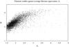 |
Fig. 7 Average filament width W as a function of the average Hessian eigenvalue −λ− from 857 GHz data. |
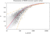 |
Fig. 8 Filamentarity of 6568 structures as a function of filament surface measured by counting filament surface pixels nS. The dashed blue line shows a model of the filamentarity in the case of a constant width of W = 2.53 pixels, and the red line shows the model for the broadening fit from Fig. 6. Formal numerical 3σ uncertainties from perimeter counts are indicated by the dash-dotted orange lines. |
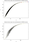 |
Fig. 9 Distribution of filaments covering the parameter space in aspect ratio 𝒜 and filamentarity ℱ. The distribution in the top panel was derived using the width W as described in Sect. 2.2.2 for each filament. For the distribution in the bottom panel, we use widths as determined from the fit described in Sect. 3.2. The dashed yellow line is derived from Eq. (9) using aspect ratios according to Eq. (7). Positions marked in red in the upper plot belong to the two filaments described in Sect. 3.6; merging these filaments results in a single structure, marked with blue. |
3.4 Probability density distributions
So far we have considered predominantly the distribution of filamentarities and aspect ratios for individual structures. Here, we focus also on the total surface covered by filaments, which is characterized by ΣnS, the sum over all filaments in a given range.
3.4.1 Filamentarity
Figure 10 shows that the PDF of filamentarity by number is fundamentally different from that obtained from the distribution obtained by weighting with the total surface of the filaments. The upper part of Fig. 10 may be compared with the PDF derived by Makarenko et al. (2015, Fig. 7). These authors considered isocontours of the fluctuations in the gas number density obtained from the H I distribution at a constant galactocentric radius of 16 kpc, obtaining a peak of the PDF at ℱ ~ 0.15 with a power-law tail at larger values with a truncation at ℱ ~ 0.75. Their distribution resembles that of triaxial ellipsoids and Makarenko et al. (2015) argue that the form of their PDF indicates that the H I distribution is indeed filamentary in 3D but truncated at an aspect ratio of length/thickness of about 20. In an extensive analysis, Soler et al. (2020, 2022) studied the filamentary structure in atomic hydrogen emission toward the Galactic plane and confirmed that a significant fraction of the H I distribution is in filaments; however, these authors did not determine aspect ratios or filamentarity.
We do not observe a truncation at high ℱ values, and the weighted PDF of filament surfaces, displayed in the bottom panel of Fig. 10, shows rising surfaces for increasing ℱ. Filaments with values ℱ ≳ 0.9 contribute significantly to the total surface covered by the filamentary H I and FIR distribution. We note that filaments with surfaces of nS > 20 000 pixels are excluded and do not contribute to Fig. 10.
3.4.2 Aspect ratio
Figure 11 presents the PDFs for the aspect ratios for comparison. Most of the analyzed filamentary structures have low aspect ratios. The distribution is continuous, at least up to 𝒜 ~ 125. The PDF of filament surfaces indicates that even aspect ratios of 200 ≲ 𝒜 ≲ 600 exist, but these contribute less to the PDF at the bottom of Fig. 11, which is weighted by surface. The exclusion of filaments with surfaces of nS > 20 000 pixels implies that large aspect ratios are under-represented because of confusion limitations. Our results deviate significantly from those of Makarenko et al. (2015), who considered H I cloud complexes in the Galactic plane at a constant galactocentric radius of 16 kpc and found only moderate aspect ratios.
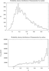 |
Fig. 10 Probability density distributions of filamentarities ℱ. Top: distribution by number. Bottom: distribution weighted by the total surface covered by filaments. |
3.5 Velocity coherence revisited
One of the most striking results from the analysis in Paper I is that FIR filaments at 857 GHz are associated with H I at well-defined radial velocities. Paying attention to the constraints discussed in Sect. 2.1, it is possible to assign radial velocities to the FIR filaments. The average velocity dispersion along the filaments is defined in Sect. 2.6 of Paper I from a two-point function within a radius of 1o. Velocity fluctuations of ∆υLSR ~ 5.5 km s−1 along the filaments were found to be representative for turbulent motions within the ISM. Some strong velocity deviations – exceeding the expected three-sigma limit for a normal distribution – are found from visual inspection but such deviations appear not to disrupt the filamentary structure. As opposed to Paper I, we wish to consider here individual filaments. Having extracted these, we intend to check whether the velocity coherence is constrained by the filamentarity of the structures. First, we determine the average radial velocity of each filament, followed by the standard deviation of the velocity fluctuations along the filament.
In the top panel of Fig. 12, we plot the average radial velocities of the filaments and below the corresponding velocity dispersions as a function of aspect ratio. The largest scatter in radial velocity and associated velocity dispersion exists for 𝒜 ≲ 20. A fraction of the filaments at velocities υLSR ≲ −20 km s−1 can be attributed to intermediate-velocity clouds (IVCs) with low velocity dispersions. The radial velocities of the filaments are mostly close to zero for large aspect ratios, implying that these filaments must be predominantly local. The average velocity dispersion for our sample of filaments is ∆υLSR = 5.24 km s−1. While this dispersion may be considered as representative for internal turbulent motions within the filaments, a slight increase for large filaments can be caused by velocity gradients along the filaments. Larger surfaces imply larger aspect ratios. The dispersions in Fig. 12 appear to increase slightly with aspect ratio, but this impression is biased by low dispersions from IVCs at low aspect ratios; the correlation coefficient is 0.08. In a similar way, the correlation coefficient between velocity dispersion and surface is 0.06. There is no clear evidence that large filaments must also have large velocity dispersions.
Outliers, which are defined at positions with velocities that deviate from the average filament velocity by more than three times the velocity dispersion, may be caused by statistical uncertainties, by turbulence-driven deviations, or alternatively by systematic effects, indicating blending from unrelated structures. We define the outlier fraction O as the fraction of positions with outliers relative to the number of positions of the total filament surface. Figure 13 shows this outlier fraction as a function of filament surface nS. The presentation is dominated by integer arithmetic, from bottom up with outlier counts of zero, one, two, and so on. There is no evidence that filaments with large surfaces nS suffer from a large outlier fraction. The blue vertical line in Fig. 13 divides the filament distribution at nS = 500 in two samples containing approximately the same total column density. We use this threshold in the following analysis to distinguish filaments that, visually, appear to be prominent (for nS ≳ 500) from those appearing less prominent (nS ≲ 500). Prominent structures appear to be less affected by outliers. Figure 14 shows that the outlier fraction is largest at positions that are less significant and have low average Hessian eigenvalues −λ−. Filaments were defined in Paper I according to FIR distribution, and the radial velocities were then determined by matching H I structures. We conclude that most of the velocity outliers are probably caused by sensitivity limitations. Visual inspection shows many cases of outliers along continuous structures on small scales. At high Galactic latitudes, we find no direct evidence that a significant number of outliers is caused by confusion with unrelated structures. Filament positions are derived from the Hessian analysis of the FIR at 857 GHz. We use the H I data to determine the velocity field but we do not flag FIR filament positions as invalid in the case of outliers.
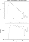 |
Fig. 11 Probability density distributions of aspect ratios 𝒜. Top: distribution by number. Bottom: distribution weighted by the total surface covered by filaments. |
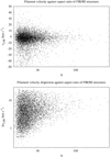 |
Fig. 12 Velocity distribution as a function of aspect ratio. Top: average filament H I radial velocities. Bottom: velocity dispersions within the filaments. |
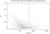 |
Fig. 13 Fraction O of outlier positions depending on filament surface nS. Outliers are defined as positions with velocities deviating from the average filament velocity by more than three times the velocity dispersion. The presentation is strongly quantized, showing, from bottom to top, outlier counts of zero, one, two, and so on. The blue vertical line divides the sample at nS = 500. |
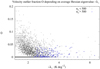 |
Fig. 14 Fraction O of outlier positions as a function of the average Hessian eigenvalue −λ− from the FIR data. Blue data points are from prominent filaments with nS > 500. |
3.6 A network of filaments
Filaments do not only exist as distinct, thin elongated structures; they appear also as part of an extended network. To enable the presentation of individual filamentary structures, we extracted two such filamentary networks that contain elongated features, which are shown in the top panel of Fig. 15. The color coding shows the number of neighbors nNeighbor that are used to characterize the thickness of the filament. Boundary pixels nPout just outside the filaments are shown in blue. The display appears to show a single structure but a closer look at the lower structure in latitude shows that this filament is disconnected. Two of the boundary pixels touch each other, giving the impression of a connection.
The northern filament covers a surface of 13 198 pixels, resulting in a width of W = 4.4 in 𝒜 = 637, ℱ = 0.9897. Velocities are centered on υLSR = −9.4 km s−1 with a dispersion of ∆υLSR = 11.7 km s−1. For the southern part, we measure nS = 1967, W = 3.6, 𝒜 = 145, ℱ = 0.9553, υLSR = −14.4 km s−1, and ∆υLSR = 10.7 km s−1, respectively. The filament velocity field is shown in the lower part of Fig. 15, including other structures in the vicinity. Some of the smaller fragments appear to be aligned with larger filaments, suggesting a common flow. The color code allows us to estimate velocity gradients; in most cases these show smooth transitions but there are rapid changes in a few cases.
Surprisingly, concerning the characterization of filaments as being located on the 𝒜-to-ℱ track (Fig. 9 and Eq. (9)), whether or not these two filaments are connected is irrelevant. The filaments are part of a hierarchy of filaments, defined by 𝒜-to-ℱ relation. Coalescence or breaking of filamentary structures leads to a repositioning of the filament positions along the 𝒜-to-ℱ track shown in Fig. 9. This can be demonstrated in the case of the filaments shown in Fig. 15. We indicate the positions of the two observed filaments with red markers in the 𝒜-to-ℱ plot in the top panel of Fig. 9. Merging both filaments replaces these entries with a new one on the 𝒜-to-ℱ track indicated in blue. In general, merger or disruption of filaments leads to a repositioning of structures on the path defined by Eq. (9) but these structures do not leave the 𝒜-to-ℱ track. Thus, the distribution is self-replicating. This property mitigates the observational limitations to some extent. Sensitivity limitations imply that we are limited in our analysis to the strongest features; there are likely to be many more, weaker features. As long as observational gaps due to sensitivity limitations are not too large, we expect the 𝒜-to-ℱ distribution (Fig. 9, top) to be representative.
As pointed out by Mecke et al. (1994), Minkowski functionals are global and additive measures (see their Eq. (12)). Additivity allows us to calculate these measures by summing up local contributions, as in our example. We also note that filaments that are affected by projection effects remain on the 𝒜-to-ℱ track as long as the measured filament width W remains unaffected. The aspect ratio is largest for filaments that are oriented perpendicular to the line of sight. Assuming for example a simple linear structure, a rod. Tilting such a filament by an angle θPOS against the plane of the sky reduces S and P by the same factor of cos (θPOS); this also modifies the aspect ratio but also affects ℱ− according to Eq. (9) – such that the filament stays on the 𝒜-to-ℱ track. The additivity property of Minkowski functionals allows us to generalize this simple example in the case of complex structures by considering a piece-wise decomposition in local structures with subsequent addition. However, an observational difficulty is that, with increasing misalignment, it becomes increasingly difficult to accurately determine surface, perimeter, and width. We relate some of the scatter for low aspect ratios in Fig. 9 to observational uncertainties of this kind and note that, during our simulations (Sect. 2.2.2), inaccuracies in the width determination were found to be most critical at low aspect ratios. As a counter example, objects with large planarity (pancakes) may appear in projection as filaments. For an isotropic distribution, members of this class should also appear as circular structures in the plane of the sky with ℱ ~ 0. This is not observed within the uncertainties shown in Fig. 8.
Figure 16 shows another prominent and well-defined filamentary network at high Galactic latitudes. We determine in this case nS = 18 563, W = 4.7, 𝒜 = 787, ℱ = 0.9917, and υLSR = −0.4 km s−1 with ΔυLSR = 8 km s−1. In comparison to Fig. 15, we find less pronounced linear structures but more branches and loops.
We close this subsection with an example of a complex, confusion-limited structure that we excluded from our analysis. This structure, shown in Fig. 17, is the famous dusty filament6, aligned with the galaxy’s magnetic field in the foreground of the Magellanic clouds (Planck Collaboration Int. XXXII 2016, Figs. 4 and 18). Albeit a prime example of a filament, it cannot be separated from the complex northern part of the H I distribution, which appears to be strongly blended. During data processing, this structure was truncated automatically after reaching a limit of nS > 20 000 (see Sect. 3.1). In this case, we determine formal parameters of W = 5.2, 𝒜 = 706, ℱ = 0.9906, and υLSR = 4.7 km s−1 with ∆υLSR = 5.7 km s−1. These parameters are consistent with those of other filaments but we emphasize that this outstanding source did not enter our statistics.
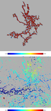 |
Fig. 15 Spatial distribution of filamentary structures in gnomonic projection. The field size is 27°.7. Top: isolated filamentary structures discussed in the text. For each position, the color coding shows weights according to the number of neighbors nNeighbor inside the filament. Boundary pixels nPout just outside the filaments have weight −1 and are coded in blue. Bottom: velocity field of the filamentary structures, including all other filaments in the field. The center position is l = 260°, b = 58°. |
3.7 The dark connection
Associated with the FIR distribution at 857 GHz are filamentary H I structures that are considerably colder than the surrounding ISM (Paper I). Adopting the hypothesis of a constant E(B − V)/NH ratio, Kalberla et al. (2020) suggested that these structures must be associated with CO-dark molecular hydrogen. We use column densities in NH and NH2 determined by these authors. To test whether there might be an enhancement of the total hydrogen column densities NH within the filaments, we first calculated the pixel-based average hydrogen column density NHoff for all positions that are not covered by FIR filaments. To take spatial fluctuations of NHoff into account, we generated an average distribution  on an nside = 128 HEALPix grid, implying a spatial averaging over a pixel size of 27′.5. We then determined the average column density
  for each filament and the average
  for the center positions with nNeighbor = 8, separately. The ratios
  and
and  can be used to characterize an excess in hydrogen column density.
Summarizing over all filaments from our sample, we determine  (1.71) and
  (1.86). These calculations can be repeated using the CO-dark H2 content. The average H2 excess in filaments is in this case 4.32 (5.60) and 5.29 (6.67), respectively. The values in brackets are obtained when only prominent filaments are selected and indicate a further increase of ~23%. Figure 18 confirms the trend that prominent filaments with nS > 500 tend to have a larger NH excess. Figure 19 shows the latitude dependence of the NH excess. There is no significant dependence on Galactic latitude (or on longitude, but not shown); most of the NH-excess is contained within filaments with large aspect ratios or surfaces. The H2 distribution caused by condensations in the colder part of the CNM is strongly organized in filaments (see Fig. 11 of Kalberla et al. 2020).
In principle, dependencies between column densities and aspect ratios can be used to infer the extent to which filaments are tilted away from the plane of the sky. The aspect ratio is in this case reduced by a factor cos (θPOS), but the total column density of the filament remains constant. The apparent surface also decreases by a factor of cos (θPOS) and we should observe an average column density excess for low aspect ratios; however, this is not observed. On the contrary, Fig. 18 indicates a weak tendency – with a correlation coefficient of 0.34 – for an increase in the column density excess with increasing aspect ratio, hence with increasing surface.
Figure 20 shows that there is also a weak correlation between NH column density excess and width, with a coefficient of 0.36. We conclude that denser FIR/H I filaments tend to have an increased width W. This tendency cannot be explained by projection effects. We note in Sect. 3.2 that filament width increases with total filament surface area (Fig. 6), and also that the filamentarity is affected by an increase in W (Sect. 3.3 and Fig. 8). Figure 7 indicates that such structures tend to have a high significance level −λ−. Consolidating this information, prominent filaments tend to have increased width and to be associated with NH enhancements, and it is tempting to speculate that such filaments may also be associated with stronger magnetic fields.
We do not know the extent to which projection effects have led to enhancements in the observed hydrogen column densities. However, the additional increase in the filament centers cannot be explained by mere projection effects. The observed effects are relatively strong in comparison to the results by Koch & Rosolowsky (2015), who obtain enhancements in brightness temperature by a factor of 1.3 for filaments in the Herschel Gould Belt Survey. We conclude that FIR filaments in the diffuse ISM are associated with cold H I gas and CO-dark molecular hydrogen that is concentrated toward the filament centers.
For a complete evaluation of the distribution of hydrogen column densities in filaments, we calculated the total column density content NHtot for each individual filament. Figure 21 shows that the FIR/H I filaments are part of a well-defined homogeneous population of structures. For the filament length L = P/2, we fit NHtot ∝ (P/2)1.35 and for the surface  . Assuming that filaments at different scales effectively sample similar gas densities in the ISM, we expect an increase of NHtot ∝ nS. The observed enhancement of NHtot at large surfaces is consistent with the increase in W for large surfaces, also with increasing eigenvalues −λ− (Sect. 3.2), implying stronger FIR/H I ridges. The NHtot distribution is partly self-replicating, and merger or disruption of individual filamentary structures leads to a repositioning of the filaments within the distribution of Fig. 21. Projection effects decrease the projected surface without changing NHtot and therefore cause an increase in the observed scatter. Hacar et al. (2022) relate the mass M in filaments to their length L and find that the entire distribution of filaments (except H I filaments) roughly follows the distribution L ∝ M1/2. Figure 21 top is incompatible with such a distribution.
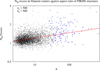 |
Fig. 18 Excess in total hydrogen column density |


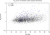 |
Fig. 19 Excess in total hydrogen column density |

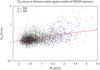 |
Fig. 20 Excess in total hydrogen column density |


3.8 Fractals: the surface-perimeter relation
Filaments represent hierarchical configurations with spatial structures on all scales. According to Mandelbrot (1982), self-similar structures are ubiquitous in nature and are often linked to a fractal geometry, which characterizes the self-similar scaling of surface structures. Mandelbrot et al. (1984) define the fractal dimension D (sometimes referred to as the Hausdorff dimension) with the surface-perimeter relation P ∝ S D/2. Here, D can range from circular sources with D = 1 to highly convoluted structures with D = 2. In an extensive analysis, Falgarone et al. (1991) applied this approach to molecular cloud structures in the range 0.1–100 pc. These authors obtained a common fractal dimension D = 1.36 + 0.02 independent of the different scales considered, and concluded that the molecular gas is organized in a self-similar distribution of sizes continuing down to a threshold estimated to be smaller than 2000 AU.
To compare these results with fractal dimensions of FIR/H I filaments, we calculate the surface-perimeter relation shown in Fig. 22. This distribution is clearly bent and is inconsistent with a single fractal dimension for all scales. In order to quantify changes of the fractal dimension, we divided our database in two parts, that is, filaments with small and large surfaces. We find D = 1.5 for nS ≲ 500 and D = 1.9 for nS ≳ 500. The difference is highly significant.
Mandelbrot et al. (1984) noted that some of their data indicated that the central region of the log-log plots splits into two distinct subregions characterized by different values for D. Criscuoli et al. (2007) studied the fractal nature of magnetic features in the solar photosphere and found that the fractal dimension of bright magnetic features in CaIIK images ranges between values of 1.2 and 1.7 for small and large structures, respectively. Their Fig. A.1 shows a clear trend that is strikingly similar to our Fig. 22. Systematic changes in D have been known about since Meunier (1999). Indeed, their Figs. 3, 7, and 8 show a similar trend for magnetograms observed by the SOHO spacecraft and the authors note that the fractal dimension increases with the area of the active regions and mention that differences in the granulation patterns might be due to different magnetic-field strengths.
Searching in our case for an explanation for variations of D with surface area, we consider Eqs. (8) and (7), which for filaments result in  . Therefore, for filaments, D = 2 log P/ log S depends in a nonlinear way on 𝒜 or W. Following the relation (9), filamentary structures are incompatible with a constant fractal dimension. In Sect. 3.2, we demonstrate that the filament widths tend to increase with increasing surface (see Fig. 6); we interpret this trend with enhanced column densities in gas and dust for prominent filaments. Here, we find a steepening of the fractal dimension for large surface areas. The question arises as to whether such a steepening could be related to an enhanced magnetic field strength, as in the case of solar magnetograms.
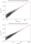 |
Fig. 21 Distribution of total hydrogen column densities in filaments. Top: NHtot as a function of length P/2. The fit ln(NHtot) = 47.0 ± 0.02 + (1.345 ± 0.008) ln(P/2) is indicated by the red line. Bottom: NHtot as a function of surface nS and with the fit ln(NHtot) = 47.1 ± 0.02 + (1.089 ± 0.005) ln(nS) shown as a red line. |
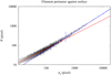 |
Fig. 22 Filament perimeters P as a function of surface counts nS. The fits ln(P) = 0.716 ± 0.007 + (0.749 ± 0.002)ln(nS) for nS < 500 (red) and ln(P) = −0.30 ± 0.08 + (0.94 ± 0.01)ln(nS) for nS > 500 (blue) are indicated, which correspond to fractal dimensions D = 1.5 and D = 1.9, respectively. |
4 Estimating the turbulent magnetic field strength
The magnetization of the ISM can be estimated by assuming that the energy of magnetic field fluctuations is in equipartition with the kinetic energy of turbulence (Alfvén 1949),
 (10)
(10)
where δB is the strength of the fluctuating part of the magnetic field and ρ is the volume density of the gas phase that is supplying the kinetic energy. Here, we need to consider the total amount of gas, including hydrogen and helium. We use the estimates of the molecular hydrogen content of H I clouds according to Kalberla et al. (2020; see also Sect. 3.7) and include a 34% correction for the helium mass fraction (Steigman 2007). It is assumed that the true velocity perturbations are isotropic, and therefore the dispersion in the velocity transverse to the filament spines is equal to the rms line-of-sight (LOS) velocity (Chandrasekhar & Fermi 1953) and ∆υLSR is the observed 1D LOS velocity dispersion along the filaments. Below, we discuss two cases, assuming filaments at a constant average distance and alternatively assuming the filaments to be located at the LB rim with distances as determined by Pelgrims et al. (2020).
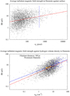 |
Fig. 23 Average turbulent magnetic field strength δB in filaments. Top: δB depending on filament surface ns. The fit ln(δB) = 0.46 ± 0.07 + (0.28 ± 0.02)ln(ns) is indicated by the red line. Bottom: average turbulent magnetic field strength in filaments δB as a function of the average hydrogen volume density. The fit ln(δB) = 0.66 ± 0.02 + (0.57 ± 0.01) ln(nH) for all 6568 filaments is indicated in red. Fitting only prominent filaments with surfaces for ns > 500 (right from the vertical blue line in the top figure), we get ln(δB) = 1.0 ± 0.1 + (0.52 ± 0.04)ln(nH), as indicated by the blue line. The orange arrow points from the center of mass of the point cloud (〈nH〉 = 8.0 cm−3, 〈δB〉 = 7.9 μG) -assuming a distance of 100 pc – to the center of mass (〈nH〉 = 3.2 cm−3, 〈δB〉 = 5.0 μG) for a distance of 250 pc. |
4.1 Distance dependencies
A generally accepted model assumption is that winds and supernova explosions inflated the LB of gas and dust. The cavity wall was stretched to create the aligned filaments and magnetic field lines that we observe. For many years, the distance to the LB wall remained unknown and it became common to use 100 pc as a fiducial number (Sfeir et al. 1999). Below we describe how we followed this assumption first in order to derive results that are comparable to previously published findings, and then explored how the results change with distance.
Using the parameters from the previous section, we derived an average magnetic field strength of 〈δB〉 = 7.9 μG for an average distance of 100 pc. The distribution of δB for all filaments is shown in Fig. 23. The top panel displays δB as a function of surface ns. As expected from previous discussions, filaments with large surfaces tend to be associated with higher magnetic fields; the correlation coefficient here is 0.28. For ns > 500, we find the average 〈δB〉 = 14.2 μG. The lower plot in Fig. 23 displays B as a function of nH. We find a general trend of  , which is indicated with the red line. The blue line shows a similar trend for prominent filaments with ns > 500.
According to recent distance determinations, which are discussed in the following subsection in more detail, most of the LB wall is located at distances of between 200 and 300 pc (Pelgrims et al. 2020). To estimate distance biases, we considered dependencies on our estimates for the averages of 〈nH〉 = 8.0 cm−3, 〈δB〉 = 7.9 μG, at a distance of 100 pc, by changing the assumed distance to 250 pc. We obtain 〈nH〉 = 3.2 cm−3, 〈δB〉 = 5.0 μG. The resulting average bias is indicated in Fig. 23 with an orange arrow. For filamentary structures with variable distances, we expect that the distribution shown in this figure can be stretched by shifting individual data points up to the amount indicated by the orange arrow.
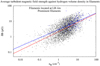 |
Fig. 24 Average turbulent magnetic field strength in filaments δB as a function of the average hydrogen volume density for filaments located at the LB wall. The fit ln(δB) = 0.71 ± 0.02 + (0.59 ± 0.01) ln(nH) for all 6568 filaments is indicated in red. When fitting only prominent filaments with surfaces for ns > 500 (right from the vertical blue line in Fig. 23 top), we get ln(δB) = 1.03 ± 0.09 + (0.53 ± 0.04)ln(nH) as indicated by the blue line. |
4.2 Filaments at the rim of the Local Bubble
Figure 24 shows the distribution of the turbulent magnetic field strength δB using recent distance estimates. Pelgrims et al. (2020) determined the geometry of the LB shell from 3D dust extinction maps. We use distances for the inner surface of the LB shell as extracted from the Lallement et al. (2019) extinction map shown in the top panel of Fig. 4 in Pelgrims et al. (2020). The spread in distance is 81 < D < 366 pc. We verified that distances within the filaments are homogeneous, and find no significant scatter in distance within individual filaments. Furthermore, we find no distance dependencies for filament width or velocity.
As expected, Fig. 24 shows a somewhat stretched data distribution. We derive  on average and
  for prominent filaments. The average turbulent magnetic field strength is 〈δB〉 = 5.3 μG at an average filament volume density of 〈nH〉 = 3.8 cm−3. In the case of prominent filaments, we obtain 〈δB〉 = 9.5 μG and 〈nH〉 = 8.6 cm−3. The average magnetic field strength is only 6% higher than the estimates in Sect. 4.1 in the case of a constant distance of 250 pc. Our exercise in Sect. 4.1 demonstrates that regional distance uncertainties cannot affect the average turbulent magnetic field strength significantly. We repeated our analysis, this time also using the model extinction map with a spherical harmonic expansion up to lmax = 6, shown at the bottom of Fig. 4 in Pelgrims et al. (2020). We find changes in the scatter diagram but no significant changes in the derived averages.
All filaments considered here have nH < 100 cm−3. Crutcher et al. (2010) and Crutcher (2012) note that in the range nH < 300 cm−3, which is characteristic for the diffuse ISM, δB does not scale with density. These authors conclude that diffuse clouds are assembled by flows along magnetic field lines, which would increase the density but not the magnetic field strength. Our case is different; we explicitly study filamentary structures driven by a turbulent small-scale dynamo. These structures are in direct interaction with turbulence-induced magnetic fields. Therefore, we consider a selective sample, occupying only 25% of the diffuse ISM. Pelgrims et al. (2020) modeled the magnetic field by fitting the Planck 353 GHz dust-polarized emission maps over the Galactic polar caps and concluded that the magnetic field in each polar cap is almost aligned with the plane of the sky. This result supports the validity of our approach, inserting the observed velocity dispersion in Eq. (10) without a correction for projection effects. We implicitly assume that the magnetic field is aligned with the plane of the sky. Our results do not necessarily contradict those of Crutcher et al. (2010), who consider Zeeman observations, where the magnetic field is along the line of sight, while Eq. (10) is valid for estimates of the field projected to the plane of the sky. Zeeman measurements suffer from sensitivity limitations, while estimates based on Eq. (10) are dominated by uncertainties in distance and volume density. The derived scaling with the magnetic field strength is in our case SB  , which is consistent with the MHD simulations of Seta & Federrath (2022) for the fluctuation dynamo in a compressible multiphase medium. These authors consider a compression of the magnetic field perpendicular to the magnetic field lines for the warm neutral medium (WNM), and therefore
  for cylindrical or filamentary geometry, and with their simulations obtain
  . A similar power-law scaling was obtained by Ponnada et al. (2022) from their simulations of filamentary cloud structures.
Studying the nature and the properties of the cold structures formed via thermal instability in the magnetized atomic ISM, Gazol & Villagran (2018, 2021) searched for clumps formed in forced MHD simulations with an initial magnetic field ranging from 0 to 8.3 μG. These authors find that a positive correlation between B and nH develops for all initial magnetic field intensities. The density at which this correlation becomes significant (nH ≲ 30 cm−3) depends on the initial conditions but is not sensitive to the presence of self-gravity. Figure 2 of Gazol & Villagran (2021) shows that the resulting clumps have a wide range of magnetic field intensities, which is similar to the large scatter that we observe here. The magnetic field in the simulations, albeit weak, qualitatively affects the morphology by producing filamentary structures.
5 Estimating the mean magnetic field strength
After considering estimates of the fluctuating magnetic field strength SB, we intend to discuss estimates of the mean magnetic field strength BPOS in the plane of the sky. For this parameter, we use four different estimates.
5.1 DCF-based methods
Davis (1951) and Chandrasekhar & Fermi (1953; DCF) introduced the basic approach to determining BPOS, which is usually formulated as
 (11)
(11)
Here, it is assumed that the velocity fluctuations are perpendicular to the magnetic field, and therefore ∆υLSR is the 1D line-of-sight dispersion in velocity (from turbulence, unaffected by thermal broadening). ∆θ is the dispersion of the orientation angles in the plane of the sky, reflecting transverse fluctuations of the magnetic field, and ξ is a correction factor, usually approximated as ξ ~ 0.5, that takes various physical and observational conditions (density inhomogeneities, anisotropies on velocity perturbations, observational resolution, and averaging effects) into account, (e.g., Zweibel 1990; Ostriker et al. 2001; Heitsch et al. 2001, Padoan et al. 2001 or Falceta-Gonçalves et al. 2008). The original DCF approach was ξ = 1. In the case where ∆θ ≲ 25°, a corrected factor ξ = 0.5 was determined by Ostriker et al. (2001) from MHD simulations. However, various authors noticed that this factor may be rather uncertain. Several attempts have been made to improve Eq. (11) and we discuss three cases for comparison.
Heitsch et al. (2001) proposed the modification
![Mathematical equation: ${B_{\rm{H}}} = \sqrt {4\pi \rho } {{{\rm{\Delta }}{\upsilon _{{\rm{LSR}}}}} \over {{\rm{\Delta }}\left( {\tan \theta } \right)}}{\left[ {1 + 3{\rm{\Delta }}{{\left( {\tan \theta } \right)}^2}} \right]^{{1 \mathord{\left/ {\vphantom {1 4}} \right. \kern-\nulldelimiterspace} 4}}}, $](/articles/aa/full_html/2023/05/aa45200-22/aa45200-22-eq35.png) (12)
(12)
and verified this approach with numerical simulations. These authors concluded that their modified version yields magnetic field estimates in molecular clouds accurate up to a factor of 2.5 even for the weakest fields.
Next, Falceta-Gonçalves et al. (2008) proposed the modification
 (13)
(13)
These authors noticed that, in some cases, BH tends to systematically underestimate the magnetic field intensity. They claim that their generalized equation for the DCF method allows them to determine the magnetic field strength from polarization maps with errors <20%.
The most recent reinvestigation of the DCF method was by Skalidis & Tassis (2021). These authors argue that the DCF method is based on the assumption that isotropic turbulent motions initiate the propagation of Alfvén waves. Skalidis & Tassis (2021) also consider non-Alfvénic (compressible) modes that have been proven to be important from observations but have not been considered in the DCF approach and modifications. Skalidis & Tassis (2021) derive the relation
 (14)
(14)
Extensive numerical tests of this method were carried out by Skalidis et al. (2021), who found that relaxing the incompress-ibility assumption leads to far more reliable magnetic field determinations for a broad range of parameters.
We use our data to determine the mean magnetic field strengths in the plane of the sky and compare the four different approaches mentioned above. Our approach is motivated by Pelgrims et al. (2020), who concluded from their best-fit model that, at high Galactic latitudes, the inclination of the mean magnetic field has only a small angle γ ~ 15° to the plane of the sky. Projection effects caused by such a misalignment should be negligible. We use the same distances to the LB rim as in Sect. 4.2. We determined the dispersion ∆θ of the orientation angles along individual filaments to be
![Mathematical equation: ${\rm{\Delta }}\theta = \,\,\,\sqrt {{1 \over {\sum\nolimits_{i = 1}^{{N_i}} {\,{N_j}\left( i \right)} }}\sum\limits_{i = 1}^{{N_i}} {{{\sum\limits_{j = 1}^{{N_j}\left( i \right)} {\,\left[ {\theta \left( {{{\bf{r}}_{\bf{i}}} + {\delta _j}} \right) - \theta \left( {{{\bf{r}}_{\bf{i}}}} \right)} \right]}^2 }}.} } $](/articles/aa/full_html/2023/05/aa45200-22/aa45200-22-eq38.png) (15)
(15)
This sum extends over all pixels ri along the filament with positions (ri·+ δj) within an annulus centered on r and with inner and outer radii of δ/2 and 3δ/2, respectively. According to the definition of the Hessian operator with adopted Gaussian smoothing over five pixels in Paper I, we select a lag of δ = 18'.
Figure 25 shows the derived distributions of BPOS as a function of nS for the four different estimates from Eqs. (11) to (14). Derived parameters for the ensemble averages 〈Bpos〉 and from fitting ln(BPOS) = a + b ln(nH) are listed in Table 1. Common to all four approaches is a scaling relation between magnetic field strength and volume density that is in conflict with the density-independent field strength determined by Crutcher et al. (2010). The ST results are similar to the results from Sect. 4.2 and we adopt  in the following. The most serious discrepancy in the derived scatter diagrams exists for Eq. (12), the H solution. This may be explained by the fact that Heitsch et al. (2001) put their focus on magnetized self-gravitating molecular clouds. The filaments that we discuss here certainly do not belong to this class. A significant discrepancy is also that these authors report that filaments produced in their MHD simulations by shocks do not show a preferred alignment with the magnetic field, which is incompatible with our sample.
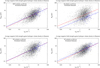 |
Fig. 25 Average plane of the sky magnetic field strength in filaments BPOS as a function of the average hydrogen volume density for filaments located at the LB wall. We distinguish DCF approaches Eq. (11) (top left) from those of Heitsch et al. (2001, H), Eq. (12) (top right), Falceta-Gonçalves et al. (2008, FG), Eq. (13) (bottom left), and Skalidis & Tassis (2021, ST), Eq. (14) (bottom right). Fit parameters are given in Table 1. |
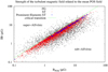 |
Fig. 26 Turbulent magnetic field strength δB as a function of the mean magnetic field component BPOS from Eq. ((13), FG, black dots) and Eq. ((14), ST, red dots). Overplotted in blue are prominent filaments with ns > 500 from Eq. ((14), ST). The green line indicates the critical transition for the magnetic field evolution according to Eq. (29) of Beattie etal. (2020). |
5.2 Relations between mean and turbulent magnetic fields
The distributions of BPOS in Fig. 25 show remarkable similarities to the distribution of the turbulent field from Fig. 24. We compare turbulent and mean field strengths in Fig. 26 for two cases, derived from Eqs. ((13), FG) and ((14), ST). Figure 26 tells us that turbulent and derived mean fields are correlated. We see the best correlation in the ST case (red) and in particular for prominent filaments (blue), with a correlation coefficient of 0.997. Derived parameters for prominent filaments are most significant because statistical errors are low in cases with a large number of surface elements ns. The scatter of the point cloud in the case of the FG solution is very large. Following the arguments of Skalidis & Tassis (2021) and Skalidis et al. (2021), there are systematic uncertainties in the DCF approach, as well as the H and FG derivatives, because compressible MHD wave modes have been ignored in these cases. Our results from Sect. 3.7 support the argument that compressibility is important. Significant column-density fluctuations indicate phase transitions; filaments indicate a highly compressible medium.
The approximate agreement between turbulent and mean magnetic field strengths may imply that the prominent filaments in particular tend to be critically affected by processes that regulate the energy balance between kinetic energy and magnetic field strength. Dependencies between the strength of turbulent and mean field were found in MHD simulations by Federrath (2016). Three regions with different properties for the growth of the turbulent magnetic field component were distinguished: the dynamo regime, and the intermediate and strong guide-field regimes. An approximate equilibrium between turbulent and mean magnetic fields was found at the transition between weak and strong guide fields, separating super- and sub-Alfvénic regimes; see Fig 8 of Federrath (2016). As shown by Beattie et al. (2020) in their Fig. 7, the critical Alfvénic Mach number where the turbulent magnetic field gets damped by the mean field is in the range 1 ≲ MA ≲ 2. Using relation (29) of these latter authors to derive a more specific limit for the transition between dominant turbulent kinetic energy and dominant large-scale magnetic field energy, we obtain \δB\/\BPOS\ = 1.7. This condition, identified by Beattie et al. (2020) as the critical transition for the magnetic field evolution, is indicated in Fig. 26 with a green line. This limit fits surprisingly well to the sharp boundary in Fig. 26 in the case of the ST solution (red). Velocity fluctuations interact with the magnetic field, causing a fluctuating magnetic field component. The interplay between strong magnetic fields (sub-Alfvénic) and supersonic velocity fluctuations (super-Alfvénic range) appears to be strongly affected at the critical transition. The fluctuating magnetic field component is clearly strongly limited. This limit, which can be explained with compressible magnetohydrodynamic turbulence models, is only observable in the ST solution, Eq. (14), but does not exist in the case of incompressible DCF models.
According to relation (29) of Beattie et al. (2020), the critical transition occurs in MHD simulations at an Alfvénic Mach number of MAcrit = l·44; see also Fig. 7 of Beattie et al. (2022). In the following, we intend to also compare this model prediction with observational data.
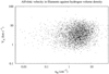 |
Fig. 27 Distribution of the Alfvén velocity υA according to Skalidis & Tassis (2021) as a function of the average hydrogen volume density nH for filaments. |
5.3 Alfvénic Mach numbers
To test the self-consistency of our ST solution, we first calculated the Alfvén velocities that have implicitly been used with Eq. (14); see Eq. (29) of Skalidis & Tassis (2021):
 (16)
(16)
The results are plotted in Fig. 27. This scatter diagram covers a large range in volume densities nh· This certainly reflects statistical uncertainties in the hydrogen column density estimates by Kalberla et al. (2020) to some extent, but υA is else unaffected by density effects. We also find no observable dependency of υA with respect to the filament surfaces. The mean Alfvén velocity is 4.7 km s−1, which is slightly less than the mean turbulent velocity dispersion of 5.24 km s−1.
Next, we calculate the Alfvénic Mach numbers. For individual filaments, according to Eq. (7) of Skalidis et al. (2021), we have
 (17)
(17)
and Fig. 28 shows the MAST distribution. There is no evidence that Alfvénic Mach numbers depend significantly on hydrogen volume densities. Furthermore, the range covered by the MAST distribution is consistent with the range MA < 2, which was tested by Skalidis et al. (2021) for the validity and reliability of the ST approach.
We derive a mean Alfvénic Mach number of 〈MAST〉 = 1.23 for all filaments. The prominent filaments with ns > 500 have 〈Mast〉 = 1.34. This is close to the critical Alfvénic Mach number MAcrit = 1 -44 from relation (29) of Beattie et al. (2020). Consistent with Fig. 26, we observe an upper limit of MAST < 1.7. Figure 28 implies a well-developed trans-Alfvénic turbulence for most of the filaments. This is the regime of MHD turbulence where anisotropic structures are expected in the case of an incompressible medium (Goldreich & Sridhar 1995). It is also the critical transition region where Federrath (2016) and Beattie et al. (2020, 2022) found energy equipartition between the turbulent and large-scale magnetic field in the case of compressible turbulence.
The observed sonic Mach numbers in filaments are typically MS ~ 3.7 (Heiles & Troland 2005 and Kalberla et al. 2016). Our results for prominent filaments shown in Fig. 26 are consistent with MHD simulations in a similar range, that is, MS ~ 3.5 with MA ~ 1.7 by Beattie et al. (2020), see their Table 1. In the case of supersonic turbulent flows, shocks are expected with phase transitions, which explains the observed exceptionally cold H I (Paper I, Sect. 3.1) and the large  excess that we discuss in Sect. 3.7. Filament motions excited by turbulence are affected by the magnetic field, but in the observed trans-Alfvénic range, turbulent velocity fluctuations along the filaments appear to remain confined such that the observed velocity coherence is usually preserved.
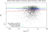 |
Fig. 28 Alfvénic Mach number in filaments as a function of the average hydrogen volume density for filaments located at the LB wall according to Eq. (17) based on Skalidis & Tassis (2021). The fit ln(MAST) = 0.179 ± 0.004 + (0.010 ± 0.003) ln(nH) for all 6568 filaments is indicated in red. Fitting only ns > 500 (right from the vertical blue line in Fig. 23 top), we get ln(MAST) = 0.30 ± 0.01 + (–0.005 ± 0.005) ln(nH), as indicated by the blue line. The green line indicates the critical transition for the magnetic field evolution according to Eq. (29) of Beattie et al. (2020). |
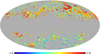 |
Fig. 29 Spatial distribution of the derived average magnetic-field strengths of filaments 〈BST〉 in Mollweide projection. The color coding is logarithmic for a range 0.1 < 〈BST〉 < 32μG. |
5.4 Results from the ST solution
Summarizing our results from the previous subsections, we derive a mean magnetic field strength for the ensemble average that is consistent with previous determinations (e.g., Heiles & Troland 2005 or Ferrière 2015). The conventional DCF approach and the modifications proposed by Heitsch et al. (2001) and Falceta-Gonçalves et al. (2008) show a larger intrinsic scatter than the ST solution (Skalidis et al. 2021).
We adopt the ST solution. Our ensemble averages of 〈BST〉 = 4.4 μG and 〈BST〉 = 7.1 μG for prominent filaments are consistent with the field strength of B0 = 6 + 1.8 μG derived by Heiles & Troland (2005). For turbulent as well as for mean magnetic field strengths, we find an average scaling relation of  . We confirm the models by Federrath (2016) and Beattie et al. (2020, 2022) with the prediction of a critical transition for the magnetic-field evolution that imposes upper limits on the strengths of mean-field normalized magnetic field fluctuations.
Figure 29 displays 〈BST〉 averaged over a pixel size of 27.5 and gridded to an nside = 128 HEALPix array. Large-scale structures are visible that resemble to some extent the large-scale magnetic-field distribution indicated by rotation measures shown in Fig. 3 of Oppermann et al. (2012), Fig. 7 of Sobey et al. (2019), or Fig. 1 of Dickey et al. (2022). The Faraday rotation of linearly polarized radiation at radio wavelengths is affected by the thermal electron density in the warm ionized medium and the line-of-sight component of the magnetic field (e.g., Oppermann et al. 2012, Eq. (1)). The FIR/H I filaments are embedded in this diffuse medium and it is plausible that turbulent and mean magnetic fields associated with filaments can be affected by the large-scale Galactic magnetic field. The average large-scale magnetic field strength in the Galactic halo is estimated to be ~4μG by Sobey et al. (2019, Table 3), which is consistent with our estimate.
5.5 Application to Loops I and IV
The radio sky at high Galactic latitudes is dominated by several bright spurs and loops in radio continuum that are interpreted as synchrotron radiation caused by supernova remnants (Berkhuijsen et al. 1971). In a recent analysis, Panopoulou et al. (2021) consider three tracers of the magnetic field: stellar polarization, polarized synchrotron radio emission, and polarized thermal dust emission. These authors use the alignment between these three tracers to constrain estimates of the distance to the synchrotron spurs. In a similar way, the alignment of filamentary FIR and H I structures was analyzed in Paper I; both publications followed the same basic assumption that an agreement in angular orientation must be indicative of a physical correlation. Distances obtained by Panopoulou et al. (2021) for fields with diameters of 16°are summarized in Table 2 together with our determination of the average field strengths 〈δB〉 and (BST) according to Eqs. (10) and (14) for filaments at such distances. In addition, we display BST for loops I and IV in Fig. 30. Except for a tendency toward higher volume densities, these results support our previous results and conclusions as to the H I counterparts of the synchrotron loops. These regions contain prominent FIR/H I filamentary structures (see Fig. 18 of Paper I) and have particularly well-aligned orientation angles between synchrotron emission and thermal dust. The H I filaments in loop I are dominated by a single spectral feature that accounts for 100% of the hydrogen column density (Das et al. 2020). Systematic errors are unexpected in this case.
The distance to loop I is a matter of debate. Sofue (2015) determined a distance of at least 1 kpc and Mou et al. (2022) estimated a magnetic field strength of 4 μG for this case. We determine accordingly 〈δB〉 = 2.2 μG and 〈BST〉 = 2.7 μG for loop Ib. This does not agree with the results listed in Table 2, nor with the results in the previous subsection.
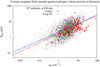 |
Fig. 30 Average plane-of-the-sky magnetic field strength in filaments, replicating the bottom right panel of Fig. 25 but annotating now BST derived for loops I (red) and IV (green) according to distances from Table 2. |
Locations and distances for the loop I and IV regions according to Panopoulou et al. (2021) with derived magnetic field strengths.
5.6 Uncertainties and biases
The estimates of the magnetic field strengths δB and BST in the previous subsections are based on the assumption of energy equipartition between magnetic field and kinetic energy (Alfvén 1949). Such an approach may be invalid for individual objects but should be justified on large scales or alternatively for averages over a large number of objects (Beck et al. 2003). In our case, we have 6568 filaments with significant individual uncertainties. In the case of a random error distribution, uncertainties for the ensemble average are reduced by a factor of 80.
For a filamentary field geometry, the lateral component of the velocity is effective (Chandrasekhar & Fermi 1953). The investigations by Pelgrims et al. (2020) indicate that at high Galactic latitudes, the inclination of the mean magnetic field has only a small angle γ ~ 15° to the plane of the sky. Uncertainties from projection effects are at the level of 4%. Statistical uncertainties from individual volume density estimates are large but we expect that systematical biases for averages in case of prominent filaments are limited to the percentage level. Systematic errors from distance uncertainties can be estimated by comparing the results from Sects. 4.1 and 4.2 and are below 6%.
The question remains as to whether particular DCF-based methods might lead to systematic errors. Table 1 indicates that the derived BPOS can differ by a factor of up to four. Crutcher (2012) estimates that errors from the DCF approach can amount to a factor of two on average. Our investigations indicate that systematic differences are introduced in particular by compressibility issues. The ST solution of Eq. (14) is incompatible with the other DCF-based methods of Eqs. (11) to (13). Furthermore, only BPOS = BST from the ST solution shows an upper limit to |δB|/|BPOS| for the expected equilibrium between turbulent and mean magnetic fields as predicted by Federrath (2016) and Beattie et al. (2020, 2022). Our results strongly support compressible quasi-static fluctuation models (Fig. 26) but we cannot come to any conclusions about the level of systematic discrepancies between these models and alternative models that assume an incompressible medium based on the present study. Tests by Skalidis et al. (2021) demonstrated that the ST method of Eq. (14) has an accuracy of better than 50% for the range 0.1 ≲ MA ≲ 2.0. However, these authors admit that models with MA ≳ 0.7 tend to underestimate the magnetic field strength BST. This may affect our results, shown in Fig. 26, in the range close to |δB|/|BST| = 1.7 somewhat, but we did not apply any correction.
The typical strength of the random component of the local Galactic magnetic field is 5 ± 2 μG; the estimate for the local regular field amounts to 4 ± 1 μG, but Beck et al. (2003) caution that systematical errors of up to a factor of two are possible. Here, we notice that also these estimates are consistent with a critical balance between fluctuating and regular magnetic fields. Altogether, our total averages from Sects. 4.2 and the ST solution from 5.1 are compatible with these field strengths, and also with the value of B0 = 6 ± 1.8 μG derived by Heiles & Troland (2005).
We derived the field strengths for four fields with H I counterparts of the synchrotron loops I and IV. These regions contain prominent FIR/H I filamentary structures and have particularly well-aligned orientation angles between synchrotron emission and thermal dust. The H I filaments in loop I are dominated by a single spectral feature that accounts for 100% of the hydrogen column density (Das et al. 2020). Significant systematic errors from observations and data reduction are expected to be low in this case; the derived field estimates should at least be internally consistent.
6 Discussion
Our analysis is based on a Hessian analysis in Paper I and here we discuss our results. FIR filaments that are considered to be dusty magnetized structures are associated with H I filaments in narrow velocity intervals with a well-defined coherent velocity field along the filaments. Orientation angles of the FIR at 857 GHz are closely related to H I orientation angles that define the filament velocities. The distribution of filament curvatures was found to match that expected from models for magnetic-field curvatures induced by a Galactic small-scale turbulent dynamo (Schekochihin et al. 2004). We conclude that these filaments must have been shaped by interactions between the turbulent velocity field and induced magnetic fields. We are refining the analysis from Paper I and trace individual FIR filaments along the plane of the sky. We also find well-defined and coherent velocities for individual filaments, with a typical dispersion of ∆υLSR = 5.24 km s−1. This value is comparable to characteristic turbulent motions ∆υLSR = 5.9 km s−1 within the warm neutral medium (Saury et al. 2014).
The common FIR/H I structures define a network of filaments and we determined aspect ratios and filamentarities for 6568 structures. We find that aspect ratios and filamentarities are closely related to each other. The observed distribution follows the 𝒜-to-ℱ relation (9) expected for thin filaments. Filamentary networks are self-replicating, and the merger or disruption of structures means a repositioning of individual fragments on the 𝒜-to-ℱ track, but the general relation (9) shown in the top panel of Fig. 9 remains satisfied. Projection effects alter the observed aspect ratios but do not lead to deviations from this relation. We conclude that the observed continuous 𝒜-to-ℱ distribution cannot be significantly affected by observational artifacts or projection effects. Aspect ratios are measured as ratios between length and widths and are therefore independent of distance. However, from our independent width measurements, we find some indications that filaments with 𝒜 ≳ 100 tend to be associated with larger widths. These filaments may be at shorter distances but Fig. 7 shows an increase in W with increasing eigenvalue–λ_, implying stronger FIR/H I ridges. Results in Paper I suggest that stronger ridges are associated with stronger magnetic fields and lower curvatures, as predicted by Schekochihin et al. (2004). In Sect. 4, we find that the magnetic field is stronger in filaments with larger surfaces. Comparing filament widths with distances to the LB wall, we find no indications for a distance dependency.
Overall, we conclude that the observed FIR/H I filaments populate a well-defined continuous distribution in 𝒜 and ℱ with aspect ratios of up to a few hundred. In our analysis, we meet only two limitations. 𝒜 and ℱ are ill defined for surface counts nS < 10. Also, large structures with nS > 20 000 pixels cannot be analyzed because of confusion. This does not imply that filamentary structures with large aspect ratios cannot exist. The famous dust filament shown in Fig. 17 with 𝒜 ≳ 787 is a prominent example, but was excluded from our analysis because of the exceedingly large total surface of the filament.
In Paper I, we present evidence that FIR filaments are associated with exceptionally cold H I. Such H I clouds are expected to host molecular gas and in turn this H2 component is also expected to be filamentary. We use the CO-dark H2 distribution derived by Kalberla et al. (2020) by adopting the hypothesis of a constant E(B – V)/NH ratio and determine how the molecular gas content depends on aspect ratio. We find a significant increase in the molecular gas content with 𝒜. Comparing NH column densities within filaments with that outside of them, the excess is  . For positions in the filament centers, this increases to a factor of 1.56. Accounting for CO-dark H2 only, we obtain an average column density excess of 4.32 along the filaments and 5.29 for the filament centers. Accounting only for prominent filaments with ns > 500, we get another enhancement by ~20%. In comparison to brightness temperature enhancements by a factor of 1.3 for filaments in the Herschel Gould Belt Survey (Koch & Rosolowsky 2015), column density fluctuations for filaments in the diffuse ISM are very strong. We conclude that the filaments discussed here are part of a homogeneous population of structures with strong density enhancements in gas and dust.
7 Summary and conclusions
Assuming that the energy of the magnetic field is in equipartition with the kinetic energy of turbulence (e.g. Groves et al. 2003), we derive an average scaling relation of  for both the fluctuating and mean magnetic field. We determine an average filament volume density of nH ~ 3.8 cm−3 with a turbulent field strength of 〈δB〉 = 5.3 μG and a mean field of 〈BST〉 = 4.4 μG, which are good agreement with the canonical field strength of B0 = 6 ± 1.8 μG derived by Heiles & Troland (2005) from H I data. Other observations that support B0 ~ 5 μG were discussed by Ferrière (2015).
We used a Hessian analysis to determine filamentary structures in the FIR and repeated this as a multi-channel analysis in H I to determine velocities and derived properties of the filaments. A complete morphological description of diffuse FIR/H I structures demands a full 3D analysis which is not available from observations. However, from simulations, it is possible to consider shape finders for pancakes, ribbons, and filaments (e.g., Sahni et al. 1998). MHD simulations of the fluctuation dynamo with morphological analyses in 3D by Wilkin et al. (2007) indicate that – at least at the kinematic stage – the magnetic field is concentrated into filaments rather than sheets or ribbons. Seta et al. (2020) find that the magnetic-field correlation length scale increases as the field saturates. The increase in the length of magnetic structures with saturation is consistent with the finding by Schekochihin et al. (2004) that a linear velocity field (as observed by us) allows the field to reach large aspect ratios between folds. Wilkin et al. (2007) and Seta et al. (2020) use for their morphological analysis isosurfaces at a fixed value of the magnetic field strength. This implies a preference for structures of stronger fields with less curvature (Schekochihin et al. 2004). As shown by Seta et al. (2020), the magnetic correlation scale in the saturated state moves to larger scales. The length scales associated with both the greatest stretching and compression grow as the magnetic field saturates (Seta & Federrath 2021). These results are consistent with the large aspect ratios that we observed. Complex filamentary shapes in 3D may be responsible for the filamentary network, as observed here in projection.
Concerning the 3D structure of the ISM, the existence of a correlation between local H I volume density enhancements as real physical objects and magnetic field structures was questioned by Lazarian & Yuen (2018) and Yuen et al. (2021). According to Lazarian & Pogosyan (2000), a gaseous incompressible fluid in turbulent motion, even when uniformly distributed in space, produces the fluctuating emission structures when observed in a velocity slice of finite thickness. Clark et al. (2019) were the first to demonstrate that this hypothesis is not verified by data. Furthermore, we showed in Paper I that velocity coherence along the filaments cannot be generated by random processes.
We interpret our H I structures as filaments in a compressible medium, and therefore as real physical entities. Such structures, which are observable in projection with strong column density enhancements, cannot be generated by random events that accumulate unrelated H I along the line of sight. We confirm the findings from compressible magnetohydrodynamic turbulence models by Federrath (2016) and Beattie et al. (2020, 2022) in particular their prediction of a critical transition for the magnetic field evolution with upper limits for the strength of mean-field normalized magnetic field fluctuations.
Acknowledgements
We appreciate valuable comments and suggestions from the referee, which helped us in improving the quality of the manuscript. P.K. acknowledges discussions with Susan Clark, Jürgen Kerp, Vincent Pelgrims, and Rafail Skalidis. In particular the discussions with Amit Seta were very helpful. HI4PI is based on observations with the 100-m telescope of the MPIfR (Max-Planck- Institut für Radioastronomie) at Effelsberg and the Parkes Radio Telescope, which is part of the Australia Telescope and is funded by the Commonwealth of Australia for operation as a National Facility managed by CSIRO. This research has made use of NASA’s Astrophysics Data System. Some of the results in this paper have been derived using the HEALPix package.
References
- Alfvén, H. 1949, Phys. Rev., 75, 1732 [Google Scholar]
- Beattie, J. R., Federrath, C., & Seta, A. 2020, MNRAS, 498, 1593 [Google Scholar]
- Beattie, J. R., Krumholz, M. R., Skalidis, R., et al. 2022, MNRAS, 515, 5267 [NASA ADS] [CrossRef] [Google Scholar]
- Beck, R., Shukurov, A., Sokoloff, D., et al. 2003, A&A, 411, 99 [NASA ADS] [CrossRef] [EDP Sciences] [Google Scholar]
- Berkhuijsen, E. M., Haslam, C. G. T., & Salter, C. J. 1971, A&A, 14, 252 [NASA ADS] [Google Scholar]
- Bharadwaj, S., Sahni, V., Sathyaprakash, B. S., et al. 2000, ApJ, 528, 21 [NASA ADS] [CrossRef] [Google Scholar]
- Chandrasekhar, S., & Fermi, E. 1953, ApJ, 118, 113 [Google Scholar]
- Clark, S. E., Peek, J. E. G., & Putman, M. E. 2014, ApJ, 789, 82 [NASA ADS] [CrossRef] [Google Scholar]
- Clark, S. E., Peek, J. E. G., & Miville-Deschênes, M.-A. 2019, ApJ, 874, 171 [NASA ADS] [CrossRef] [Google Scholar]
- Criscuoli, S., Rast, M. P., Ermolli, I., et al. 2007, A&A, 461, 331 [NASA ADS] [CrossRef] [EDP Sciences] [Google Scholar]
- Crutcher, R. M. 2012, ARA&A, 50, 29 [Google Scholar]
- Crutcher, R. M., Wandelt, B., Heiles, C., et al. 2010, ApJ, 725, 466 [NASA ADS] [CrossRef] [Google Scholar]
- Das, K. K., Zucker, C., Speagle, J. S., et al. 2020, MNRAS, 498, 5863 [Google Scholar]
- Davis, L. 1951, Phys. Rev., 81, 890 [Google Scholar]
- Dickey, J. M., West, J., Thomson, A. J. M., et al. 2022, ApJ, 940, 75 [NASA ADS] [CrossRef] [Google Scholar]
- Falceta-Gonçalves, D., Lazarian, A., & Kowal, G. 2008, ApJ, 679, 537 [Google Scholar]
- Falgarone, E., Phillips, T. G., & Walker, C. K. 1991, ApJ, 378, 186 [NASA ADS] [CrossRef] [Google Scholar]
- Federrath, C. 2016, J. Plasma Phys., 82, 535820601 [Google Scholar]
- Ferrière, K. 2015, J. Phys. Conf. Ser., 577, 012008 [CrossRef] [Google Scholar]
- Gazol, A., & Villagran, M. A. 2018, MNRAS, 478, 146 [CrossRef] [Google Scholar]
- Gazol, A., & Villagran, M. A. 2021, MNRAS, 501, 3099 [NASA ADS] [CrossRef] [Google Scholar]
- Goldreich, P., & Sridhar, S. 1995, ApJ, 438, 763 [Google Scholar]
- Górski, K. M., Hivon, E., Banday, A. J., et al. 2005, ApJ, 622, 759 [Google Scholar]
- Groves, B. A., Cho, J., Dopita, M., et al. 2003, PASA, 20, 252 [NASA ADS] [CrossRef] [Google Scholar]
- Hacar, A., Clark, S., Heitsch, F., et al. 2022, ArXiv e-prints [arXiv:2203.09562] [Google Scholar]
- Heiles, C., & Troland, T. H. 2005, ApJ, 624, 773 [NASA ADS] [CrossRef] [Google Scholar]
- Heitsch, F., Zweibel, E. G., Mac Low, M.-M., et al. 2001, ApJ, 561, 800 [NASA ADS] [CrossRef] [Google Scholar]
- Hennebelle, P., & Inutsuka, S.-S.-I. 2019, Front. Astron. Space Sci., 6, 5 [NASA ADS] [CrossRef] [Google Scholar]
- HI4PI Collaboration (Ben Bekhti, N., et al.) 2016, A&A, 594, A116 [NASA ADS] [CrossRef] [EDP Sciences] [Google Scholar]
- Kalberla, P. M. W., & Haud, U. 2015, A&A, 578, A78 [NASA ADS] [CrossRef] [EDP Sciences] [Google Scholar]
- Kalberla, P. M. W., Kerp, J., Haud, U., et al. 2016, ApJ, 821, 117 [Google Scholar]
- Kalberla, P. M. W., Kerp, J., & Haud, U. 2020, A&A, 639, A26 [EDP Sciences] [Google Scholar]
- Kalberla, P. M. W., Kerp, J., & Haud, U. 2021, A&A, 654, A91 [NASA ADS] [CrossRef] [EDP Sciences] [Google Scholar]
- Kerscher, M. 2000, Statistical Physics and Spatial Statistics. The Art of Analyzing and Modeling Spatial Structures and Pattern Formation (Berlin: Springer), 36 [Google Scholar]
- Koch, E. W., & Rosolowsky, E. W. 2015, MNRAS, 452, 3435 [Google Scholar]
- Lallement, R., Babusiaux, C., Vergely, J. L., et al. 2019, A&A, 625, A135 [NASA ADS] [CrossRef] [EDP Sciences] [Google Scholar]
- Lazarian, A., & Pogosyan, D. 2000, ApJ, 537, 720 [NASA ADS] [CrossRef] [Google Scholar]
- Lazarian, A., & Yuen, K. H. 2018, ApJ, 853, 96 [NASA ADS] [CrossRef] [Google Scholar]
- Legland, D., Kiêu, & Devaux, M.-F., Image Anal. Stereol., 2, 83. [Google Scholar]
- Lehmann, G., & Legland, D., 2012, https://doi.org/10.54294/wdu86d [Google Scholar]
- Makarenko, I., Fletcher, A., & Shukurov, A. 2015, MNRAS, 447, L55 [NASA ADS] [CrossRef] [Google Scholar]
- Mandelbrot, B. B. 1982, The fractal geometry of nature (New York, W.H. Freeman and Co.), 495 [Google Scholar]
- Mandelbrot, B. B., Passoja, D. E., & Paullay, A. J. 1984, Nature, 308, 721 [NASA ADS] [CrossRef] [Google Scholar]
- Mecke, K. R., & Stoyan, D. 2000, Statistical Physics and Spatial Statistics: The Art of Analyzing and Modeling Spatial Structures and Pattern Formation, (Springer-Verlag Berlin and Heidelberg GmbH & Co) 554 [Google Scholar]
- Mecke, K. R., Buchert, T., & Wagner, H. 1994, A&A, 288, 697 [NASA ADS] [Google Scholar]
- Meunier, N. 1999, ApJ, 515, 801 [NASA ADS] [CrossRef] [Google Scholar]
- Mou, G., Wu, J., & Sofue, Y. 2022, A&A submitted, [arXiv:2212.04306] [Google Scholar]
- Oppermann, N., Junklewitz, H., Robbers, G., et al. 2012, A&A, 542, A93 [NASA ADS] [CrossRef] [EDP Sciences] [Google Scholar]
- Ostriker, E. C., Stone, J. M., & Gammie, C. F. 2001, ApJ, 546, 980 [Google Scholar]
- Padoan, P., Goodman, A., Draine, B. T., et al. 2001, ApJ, 559, 1005 [Google Scholar]
- Panopoulou, G. V., Dickinson, C., Readhead, A. C. S., et al. 2021, ApJ, 922, 210 [CrossRef] [Google Scholar]
- Peek, J. E. G., Babler, B. L., Zheng, Y., et al. 2018, ApJS, 234, 2 [Google Scholar]
- Pelgrims, V., Ferrière, K., Boulanger, F., et al. 2020, A&A, 636, A17 [NASA ADS] [CrossRef] [EDP Sciences] [Google Scholar]
- Planck Collaboration Int. XXXII. 2016, A&A, 586, A135 [NASA ADS] [CrossRef] [EDP Sciences] [Google Scholar]
- Planck Collaboration Int. LVII. 2020, A&A, 643, A42 [NASA ADS] [CrossRef] [EDP Sciences] [Google Scholar]
- Ponnada, S. B., Panopoulou, G. V., Butsky, I. S., et al. 2022, MNRAS, 516, 4417 [NASA ADS] [CrossRef] [Google Scholar]
- Sahni, V., Sathyaprakash, B. S., & Shandarin, S. F. 1998, ApJ, 495, L5 [NASA ADS] [CrossRef] [Google Scholar]
- Saury, E., Miville-Deschênes, M.-A., Hennebelle, P., et al. 2014, A&A, 567, A16 [NASA ADS] [CrossRef] [EDP Sciences] [Google Scholar]
- Schekochihin, A. A., Cowley, S. C., Taylor, S. F., et al. 2004, ApJ, 612, 276 [NASA ADS] [CrossRef] [Google Scholar]
- Seta, A., & Federrath, C. 2021, Phys. Rev. Fluids, 6, 103701 [NASA ADS] [CrossRef] [Google Scholar]
- Seta, A., & Federrath, C. 2022, MNRAS, 514, 957 [NASA ADS] [CrossRef] [Google Scholar]
- Seta, A., Bushby, P. J., Shukurov, A., et al. 2020, Phys. Rev. Fluids, 5, 043702 [NASA ADS] [CrossRef] [Google Scholar]
- Sfeir, D. M., Lallement, R., Crifo, F., et al. 1999, A&A, 346, 785 [NASA ADS] [Google Scholar]
- Skalidis, R., & Tassis, K. 2021, A&A, 647, A186 [NASA ADS] [CrossRef] [EDP Sciences] [Google Scholar]
- Skalidis, R., Sternberg, J., Beattie, J. R., et al. 2021, A&A, 656, A118 [NASA ADS] [CrossRef] [EDP Sciences] [Google Scholar]
- Sobey, C., Bilous, A. V., Grießmeier, J.-M., et al. 2019, MNRAS, 484, 3646 [NASA ADS] [CrossRef] [Google Scholar]
- Sofue, Y. 2015, MNRAS, 447, 3824 [NASA ADS] [CrossRef] [Google Scholar]
- Soler, J. D., Beuther, H., Syed, J., et al. 2020, A&A, 642, A163 [NASA ADS] [CrossRef] [EDP Sciences] [Google Scholar]
- Soler, J. D., Miville-Deschênes, M.-A., Molinari, S., et al. 2022, A&A, 662, A96 [NASA ADS] [CrossRef] [EDP Sciences] [Google Scholar]
- Stawiaski, J., Decencière, E., & Bidault, F. 2007 Proceedings of the 8 th International Symposium on Mathematical Morphology, MCT/INPE, v. 1, 349 [Google Scholar]
- Steigman, G. 2007, Ann. Rev. Nucl. Part. Sci., 57, 463 [Google Scholar]
- Wilkin, S. L., Barenghi, C. F., & Shukurov, A. 2007, Phys. Rev. Lett., 99, 134501 [NASA ADS] [CrossRef] [Google Scholar]
- Winkel, B., Kerp, J., Flöer, L., et al. 2016, A&A, 585, A41 [NASA ADS] [CrossRef] [EDP Sciences] [Google Scholar]
- Yuen, K. H., Ho, K. W., & Lazarian, A. 2021, ApJ, 910, 161 [NASA ADS] [CrossRef] [Google Scholar]
- Zweibel, E. G. 1990, ApJ, 362, 545 [Google Scholar]
HFI_SkyMap_857_2048_R4.00_full.fits and HFI_SkyMap_545_ 2048_R4.00_full.fits, and HFI_SkyMap_353-field-IQU_2048_R4.00_full.fits from https://irsa.ipac.caltech.edu/data/Planck/release_3/ancillary-data/HFI_Products.html
There are eight HEALPix positions on the sky with only seven neighbors.
Errors given throughout this paper are dispersions rounded to a significant digit. In this case, we derived ℱ/ℱmodel = 0.999974 ± 8.097 × 10⁻⁴ from 114 samples with variable widths with a different realization.
Throughout the paper, for fitting a set of data points, we use an implementation of the nonlinear least-squares Marquardt-Levenberg algorithm provided by Gnuplot and cite rounded formal asymptotic standard errors of the fit.
All Tables
Locations and distances for the loop I and IV regions according to Panopoulou et al. (2021) with derived magnetic field strengths.
All Figures
|
Fig. 1 Average filament widths derived from neighbor counts during simulations. |
| In the text | |
|
Fig. 2 Spatial distribution of filaments with width W as function of latitude b. |
| In the text | |
|
Fig. 3 Cumulative distribution function of velocity separations ΔυGauss = |υnear − υdominant| between Gaussian components associated with H I filaments that are nearest in velocity and dominant in column density. |
| In the text | |
|
Fig. 4 Distribution of the 6568 FIR/H I filaments in Mollweide projection. The horizontal lines indicate Galactic latitudes of b = 20° and b = −20°. |
| In the text | |
|
Fig. 5 Spatial distribution of filaments with width W for 10 < nS < 20 000, as a function of latitude b (top) and longitude l (bottom). |
| In the text | |
|
Fig. 6 Average filament width W as a function of filament surface, measured by counting surface pixels nS. The red line represents the fit W = 0.74 ± .01 + (0.491 ± .004)ln(nS) |
| In the text | |
|
Fig. 7 Average filament width W as a function of the average Hessian eigenvalue −λ− from 857 GHz data. |
| In the text | |
|
Fig. 8 Filamentarity of 6568 structures as a function of filament surface measured by counting filament surface pixels nS. The dashed blue line shows a model of the filamentarity in the case of a constant width of W = 2.53 pixels, and the red line shows the model for the broadening fit from Fig. 6. Formal numerical 3σ uncertainties from perimeter counts are indicated by the dash-dotted orange lines. |
| In the text | |
|
Fig. 9 Distribution of filaments covering the parameter space in aspect ratio 𝒜 and filamentarity ℱ. The distribution in the top panel was derived using the width W as described in Sect. 2.2.2 for each filament. For the distribution in the bottom panel, we use widths as determined from the fit described in Sect. 3.2. The dashed yellow line is derived from Eq. (9) using aspect ratios according to Eq. (7). Positions marked in red in the upper plot belong to the two filaments described in Sect. 3.6; merging these filaments results in a single structure, marked with blue. |
| In the text | |
|
Fig. 10 Probability density distributions of filamentarities ℱ. Top: distribution by number. Bottom: distribution weighted by the total surface covered by filaments. |
| In the text | |
|
Fig. 11 Probability density distributions of aspect ratios 𝒜. Top: distribution by number. Bottom: distribution weighted by the total surface covered by filaments. |
| In the text | |
|
Fig. 12 Velocity distribution as a function of aspect ratio. Top: average filament H I radial velocities. Bottom: velocity dispersions within the filaments. |
| In the text | |
|
Fig. 13 Fraction O of outlier positions depending on filament surface nS. Outliers are defined as positions with velocities deviating from the average filament velocity by more than three times the velocity dispersion. The presentation is strongly quantized, showing, from bottom to top, outlier counts of zero, one, two, and so on. The blue vertical line divides the sample at nS = 500. |
| In the text | |
|
Fig. 14 Fraction O of outlier positions as a function of the average Hessian eigenvalue −λ− from the FIR data. Blue data points are from prominent filaments with nS > 500. |
| In the text | |
|
Fig. 15 Spatial distribution of filamentary structures in gnomonic projection. The field size is 27°.7. Top: isolated filamentary structures discussed in the text. For each position, the color coding shows weights according to the number of neighbors nNeighbor inside the filament. Boundary pixels nPout just outside the filaments have weight −1 and are coded in blue. Bottom: velocity field of the filamentary structures, including all other filaments in the field. The center position is l = 260°, b = 58°. |
| In the text | |
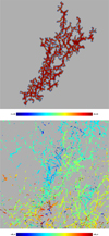 |
Fig. 16 As in Fig. 15 but centered at l = 45°, b = 42°. |
| In the text | |
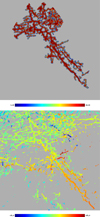 |
Fig. 17 As in Fig. 15 but centered at l = 283°, b = −43°. |
| In the text | |
|
Fig. 18 Excess in total hydrogen column density |
| In the text | |
|
Fig. 19 Excess in total hydrogen column density |
| In the text | |
|
Fig. 20 Excess in total hydrogen column density |
| In the text | |
|
Fig. 21 Distribution of total hydrogen column densities in filaments. Top: NHtot as a function of length P/2. The fit ln(NHtot) = 47.0 ± 0.02 + (1.345 ± 0.008) ln(P/2) is indicated by the red line. Bottom: NHtot as a function of surface nS and with the fit ln(NHtot) = 47.1 ± 0.02 + (1.089 ± 0.005) ln(nS) shown as a red line. |
| In the text | |
|
Fig. 22 Filament perimeters P as a function of surface counts nS. The fits ln(P) = 0.716 ± 0.007 + (0.749 ± 0.002)ln(nS) for nS < 500 (red) and ln(P) = −0.30 ± 0.08 + (0.94 ± 0.01)ln(nS) for nS > 500 (blue) are indicated, which correspond to fractal dimensions D = 1.5 and D = 1.9, respectively. |
| In the text | |
|
Fig. 23 Average turbulent magnetic field strength δB in filaments. Top: δB depending on filament surface ns. The fit ln(δB) = 0.46 ± 0.07 + (0.28 ± 0.02)ln(ns) is indicated by the red line. Bottom: average turbulent magnetic field strength in filaments δB as a function of the average hydrogen volume density. The fit ln(δB) = 0.66 ± 0.02 + (0.57 ± 0.01) ln(nH) for all 6568 filaments is indicated in red. Fitting only prominent filaments with surfaces for ns > 500 (right from the vertical blue line in the top figure), we get ln(δB) = 1.0 ± 0.1 + (0.52 ± 0.04)ln(nH), as indicated by the blue line. The orange arrow points from the center of mass of the point cloud (〈nH〉 = 8.0 cm−3, 〈δB〉 = 7.9 μG) -assuming a distance of 100 pc – to the center of mass (〈nH〉 = 3.2 cm−3, 〈δB〉 = 5.0 μG) for a distance of 250 pc. |
| In the text | |
|
Fig. 24 Average turbulent magnetic field strength in filaments δB as a function of the average hydrogen volume density for filaments located at the LB wall. The fit ln(δB) = 0.71 ± 0.02 + (0.59 ± 0.01) ln(nH) for all 6568 filaments is indicated in red. When fitting only prominent filaments with surfaces for ns > 500 (right from the vertical blue line in Fig. 23 top), we get ln(δB) = 1.03 ± 0.09 + (0.53 ± 0.04)ln(nH) as indicated by the blue line. |
| In the text | |
|
Fig. 25 Average plane of the sky magnetic field strength in filaments BPOS as a function of the average hydrogen volume density for filaments located at the LB wall. We distinguish DCF approaches Eq. (11) (top left) from those of Heitsch et al. (2001, H), Eq. (12) (top right), Falceta-Gonçalves et al. (2008, FG), Eq. (13) (bottom left), and Skalidis & Tassis (2021, ST), Eq. (14) (bottom right). Fit parameters are given in Table 1. |
| In the text | |
|
Fig. 26 Turbulent magnetic field strength δB as a function of the mean magnetic field component BPOS from Eq. ((13), FG, black dots) and Eq. ((14), ST, red dots). Overplotted in blue are prominent filaments with ns > 500 from Eq. ((14), ST). The green line indicates the critical transition for the magnetic field evolution according to Eq. (29) of Beattie etal. (2020). |
| In the text | |
|
Fig. 27 Distribution of the Alfvén velocity υA according to Skalidis & Tassis (2021) as a function of the average hydrogen volume density nH for filaments. |
| In the text | |
|
Fig. 28 Alfvénic Mach number in filaments as a function of the average hydrogen volume density for filaments located at the LB wall according to Eq. (17) based on Skalidis & Tassis (2021). The fit ln(MAST) = 0.179 ± 0.004 + (0.010 ± 0.003) ln(nH) for all 6568 filaments is indicated in red. Fitting only ns > 500 (right from the vertical blue line in Fig. 23 top), we get ln(MAST) = 0.30 ± 0.01 + (–0.005 ± 0.005) ln(nH), as indicated by the blue line. The green line indicates the critical transition for the magnetic field evolution according to Eq. (29) of Beattie et al. (2020). |
| In the text | |
|
Fig. 29 Spatial distribution of the derived average magnetic-field strengths of filaments 〈BST〉 in Mollweide projection. The color coding is logarithmic for a range 0.1 < 〈BST〉 < 32μG. |
| In the text | |
|
Fig. 30 Average plane-of-the-sky magnetic field strength in filaments, replicating the bottom right panel of Fig. 25 but annotating now BST derived for loops I (red) and IV (green) according to distances from Table 2. |
| In the text | |
Current usage metrics show cumulative count of Article Views (full-text article views including HTML views, PDF and ePub downloads, according to the available data) and Abstracts Views on Vision4Press platform.
Data correspond to usage on the plateform after 2015. The current usage metrics is available 48-96 hours after online publication and is updated daily on week days.
Initial download of the metrics may take a while.