| Issue |
A&A
Volume 666, October 2022
|
|
|---|---|---|
| Article Number | A169 | |
| Number of page(s) | 11 | |
| Section | Extragalactic astronomy | |
| DOI | https://doi.org/10.1051/0004-6361/202244272 | |
| Published online | 26 October 2022 | |
Breaking the rules at z ≃ 0.45: The rebel case of RBS 1055
1
ASI – Italian Space Agency, Via del Politecnico snc, 00133 Rome, Italy
e-mail: This email address is being protected from spambots. You need JavaScript enabled to view it.
2
INAF – Osservatorio Astronomico di Roma, Via Frascati 33, 00040 Monte Porzio Catone, Roma, Italy
3
INAF – Istituto di Astrofisica Spaziale e Fisica cosmica Milano, Via A. Corti 12, 20133 Milano, Italy
4
Dipartimento di Matematica e Fisica, Università degli Studi Roma Tre, Via della Vasca Navale 84, 00146 Roma, Italy
5
ESA – European Space Research and Technology Centre (ESTEC), Keplerlaan 1, 2201 AZ Noordwijk, The Netherlands
6
INAF – Osservatorio di Astrofisica e Scienza dello Spazio, Via P. Gobetti 93/3, 40129 Bologna, Italy
7
Jet Propulsion Laboratory, California Institute of Technology, 4800 Oak Grove Drive, MS 169-224, Pasadena, CA 91109, USA
8
Dipartimento di Fisica e Astronomia “Augusto Righi”, Università degli Studi di Bologna, Via P. Gobetti 93/2, 40129 Bologna, Italy
Received:
15
June
2022
Accepted:
1
September
2022
Abstract
Context. Very luminous quasars are unique sources for studying the circumnuclear environment around supermassive black holes. Several components contribute to the overall X-ray spectral shape of active galactic nuclei (AGN). The hot (kTe = 50 − 100 keV) and warm (kTe = 0.1 − 1 keV) coronae are responsible for the hard and soft power-law continua, while the circumnuclear toroidal reflector accounts for the Fe Kα emission line and the associated Compton hump. However, all these spectral features are simultaneously observed only in a handful of sources above z ≃ 0.1.
Aims. An ideal astrophysical laboratory for this investigation is the quasar RBS 1055, at z ≃ 0.45. With a luminosity L2 − 10 keV = 2 × 1045 erg s−1, it is the brightest radio-quiet quasar from the ROSAT Bright Survey. Despite the known anti-correlation between the equivalent width (EW) of the narrow neutral Fe Kα line and L2 − 10 keV, an intense Fe Kα was previously detected for this source.
Methods. We report findings based on a long (250 ks) NuSTAR observation performed in March 2021 and archival XMM-Newton pointings (185 ks) taken in July 2014. We also analyzed an optical spectrum of the source taken with the Double Spectrograph at the Palomar Observatory quasi-simultaneously to the NuSTAR observations.
Results. We find that the two-corona model, in which a warm and hot corona coexist, well reproduces the broad band spectrum of RBS 1055, with temperatures kTe = 0.12−0.03+0.08 keV, kTe = 30−10+40 keV and Thomson optical depths τ = 30−10+15 and τ = 3.0−1.4+1.0 for the former and the latter component, respectively. We confirm the presence of an intense Fe Kα emission line (EW = 55 ± 6 eV) and find, when a toroidal model is considered for reproducing the Compton reflection, a Compton-thin solution with NH = (3.2−0.8+0.9) × 1023 cm−2 for the circumnuclear reflector. A detailed analysis of the optical spectrum reveals a likely peculiar configuration of our line of sight with respect to the nucleus, and the presence of a broad [O III] component tracing outflows in the Narrow Line Region, with a velocity shift v = 1500 ± 100 km s−1, leading to a mass outflow rate Ṁout = 25.4 ±1.5 M⊙ yr−1 and outflow kinetic power normalized by the bolometric luminosity Ēkin/LBol ∼ 0.33%. We estimate the BH mass to be in the range 2.8 × 10⁸–1.2 × 10⁹ M⊙, according to different broad line region emission lines, with an average value of ⟨MBH⟩ = 6.5 × 10⁸ M⊙.
Conclusions. With an Fe Kα that is 3σ above the value predicted from the EW–L2 − 10 keV relation and an extreme source brightness at 2 keV (a factor 10−15 higher than the one expected from the optical/UV), we can confirm that RBS 1055 is an outlier in the X-rays compared to other objects in the same luminosity and redshift range.
Key words: quasars: supermassive black holes / galaxies: active / quasars: individual: RBS 1055
© A. Marinucci et al. 2022
 Open Access article, published by EDP Sciences, under the terms of the Creative Commons Attribution License (https://creativecommons.org/licenses/by/4.0), which permits unrestricted use, distribution, and reproduction in any medium, provided the original work is properly cited.
This article is published in open access under the Subscribe-to-Open model. This email address is being protected from spambots. You need JavaScript enabled to view it. to support open access publication.
1. Introduction
The commonly accepted paradigm for luminous active galactic nuclei (AGN) postulates the existence of a supermassive black hole at their center, surrounded by an accretion disk and a hot cloud of electrons (kTe ∼ 50 − 100 keV) which are responsible for the nuclear continuum. Ultraviolet (UV)/optical seed photons coming from the accretion disk illuminate the corona and are scattered via the inverse Compton mechanism up to the X-ray band (the so-called two-phase model: Haardt & Maraschi 1991; Haardt et al. 1994). The slope of the nuclear X-ray power-law continuum is a function of the plasma temperature kTe and optical depth τ, while the cutoff energy (EC) is mainly related to the former parameter (Shapiro et al. 1976; Rybicki & Lightman 1979; Sunyaev & Titarchuk 1980; Lightman & Zdziarski 1987; Beloborodov 1999; Petrucci et al. 2000, 2001). Measuring the photon index and the cutoff energy of the primary power-law is fundamental for determining the properties of the hot corona.
NuSTAR (Harrison et al. 2013), with its broad spectral coverage, has led to a number of studies that have shown that the primary emission of Seyfert galaxies can be well approximated as a cutoff power law with a photon index Γ = 1.7 − 2.0 and a high-energy rollover at EC = 50 − 300 keV (Fabian et al. 2015, 2017; Tortosa et al. 2018; Middei et al. 2019; Baloković et al. 2020). At higher luminosities, the high-energy cutoffs measured in the four most distant quasars with L2 − 10 keV > 1045 erg s−1 are  keV and
  keV in 2MASS J1614346+470420 and B1422+231 (Lanzuisi et al. 2019),
  keV in B2202–209 (Kammoun et al. 2017), and
  keV in APM 08279+5255 (Bertola et al. 2022). However, the reprocessing of such a continuum radiation of the AGN from the circumnuclear material makes the measurement of the photon index and of the cutoff energy degenerate with other parameters, like the amount of radiation reflected by circumnuclear matter, which produces a Compton hump at ∼30 keV Matt et al. (1991), George & Fabian (1991). The Compton reflection component is accompanied by fluorescent lines emitted from metals, among which the most prominent one is the neutral Fe Kα line at 6.4 keV. The strength of the reflection component is traditionally measured as the solid angle subtended by a plane-parallel reflector (in units of 2π; RMagdziarz & Zdziarski 1995). Thanks to their high X-ray fluxes, local (z ≪ 0.1) AGN at moderate luminosity (L2 − 10 keV ≈ 1042 − 43 erg s−1) have been observed in detail by X-ray facilities, and our knowledge of physical and spectral properties of the X-ray emitting and absorbing regions in AGN has been derived from this class of sources. Studies based on BeppoSAX (Perola et al. 2002), INTEGRAL (Lubiński et al. 2016), Suzaku (Kawamuro et al. 2016), Swift/BAT (Ricci et al. 2017), and NuSTAR data (Baloković et al. 2018, and references therein) found that the bulk of the Seyfert galaxy population exhibit 0.5 ≤ R ≤ 1.5.
On the contrary, the properties of the hard X-ray emission of more luminous AGN have remained poorly investigated because they are rare in the local Universe, and – while intrinsically more luminous – their observed flux is much dimmer than for nearby Seyfert galaxies. X-ray observational programs targeting luminous AGN are time-consuming and therefore scarce. This is even more true for the reflection, which substantially arises and reaches its maximum above 10 keV because of the well-known instrumental limitations in terms of imaging and spectroscopy affecting past X-ray missions in this high-energy range. Measurements of R for luminous AGN are indeed very scarce and poorly constrained, as they are derived from the 0.5−10 keV spectra, and seem to suggest low values, namely R ≪ 1 (Reeves & Turner 2000; Page et al. 2005), even when NuSTAR observations are taken into account (Zappacosta et al. 2018). The claim of a weak reflection component in luminous AGN is mainly supported by the observed anti-correlation between the equivalent width (EW) of the narrow neutral Fe Kα line and L2 − 10 keV (e.g., the IT effect; Iwasawa & Taniguchi 1993; Page et al. 2004; Bianchi et al. 2007; Jiang et al. 2006; Shu et al. 2010, 2012; Ricci et al. 2014). The IT effect is interpreted in terms of a decreasing covering factor of the Compton-thick torus (i.e., the main reflector) as a function of increasing L2 − 10 keV. However, the quality of the data for objects with L2 − 10 keV > 1045 erg s−1 is typically too poor even to put tight constraints on the EW of the Fe Kα line (Jiménez-Bailón et al. 2005). Good measurements of R in luminous AGN are therefore needed to accurately confirm the weakness or absence of the reflection component in their high-energy X-ray spectra.
A further spectral component has also been invoked in the past to reproduce the soft excess of AGN (i.e., photons in the 0.5−2 keV band in excess of the extrapolation of the hard power-law component: Arnaud et al. 1985; Singh et al. 1985). These models assume a thermal Comptonization in an optically thick (τ = 5 − 50) and warm (kTe = 0.1−1 keV) corona (Magdziarz et al. 1998; Porquet et al. 2004; Done et al. 2012; Jin et al. 2012; Petrucci et al. 2013; Różańska et al. 2015) and have been tested on a handful of sources above z = 0.1 (Petrucci et al. 2018).
An excellent candidate to study the nuclear and circumnuclear environment in highly luminous AGN is RBS 1055, at z ≃ 0.45. With a luminosity L2 − 10 = 2 × 1045 erg s−1, it is the brightest radio-quiet quasar from the ROSAT Bright Survey (RBS: Schwope et al. 2000), as reported in Krumpe et al. (2010), excluding radio-loud objects because their X-ray emission can be heavily contaminated by the relativistic-jet-related component. The black hole mass estimate for this source is MBH = 7.5 × 10⁸ M⊙ (Woo 2008). RBS 1055 was observed by XMM-Newton in 2008 for a net observing time of 21 ks, from which an Fe Kα EW of  eV and a strong soft-excess below ∼1 keV were detected (Krumpe et al. 2010). A comparison with other sources in the literature reveals that this is the most significant EW measurement above 1045 erg s−1 (Bianchi et al. 2007).
In this work, we analyze novel NuSTAR observations (250 ks) performed in March 2021 and past archival XMM-Newton pointings (185 ks) taken in July 2014. The source was also observed with the Double Spectrograph at the Palomar Observatory on March 2021, quasi-simultaneously with NuSTAR, and we infer a more refined redshift measurement z = 0.452 ± 0.001 (Sect. 4), which we use in this paper. Data from the Optical Monitor (OM) on board XMM-Newton allow us to test the two-coronae model in a source at redshift z ≃ 0.45. We adopt the cosmological parameters H0 = 70 km s−1 Mpc−1, ΩΛ = 0.73, and Ωm = 0.27 throughout the paper, which are the default ones in XSPEC 12.12.1 (Arnaud 1996). Errors correspond to the 90% confidence level for one interesting parameter (Δχ2 = 2.7), unless stated otherwise.
2. Observations and data reduction
2.1. XMM-Newton
RBS 1055 has been targeted by XMM-Newton (Jansen et al. 2001) three times: on 2008 November 6 for a total elapsed time of 24.9 ks (ObsID 0555020201: reported in Krumpe et al. 2010), on 2014 July 13 for a total elapsed time of 138.7 ks (ObsID 0744450101), and on 2014 July 15 for a total elapsed time of 67.7 ks (ObsID 0744450401). These observations used the EPIC CCD cameras: the pn (Strüder et al. 2001) and the two MOS (Turner et al. 2001), operated in full/large window and thin filter mode. We only analyze data from the last two observations in this paper, because of the higher signal-to-noise ratio (S/N) throughout the 0.5−10 keV energy band. This data set has not yet been published. The extraction radii and the optimal time cuts for flaring particle background were computed with SAS 19 (Gabriel et al. 2004) via an iterative process which leads to a maximization of the S/N, which is similar to the approach described in Piconcelli et al. (2004). The resulting optimal extraction radii are 40 arcsec, and net exposure times are 123.6 ks and 60.5 ks for the pn spectra and 137.7 ks and 64.5 ks for the summed MOS1+2 spectra, respectively. Background spectra were extracted from source-free circular regions with a radius of 50 arcsec. Spectra were then binned in order not to over-sample the instrumental resolution by more than a factor of three and to have no less than 30 counts in each background-subtracted spectral channel. As no significant variability in spectral shape or flux is observed within each observation, we coadded the two data sets. The final net exposure times are therefore 184 ks and 202 ks for the pn and the MOS1+2 spectra, respectively. A cross-calibration factor within five percent between the two spectra is found, this is taken into account via the adoption of a multiplicative constant in the model. The two XMM-Newton pointings also have data from the Optical Monitor, with the UVM2 (2310 Å), UVW1 (2910 Å), and U (3440 Å) filters. We reduced the data with the OMICHAIN tool and constructed XSPEC readable spectra with OM2PHA. As no statistically significant difference is found between the two pointings, we used spectra from the longest one, that is, ObsID 0744450101.
2.2. NuSTAR
NuSTAR (Harrison et al. 2013) observed RBS 1055 with its two coaligned X-ray telescopes with corresponding Focal Plane Module A (FPMA) and B (FPMB) simultaneously on 2021 March 3 and 6 for a total of 212 ks and 293 ks of elapsed time, respectively. The Level 1 data products were processed with the NuSTAR Data Analysis Software (NuSTARDAS) package (v. 2.0.0). Cleaned event files (level 2 data products) were produced and calibrated using standard filtering criteria with the NUPIPELINE task and the calibration files available in the NuSTAR calibration database (CALDB 20210202). Extraction radii for the source and background spectra were 30 arcsec and 60 arcsec and the net exposure times for the two observations were 108.7/107.7 ks and 145.6/144.2 ks for FPMA/B, respectively. The two pairs of NuSTAR spectra were binned in order not to over-sample the instrumental resolution by more than a factor of 2.5 and to have a S/N of higher than 3 in each spectral channel. A cross-calibration factor within three percent between the two detectors is found. Summed FPMA/B light curves in different energy bands are shown in Fig. 1. Red shaded regions indicate mean count rates and hardness ratio ±1 standard deviation. As no spectral or flux variations are found, the FPMA/B spectra from the two observations are summed, for net observing times of 254.3 ks and 251.9 ks for the FPMA and the FPMB data sets, respectively.
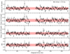 |
Fig. 1. NuSTAR FPMA+B light curves in the 3−79 keV, 3−10 keV, and 10−79 keV energy bands are shown in the top panels, with a binning time of 3.5 ks. The hardness ratio is shown in the bottom panel. Red shaded regions indicate mean count rates and hardness ratio ±1σ. |
2.3. Palomar
An optical observation of the source, quasi-simultaneous to the NuSTAR pointing, was performed using the Double Spectrograph (DBSP) on the Hale 200″ Telescope at the Palomar Observatory on 2021 March 18. We obtained a single 300 s observation (PI: D. Stern) at the parallactic angle through the 1.5″ slit in photometric, good-seeing conditions. Data were flux calibrated (but not corrected for telluric absorption) using spectrophotometric standard stars.
3. X-ray spectroscopy
3.1. 3–10 keV data analysis
We start our analysis by fitting the pn, MOS12, and FPMA and FPMB spectra of the source in the 3−10 keV energy band. The model is composed of an absorbed redshifted power law (TBABS × ZPOW in XSPEC) to reproduce the nuclear continuum, assuming a Galactic column density NH = 3.43 × 1020 cm−2 (HI4PI Collaboration 2016). Three multiplicative constants are included in the fit to take into account cross-calibration uncertainties between the pn and MOS12 detectors and flux variations between the 2014 and 2021 XMM and NuSTAR pointings. We obtain χ2/d.o.f. = 469/357 and no statistically significant change of the photon index between the four spectra is found. As large residuals can be seen in the observed 4−5.5 keV energy band, we included three narrow redshifted Gaussian lines to reproduce the fluorescence Fe, Kα, and Kβ emission lines and the highly ionized Fe XXV/XXVI Kα lines. The final best-fit χ2/d.o.f. is 318/348 and best fitting values can be found in Table 1. Figure 2 shows the best fit model, data, and residuals between 3 and 10 keV. While the first two emission lines at  keV and
  keV can be readily identified as neutral Fe Kα and Fe XXV He-α, the third one could be a blend of Fe XXVI Ly-α and the fluorescence Fe Kβ lines. The expected Fe Kβ/Fe Kα (core only) ratio ranges from 0.155 to 0.16 (Molendi et al. 2003) and we find Fe Kβ/Fe K
 . Given the large uncertainties, a possible contamination from Fe XXVI Ly-α cannot be discarded. Leaving the width of the neutral Fe Kα emission line free to vary does not lead to a statistically significant improvement of the fit (Δχ2/d.o.f. = −3/1) and an upper limit σ < 95 eV is obtained. The best fitting values for the equivalent width of the Fe Kα are EW = 55 ± 6 eV and EW = 38 ± 30 eV for the 2014 XMM and 2021 NuSTAR observations, respectively. Once the 3−10 keV best fitting model is applied to the 2008 pn snapshot, a good fit is obtained (χ2/d.o.f. = 85/73) and an EW = 100 ± 60 eV is retrieved, in agreement with (Krumpe et al. 2010). The equivalent width of the emission lines is calculated via the EQW command in XSPEC. As the uncertainties on the energy centroids and normalizations drive the total uncertainty on the EW value, we now show in Fig. 3 the contour plots between the Fe Kα energy centroid and normalization when these parameters are left free between the three epochs (solid and dashed lines indicate 68% and 90% confidence levels, respectively).
Best-fit parameters of the 3−10 keV fit of the joint XMM+NuSTAR data.
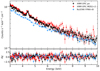 |
Fig. 2. Best fit in the 3−10 keV band. FPMA/B data are co-added for the sake of visual clarity using the SETPLOT GROUP command in XSPEC. |
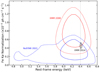 |
Fig. 3. Contour plots between the energy centroid and normalization of the Fe Kα emission line, for the three epochs. Solid and dashed lines indicate 68% and 90% confidence level contours, respectively. |
3.2. 0.3–79 keV data analysis
We then extended the energy band including low- and high-energy data and re-fitted with the baseline model composed of an absorbed power law and three Gaussians. The resulting χ2/d.o.f. is good (1033/713 = 1.45) but some residuals can still be seen in the 3−10 keV band and at high energies. We therefore included a Compton reflection component (modeled with PEXRAV in XSPEC: Magdziarz & Zdziarski 1995), abundances were fixed to the solar values, and the cosine of the inclination angle with respect to our line of sight was fixed to cosθ = 0.45. The final χ2/d.o.f. is 908/712 = 1.27 and a Compton reflection fraction R = 0.55 ± 0.10 is inferred, with a photon index Γ = 1.77 ± 0.01. The best-fit model and data are shown in Fig. 4. As some residuals are still present between the 1 and 4 keV bands, we considered a toroidal model to reproduce the reflection component.
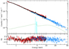 |
Fig. 4. Best-fit model, data, and residuals with PEXRAV model; see text for details. Color coding for the different instruments follows the same scheme used in Fig. 1. Clear residuals emerge at low energies. |
We removed the two Gaussians accounting for the Fe Kα and Fe Kβ lines and PEXRAV for the associated Compton reflection continuum, and XSPEC tables generated with the Monte Carlo radiative transfer code BORUS (Baloković et al. 2018, 2019) were included in the model. Different geometrical configurations for the circumnuclear material and physical assumptions on the input continuum can be tested. For the case of RBS 1055, we first consider two separate tables (BORUS02_V170323K.FITS and BORUS02_V170323L.FITS), one for the Compton reflection continuum and the other one for the associated emission lines. Furthermore, as no evidence for neutral absorption in excess of the Galactic one has yet been found (Krumpe et al. 2010), we assume two separate column densities for the absorber along the line of sight and for the scattering reflector. In particular, this is considered to be a sphere with conical cutouts at its poles, approximating a torus with variable covering factor. The half-opening angle of the polar cutouts, defined as θtor, is measured from the symmetry axis toward the equator, and ranges from 0° (which is a full covering sphere) to 83° (corresponding to a disk-like configuration covering 10% of the solid angle). In XSPEC, the model reads:
A constant covering factor of the torus Ctor = cos(θtor)=0.5 was assumed in this geometrical configuration. Normalizations, column densities, inclination angles, and constants were linked between the two BORUS tables. Photon indices, cutoff energies, and normalization were instead linked to the those of the cutoff power law. A best-fit χ2/d.o.f. = 719/715 = 1.01 was retrieved and best fitting parameters are reported in Table 2. Figure 5 shows the best-fit models, data, and corresponding residuals. The contour plots between the column density of the reflector and the high-energy cutoff EC are shown in Fig. 6. A Compton-thin solution is preferred for the toroidal reprocessor and a column density  cm−2 is measured. The primary continuum is well modeled with a power-law component with
  and EC > 110 keV. We note that the overall geometry of the torus is not self-consistent. The current configuration assumes θtor = 60° and θinc > 70°, allowing our line sight to intercept part of the toroidal structure. However, we only retrieve an upper limit NH < 5 × 1020 cm−2 for the column density of an absorber covering the primary power law. If we impose θinc < θtor in the model, a poorer fit (Δχ2 = +14) is obtained, with no statistically significant variation of best fitting parameters.
Best-fit parameters of the joint XMM+NuSTAR data analysis obtained with the BORUS component for the Compton reflection.
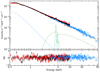 |
Fig. 5. Best-fit model, data, and residuals with the BORUS model; see text for details. Color coding for the different instruments follows the same scheme used in Fig. 1. |
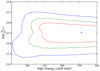 |
Fig. 6. Contour plots between the column density of the reflector NH and the high-energy cutoff EC obtained with BORUS model. Red, green, and blue solid lines indicate 68%, 90%, and 99% confidence levels, respectively. |
Following Krumpe et al. (2010), we checked for a soft excess component extending over the energy range of the pn-MOS spectra down to 0.3 keV, and therefore the final fit is between 0.3 and 79 keV. The resulting residuals were accounted for by an additional ZPOWERLAW component in XSPEC, which largely improves the fit (Δχ2/d.o.f. = −67/−2), for a final χ2/d.o.f. = 763/736 = 1.03. Some residuals are still present around ∼0.6 keV and the addition of an absorption line at E = 0.88 ± 0.03 keV with normalization N = ( − 1.3 ± 0.3)×10−5 ph cm−2 s−1 improves the fit (Δχ2/d.o.f. = −21/−2). However, this absorption feature is detected in the EPIC-pn spectrum only, and if a warm absorber component is included in the model (ZXIPCF in XSPEC), only a marginal improvement of the overall fit is found (χ2/d.o.f. = 751/734). The best fitting column density and ionization parameter are NH < 8 × 1021 cm−2 and  .
.
We then fixed the inclination angle, the photon index, and the high-energy cutoff of the reflection component to the best fitting ones, removed the soft and hard power laws, and included the Comptonization model NTHCOMP (Zdziarski et al. 1996; Życki et al. 1999). The temperature of the blackbody component kTBB is fixed to 5 eV, assuming a black hole mass MBH = 6.5 × 10⁸ M⊙. We have two different components, one for the soft excess and the other one for the hard power-law continuum. We substituted the two BORUS tables with the BORUS12_V190815A.FITS one, in which the intrinsic continuum is based on the NTHCOMP component and both the Compton-scattered continuum and emission lines are included. The final XSPEC model reads:
A photon index ΓW = 3.30 ± 0.37 and a temperature  keV are inferred for the soft Comptonization component while ΓH = 1.75 ± 0.01 and
  keV are found for the hard one, with a resulting χ2/d.o.f. = 765/740 = 1.03. These two pairs of values can be translated into optical depths, τ, using relation (1) in Marinucci et al. (2019), leading to Thomson optical depths
  and
and  for the warm and hot coronal components, respectively. The final best fitting model is shown in Fig. 7, in which OM data points are also included. The three main components of the model can be clearly seen: while the warm (in blue) and hot (in orange) coronae account for the power-law like continua from the UV to the hard X-rays, the Compton-thin reflector (in green) reproduces the Fe Kα and its associated continuum. Figure 8 shows the contour plots between the photon indices and the temperatures obtained, using 68% confidence levels. Gray data points are the best fitting values taken from Petrucci et al. (2018) for a sample of 22 radio-quiet AGN.
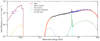 |
Fig. 7. The total best fitting model is shown as a red solid line and UV/X-ray data are superimposed. The four spectral components are labeled and shown as dashed lines. XMM-Newton OM data are plotted in purple, pn data in grey and NuSTAR grouped FPMA/B data in blue. Data have been rebinned in energy for the sake of visual clarity. |
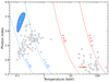 |
Fig. 8. Contour plots obtained with two NTHCOMP components for the warm and hot coronae are shown in blue and red, respectively. Shaded regions indicate 68% confidence levels. Dashed red and blue lines indicate different Thomson optical depths obtained with the formula (A1) in Zdziarski et al. (1996). Gray circles and diamonds are data points reported in Petrucci et al. (2018) for their sample of 22 sources. |
4. Optical spectroscopy
4.1. Data analysis
The red and blue channels of DBSP cover the MgII, Hβ, [OIII] doublet, and Hα emission lines. To model the line profiles, we fitted the emission lines separately with one or two Gaussian components with a local continuum characterization described by a power-law function, as shown in Fig. 9. Specifically, (a) the MgII line is modeled with a broad Gaussian component to describe the emission from the broad line region (BLR), and the adjacent wavelength range, which is contaminated by FeII multiplets, is modeled with FeII templates from Popović et al. (2019), which are convolved with a Gaussian function with a full-width half maximum (FWHM) in the range 1000−5000 km s−1; and (b) Hβ and [OIII] doublet lines are modeled with one Gaussian component to reproduce the systemic emission from the narrow line region (NLR) and an additional Gaussian function for any possible blueshifted or asymmetric emission associated with an outflowing gas. Moreover, we added a broad Gaussian component for the Hβ line to reproduce the emission from the BLR. Finally, (c) the Hα, [NII]6548,6583 Å emission line doublet and [SII] doublet are modeled similarly, that is, with two Gaussian components, systemic plus any contribution from the outflowing gas, and a broad Gaussian component for Hα originating in the BLR.
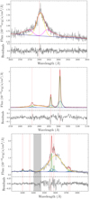 |
Fig. 9. Optical spectroscopy. (a) The MgII line spectrum, (b) Hβ-[OIII] region and (c) Hα-[SII] region. The red curves represent the best-fit models. Gold Gaussian components represent the emission originating from the BLR, the magenta curve refers to the iron emission and navy blue power-law curves represent the continuum emission. Green Gaussian components reproduce the NLR emission and blue ones trace the outflowing gas in the NLR. Dashed vertical red lines indicate the location of the emission lines of interest at the systemic redshift. The vertical grey shaded region marks the channels affected by telluric absorptions which were masked during the fitting procedure. |
The centroids and the velocity dispersion of similar components are tied together. Further, the outflow components of the Hα + [NII] + [SII] system have the same velocity dispersion as the [OIII] outflow component in order to avoid degeneracy. [NII]6548 Å/[NII]6583 Å and [OIII]5007 Å/[OIII]4959 Å flux ratios were fixed to 3 based on the atomic transition probability (Osterbrock & Ferland 2006). We modeled the FeII emission with the observational templates of Boroson & Green (1992), Véron-Cetty et al. (2004), and Tsuzuki et al. (2006), but we do not detect a strong FeII component in the region of Hβ. The best-fit model is chosen with a χ2 minimization process. The best fitting parameters are presented in Table 3, and the best-fit models in Fig. 9. The uncertainties of free parameters are calculated using a Monte-Carlo approach: we added random Gaussian noise to the best-fit model with dispersion equal to the rms of the spectrum and repeated the fit 1000 times. The associated errors are estimated using the 84th and 16th percentiles of the parameter distribution.
[OIII]λ5007 emission line properties.
4.2. Continuum and emission line luminosity
From the emission line modeling, we derived a more accurate estimate of the redshift by adopting the [OIII]λ5007 narrow component (z = 0.452 ± 0.001) as the systemic line. We find that the Hβ BLR line centroid is redshifted with respect to the expected line position (4862 Å) of ΔvHβ = 1500 ± 100 km s−1 and the BLR Hβ line luminosity is  = 1.56 ± 0.07 × 1043 erg s−1. Similarly, we obtain a BLR Hα line luminosity
  = 1.11 ± 0.03 × 1044 erg s−1 and a redshifted centroid value that is consistent with that found for the BLR component of Hβ (ΔvHα = 1600 ± 100 km s−1). We computed the observed Balmer decrement, defined as the line ratios of BLR Hα/Hβ and find a value of 7.08 ± 0.18.
Baron et al. (2016), analyzing a sample of ∼5000 Type 1 AGN at z ∼ 0.4, found a mean Hα/Hβ ∼ 3 with a broad distribution in the range 1.5−4, suggesting that Case B recombination cannot explain the ratio in all sources. We calculated the optical reddening as E(B − V)=1.97 × log10((Hα/Hβ)/(Hα/Hβ)intrinsic) (Osterbrock 1989), where the intrinsic Balmer decrement is assumed to be 3 (Baron et al. 2016) and derived E(B − V)=0.73. However, when comparing the optical spectrum of our target with that of the composite AGN spectrum of Vanden Berk et al. (2001), we find no extinction for the continuum, confirming that our target has a blue optical continuum (see Sect. 5 for a discussion).
For the NLR, we find Hα/Hβ = 5.4 ± 0.4, which is lower than the BLR value but still larger than the intrinsic Balmer ratio for a low-density environment such as the NLR, 2.74−2.86, assuming case B recombination (Osterbrock & Ferland 2006). The lower value found for the NLR suggests a different level of reddening in the two regions and may imply that the extinction of the BLR is due to dusty structures that are more compact than the NLR.
4.3. BH mass and Eddington ratio
Single-epoch BH masses are usually estimated for Type 1 AGN from the broad emission lines (e.g., Greene & Ho 2007; Vestergaard & Osmer 2009). Assuming that the BLR clouds are in virial motion, the BH mass is proportional to RV2/G, with R being the radius of the BLR and V the gas velocity. These two parameters can be estimated from the width of the broad emission lines and the radius from the radius–luminosity relation defined by reverberation mapping (e.g., Bentz et al. 2013). From the best-fitting results, we calculated the monochromatic luminosity at 3000 Å (L3000 = 9.8 ± 0.16 × 1044 erg s−1) and 5100 Å (L5100 = 8.10 ± 0.06 × 1044 erg s−1), and the Hα BLR line luminosity (see Table 4) as well as the FWHM of Hβ, Hα, and MgII lines to derive the BH mass estimated using the calibration of Bongiorno et al. (2014) for Hβ and MgII and that of Greene & Ho (2005) for Hα. We find a BH mass in the range 2.79 × 10⁸ − 1.19 × 10⁹ M⊙, according to different BLR emission lines, with an average value of ⟨MBH⟩=6.52 × 10⁸ M⊙, which we use as our preferred value hereafter.
BLR properties from MgII, Hβ, and Hα emission lines.
We estimated the bolometric luminosity of the AGN assuming a bolometric correction factor for the continuum luminosity λ5100L5100, adopting the prescription proposed by Saccheo et al. (in prep.) of K5100 Å ∼ 4.80 ± 1.54, and find LBol = 3.86 × 1045 erg s−1. From the BH mass and bolometric luminosity, it is possible to estimate the Eddington ratio defined as λEdd = LBol/LEdd, and we find λEdd = 0.05 by assuming ⟨MBH⟩.
4.4. Outflow properties
We traced the outflow in the NLR in its warm ionized phase using the [OIII]5007 emission line, because it is sensitive to the gas temperature and ionization parameter. Previous works alternatively used the Hβ line (e.g., Liu et al. 2013; Harrison et al. 2014); however, in our case, the Hβ line is mostly dominated by the component arising from the BLR gas, and therefore the [OIII] is the preferred outflow tracer.
We estimated the outflowing gas mass Mout and mass outflow rate Ṁout following the method presented in Bischetti et al. (2017), assuming a spherically or biconically symmetric mass-conserving free wind with mass-outflow rate and velocity that are independent of radius (Rupke et al. 2002, 2005), and assuming that most of the oxygen consists of [OIII] ions. We used the relation by Carniani et al. (2015) and derive the outflowing ionized gas mass from the luminosity associated with the broad [OIII] emission:
![Mathematical equation: $$ \begin{aligned} \log \frac{M_{\rm out}}{M_{\odot }} =&7.6 + {\log \left(\frac{C}{10^{\mathrm{[O/H]{-}[O/H]}_{\odot }}}\right)} + \log \left(\frac{L_{\rm [OIII]}^\mathrm{out}}{10^{44}\,\mathrm{erg\,s}^{-1}}\right)\nonumber \\ &\pm \log \left(\frac{\langle n_{\rm e}\rangle }{10^3\,\mathrm{cm}^{-3}}\right), \end{aligned} $$](/articles/aa/full_html/2022/10/aa44272-22/aa44272-22-eq41.gif) (1)
(1)
where  , [O/H]−[O/H]⊙ is the gas metallicity relative to the solar value,
 ![Mathematical equation: $ L^{\mathrm{out}}_{\mathrm{[OIII]}} $](/articles/aa/full_html/2022/10/aa44272-22/aa44272-22-eq43.gif) is the outflowing [O III]5007 luminosity, and ⟨ne⟩ is the average electron density. This last parameter can be estimated from the line ratio of the [SII]λ6716,6731 doublet (Peterson 1997) of the outflowing component. Assuming an electron temperature of ∼104 K, which is a typical value for AGN outflows (e.g., Perna et al. 2017 and references therein), we find a value of ne ≅ 177 cm−3. Assuming a solar metallicity and C ≈ 1, we derived Mout = 2.84 × 10⁷ M⊙. We note that this measurement strongly depends on the electron density. We also derived the mass outflow rate Ṁout from the fluid-field continuity equation for a local estimate of the mass rate at a given radius, as follows:
is the outflowing [O III]5007 luminosity, and ⟨ne⟩ is the average electron density. This last parameter can be estimated from the line ratio of the [SII]λ6716,6731 doublet (Peterson 1997) of the outflowing component. Assuming an electron temperature of ∼104 K, which is a typical value for AGN outflows (e.g., Perna et al. 2017 and references therein), we find a value of ne ≅ 177 cm−3. Assuming a solar metallicity and C ≈ 1, we derived Mout = 2.84 × 10⁷ M⊙. We note that this measurement strongly depends on the electron density. We also derived the mass outflow rate Ṁout from the fluid-field continuity equation for a local estimate of the mass rate at a given radius, as follows:
 (2)
(2)
where vmax is the outflow velocity defined as ![Mathematical equation: $ |\Delta v|^{\mathrm{out}}_{\mathrm{[OIII]}} + 2\sigma_{\mathrm{[OIII]}}^{\mathrm{out}} $](/articles/aa/full_html/2022/10/aa44272-22/aa44272-22-eq45.gif) ([OIII] |Δv| is the velocity shift between narrow and outflow [OIII] emission centroids and σ is the velocity dispersion of the [OIII] outflow component) and Rout is the spatial extent of the outflow. As we do not have spatial information, we assumed Rout = 4.4 kpc, equal to the half-slit width. From the best fitting model parameters, we derived the velocity shift and velocity dispersion of the outflow component, and therefore vmax, as reported in Table 3. In this way, we obtained Ṁout ∼ 25 M⊙ yr−1. From Ṁout, we then derived the kinetic power associated with the outflow,
([OIII] |Δv| is the velocity shift between narrow and outflow [OIII] emission centroids and σ is the velocity dispersion of the [OIII] outflow component) and Rout is the spatial extent of the outflow. As we do not have spatial information, we assumed Rout = 4.4 kpc, equal to the half-slit width. From the best fitting model parameters, we derived the velocity shift and velocity dispersion of the outflow component, and therefore vmax, as reported in Table 3. In this way, we obtained Ṁout ∼ 25 M⊙ yr−1. From Ṁout, we then derived the kinetic power associated with the outflow,  , and find a value of 1.3 × 1043 erg s−1, corresponding to a coupling efficiency with the interstellar medium
  /LBol ≈ 0.33%. Theoretical models predict a coupling of 0.1%–5% for AGN-driven outflows (King 2005). The value found for RBS 1055 might be sufficient for an efficient feedback mechanism, which will affect the gas content and star formation rate in the host galaxy. However, IFU spectroscopy is necessary to accurately determine the exact extension of the outflow and the spatial distribution of the density of the outflowing gas. We note that, given the typical multi-phase nature of AGN-driven outflows (Cicone et al. 2018; Bischetti et al. 2019; Fluetsch et al. 2021), the derived
  should be considered as a fraction of the total kinetic power of the outflow in RBS 1055 including all gas (i.e., molecular and atomic) phases.
5. Discussion
In the sections above, we report our analysis of long observations of the bright quasar RBS 1055 with XMM-Newton in 2014 and with NuSTAR in 2021. A ∼10% drop in the 2−10 keV flux (1.38−6.88 keV at the rest-frame of the source) is observed after seven years, from F2 − 10 = (2.7 ± 0.1)×10−12 erg cm−2 s−1 to F2 − 10 = (2.4 ± 0.2)×10−12 erg cm−2 s−1. At the redshift of the source, these fluxes correspond to L2 − 10 = (2.0 ± 0.2)×1045 erg s−1 and L2 − 10 = (1.8 ± 0.2)×1045 erg s−1, respectively. Assuming a black hole mass estimate of MBH = 6.5 × 10⁸ M⊙ (see Sect. 4.3) and adopting the bolometric corrections KX(LX) from Duras et al. (2020, Eq. (3)), we retrieve bolometric luminosities LBol = 7.4 × 1046 erg s−1 and 6.4 × 1046 erg s−1 for the 2014 and 2021 epochs, respectively. The corresponding accretion rates are λEdd = 0.9 and λEdd = 0.8, respectively. The 2021 bolometric luminosity calculated from the 2−10 keV luminosity is a factor ∼15 higher than the one estimated from the continuum luminosity at 5100 Å. An important proxy of the interaction between the accretion disk and the corona is the slope of the power law connecting the rest-frame X-ray luminosity at 2 keV and the rest-frame UV luminosity at 2500 Å, that is, αox = 0.384 log(L2500 Å/L2 keV) (Tananbaum et al. 1979; Steffen et al. 2006; Just et al. 2007; Lusso et al. 2010; Lusso & Risaliti 2017; Risaliti & Lusso 2019). Interpolating the UV luminosities inferred with the UVW1 (2910 Å) and U (3440 Å) filters, we obtain a monochromatic 2500 Å luminosity  and, using the best fit discussed in Sect. 3.2, a 2 keV luminosity
  . We therefore infer an αox = 1.06. This value lies at the very low end of the αox distribution obtained from high-redshift quasar samples. If compared with the WISSH (WISE-SDSS selected hyper-luminous) quasars (z ∼ 1.8 − 4.8, Bischetti et al. 2017), using the best fitting relation (3) in Martocchia et al. (2017), we obtain a difference Δαox = 0.39. From Eq. (8) in Vagnetti et al. (2013), in which Swift observations of sources at z ∼ 0.01 − 0.4 are considered, we find Δαox = 0.35. Applying the LX − LUV relation reported in Risaliti & Lusso (2019) to the measured monochromatic 2500 Å luminosity, a
  is retrieved, which is well below the
  observed value. This difference is in agreement with the one between the bolometric luminosities discussed above. We therefore conclude that RBS 1055, despite a ∼10% decrease in the total 2−10 keV flux in 2021, continues to have an extremely X-ray-bright SED, which is 10−15 times higher than other objects in this redshift range.
Detections of Compton reflection features are very scarce and such features are poorly constrained in luminous AGN because they are typically derived from 0.5−10 keV spectra. They seem to suggest low values of the Compton reflection fraction R, namely much lower than unity (Reeves & Turner 2000; Page et al. 2005), even when NuSTAR observations are taken into account (Zappacosta et al. 2018). An anti-correlation exists between the EW of the narrow neutral Fe Kα line and L2 − 10 keV (e.g., the IT effect; Iwasawa & Taniguchi 1993; Page et al. 2004; Bianchi et al. 2007). The IT effect is interpreted in terms of a decreasing covering factor of the Compton-thick toroidal reflector as a function of the increasing L2 − 10. However, the quality of the data for objects with L2 − 10 > 1045 erg s−1 is typically too poor even to put tight constraints on the EW of the Fe Kα line (Jiménez-Bailón et al. 2005). RBS 1055 is a clear outlier of this observed correlation: considering the best fitting EW–L2 − 10 keV relation in Bianchi et al. (2007) for radio-quiet sources, we measured an Fe Kα EW which is ∼3σ above the EW = 32 eV predicted value. However, this difference reduces to ∼2σ if their EW–λEdd relation is considered. This suggests that, despite the high luminosity, the circumnuclear reflector still covers a large solid angle and is found to be Compton-thin (with an equatorial column density  cm−2). Our best-fit model, using BORUS, does not constrain the covering factor of the torus because we only retrieve θtor > 50° when this parameter is left free (for an improvement of the fit Δχ2 = −7 with one additional degree of freedom). This suggests that the circumnuclear torus in RBS 1055 is likely to be clumpy, as already observed in some local sources (Uematsu et al. 2021; Marinucci et al. 2016). Even though only Compton-thick candidates were considered, according to recent NuSTAR samples (Brightman et al. 2015; Marchesi et al. 2019), this is the first tentative measurement of a torus covering factor above 1045 erg s−1.
In the last few years, high-quality Chandra data have shown that the Fe Kα can be spatially extended both in Compton-thin (Yi et al. 2021) and in Compton-thick galaxies (Marinucci et al. 2012; Fabbiano et al. 2017; Jones et al. 2021). The projected distances range from tens of parsecs (as in the Circinus galaxy: Marinucci et al. 2013) up to kiloparsec scale (as in NGC 1068: Young et al. 2001). Furthermore, a role of reflection in the host galaxy scale was recently discussed in Yan et al. (2021). In RBS 1055, if a fraction of the Fe Kα emission line is produced from material located lightyears away from the X-ray source, this could echo the higher intrinsic flux of the source observed in recent years.
Total mid-infrared (MIR) luminosities of the source, obtained with the Wide-Field Infrared Survey Explorer (WISE), were reported by Ichikawa et al. (2017, indicated as 2MASSi J1159410−195924):  ,
,  , and
, and  . The observed luminosity at 12 μm is in agreement with those estimated using the L12 μm − L2 − 10 keV correlations from Gandhi et al. (2009) and Asmus et al. (2015), within statistical uncertainties. In the latter work, local AGN (z < 0.3) in the luminosity range
  were considered. The MIR colors can also be used to estimate the amount of obscuration along the line of sight, as discussed in Pfeifle et al. (2022). Using Eq. (3) of this latter publication, from the ratio L22 μm/L4.6 μm = 1.17 we obtain a column density value in agreement with the upper limit found in Sect. 3.2 here. However, the obscuring column is known to correlate with the L2 − 10 keV/L12 μm ratio (Ichikawa et al. 2012; Yan et al. 2019). Equation (1) in Pfeifle et al. (2022) allows us to estimate the 2−10 keV luminosity from the inferred upper limit NH < 5 × 1020 cm−2. We find
  i.e., L2 − 10 keV ≃ 2.6 × 1045 erg s−1, which supports the scenario in which the intrinsic flux of the source has been steadily decreasing over the years.
The broad band emission of RBS 1055 can be well described in terms of the two-corona model. A warmer population of electrons ( keV) with a Thomson optical depth
  is responsible for the soft excess below ∼1 keV and for the optical and UV emission, while a second, hotter corona (
 keV) with
  accounts for the high-energy spectral shape. These values are in agreement with those discussed in Petrucci et al. (2018) for a wider sample of radio-quiet AGN. The sample studied by these latter authors includes only one source at a redshift z > 0.4 (namely HB 890405−123, at z = 0.5725) and RBS 1055 therefore provides further confirmation of this model at high redshifts. As opposed to Middei et al. (2020) and Ursini et al. (2020), we find that, for the cases of Mrk 359 and HE 1143−1810, respectively, a contribution from relativistic reflection off the inner regions of the accretion disk is unlikely, because a broad Fe Kα component is not found. We note that the inferred values for the high-energy cutoff and for the temperature of the hot corona follow the EC ≃ (2 − 5)kTe trend (Middei et al. 2019).
As reported in Sect. 4.2, by analyzing the optical spectrum of RBS 1055, we find a very high Balmer decrement for the BLR emission, which is indicative of reddening in this region. An excess of optical reddening has been observed in several other AGN (Barcons et al. 2003; Pappa et al. 2001; Carrera et al. 2004; Corral et al. 2005). The explanations suggested for this behavior are related to (i) the presence of a dusty warm absorber and (ii) an intrinsic property of the BLR. The first hypothesis could partially explain our findings, as the presence of a warm absorber is marginally detected in RBS1055 (see Sect. 3). The very high Balmer decrement could also suggest that case B recombination is not always valid in the BLR, and therefore it could be an intrinsic property of the BLR, or is the result of a peculiar geometry according to which our line of sight intercepts dust that reddens the BLR emission but not the optical continuum.
Such dust layers partially obscuring the BLR could be located between the BLR probed by the Balmer and the MgII lines, as the latter is only slightly redshifted (ΔvMgII = 480 ± 100 km s−1). To examine how our target relates to the bulk of the SDSS AGN population, we compared the measured Hα/MgII and Hβ/MgII line ratios of our target with those from the catalogue of Shen et al. (2011), finding no difference with the majority of SDSS AGN, while the Hα/Hβ ratio falls in the tail of the SDSS Hα/Hβ ratio distribution. No peculiar properties are found when considering the relation between X-ray luminosity and Balmer lines, as shown in Fig. 10. Here the Balmer decrement is shown as a function of the LX/LHβ ratio for a large sample of Seyfert 1 galaxies from Ward et al. (1988), who found that the differences in the Balmer decrements are due to reddening rather than to an intrinsic property of the BLR. RBS 1055 appears to be consistent with the trend reported in Fig. 10, which supports the hypothesis of nuclear reddening.
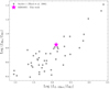 |
Fig. 10. Correlation between Log (LHα/LHβ) and Log (LX/LHβ). Magenta star represents RBS 1055 values, while gray dots refer to Seyfert 1 sample from Ward et al. (1988). |
6. Conclusions
We analyzed and discussed the novel NuSTAR observation of RBS 1055 performed in March 2021 and the archival XMM-Newton pointings taken in July 2014. An optical spectrum of the source taken with the Double Spectrograph at the Palomar Observatory was also studied. Our main results can be summarized as follows:
– We confirm the presence of an intense Fe Kα emission line at  keV, with EW = 55 ± 6 eV. This measurement is ∼3σ above the predicted value from the observed EW–L2 − 10 keV relation (Bianchi et al. 2007) and represents one of the few above L2 − 10 keV = 1045 erg s−1 with a robust Fe Kα line. Once a toroidal model is considered to model the Compton reflection, a column density
  cm−2 is retrieved.
– The primary nuclear continuum is well modeled with a cutoff power law with  , EC > 110 keV and a soft excess component is present in the pn/MOS spectra. We find that the two-corona model (Petrucci et al. 2013, 2018) reproduces the broad band spectrum of RBS 1055 well, with temperatures
  keV and
  keV and Thomson optical depths
  and
and  for the warm and hot coronal components, respectively.
– We also confirm that the source has an extremely X-ray-bright SED, with an inferred αox = 1.06. This value is at the lower end of the observed αox distributions (Martocchia et al. 2017; Vagnetti et al. 2013).
– The optical spectrum reveals a likely peculiar configuration of our line of sight with respect to the nucleus, and the presence of a broad [O III] component, tracing outflows in the NLR, with a velocity shift v = 1500 ± 100 km s−1, leading to a Ṁout = 25.4 ± 1.5 M⊙ yr−1 and  % (adopting the 5100 Å-based LBol value).
Acknowledgments
We thank the anonymous referee for their comments and suggestions, which greatly improved the paper. A.M., G.V., E.P., S.B., G.L., and C.V. acknowledge support from PRIN MIUR project “Black Hole winds and the Baryon Life Cycle of Galaxies: the stone-guest at the galaxy evolution supper”, contract no. 2017PH3WAT. G.V. and E.P. acknowledge financial support under ASI-INAF contract 2017-14-H.0. We made use of ASTROPY (http://www.astropy.org), a community-developed core PYTHON package for Astronomy (Astropy Collaboration 2013, 2018) and MATPLOTLIB (Hunter 2007). This research has made use of the NuSTAR Data Analysis Software (NuSTARDAS) jointly developed by the ASI Science Data Center (ASDC, Italy) and the California Institute of Technology (USA).
References
- Arnaud, K. A. 1996, ASP Conf. Ser., 101, 17 [Google Scholar]
- Arnaud, K. A., Branduardi-Raymont, G., Culhane, J. L., et al. 1985, MNRAS, 217, 105 [NASA ADS] [CrossRef] [Google Scholar]
- Asmus, D., Gandhi, P., Hönig, S. F., Smette, A., & Duschl, W. J. 2015, MNRAS, 454, 766 [NASA ADS] [CrossRef] [Google Scholar]
- Astropy Collaboration (Robitaille, T. P., et al.) 2013, A&A, 558, A33 [NASA ADS] [CrossRef] [EDP Sciences] [Google Scholar]
- Astropy Collaboration (Price-Whelan, A. M., et al.) 2018, AJ, 156, 123 [Google Scholar]
- Baloković, M., Brightman, M., Harrison, F. A., et al. 2018, ApJ, 854, 42 [Google Scholar]
- Baloković, M., García, J. A., & Cabral, S. E. 2019, Res. Notes Am. Astron. Soc., 3, 173 [Google Scholar]
- Baloković, M., Harrison, F. A., Madejski, G., et al. 2020, ApJ, 905, 41 [Google Scholar]
- Barcons, X., Carrera, F. J., & Ceballos, M. T. 2003, MNRAS, 339, 757 [NASA ADS] [CrossRef] [Google Scholar]
- Baron, D., Stern, J., Poznanski, D., & Netzer, H. 2016, ApJ, 832, 8 [Google Scholar]
- Beloborodov, A. M. 1999, ASP Conf. Ser., 161, 295 [Google Scholar]
- Bentz, M. C., Denney, K. D., Grier, C. J., et al. 2013, ApJ, 767, 149 [Google Scholar]
- Bertola, E., Vignali, C., Lanzuisi, G., et al. 2022, A&A, 662, A98 [NASA ADS] [CrossRef] [EDP Sciences] [Google Scholar]
- Bianchi, S., Guainazzi, M., Matt, G., & Fonseca Bonilla, N. 2007, A&A, 467, L19 [NASA ADS] [CrossRef] [EDP Sciences] [Google Scholar]
- Bischetti, M., Piconcelli, E., Vietri, G., et al. 2017, A&A, 598, A122 [NASA ADS] [CrossRef] [EDP Sciences] [Google Scholar]
- Bischetti, M., Piconcelli, E., Feruglio, C., et al. 2019, A&A, 628, A118 [NASA ADS] [CrossRef] [EDP Sciences] [Google Scholar]
- Bongiorno, A., Maiolino, R., Brusa, M., et al. 2014, MNRAS, 443, 2077 [NASA ADS] [CrossRef] [Google Scholar]
- Boroson, T. A., & Green, R. F. 1992, ApJS, 80, 109 [Google Scholar]
- Brightman, M., Baloković, M., Stern, D., et al. 2015, ApJ, 805, 41 [NASA ADS] [CrossRef] [Google Scholar]
- Carniani, S., Marconi, A., Maiolino, R., et al. 2015, A&A, 580, A102 [NASA ADS] [CrossRef] [EDP Sciences] [Google Scholar]
- Carrera, F. J., Page, M. J., & Mittaz, J. P. D. 2004, A&A, 420, 163 [NASA ADS] [CrossRef] [EDP Sciences] [Google Scholar]
- Cicone, C., Severgnini, P., Papadopoulos, P. P., et al. 2018, ApJ, 863, 143 [NASA ADS] [CrossRef] [Google Scholar]
- Corral, A., Barcons, X., Carrera, F. J., Ceballos, M. T., & Mateos, S. 2005, A&A, 431, 97 [NASA ADS] [CrossRef] [EDP Sciences] [Google Scholar]
- Done, C., Davis, S. W., Jin, C., Blaes, O., & Ward, M. 2012, MNRAS, 420, 1848 [Google Scholar]
- Duras, F., Bongiorno, A., Ricci, F., et al. 2020, A&A, 636, A73 [NASA ADS] [CrossRef] [EDP Sciences] [Google Scholar]
- Fabbiano, G., Elvis, M., Paggi, A., et al. 2017, ApJ, 842, L4 [NASA ADS] [CrossRef] [Google Scholar]
- Fabian, A. C., Lohfink, A., Kara, E., et al. 2015, MNRAS, 451, 4375 [Google Scholar]
- Fabian, A. C., Lohfink, A., Belmont, R., Malzac, J., & Coppi, P. 2017, MNRAS, 467, 2566 [Google Scholar]
- Fluetsch, A., Maiolino, R., Carniani, S., et al. 2021, MNRAS, 505, 5753 [NASA ADS] [CrossRef] [Google Scholar]
- Gabriel, C., Denby, M., Fyfe, D. J., et al. 2004, in Astronomical Data Analysis Software and Systems (ADASS) XIII, eds. F. Ochsenbein, M. G. Allen, & D. Egret, ASP Conf. Ser., 314, 759 [NASA ADS] [Google Scholar]
- Gandhi, P., Horst, H., Smette, A., et al. 2009, A&A, 502, 457 [NASA ADS] [CrossRef] [EDP Sciences] [Google Scholar]
- George, I. M., & Fabian, A. C. 1991, MNRAS, 249, 352 [Google Scholar]
- Greene, J. E., & Ho, L. C. 2005, ApJ, 630, 122 [NASA ADS] [CrossRef] [Google Scholar]
- Greene, J. E., & Ho, L. C. 2007, ApJ, 667, 131 [NASA ADS] [CrossRef] [Google Scholar]
- Haardt, F., & Maraschi, L. 1991, ApJ, 380, L51 [Google Scholar]
- Haardt, F., Maraschi, L., & Ghisellini, G. 1994, ApJ, 432, L95 [NASA ADS] [CrossRef] [Google Scholar]
- Harrison, F. A., Craig, W. W., Christensen, F. E., et al. 2013, ApJ, 770, 103 [Google Scholar]
- Harrison, C. M., Alexander, D. M., Mullaney, J. R., & Swinbank, A. M. 2014, MNRAS, 441, 3306 [Google Scholar]
- HI4PI Collaboration (Ben Bekhti, N., et al.) 2016, A&A, 594, A116 [NASA ADS] [CrossRef] [EDP Sciences] [Google Scholar]
- Hunter, J. D. 2007, Comput. Sci. Eng., 9, 90 [NASA ADS] [CrossRef] [Google Scholar]
- Ichikawa, K., Ueda, Y., Terashima, Y., et al. 2012, ApJ, 754, 45 [Google Scholar]
- Ichikawa, K., Ricci, C., Ueda, Y., et al. 2017, ApJ, 835, 74 [NASA ADS] [CrossRef] [Google Scholar]
- Iwasawa, K., & Taniguchi, Y. 1993, ApJ, 413, L15 [NASA ADS] [CrossRef] [Google Scholar]
- Jansen, F., Lumb, D., Altieri, B., et al. 2001, A&A, 365, L1 [NASA ADS] [CrossRef] [EDP Sciences] [Google Scholar]
- Jiang, P., Wang, J. X., & Wang, T. G. 2006, ApJ, 644, 725 [NASA ADS] [CrossRef] [Google Scholar]
- Jiménez-Bailón, E., Piconcelli, E., Guainazzi, M., et al. 2005, A&A, 435, 449 [NASA ADS] [CrossRef] [EDP Sciences] [Google Scholar]
- Jin, C., Ward, M., Done, C., & Gelbord, J. 2012, MNRAS, 420, 1825 [Google Scholar]
- Jones, M. L., Parker, K., Fabbiano, G., et al. 2021, ApJ, 910, 19 [NASA ADS] [CrossRef] [Google Scholar]
- Just, D. W., Brandt, W. N., Shemmer, O., et al. 2007, ApJ, 665, 1004 [Google Scholar]
- Kammoun, E. S., Risaliti, G., Stern, D., et al. 2017, MNRAS, 465, 1665 [CrossRef] [Google Scholar]
- Kawamuro, T., Ueda, Y., Tazaki, F., Ricci, C., & Terashima, Y. 2016, ApJS, 225, 14 [NASA ADS] [CrossRef] [Google Scholar]
- King, A. 2005, ApJ, 635, L121 [Google Scholar]
- Krumpe, M., Lamer, G., Markowitz, A., & Corral, A. 2010, ApJ, 725, 2444 [NASA ADS] [CrossRef] [Google Scholar]
- Lanzuisi, G., Gilli, R., Cappi, M., et al. 2019, ApJ, 875, L20 [Google Scholar]
- Lightman, A. P., & Zdziarski, A. A. 1987, ApJ, 319, 643 [NASA ADS] [CrossRef] [Google Scholar]
- Liu, G., Zakamska, N. L., Greene, J. E., Nesvadba, N. P. H., & Liu, X. 2013, MNRAS, 436, 2576 [NASA ADS] [CrossRef] [Google Scholar]
- Lubiński, P., Beckmann, V., Gibaud, L., et al. 2016, MNRAS, 458, 2454 [Google Scholar]
- Lusso, E., & Risaliti, G. 2017, A&A, 602, A79 [NASA ADS] [CrossRef] [EDP Sciences] [Google Scholar]
- Lusso, E., Comastri, A., Vignali, C., et al. 2010, A&A, 512, A34 [NASA ADS] [CrossRef] [EDP Sciences] [Google Scholar]
- Magdziarz, P., & Zdziarski, A. A. 1995, MNRAS, 273, 837 [Google Scholar]
- Magdziarz, P., Blaes, O. M., Zdziarski, A. A., Johnson, W. N., & Smith, D. A. 1998, MNRAS, 301, 179 [NASA ADS] [CrossRef] [Google Scholar]
- Marchesi, S., Ajello, M., Zhao, X., et al. 2019, ApJ, 872, 8 [Google Scholar]
- Marinucci, A., Risaliti, G., Wang, J., et al. 2012, MNRAS, 423, L6 [CrossRef] [Google Scholar]
- Marinucci, A., Miniutti, G., Bianchi, S., Matt, G., & Risaliti, G. 2013, MNRAS, 436, 2500 [CrossRef] [Google Scholar]
- Marinucci, A., Bianchi, S., Matt, G., et al. 2016, MNRAS, 456, L94 [Google Scholar]
- Marinucci, A., Porquet, D., Tamborra, F., et al. 2019, A&A, 623, A12 [NASA ADS] [CrossRef] [EDP Sciences] [Google Scholar]
- Martocchia, S., Piconcelli, E., Zappacosta, L., et al. 2017, A&A, 608, A51 [NASA ADS] [CrossRef] [EDP Sciences] [Google Scholar]
- Matt, G., Perola, G. C., & Piro, L. 1991, A&A, 247, 25 [NASA ADS] [Google Scholar]
- Middei, R., Bianchi, S., Marinucci, A., et al. 2019, A&A, 630, A131 [NASA ADS] [CrossRef] [EDP Sciences] [Google Scholar]
- Middei, R., Petrucci, P. O., Bianchi, S., et al. 2020, A&A, 640, A99 [NASA ADS] [CrossRef] [EDP Sciences] [Google Scholar]
- Molendi, S., Bianchi, S., & Matt, G. 2003, MNRAS, 343, L1 [Google Scholar]
- Osterbrock, D. E. 1989, Ann. N. Y. Acad. Sci., 571, 99 [NASA ADS] [CrossRef] [Google Scholar]
- Osterbrock, D. E., & Ferland, G. J. 2006, Astrophysics of Gaseous Nebulae and Active Galactic Nuclei (Sausalito: University Science Books) [Google Scholar]
- Page, K. L., O’Brien, P. T., Reeves, J. N., & Turner, M. J. L. 2004, MNRAS, 347, 316 [NASA ADS] [CrossRef] [Google Scholar]
- Page, K. L., Reeves, J. N., O’Brien, P. T., & Turner, M. J. L. 2005, MNRAS, 364, 195 [NASA ADS] [CrossRef] [Google Scholar]
- Pappa, A., Georgantopoulos, I., Stewart, G. C., & Zezas, A. L. 2001, MNRAS, 326, 995 [NASA ADS] [CrossRef] [Google Scholar]
- Perna, M., Lanzuisi, G., Brusa, M., Cresci, G., & Mignoli, M. 2017, A&A, 606, A96 [NASA ADS] [CrossRef] [EDP Sciences] [Google Scholar]
- Perola, G. C., Matt, G., Cappi, M., et al. 2002, A&A, 389, 802 [NASA ADS] [CrossRef] [EDP Sciences] [Google Scholar]
- Peterson, B. M. 1997, An Introduction to Active Galactic Nuclei (Cambridge: Cambridge University Press) [Google Scholar]
- Petrucci, P. O., Haardt, F., Maraschi, L., et al. 2000, ApJ, 540, 131 [Google Scholar]
- Petrucci, P. O., Haardt, F., Maraschi, L., et al. 2001, ApJ, 556, 716 [Google Scholar]
- Petrucci, P.-O., Paltani, S., Malzac, J., et al. 2013, A&A, 549, A73 [NASA ADS] [CrossRef] [EDP Sciences] [Google Scholar]
- Petrucci, P.-O., Ursini, F., De Rosa, A., et al. 2018, A&A, 611, A59 [NASA ADS] [CrossRef] [EDP Sciences] [Google Scholar]
- Pfeifle, R. W., Ricci, C., Boorman, P. G., et al. 2022, ApJS, 261, 3 [NASA ADS] [CrossRef] [Google Scholar]
- Piconcelli, E., Jimenez-Bailón, E., Guainazzi, M., et al. 2004, MNRAS, 351, 161 [Google Scholar]
- Popovi{\’c}, L., Kovačević-Dojčinović, J., & Marčeta-Mand ić, S. 2019, MNRAS, 484, 3180 [CrossRef] [Google Scholar]
- Porquet, D., Reeves, J. N., O’Brien, P., & Brinkmann, W. 2004, A&A, 422, 85 [NASA ADS] [CrossRef] [EDP Sciences] [Google Scholar]
- Reeves, J. N., & Turner, M. J. L. 2000, MNRAS, 316, 234 [NASA ADS] [CrossRef] [Google Scholar]
- Ricci, C., Ueda, Y., Paltani, S., et al. 2014, MNRAS, 441, 3622 [NASA ADS] [CrossRef] [Google Scholar]
- Ricci, C., Trakhtenbrot, B., Koss, M. J., et al. 2017, ApJS, 233, 17 [Google Scholar]
- Risaliti, G., & Lusso, E. 2019, Nat. Astron., 3, 272 [Google Scholar]
- Różańska, A., Malzac, J., Belmont, R., Czerny, B., & Petrucci, P.-O. 2015, A&A, 580, A77 [NASA ADS] [CrossRef] [EDP Sciences] [Google Scholar]
- Rupke, D. S., Veilleux, S., & Sanders, D. B. 2002, ApJ, 570, 588 [NASA ADS] [CrossRef] [Google Scholar]
- Rupke, D. S., Veilleux, S., & Sanders, D. B. 2005, ApJS, 160, 115 [Google Scholar]
- Rybicki, G. B., & Lightman, A. P. 1979, Radiative Processes in Astrophysics (New York: Wiley) [Google Scholar]
- Schwope, A., Hasinger, G., Lehmann, I., et al. 2000, Astron. Nachr., 321, 1 [NASA ADS] [CrossRef] [Google Scholar]
- Shapiro, S. L., Lightman, A. P., & Eardley, D. M. 1976, ApJ, 204, 187 [NASA ADS] [CrossRef] [Google Scholar]
- Shen, Y., Richards, G. T., Strauss, M. A., et al. 2011, ApJS, 194, 45 [Google Scholar]
- Shu, X. W., Yaqoob, T., & Wang, J. X. 2010, ApJS, 187, 581 [NASA ADS] [CrossRef] [Google Scholar]
- Shu, X. W., Wang, J. X., Yaqoob, T., Jiang, P., & Zhou, Y. Y. 2012, ApJ, 744, L21 [NASA ADS] [CrossRef] [Google Scholar]
- Singh, K. P., Garmire, G. P., & Nousek, J. 1985, ApJ, 297, 633 [NASA ADS] [CrossRef] [Google Scholar]
- Steffen, A. T., Strateva, I., Brandt, W. N., et al. 2006, AJ, 131, 2826 [Google Scholar]
- Strüder, L., Briel, U., Dennerl, K., et al. 2001, A&A, 365, L18 [Google Scholar]
- Sunyaev, R. A., & Titarchuk, L. G. 1980, A&A, 86, 121 [NASA ADS] [Google Scholar]
- Tananbaum, H., Avni, Y., Branduardi, G., et al. 1979, ApJ, 234, L9 [Google Scholar]
- Tortosa, A., Bianchi, S., Marinucci, A., Matt, G., & Petrucci, P. O. 2018, A&A, 614, A37 [NASA ADS] [CrossRef] [EDP Sciences] [Google Scholar]
- Tsuzuki, Y., Kawara, K., Yoshii, Y., et al. 2006, ApJ, 650, 57 [NASA ADS] [CrossRef] [Google Scholar]
- Turner, M. J. L., Abbey, A., Arnaud, M., et al. 2001, A&A, 365, L27 [CrossRef] [EDP Sciences] [Google Scholar]
- Uematsu, R., Ueda, Y., Tanimoto, A., et al. 2021, ApJ, 913, 17 [Google Scholar]
- Ursini, F., Petrucci, P. O., Bianchi, S., et al. 2020, A&A, 634, A92 [NASA ADS] [CrossRef] [EDP Sciences] [Google Scholar]
- Vagnetti, F., Antonucci, M., & Trevese, D. 2013, A&A, 550, A71 [NASA ADS] [CrossRef] [EDP Sciences] [Google Scholar]
- Vanden Berk, D. E., Richards, G. T., Bauer, A., et al. 2001, AJ, 122, 549 [Google Scholar]
- Véron-Cetty, M.-P., Joly, M., & Véron, P. 2004, A&A, 417, 515 [NASA ADS] [CrossRef] [EDP Sciences] [Google Scholar]
- Vestergaard, M., & Osmer, P. S. 2009, ApJ, 699, 800 [Google Scholar]
- Ward, M. J., Done, C., Fabian, A. C., Tennant, A. F., & Shafer, R. A. 1988, ApJ, 324, 767 [NASA ADS] [CrossRef] [Google Scholar]
- Woo, J.-H. 2008, AJ, 135, 1849 [NASA ADS] [CrossRef] [Google Scholar]
- Yan, W., Hickox, R. C., Hainline, K. N., et al. 2019, ApJ, 870, 33 [NASA ADS] [CrossRef] [Google Scholar]
- Yan, W., Hickox, R. C., Chen, C.-T. J., et al. 2021, ApJ, 914, 83 [NASA ADS] [CrossRef] [Google Scholar]
- Yi, H., Wang, J., Shu, X., et al. 2021, ApJ, 908, 156 [NASA ADS] [CrossRef] [Google Scholar]
- Young, A. J., Wilson, A. S., & Shopbell, P. L. 2001, ApJ, 556, 6 [Google Scholar]
- Zappacosta, L., Comastri, A., Civano, F., et al. 2018, ApJ, 854, 33 [Google Scholar]
- Zdziarski, A. A., Johnson, W. N., & Magdziarz, P. 1996, MNRAS, 283, 193 [NASA ADS] [CrossRef] [Google Scholar]
- \.{Z}ycki, P. T., Done, C., & Smith, D. A. 1999, MNRAS, 309, 561 [NASA ADS] [CrossRef] [Google Scholar]
All Tables
Best-fit parameters of the joint XMM+NuSTAR data analysis obtained with the BORUS component for the Compton reflection.
All Figures
|
Fig. 1. NuSTAR FPMA+B light curves in the 3−79 keV, 3−10 keV, and 10−79 keV energy bands are shown in the top panels, with a binning time of 3.5 ks. The hardness ratio is shown in the bottom panel. Red shaded regions indicate mean count rates and hardness ratio ±1σ. |
| In the text | |
|
Fig. 2. Best fit in the 3−10 keV band. FPMA/B data are co-added for the sake of visual clarity using the SETPLOT GROUP command in XSPEC. |
| In the text | |
|
Fig. 3. Contour plots between the energy centroid and normalization of the Fe Kα emission line, for the three epochs. Solid and dashed lines indicate 68% and 90% confidence level contours, respectively. |
| In the text | |
|
Fig. 4. Best-fit model, data, and residuals with PEXRAV model; see text for details. Color coding for the different instruments follows the same scheme used in Fig. 1. Clear residuals emerge at low energies. |
| In the text | |
|
Fig. 5. Best-fit model, data, and residuals with the BORUS model; see text for details. Color coding for the different instruments follows the same scheme used in Fig. 1. |
| In the text | |
|
Fig. 6. Contour plots between the column density of the reflector NH and the high-energy cutoff EC obtained with BORUS model. Red, green, and blue solid lines indicate 68%, 90%, and 99% confidence levels, respectively. |
| In the text | |
|
Fig. 7. The total best fitting model is shown as a red solid line and UV/X-ray data are superimposed. The four spectral components are labeled and shown as dashed lines. XMM-Newton OM data are plotted in purple, pn data in grey and NuSTAR grouped FPMA/B data in blue. Data have been rebinned in energy for the sake of visual clarity. |
| In the text | |
|
Fig. 8. Contour plots obtained with two NTHCOMP components for the warm and hot coronae are shown in blue and red, respectively. Shaded regions indicate 68% confidence levels. Dashed red and blue lines indicate different Thomson optical depths obtained with the formula (A1) in Zdziarski et al. (1996). Gray circles and diamonds are data points reported in Petrucci et al. (2018) for their sample of 22 sources. |
| In the text | |
|
Fig. 9. Optical spectroscopy. (a) The MgII line spectrum, (b) Hβ-[OIII] region and (c) Hα-[SII] region. The red curves represent the best-fit models. Gold Gaussian components represent the emission originating from the BLR, the magenta curve refers to the iron emission and navy blue power-law curves represent the continuum emission. Green Gaussian components reproduce the NLR emission and blue ones trace the outflowing gas in the NLR. Dashed vertical red lines indicate the location of the emission lines of interest at the systemic redshift. The vertical grey shaded region marks the channels affected by telluric absorptions which were masked during the fitting procedure. |
| In the text | |
|
Fig. 10. Correlation between Log (LHα/LHβ) and Log (LX/LHβ). Magenta star represents RBS 1055 values, while gray dots refer to Seyfert 1 sample from Ward et al. (1988). |
| In the text | |
Current usage metrics show cumulative count of Article Views (full-text article views including HTML views, PDF and ePub downloads, according to the available data) and Abstracts Views on Vision4Press platform.
Data correspond to usage on the plateform after 2015. The current usage metrics is available 48-96 hours after online publication and is updated daily on week days.
Initial download of the metrics may take a while.