| Issue |
A&A
Volume 688, August 2024
|
|
|---|---|---|
| Article Number | A189 | |
| Number of page(s) | 8 | |
| Section | Astrophysical processes | |
| DOI | https://doi.org/10.1051/0004-6361/202449524 | |
| Published online | 21 August 2024 | |
The origin of the soft excess in the luminous quasar HE 1029-1401
1
Scuola Universitaria Superiore IUSS Pavia, Piazza della Vittoria 15, 27100 Pavia, Italy
2
Department of Physics, University of Trento, Via Sommarive 14, 38123 Povo (TN), Italy
3
Istituto Nazionale di Astrofisica, Istituto di Astrofisica Spaziale e Fisica Cosmica di Milano, via A. Corti 12, 20133 Milano, Italy
4
Dipartimento di Matematica e Fisica, Universitá degli Studi Roma Tre, via della Vasca Navale 84, 00146 Roma, Italy
5
Center for Relativistic Astrophysics, School of Physics, Georgia Institute of Technology, 837 State Street, Atlanta, GA 30332-0430, USA
6
INAF Istituto di Astrofisica e Planetologia Spaziali, Via del Fosso del Cavaliere 100, 00133 Roma, Italy
7
INAF – Osservatorio Astronomico di Roma, Via Frascati 33, 00040 Monte Porzio Catone, Italy
8
Space Science Data Center, SSDC, ASI, Via del Politecnico snc, 00133 Roma, Italy
9
Univ. Grenoble Alpes, CNRS, IPAG, 38000 Grenoble, France
Received:
7
February
2024
Accepted:
16
May
2024
Abstract
The enigmatic and intriguing phenomenon of the “soft excess” observed in the X-ray spectra of luminous quasars continues to be a subject of considerable interest and debate in the field of high-energy astrophysics. This study focuses on the quasar HE 1029-1401 (z = 0.086, log(Lbol/[erg s−1]) = 46.0 ± 0.2), with a particular emphasis on investigating the properties of the hot corona and the physical origin of the soft excess. In this study, we present the results of a joint XMM-Newton/NuSTAR monitoring campaign of this quasar conducted in May 2022. The source exhibits a cold and narrow Fe Kα emission line at 6.4 keV, in addition to the detection of a broad component. Our findings suggest that the soft excess observed in HE 1029-1401 can be adequately explained by Comptonized emission originating from a warm corona. Specifically, fitting the spectra with two NTHCOMP component we found that the warm corona is characterized by a photon index (Γw) of 2.75 ± 0.05 and by an electron temperature (kTew) of 0.39−0.04+0.06 keV, while the optical depth (τw) is found to be 23 ± 3. We also test more physical models for the warm corona, corresponding to two scenarios: pure Comptonization and Comptonization plus reflection. Both models provide a good fit to the data, and are in agreement with a radially extended warm corona having a size of a few tens of gravitational radii.
Key words: galaxies: active / X-rays: galaxies / quasars: individual: HE 1029-1401
Corresponding author; This email address is being protected from spambots. You need JavaScript enabled to view it. .
© The Authors 2024
 Open Access article, published by EDP Sciences, under the terms of the Creative Commons Attribution License (https://creativecommons.org/licenses/by/4.0), which permits unrestricted use, distribution, and reproduction in any medium, provided the original work is properly cited.
This article is published in open access under the Subscribe to Open model. This email address is being protected from spambots. You need JavaScript enabled to view it. to support open access publication.
1. Introduction
Active galactic nuclei (AGN) are highly energetic astrophysical sources powered by the accretion of matter onto a supermassive black hole (SMBH). AGN emit radiation across the whole electromagnetic spectrum. The accretion disk is the primary source of optical/UV emission, while X-ray emission results from the inverse Compton scattering of disk optical/UV photons by the hot thermal distribution of electrons that constitute an optically thin corona. This physical mechanism explains the observed power-law shape and the high-energy cut-off often observed at 100–150 keV (Malizia et al. 2014; Fabian et al. 2015; Tortosa et al. 2018). The reflection of the primary coronal emission by surrounding material can produce a reflection continuum characterized by a Compton hump that peaked at 20–30 keV (e.g. George & Fabian 1991; Ricci et al. 2018) and fluorescence emission lines from heavy elements, in particular neutral/ionized Fe K emission is ubiquitous in AGN spectra.
The soft X-ray excess is frequently observed in the spectra of unobscured AGN (e.g. Walter & Fink 1993; Page et al. 2004; Bianchi et al. 2009; Gliozzi & Williams 2020). Currently, the most debated scenarios for the origin of the soft excess are the two-corona model and the model involving relativistic ionized reflection (e.g. Crummy et al. 2006; Walton et al. 2013; García et al. 2016). The first involves a warm optically thick corona and a hot optically thin corona, with the soft excess originating from the Comptonization of optical/UV photons from a warm electron corona with values of optical depth (τw) and electron temperature (kTw) being, respectively, 10 − 20 and ≃ 1 keV (e.g. Magdziarz et al. 1998; Mehdipour et al. 2011, 2015; Jin et al. 2012; Petrucci et al. 2018; Porquet et al. 2018, and references therein). The second model explains the soft excess as the reprocessing of the primary continuum off an ionised disk (Ross & Fabian 1993), with the soft excess profile being due to the overlapping of blurred soft X-ray emission lines.
In this paper, we investigate the properties of the hot corona and the physical origin of the soft excess in the radio-quiet quasar HE 1029-1401. HE 1029-1401 (z = 0.086 Wisotzki et al. 1991) is a bright quasar hosting a SMBH of mass log(MBH/M⊙) = 8.7 ± 0.3 (Husemann et al. 2010). HE 1029-1401 was discovered in the 1980s by the Edinburgh-Cape Blue Object (EC) Survey with the UK-Schmidt telescope at the Anglo Australian Observatory (AAO) but was confirmed as a quasar only thanks to the Hamburg/ESO Survey which investigated the southern extragalactic sky in 1990 (Wisotzki et al. 1991). With an apparent magnitude V = 13.6, at the time of discovery it was the brightest quasar ever found in the optical. The source has a bolometric luminosity log(Lbol/[erg s−1]) = 46.0 ± 0.2 corresponding to an Eddington rate of log(Lbol/LEdd) = − 0.9 ± 0.2 (Husemann et al. 2010). The first detection of the X-ray emission of this AGN occurred thanks to the Japanese satellite Ginga. The X-ray spectrum studied by Iwasawa et al. (1993), showed a flat power law and an excess of emission in the soft band. More recently, HE 1029-1401 has been included in the sample studied by Petrucci et al. (2018); the authors used a large sample of radio-quiet AGN, observed by XMM-Newton, to test the possible origin of the soft excess from a warm corona. The model provides a good fit to the XMM-Newton data, however the lack of high-energy coverage does not allow for tight constraints on the reflection component. This paper reports on the analysis of a simultaneous XMM-Newton and NuSTAR observation performed in May 2022.
The paper is structured as follows: Sect. 2 describes the observations and data reduction, Sect. 3 presents the analysis of the XMM-Newton and NuSTAR spectra, first focused on the hard X-ray band and then extended to the broad X-ray band. In Sect. 4 we discuss the results and we present our conclusions.
2. Observations and data reduction
XMM-Newton observed the source with the optical monitor (OM; Mason et al. 2001) and the European Photon Imaging Camera (EPIC; Strüder et al. 2001; Turner et al. 2001). We processed the data using the XMM-Newton Science Analysis System (SAS v20). The OM photometric filters U, UVW1, UVM2, and UVW2 were used in the image mode for a total exposure time of 21 ks each. We processed the OM data with the SAS pipeline omichain1, and converted to OGIP format with the SAS task om2pha. The EPIC-pn and MOS cameras operated in the small-window mode, resulting in a live time of 71%. We used only pn data for the spectral analysis because of their higher effective area than those of MOS. Moreover, MOS data suffer from low-energy noise, leading to significant residuals below 1–2 keV. However, we verified that the spectral parameters in the 2–10 keV band were consistent in MOS and pn, although they had larger uncertainties in MOS. No significant pile-up was found using the SAS task epatplot. We determined source extraction radii and screening for high-background intervals via an iterative process that maximized the signal-to-noise ratio, following Piconcelli et al. (2004). We extracted the background from circular regions with a radius of 50 arcsec. Source radii were allowed to be in the range 20–40 arcsec, and the best radius was found to be 40 arcsec. To generate the effective area, we used the SAS task arfgen with the keyword applyabsfluxcorr=yes; this improved the agreement with the NuSTAR spectra. Finally, the pn spectra were grouped to ensure that each bin had at least 30 counts and to avoid oversampling the spectral resolution by a factor greater than 3.
We reduced the NuSTAR data using the standard pipeline (nupipeline) of the NuSTAR Data Analysis Software (nustardas, v1.9.7), applying calibration files from NuSTAR caldb v20221229. We extracted spectra and light curves with the standard tool nuproducts for the two detectors in focal plane modules A and B (FPMA and FPMB). Background data were extracted from circular regions with a radius of 75 arcsec, while the source radii were calculated to maximize the signal-to-noise similar to the method used for XMM-Newton. The final source radii were 80 arcsec. We regrouped the spectra with the tool ftgrouppha, part of HEASOFT v6.31.1, according to the optimal scheme of Kaastra & Bleeker (2016) with the additional requirement of a minimum signal-to-noise of three in each bin. The spectra from FPMA and FPMB were analyzed jointly but not co-added. To account for the cross-calibration between the two NuSTAR modules, we included a constant term in the spectral fits, which indicated a difference of 2% between the two modules. The log of the data sets analyzed in this paper is listed in Table 1.
Obs. ID, start date and exposure time for HE 1029-1401 XMM-Newton and NuSTAR observations.
The XMM-Newton and NuSTAR light curves of HE 1029-1401 are plotted in Fig. 1 and Fig. 2 respectively. The light curves show X-ray variability; however, no hardness ratio variation was observed. The observation occurred during a low flux period (≃ 1 × 10¹¹ erg s−1 cm−2), and for NuSTAR, the background was particularly high, dominating over the source at energies greater than 30 keV. For these reasons, we excluded NuSTAR data that exceeded 30 keV for the spectral analysis.
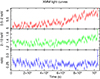 |
Fig. 1. XMM count rate light curves. Top panel: light curve for the energy interval 0.5 − 2 keV. Middle panel: light curve for the energy interval 2 − 10 keV. Bottom panel: ratio between the two energy band. |
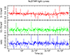 |
Fig. 2. NuSTAR/FPMA background-subtracted count rate light curves. Top panel: light curve for the energy interval 3 − 10 keV. Middle panel: light curve for the energy interval 10 − 79 keV. Bottom panel: ratio between the two energy bands. |
3. Spectral analysis
We performed the spectral analysis using the xspec v12.13.0 package (Arnaud 1996). Fits were performed on the rebinned pn and NuSTAR spectra plus the OM photometric data, using the χ2 minimization technique. All errors are quoted at the 90% confidence level (Δχ2 = 2.71) for one interesting parameter. In all our fits, we included neutral absorption (TBABS model in xspec) from Galactic hydrogen with column density NH = 57.4 × 1020 cm−2 (Kalberla et al. 2005). The cosmological parameters, H0 = 70 km s−1 Mpc−1, ΩΛ = 0.73, and Ωm = 0.27, were adopted.
3.1. The reflection component
We started by investigating the Fe Kα line at 6.4 keV. Initially, we constructed the spectra solely based on a power-law model. Figure 3 illustrates the ratio between the observed data and the model derived from this initial fit. It reveals an amplification in the data/model ratio up to 5 keV, with an emission line at 6.4 keV. To address this issue, we introduced a single Gaussian line with a fixed energy of 6.4 keV and a fixed sigma of zero; in this initial analysis, we focused only on the XMM-Newton/pn spectrum in the 3–10 keV band due to its significantly superior energy resolution compared with NuSTAR. The resulting χ2/d.o.f. was 128/104. Allowing the intrinsic width to vary, we obtained a reduced χ2/d.o.f. of 121/103. Despite the modest enhancement observed, we proceeded with further tests. We modeled the data using two emission lines, both located at 6.4 keV, with one narrow (σ = 0) and one broadened due to relativistic effects (σ free to vary), which led to a significant improvement, with χ2/d.o.f. = 114/102 (Δχ2/Δd.o.f. = −24/−2). The broad emission line had  keV. We concluded that the data were consistent with the presence of both a narrow emission line and a broad emission line.
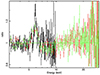 |
Fig. 3. Data/model ratio for the XMM-Newton and NuSTAR spectrum in the 3–30 keV band using the CONST × TBABS × CUTOFFPL model. |
The XMM-Newton/pn and NuSTAR data were then jointly fitted in the 3–30 keV band using a self-consistent reflection model. Given the evidence of both a narrow and a broad component of the Fe Kα emission line, we included two different reflection components. Our model consisted of a power law with an exponential cut-off (Ecutoff), a non-relativistic reflection component (XILLVER García & Kallman 2010; García et al. 2013) and a relativistic one (RELXILL García et al. 2014; Dauser et al. 2016)2. We fixed the source inclination angle at 30°, the outer radius of the accretion disk at 400 Rg and the spin of the black hole to 0.998. This enable us to vary the internal radius of the accretion disk, as the internal disk radius and spin parameter were degenerate. The photon index value in the in RELXILL as in XILLVER was linked to that of the continuum. The ionization parameter in XILLVER was fixed at log ξ = 0, while in RELXILL this was left free to vary. All the other components were free to vary. With this model, we obtained an acceptable fit with χ2/d.o.f. = 338/303 and the following best-fit parameters:  ,
,  , Γh = 1.79 ± 0.02,
  keV and,
  . In Fig. 4, we plot the spectra and the residuals of the model.
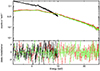 |
Fig. 4. Upper panel: spectroscopic data and best fit model between 3 and 30 keV. Lower panel: residuals of the model. The model used during the fit is CONST × TBABS × (CUTOFFPL + RELXILL + XILLVER). XMM-Newton data are in black, the NuSTAR FMPA data in red, and the NuSTAR FMPB data in green. |
3.2. Soft excess and relativistic reflection
After the analysis of the reflection component, we fitted all XMM-Newton and NuSTAR data in the 0.35–30 keV band. In this model, we were able to better constrain the reflection component and the primary continuum at high energies due to the high NuSTAR sensitivity in the hard X-ray range. The soft excess is clearly visible in Fig. 5, which represents the data in the entire energy range available and the best-fit model discussed in the previous section. We first tested a phenomenological model for the soft excess, namely, a disk blackbody component (DISKBB in XSPEC). We allowed the inner temperature of the disk and the normalization of DISKBB to vary. For the temperature, a best-fit value of 172 ± 7 eV was obtained.
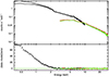 |
Fig. 5. Upper panel: spectroscopic data between 0.35 and 30 keV and the best-fit model. Lower panel: Residuals of the model. The model used during the fit is TBABS × (CUTOFFPL + RELXILL + XILLVER). XMM-Newton data are in black, the NuSTAR FMPA data in red and the NuSTAR FMPB data in green. |
We then tested whether a model including only reflection components is able to explain the soft excess.
We tested two different flavors of XILLVER and RELXILL. In the first case, we used the model CONST × TBABS × (CUTOFFPL + RELXILL + XILLVER) (model A). We employed RELXILL to characterize both the continuum and the ionized reflection originating from the inner disc, which generated a soft excess in this model. Additionally, XILLVER was utilized for the constant reflection component. In RELXILL, the ionization and normalization parameters were kept free, while iron abundance was tied to the value of XILLVER. The outer disk radius was fixed at 400 Rg, while the inner disk radius was left free to vary during the fit. The value of the photon index and that of the cut-off energy in RELXILL – as in XILLVER – were linked to those of the continuum. This model yielded an unacceptable fit with χ2/d.o.f. = 790/369 and strong residuals below 1 keV. We also tried to included a warm absorber, modeled using a CLOUDY table, Ferland et al. (2013) based on a standard, type 1 AGN-illuminating spectrum to model the residuals; however no significant improvement was found (in this case too we obtained a reduced χ2 > 2).
For the second model (model B) we used RELXILLD and XILLVERD, which included the density of the reflecting material as a free parameter (García et al. 2016)3. As free-free absorption is directly proportional to density squared, an uptick in density results in additional thermal emissions from the disk. During the fit, we left the disk density free to vary without imposing a link between the two components. The other parameters were set as in model A. In this case too we found a poor fit, with χ2/d.o.f. = 694/367. For the residuals of the fit see Fig. 6. With this model we found the following best fit parameters for the two densities: ![Mathematical equation: $ \log N [\rm{cm^{-3}}] = 17.69^{+0.01}_{-0.03} $](/articles/aa/full_html/2024/08/aa49524-24/aa49524-24-eq8.gif) and a lower limit at log N[cm−3] of 18.97.
and a lower limit at log N[cm−3] of 18.97.
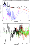 |
Fig. 6. Upper panel: Model B (CUTOFFPL + RELXILLD + XILLVERD) of the X-ray spectrum of HE 1029-1401. The solid thicker black line is the best-fit model, while the dashed lines are the different spectral components: the emission of the hot corona is in red, the non-relativistic reflection component is in blue and the relativistic reflection is in pink. Lower panel: residuals of the model. XMM-Newton data are in black, the NuSTAR FMPA data in red and the NuSTAR FMPB data in green. Model B was used during the fit. |
In the relxillD framework, the maximum density considered was 1019 cm−3. Therefore, we attempted to fit the data using a model incorporating a high-density component to characterize the reflection (REFLIONXHD); this supports densities up to 1022 cm−3. In this model (referred to as model C4), we convolved reflionxHD with kdblur to account for relativistic effects. Instead of xillver, we utilized reflionxhc to describe the reflection, which calculates the reflected spectrum for optically thick material of constant density. Additionally, we introduced a warm absorber (also using a CLOUDY table) in an attempt to better model the soft emission. However, we still obtained a poor fit (χ2/d.o.f. = 683/366), with a density of (7.64 ± 1.22) × 1017 cm−3.
3.3. Testing the two-corona model
In this section, we explain how we studied HE 1029-1401 using the two-corona model. In this model (model D), the soft X-ray spectrum was reproduced only by a thermally Comptonized continuum, modeled using NTHCOMP in xspec. The hard X-ray band was also modeled using NTHCOMP, which parameterized the high-energy rollover using the electron temperature5. To characterize the reflection component, we replaced RELXILL and XILLVER in model D with RELXILLCP and XILLVERCP, respectively. This modification allowed us to fit for the electron temperature instead of using an exponential cut-off. We fixed the inclination angle at 30°, the outer radius of the accretion disk at 400 Rg, and the spin of the black hole at 0.998. During the fit, we assumed that seed photons arose from a multicolor accretion disk; all other parameters were left free to vary.
Using this approach, we obtained an acceptable fit with a χ2/d.o.f. = 429/365. To represent the residuals in the soft band, we included a warm absorber (modeled using the spectral synthesis code CLOUDY, as in the previous section); however, no significant improvement was observed. We then extended our spectral investigation to the optical-UV domain by including the OM data in the fit (model E). Petrucci et al. (2018) applied a model to the archival XMM-Newton/OM and pn data of the source, incorporating two NTHCOMP components (Zdziarski et al. 1996; Życki et al. 1999) to represent the Comptonization continuum originating from the two coronae. Additionally, they included a single non-relativistic reflection component and a component to account for the contribution of the broad-line region (BLR) in the optical/UV band6. As in Petrucci et al. (2018), we considered the potential influence of the BLR on the spectra, including a model for the small blue bump, formed by the Balmer continuum together with Fe II emission. Our approach was based on an additive table with freely adjustable normalization (SMALLBB)7. A comprehensive description of this table for NGC 5548 is provided by Mehdipour et al. (2015). Similar to Petrucci et al. (2018), we accounted for the effect of Galactic extinction by using the REDDEN function in xspec and fixing the reddening during the fit at E(B − V) = 0.0954 as determined by (Güver & Özel 2009)8. The fit resulted in a chi-squared value of χ2/d.o.f. = 437/368. Specifically, the fit indicated that the accretion disk was only minimally ionized ( ), with an internal radius of the accretion disk equal to
  . Furthermore, the photon index and electron temperature were determined to be Γh = 1.86 ± 0.02 and
  =
=  keV for the hot corona and Γw = 2.75 ± 0.05 and
  =
=  keV for the warm corona.
The optical depth of the corona is not one of the fit parameters but may be obtained from the index Γ and the temperature of the electrons, using the equation from Pozdnyakov et al. (1977):
 (1)
(1)
where θe is the electron temperature normalized to the electron rest energy. For the hot and warm corona, we find that τh = 5.4 ± 0.9 and τw = 23 ± 3, respectively.
The fitting parameters are reported in Table 2. Figure 7 shows the spectra and residuals of model E, while Fig. 8 gives the best-fit model. According to this model, the broad-band spectrum of HE 1029-1401 is well described by two Comptonization processes. Specifically, the hard X-ray emission is primarily due to Comptonization in the hot corona, while Comptonization dominates the optical/UV to soft X-ray emission in the warm corona. Possible degeneracy of the hot corona temperature with the reflection fraction was investigated; however, yet no indications of degeneracy were observed (see Fig. 9). The absorption-corrected model luminosity in the 0.001–1000 keV band was 6 × 1045 erg s−1, corresponding to an Eddington ratio of ∼0.1.
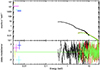 |
Fig. 7. Upper panel: HE 1029-1401 data and its best-fit model. Lower panel: residuals of the model. Model E was used for the fit. XMM-Newton data are in black, the NuSTAR FMPA data in red and the NuSTAR FMPB data in green. |
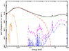 |
Fig. 8. Best-fit model of the UV/X-ray spectrum of HE 1029-1401. The solid thicker black line is the best-fit model while the dashed lines are the different spectral components: the emission of the hot corona is in green, the emission of the warm corona in red, the non-relativistic reflection component is in blue, the relativistic reflection is in pink, and the contribution of the small blue bump is in orange. |
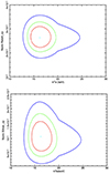 |
Fig. 9. Upper panel: contour plot of RELXILLCP normalization versus the electron temperature in the hot corona. Lower panel: contour plot of XILLVERCP normalization versus electron temperature in the hot corona. The solid blue, green, and red curves represent the 68%, 90%, and 99% confidence levels, respectively. Both plots were generated using model E. |
As a further step in model F, we replaced the warm NTHCOMP component with a table model computed by Petrucci et al. (2020), who performed numerical simulations of the spectra of warm coronae using the radiative transfer code TITAN coupled with the Monte-Carlo code NOAR (Dumont et al. 2003). In its current implementation, this model assumes a blackbody seed photon spectrum, instead of the diskblack body assumed in NTHCOMP9. The free parameters of the TITAN table are the blackbody temperature of the seed photons, the heating power qh in the warm corona, the optical depth τw, and the normalization. During this fit, all the parameters of the TITAN table were left free to vary. The temperature of the seed photons in the NTHCOMP model that describes the hot corona was linked to that of the TITAN table. In this model, we found a chi-squared value of χ2/d.o.f. = 443/368 and the following best-fit parameters for the warm corona: the logarithm of the heating power, log qh (erg s−1 cm−3) was determined to be  ; for the logarithm of Tbb (in units of Kelvin) was 4.38 ± 0.05; the optical depth,
  , and the normalization was
 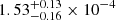 . Given the source distance and luminosity, we can also estimate the radial size of the warm corona from the model. The normalization of the table is directly related to this quantity; using some straightforward calculations (see Petrucci et al. 2020), we obtained ∼ 20 Rg.
Finally in model G, we tested the REXCOR model by Xiang et al. (2022) (see also Ballantyne & Xiang 2020; Ballantyne et al. 2024), which incorporates both warm Comptonization and ionized reflection from a warm corona, illuminated by a lamp-post hot corona. In this model, the accretion energy is distributed between the disk, the warm corona, and the hot corona. The relative strength of the warm Comptonization and of the ionized reflection is driven by the heating fraction of the warm corona and of the hot corona, respectively. The model does not include optical/UV emission; for simplicity, we therefore fitted only the X-ray spectra. Since REXCOR includes blurred ionized reflection, we replaced both the warm Comptonization component and the RELXILL reflection component with REXCOR10. We retained the XILLVERCP component to reproduce distant reflection. In REXCOR, we assumed a lamp-post height of 20 Rg, a black hole spin of 0.99, and an Eddington ratio of 0.1, consistent with the results reported by Ballantyne et al. (2024). We initially found a poor fit in the soft band, with strong residuals near 0.5 keV. To account for these, we included two narrow Gaussian absorption lines, which were found to be at 0.62 keV and 0.74 keV. Gaussian lines of this type, briefly described here, are often needed in this kind of fit (see, for example, Ballantyne et al. 2024). We obtained an acceptable fit with χ2/d.o.f. = 436/364 and the following best-fit parameters for REXCOR: hot corona heating fraction 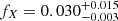 , warm corona heating fraction
  , and optical depth τ < 11 (the lower limit of the model was 10).
4. Discussion and conclusions
The origin of the soft excess in the X-ray spectra of AGN is still debated. Here, we present an analysis of simultaneous XMM-Newton and NuSTAR observation data of the nearby (z = 0.086) AGN HE 1029-1401, with the aim of revealing the nature of the soft excess in this source. Our findings can be summarized as follows:
-
The spectrum of the source shows the presence of a narrow Fe Kα line and a broad (
 keV) Fe Kα line, at 6.4 keV.
 -
To account for emissions resulting from reflection, it was essential to incorporate both a relativistic and a non-relativistic component into the best-fit model.
-
The study confirms the presence of a significant soft X-ray excess below 2 keV. No warm absorber was detected.
-
We observed that the two-corona model describes the source better than the reflection model. Using a phenomenological model, we measured a relatively low temperature of
 =
=  keV, and an optical depth of τh = 5.40 ± 0.85 (assuming a spherical geometry) for the hot corona; for the warm corona, we obtained parameters consistent with lower-luminosity Seyferts, Γw = 2.75 ± 0.05,
  =
=  keV and τw = 23 ± 3.
 -
We also tested two more physical models for the warm corona, namely the TITAN-NOAR table model by Petrucci et al. (2020) and the REXCOR model by Xiang et al. (2022). Despite the different physical assumptions (for a more detailed comparison, see Petrucci et al. 2020), both models provide a good fit to the data. The results are consistent with the presence of a warm corona with an optical depth on the order of 10–20 and with a radial extension of a few tens of gravitational radii.
This is the first NuSTAR observation of the source. Previous X-ray observations of this source were conducted using the XMM-Newton telescope and were analyzed in a previous paper by Petrucci et al. (2018). The results for the warm corona reported in the current study are comparable with those reported in the previous paper, indicating consistency between the two studies. We found slightly different parameters for the hot corona due to a different assumption regarding the temperature of the hot electrons. The results obtained in model G can be compared with the analysis of another observation of the source using the same model, as reported by Ballantyne et al. (2024). We obtained a hot corona heating fraction that is compatible with that of Ballantyne et al. (2024), along with a lower value for the warm corona heating fraction and a slightly larger photon index. We also computed the ratio of the 0.3–10 keV REXCOR and primary continuum fluxes; we obtained a value of 0.36, compatible with that obtained by Ballantyne et al. (2024). Our results are generally consistent with the trends in the REXCOR parameters and the Eddington ratio discussed by Ballantyne et al. (2024), see their Figs. 1–4.
We can compare the results obtained with another quasar for which the two-coronae model was tested: RBS 1055 (Marinucci et al. 2022). In our study, we have observed that the coronae of RBS 1055 are hotter than those found for HE 1029-1401 in this study. This could be due to several factors such as differences in the physical properties of the black hole or the surrounding environment, or variations in the accretion rate and efficiency. Indeed, the Eddington ratio of HE 1029-1401 is a factor two larger than the Eddington ratio of RBS 1055 (Lbol/LEdd ≃ 0.05).
In a broader context, the values obtained from this study are consistent with those known for radio-quiet AGNs as described by the two-corona model (see Petrucci et al. 2018), which are characterized by a warm corona with an optical depth τ ≃ 10 − 40 and an electron temperature KT ≃ 0.1 − 1 keV, and a hot corona that is optically thin (τ ≃ 1) and hot (kT > 20 keV).
In conclusion, the two-corona model provides a good fit for the data, indicating that warm Comptonization is a likely explanation for the soft excess. The broad-band UV/X-ray properties of this luminous quasar are overall consistent with those of local Seyferts, suggesting a similar structure of the accretion flow. This is broadly consistent with the results of Mitchell et al. (2023), who analyzed the spectral energy distribution of a large sample of quasars at z ≤ 2.5 and found that the spectral shape of the optical-UV continuum remains nearly constant across decades of black hole mass for a given luminosity. Mitchell et al. (2023) point out that standard accretion disc models cannot reproduce this behavior, which can instead be explained if the disc is completely covered by a warm Comptonising corona, as long as the UV spectral shape correlates with the accretion rate (which is indeed observed, see Petrucci et al. 2018). In our study, we found that the warm corona had a relatively steep photon index, in agreement with the Eddington ratio measured for HE 1029-1401.
The presence of the warm corona could have significant implications that could directly affect our understanding of the vertical equilibrium of the accretion disk. Models E, F, and G provide a good description of the X-ray spectrum, but their distinct assumptions highlight the necessity for further investigations to enhance our comprehension of warm coronal properties. Future observations of luminous quasars will enable further studies of the soft excess in different accretion regimes.
Data availability
The data analyzed in this paper are publicly available via the XMM-Newton and NuSTAR archives. Readers can refer to Table 1 for the Obs. ID and the details of the observations.
The standard omichain task applies flat-field corrections, detects sources, computes source positions and their count rates, and applies the proper calibration to convert to instrumental magnitudes. HE 1029-1401 is by far the brightest source in the field of view, and its count rates are extracted from a region of 5.3 arcsec.
TBABS×(CUTOFFPL+RELXILL+XILLVER)
Model B: CONST×(CUTOFFPL+RELXILLD+XILLVERD)
Model C: CONST×TBABS×CLOUDY(CUTOFFPL+REFLIONXHC
+KDBLUR×REFLIONXHD)
Model D: CONST×TBABS×(NTHCOMP+NTHCOMP+RELXILLCP+XILLVERCP)
TBABS×REDDEN×MTABLE{CLOUDYTABLE}×(NTHCOMP+NTHCOMP
+ATABLE{SMALLBB}+ATABLE{GALAXY}+XILLVER)
The contribution of the host galaxy is not strong, being a factor of 10 below the nuclear flux in both the optical band (Husemann et al. 2010) and in the UV band, as estimated with GALFIT (K. K. Gupta, private communication). Given the coarse resolution of the OM photometric filters and the fact that most of the filters used here are in the UV band, we chose to include only the BLR emission component, which dominates in the UV band over a contribution from the galaxy (Mehdipour et al. 2015).
Model E: CONST×TBABS×REDDEN×(NTHCOMP+NTHCOMP
+SMALLBB+RELXILLCP+XILLVERCP)
Model F: CONST×TBABS×REDDEN×(NTHCOMP+TITAN
+SMALLBB+RELXILLCP+XILLVERCP)
Model G: TBFEO×CONST(XILLVERCP+REXCOR+NTHCOMP)
Acknowledgments
We thank the referee for useful comments that improved the manuscript. This research was supported by the International Space Science Institute (ISSI) in Bern, through ISSI International Team project #514 (Warm Coronae in AGN: Observational Evidence and Physical Understanding). The research leading to these results has received funding from the European Union’s Horizon 2020 Programme under the AHEAD2020 project (grant agreement n. 871158). This publication was produced while B.V. attending the PhD program in in Space Science and Technology at the University of Trento, Cycle XXXVIII, with the support of a scholarship financed by the Ministerial Decree no. 351 of 9th April 2022, based on the NRRP – funded by the European Union – NextGenerationEU – Mission 4 “Education and Research”, Component 1 “Enhancement of the offer of educational services: from nurseries to universities” – Investment 4.1 “Extension of the number of research doctorates and innovative doctorates for public administration and cultural heritage”. POP acknowledges financial support from the french space agency (CNES) and the High Energy National Programme (PNHE) from CNRS. BV and SB acknowledge financial support from the Italian Ministry for University and Research, through the grants 2022Y2T94C (SEAWIND) and from INAF through LG 2023 BLOSSOM.
References
- Arnaud, K. A. 1996, ASP Conf. Ser., 101, 17 [Google Scholar]
- Ballantyne, D. R., & Xiang, X. 2020, MNRAS, 496, 4255 [NASA ADS] [CrossRef] [Google Scholar]
- Ballantyne, D. R., Sudhakar, V., Fairfax, D., et al. 2024, MNRAS, 530, 1603 [NASA ADS] [CrossRef] [Google Scholar]
- Bianchi, S., Guainazzi, M., Matt, G., Fonseca Bonilla, N., & Ponti, G. 2009, A&A, 495, 421 [NASA ADS] [CrossRef] [EDP Sciences] [Google Scholar]
- Crummy, J., Fabian, A. C., Gallo, L., & Ross, R. R. 2006, MNRAS, 365, 1067 [Google Scholar]
- Dauser, T., García, J., Walton, D. J., et al. 2016, A&A, 590, A76 [NASA ADS] [CrossRef] [EDP Sciences] [Google Scholar]
- Dumont, A. M., Collin, S., Paletou, F., et al. 2003, A&A, 407, 13 [NASA ADS] [CrossRef] [EDP Sciences] [Google Scholar]
- Fabian, A. C., Lohfink, A., Kara, E., et al. 2015, MNRAS, 451, 4375 [Google Scholar]
- Ferland, G. J., Porter, R. L., van Hoof, P. A. M., et al. 2013, Rev. Mex. Astron. Astrofis., 49, 137 [Google Scholar]
- García, J., & Kallman, T. R. 2010, ApJ, 718, 695 [CrossRef] [Google Scholar]
- García, J., Dauser, T., Reynolds, C. S., et al. 2013, ApJ, 768, 146 [Google Scholar]
- García, J., Dauser, T., Lohfink, A., et al. 2014, ApJ, 782, 76 [Google Scholar]
- García, J. A., Fabian, A. C., Kallman, T. R., et al. 2016, MNRAS, 462, 751 [Google Scholar]
- George, I. M., & Fabian, A. C. 1991, MNRAS, 249, 352 [Google Scholar]
- Gliozzi, M., & Williams, J. K. 2020, MNRAS, 491, 532 [Google Scholar]
- Güver, T., & Özel, F. 2009, MNRAS, 400, 2050 [Google Scholar]
- Husemann, B., Sánchez, S. F., Wisotzki, L., et al. 2010, A&A, 519, A115 [NASA ADS] [CrossRef] [EDP Sciences] [Google Scholar]
- Iwasawa, K., Kunieda, H., Awaki, H., & Koyama, K. 1993, PASJ, 45, L7 [Google Scholar]
- Jin, C., Ward, M., Done, C., & Gelbord, J. 2012, MNRAS, 420, 1825 [Google Scholar]
- Kaastra, J. S., & Bleeker, J. A. M. 2016, A&A, 587, A151 [NASA ADS] [CrossRef] [EDP Sciences] [Google Scholar]
- Kalberla, P. M. W., Burton, W. B., Hartmann, D., et al. 2005, A&A, 440, 775 [NASA ADS] [CrossRef] [EDP Sciences] [Google Scholar]
- Magdziarz, P., Blaes, O. M., Zdziarski, A. A., Johnson, W. N., & Smith, D. A. 1998, MNRAS, 301, 179 [NASA ADS] [CrossRef] [Google Scholar]
- Malizia, A., Molina, M., Bassani, L., et al. 2014, ApJ, 782, L25 [NASA ADS] [CrossRef] [Google Scholar]
- Marinucci, A., Vietri, G., Piconcelli, E., et al. 2022, A&A, 666, A169 [NASA ADS] [CrossRef] [EDP Sciences] [Google Scholar]
- Mason, K. O., Breeveld, A., Much, R., et al. 2001, A&A, 365, L36 [NASA ADS] [CrossRef] [EDP Sciences] [Google Scholar]
- Mehdipour, M., Branduardi-Raymont, G., Kaastra, J. S., et al. 2011, A&A, 534, A39 [NASA ADS] [CrossRef] [EDP Sciences] [Google Scholar]
- Mehdipour, M., Kaastra, J. S., Kriss, G. A., et al. 2015, A&A, 575, A22 [NASA ADS] [CrossRef] [EDP Sciences] [Google Scholar]
- Mitchell, J. A. J., Done, C., Ward, M. J., et al. 2023, MNRAS, 524, 1796 [NASA ADS] [CrossRef] [Google Scholar]
- Page, K. L., Schartel, N., Turner, M. J. L., & O’Brien, P. T. 2004, MNRAS, 352, 523 [CrossRef] [Google Scholar]
- Petrucci, P. O., Ursini, F., De Rosa, A., et al. 2018, A&A, 611, A59 [NASA ADS] [CrossRef] [EDP Sciences] [Google Scholar]
- Petrucci, P. O., Gronkiewicz, D., Rozanska, A., et al. 2020, A&A, 634, A85 [NASA ADS] [CrossRef] [EDP Sciences] [Google Scholar]
- Piconcelli, E., Jimenez-Bailón, E., Guainazzi, M., et al. 2004, MNRAS, 351, 161 [Google Scholar]
- Porquet, D., Reeves, J. N., Matt, G., et al. 2018, A&A, 609, A42 [NASA ADS] [CrossRef] [EDP Sciences] [Google Scholar]
- Pozdnyakov, L. A., Sobol, I. M., & Syunyaev, R. A. 1977, Sov. Astron., 21, 708 [NASA ADS] [Google Scholar]
- Ricci, C., Ho, L. C., Fabian, A. C., et al. 2018, MNRAS, 480, 1819 [NASA ADS] [CrossRef] [Google Scholar]
- Ross, R. R., & Fabian, A. C. 1993, MNRAS, 261, 74 [NASA ADS] [CrossRef] [Google Scholar]
- Strüder, L., Briel, U., Dennerl, K., et al. 2001, A&A, 365, L18 [Google Scholar]
- Tortosa, A., Bianchi, S., Marinucci, A., Matt, G., & Petrucci, P. O. 2018, A&A, 614, A37 [NASA ADS] [CrossRef] [EDP Sciences] [Google Scholar]
- Turner, M. J. L., Abbey, A., Arnaud, M., et al. 2001, A&A, 365, L27 [CrossRef] [EDP Sciences] [Google Scholar]
- Walter, R., & Fink, H. H. 1993, A&A, 274, 105 [NASA ADS] [Google Scholar]
- Walton, D. J., Nardini, E., Fabian, A. C., Gallo, L. C., & Reis, R. C. 2013, MNRAS, 428, 2901 [NASA ADS] [CrossRef] [Google Scholar]
- Wisotzki, L., Wamstecker, W., & Reimers, D. L. 1991, A&A, 247, L17 [NASA ADS] [Google Scholar]
- Xiang, X., Ballantyne, D. R., Bianchi, S., et al. 2022, MNRAS, 515, 353 [NASA ADS] [CrossRef] [Google Scholar]
- Zdziarski, A. A., Johnson, W. N., & Magdziarz, P. 1996, MNRAS, 283, 193 [NASA ADS] [CrossRef] [Google Scholar]
- Życki, P. T., Done, C., & Smith, D. A. 1999, MNRAS, 309, 561 [Google Scholar]
All Tables
Obs. ID, start date and exposure time for HE 1029-1401 XMM-Newton and NuSTAR observations.
All Figures
|
Fig. 1. XMM count rate light curves. Top panel: light curve for the energy interval 0.5 − 2 keV. Middle panel: light curve for the energy interval 2 − 10 keV. Bottom panel: ratio between the two energy band. |
| In the text | |
|
Fig. 2. NuSTAR/FPMA background-subtracted count rate light curves. Top panel: light curve for the energy interval 3 − 10 keV. Middle panel: light curve for the energy interval 10 − 79 keV. Bottom panel: ratio between the two energy bands. |
| In the text | |
|
Fig. 3. Data/model ratio for the XMM-Newton and NuSTAR spectrum in the 3–30 keV band using the CONST × TBABS × CUTOFFPL model. |
| In the text | |
|
Fig. 4. Upper panel: spectroscopic data and best fit model between 3 and 30 keV. Lower panel: residuals of the model. The model used during the fit is CONST × TBABS × (CUTOFFPL + RELXILL + XILLVER). XMM-Newton data are in black, the NuSTAR FMPA data in red, and the NuSTAR FMPB data in green. |
| In the text | |
|
Fig. 5. Upper panel: spectroscopic data between 0.35 and 30 keV and the best-fit model. Lower panel: Residuals of the model. The model used during the fit is TBABS × (CUTOFFPL + RELXILL + XILLVER). XMM-Newton data are in black, the NuSTAR FMPA data in red and the NuSTAR FMPB data in green. |
| In the text | |
|
Fig. 6. Upper panel: Model B (CUTOFFPL + RELXILLD + XILLVERD) of the X-ray spectrum of HE 1029-1401. The solid thicker black line is the best-fit model, while the dashed lines are the different spectral components: the emission of the hot corona is in red, the non-relativistic reflection component is in blue and the relativistic reflection is in pink. Lower panel: residuals of the model. XMM-Newton data are in black, the NuSTAR FMPA data in red and the NuSTAR FMPB data in green. Model B was used during the fit. |
| In the text | |
|
Fig. 7. Upper panel: HE 1029-1401 data and its best-fit model. Lower panel: residuals of the model. Model E was used for the fit. XMM-Newton data are in black, the NuSTAR FMPA data in red and the NuSTAR FMPB data in green. |
| In the text | |
|
Fig. 8. Best-fit model of the UV/X-ray spectrum of HE 1029-1401. The solid thicker black line is the best-fit model while the dashed lines are the different spectral components: the emission of the hot corona is in green, the emission of the warm corona in red, the non-relativistic reflection component is in blue, the relativistic reflection is in pink, and the contribution of the small blue bump is in orange. |
| In the text | |
|
Fig. 9. Upper panel: contour plot of RELXILLCP normalization versus the electron temperature in the hot corona. Lower panel: contour plot of XILLVERCP normalization versus electron temperature in the hot corona. The solid blue, green, and red curves represent the 68%, 90%, and 99% confidence levels, respectively. Both plots were generated using model E. |
| In the text | |
Current usage metrics show cumulative count of Article Views (full-text article views including HTML views, PDF and ePub downloads, according to the available data) and Abstracts Views on Vision4Press platform.
Data correspond to usage on the plateform after 2015. The current usage metrics is available 48-96 hours after online publication and is updated daily on week days.
Initial download of the metrics may take a while.