| Issue |
A&A
Volume 665, September 2022
|
|
|---|---|---|
| Article Number | A123 | |
| Number of page(s) | 14 | |
| Section | Cosmology (including clusters of galaxies) | |
| DOI | https://doi.org/10.1051/0004-6361/202243845 | |
| Published online | 16 September 2022 | |
Testing the homogeneity of type Ia Supernovae in near-infrared for accurate distance estimations⋆
1
Institute of Space Sciences (ICE, CSIC), Campus UAB, Carrer de Can Magrans, s/n, 08193 Barcelona, Spain
e-mail: This email address is being protected from spambots. You need JavaScript enabled to view it.
2
Institut d’Estudis Espacials de Catalunya (IEEC), 08034 Barcelona, Spain
3
Department of Physics and Astronomy, Aarhus University, Ny Munkegade 120, 8000 Aarhus C, Denmark
4
Observatories of the Carnegie Institution for Science, 813 Santa Barbara St., Pasadena, CA 91101, USA
5
European Southern Observatory, Alonso de Córdova 3107, Casilla 19, Santiago, Chile
6
Institute for Astronomy, University of Hawai’i, 2680 Woodlawn Drive, Honolulu, HI 96822, USA
7
Department of Physics & Astronomy, University of Oklahoma, Norman, OK 73019, USA
8
Department of Physics & Astronomy, George Washington University, Washington, DC, USA
9
Hamburger Sternwarte, Hamburg, Germany
10
Department of Physics, Florida State University, 77 Chieftan Way, Tallahassee, FL 32306, USA
11
Carnegie Observatories, Las Campanas Observatory, Casilla 601, La Serena, Chile
12
George P. and Cynthia Woods Mitchell Institute for Fundamental Physics and Astronomy, Texas A&M University, Department of Physics and Astronomy, College Station, TX 77843, USA
13
Centre for Space Studies, American Public University System, 111 W. Congress Street, Charles Town, WV 25414, USA
Received:
22
April
2022
Accepted:
9
July
2022
Abstract
Since the discovery of the accelerating expansion of the Universe more than two decades ago, Type Ia Supernovae (SNe Ia) have been extensively used as standardisable candles in the optical. However, SNe Ia have shown to be more homogeneous in the near-infrared (NIR), where the effect of dust extinction is also attenuated. In this work, we explore the possibility of using a low number of NIR observations for accurate distance estimations, given the homogeneity at these wavelengths. We found that one epoch in J and/or H band, plus good gr-band coverage, gives an accurate estimation of peak magnitudes in the J (Jmax) and H (Hmax) bands. The use of a single NIR epoch only introduces an additional scatter of ∼0.05 mag for epochs around the time of B-band peak magnitude (Tmax). We also tested the effect of optical cadence and signal-to-noise ratio (S/N) in the estimation of Tmax and its uncertainty propagation to the NIR peak magnitudes. Both cadence and S/N have a similar contribution, where we constrained the introduced scatter of each to < 0.02 mag in Jmax and < 0.01 in Hmax. However, these effects are expected to be negligible, provided the data quality is comparable to that obtained for observations of nearby SNe (z ≲ 0.1). The effect of S/N in the NIR was tested as well. For SNe Ia at 0.08 < z ≲ 0.1, NIR observations with better S/N than that found in the CSP sample is necessary to constrain the introduced scatter to a minimum (≲0.05 mag). These results provide confidence for our FLOWS project that is aimed at using SNe Ia with public ZTF optical light curves and few NIR epochs to map out the peculiar velocity field of the local Universe. This will allow us to determine the distribution of dark matter in our own supercluster, Laniakea, and to test the standard cosmological model by measuring the growth rate of structures, parameterised by fD, and the Hubble-Lemaître constant, H0.
Key words: supernovae: general / cosmology: observations / distance scale
All of the software developed and used throughout this work is publicly available https://github.com/HOSTFLOWS/flows_sims
© T. E. Müller-Bravo et al. 2022
 Open Access article, published by EDP Sciences, under the terms of the Creative Commons Attribution License (https://creativecommons.org/licenses/by/4.0), which permits unrestricted use, distribution, and reproduction in any medium, provided the original work is properly cited.
This article is published in open access under the Subscribe-to-Open model. This email address is being protected from spambots. You need JavaScript enabled to view it. to support open access publication.
1. Introduction
The expansion rate of the Universe, parameterised by the Hubble-Lemaître parameter, H(z), varies across cosmic time. In the last few years, there has been tremendous effort to measure the local value, known as the Hubble-Lemaître constant (H0), with extremely high precision (< 2% uncertainty; Riess et al. 2021). Recent results have further increased the discrepancy in the value of H0 between the local distance ladder (H0 = 73.04 ± 1.04 km s−1 Mpc−1, baseline with systematics; Riess et al. 2021) and the cosmic microwave background (CMB; H0 = 67.4 ± 0.5 km s−1 Mpc−1; Planck Collaboration VI 2020) measurements, colloquially known as the ‘Hubble tension’, to 5σ (however, see Freedman et al. 2019; Huang et al. 2020; Khetan et al. 2021 for some alternative local measurements). This discrepancy possibly hints towards new physics beyond the standard cosmological model, or alternatively, unaccounted systematic effects (see Di Valentino et al. 2021 for a recent review on the Hubble tension).
In the local Universe, the recession velocities measured from galaxies are affected by a combination of the expansion of the Universe and the gravitational pull of other adjacent galaxies. The measurement of these peculiar velocities is critical for two main reason. First, cosmological analyses with Type Ia Supernovae (SNe Ia) rely on discerning the contribution of peculiar velocities to isolate the cosmological redshift. Secondly, peculiar velocities can be used to inferred the matter-density distribution in the local Universe (Peebles 1976), including our own supercluster, Laniakea (e.g., Tully et al. 2014). The latter provides a direct measurement of the growth-rate of structure, which can be compared to estimates from the early Universe (e.g., Linder 2005).
Current measurements of peculiar velocities often rely on methods such as the Fundamental-Plane and Tully-Fisher relations (e.g., Tully et al. 2016), which provide distances with relatively large uncertainties (with an rms of ∼20 − 30% per galaxy) and only reach out to z ∼ 0.05, standing in the way of the study of the peculiar velocities at further distances. Therefore, there is a lack of higher-precision methods that can also extend to further redshifts for the estimation of distances in the local Universe.
Since the discovery of the accelerating expansion of the Universe more than two decades ago (Riess et al. 1998; Perlmutter et al. 1999), SNe Ia have been extensively used as cosmological distance indicators. In the optical, their light curves can be standardised through empirical relations between their peak brightness, stretch (e.g., Rust 1974; Pskovskii 1977; Phillips 1993), and colour (Tripp 1998). In addition, SNe Ia are brighter in the optical (where detectors are larger as well), compared to other wavelengths, making them easier to observe. Therefore, cosmological analyses with SNe Ia (e.g., Betoule et al. 2014; Scolnic et al. 2018; Abbott et al. 2019) commonly focus on optical wavelengths and rely on light-curve fitters, such as SALT2 (Guy et al. 2005, 2007), for the estimation of their light-curve parameters. Moreover, SNe Ia in the optical have recently been used to estimate the growth-rate of structures (e.g., Boruah et al. 2020; Stahl et al. 2021).
SNe Ia were first proposed as distance indicators in the near-infrared (NIR) around four decades ago (Elias et al. 1981, 1985, but also see Meikle 2000), where they seem to be true ‘standard candles’ (as opposed to ‘standardisable candles’ in the optical). In other words, an estimation of the NIR peak magnitudes is all that is needed to measure distances. The NIR light curves of SNe Ia present lower intrinsic dispersion than the optical light curves and have the advantage of being less affected by dust extinction, which makes them exceptional for measuring cosmological distances (e.g., Krisciunas et al. 2004; Wood-Vasey et al. 2008; Freedman et al. 2009; Barone-Nugent et al. 2012; Phillips 2012; Weyant et al. 2014; Friedman et al. 2015; Johansson et al. 2021). Moreover, the NIR light curves of SNe Ia have already been used to constrain H0 to a few percent (e.g., Burns et al. 2018; Dhawan et al. 2018).
The low intrinsic dispersion of SNe Ia in the NIR raises the possibility of using them to achieve accurate cosmography by measuring peculiar velocities of local galaxies, reaching out to z ∼ 0.1 or even beyond. However, the sample of SNe Ia observed in the NIR is currently low due to several factors: low NIR detector sensitivity in the past; SNe Ia are fainter at these wavelengths, where the sky brightness dramatically decreases the contrast for the (SN) observations, thus needing to integrate for longer; and the number of facilities with NIR instruments (compared to optical ones) is low. However, by taking advantage of the exceptional homogeneity of the SNe Ia in the NIR, we can possibly reconstruct their light curves with just a few photometric data points (e.g., Krisciunas et al. 2004), increasing the total number of observed objects.
Given the large stream of optical photometry publicly provided by the Zwicky Transient Facility (ZTF; Graham et al. 2019), which works as a precursor and testing ground for LSST, hundreds to thousands of SNe Ia are being followed-up with high-cadence (average of 2 days) gr-bands photometry1. Thus, ZTF can provide the optical data coverage while NIR photometry can be obtained with other facilities. This work aims to test how accurately we can retrieve NIR peak magnitudes with well-covered optical light curves and few NIR epochs for distance estimations. Our results will give assurance to use SNe Ia with public ZTF gr-band light curves with sparse data in the NIR to reconstruct the cosmography of our local supercluster, measure the growth-rate of structure and H0, and test ΛCDM and alternative cosmological models. In the future, this can be extended to use optical data from the Rubin Observatory Legacy Survey of Space and Time (LSST) and NIR data from telescopes such as the Roman Space Telescope and James Webb Space Telescope.
This paper is organised as follows: in Sect. 2, we present the sample of SNe Ia and the quality cuts used throughout this work, together with the SNooPy fits. In Sect. 3, we describe the simulations of NIR light curves. The comparison between the fits of the simulations and our reference sample is presented in Sect. 4, while the study of systematics is presented in Sect. 5. In Sect. 6, we estimate distances using the reference sample of SNe Ia and compare them with those from the simulations. Finally, we summarise and conclude in Sect. 7. The scripts used throughout this work can be found online2.
2. Data and method
In this work, we use the Carnegie Supernova Project (CSP; Hamuy et al. 2006) sample as it is one of the most comprehensive samples of SNe Ia with extensive uBgVriYJH (optical to NIR) coverage and well-understood magnitude systems to date. The data from CSP-I consists of three data releases (DRs) described in Contreras et al. (2010, DR1), Stritzinger et al. (2011, DR2) and Krisciunas et al. (2017, DR3), while the data from CSP-II are described in Phillips et al. (2019) and Hsiao et al. (2019). CSP-II does not have a public DR to date, but one is in progress (Suntzeff et al., in prep.). We include all the 134 SNe Ia from CSP-I and 202 from CSP-II (the cosmology sub-sample from Phillips et al. 2019). Thus, the CSP sample we use consists of a total of 336 SNe Ia.
As CSP observations have used different filters and telescopes throughout the different campaigns, we apply S-corrections (Stritzinger et al. 2011) to work in a single magnitude system, simplifying the handling of data. This is specifically useful for those CSP-I SNe with multiple V, Y, or J bands, and for combining SNe from CSP-I and CSP-II.
2.1. Light-curve fitter
Currently, a small number of SNe Ia light-curve fitters work in the NIR, such as SNooPy (Burns et al. 2011), PISCOLA (Müller-Bravo et al. 2022), and BayeSN (Mandel et al. 2022). The difference between them is that SNooPy and BayeSN are template-based fitters (i.e. trained on well-sampled SNe Ia) while PISCOLA uses a data-driven approach that relies on Gaussian processes (GPs; Rasmussen & Williams 2006). However, for the aim of this work, as we need to reconstruct the NIR light curves with a few photometric points, PISCOLA is not an option. On the other hand, the difference between SNooPy and BayeSN is that the latter uses a probabilistic approach, constructing a hierarchical Bayesian model for the spectral energy distribution of SNe Ia, therefore obviating the need of ad-hoc K-corrections (as is the case of SNooPy). However, BayeSN assumes a dust extinction law for SNe Ia, so it does not have the same freedom as SNooPy. Additionally, BayeSN is not public, so we choose to use SNooPy, with its latest version (v2.6), trained on the updated NIR spectral templates from Hsiao et al. (2007). However, SNooPy, as in the case of other light-curve fitters, heavily relies on optical data for accurate fitting.
To fit the SNe Ia, we use SNooPy with the max_model model, as we require measurements of Jmax and Hmax. The resulting fits provide the following output parameters: Tmax, sBV, and xmax, where Tmax is the time of B-band peak magnitude, sBV is the ‘colour stretch’ parameter as defined in Burns et al. (2014)3 and xmax represents the peak magnitude in x-band, for each of the observed filters. An example fit for SN 2004eo is shown in Fig. 1. We note that the multi-colour light-curve templates (optical to NIR) are driven by the values of Tmax and sBV. For more information on why the max_model model is used instead of other models, such as EBV_model2, see Appendix A. All magnitudes presented are in the CSP natural system and the reported uncertainties from SNooPy fits are statistical uncertainties only.
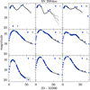 |
Fig. 1. SNooPy fit of the multi-colour (uBgVriYJH) light curves of SN 2004eo. The max_model model is used throughout this work. |
2.2. Sample cuts
As not all CSP SNe are useful for the purpose of this work, we proceeded to apply some cuts to the initial sample. We only used SNe Ia labelled as ‘normal’ according to Krisciunas et al. (2017) and Ashall et al. (2020). A current re-analysis of SNe Ia performed by Phillips et al. (in prep.) has re-labelled 1991T-like SNe from the CSP sample. Thus, we use their definition henceforth. This cut removes 34 of the initial 336 SNe Ia: one 2003fg-like SN, four 1986G-like SNe, 10 1991T-like SNe, sixteen 1991bg-like SNe, and 3 peculiar SNe (labelled as ‘...’ in Krisciunas et al. 2017).
We then proceed to remove any SN without g, r, J, or H bands, as these are strictly required for our analysis: g and r being the bands used by ZTF while J and H being the NIR bands commonly available. The Y band is not included as catalogues of standard stars for this band are not available for the whole sky, which are needed for the calibration. We note that 80 SNe do not have a g band (all from CSP-II), while all of them have an r band. In this step, we identified and removed 138 of the remaining 302 SNe.
The next cut requires the SN to have coverage of the optical peak as the estimation of Tmax is fundamental when fitting the light curves of SNe Ia (Sects. 2.3 and 3). For this, we need to have one or more photometric points at least two days before and two days after Tmax in B, g, V, or r bands, providing an accurate estimation of the location of the peak. Almost all the SNe have the optical decline well covered, while some do not have pre-peak observations. We note that the SNe are fitted with SNooPy first to estimate Tmax. This cut removes 53 of the remaining 164 SNe.
Finally, we require at least one photometric point before and after the time of J-band peak (Jmax) and H-band peak (Hmax), as precise measurements of Jmax and Hmax are needed. These constraints are less stringent compared to those in the optical as the light-curve fits are mainly driven by the optical bands. In addition, we require at least three photometric points, in each NIR band, to have a relatively good coverage of the light-curve peak. We note that the SNe are fitted with SNooPy first, with the same model as before, to estimate the locations of the NIR peaks. Here, we remove 61 of the 111 remaining SNe, leaving us with a sample of 50 CSP SNe Ia, comprising our reference sample.
In the top panel of Fig. 2, we show the redshift distribution of the reference sample and the complete CSP-I + CSP-II sample. One downside of the cuts applied is that all objects with z ≳ 0.05 are removed. An object at z = 0.1 is approximately 1.5 mag fainter than one at z = 0.05, which translates into a poorer signal-to-noise ratio (S/N) of the observations, making the estimations of light-curve parameters less accurate. However, SNe at higher z also have faster restframe cadences compared to those at lower z (for the same observed cadence), although at z ≲ 0.1, there is only a small difference. The effects of cadence and S/N are later discussed in Sects. 5.1–5.3.
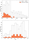 |
Fig. 2. Comparison between the reference and the entire CSP samples. Top panel: redshift distribution of CSP-I + CSP-II (empty bars) and the 50 SNe Ia comprising our reference sample (orange bars). Bottom panel: sBV distribution of SNe Ia from CSP-I + CSP-II (empty bars) labelled as ‘normal’ and the reference sample (orange bars). The values of sBV were obtained by fitting the SNe with SNooPy using the max_model model. Only the ‘normal’ SNe are shown in this case as SNooPy mainly provides templates for these objects and not other types. |
In the bottom panel of Fig. 2, we show the sBV distribution of the reference sample and the ‘normal’ SNe Ia from the CSP-I + CSP-II sample. Both distributions span approximately the same range in sBV, with no major differences apart from the number of objects.
The cuts from this section are summarised in Table 1, where the numbers are also split by survey (CSP-I and CSP-II). Tighter constraints could be used, although this would further reduce the size of our sample, reducing statistics as well, and change the distribution of light-curve parameters.
2.3. Reference Sample
Although the data quality of CSP-I and CSP-II are almost identical, the data coverage in the NIR bands is not the same. The NIR light curves of SNe Ia from CSP-I are on average better populated than those from CSP-II. Examples of SNe from both surveys are shown in Figs. 3 and 4. This sample of 50 SNe Ia are later used as reference for the simulations in Sect. 3.
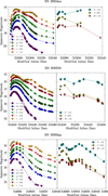 |
Fig. 3. Multi-colour light curves of SNe 2004eo (top), 2005M (middle), and 2009aa (bottom) from CSP-I. |
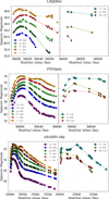 |
Fig. 4. Multi-colour light curves of SNe LSQ12bld (top), PTF13ebh (middle; Hsiao et al. 2015), and ASASSN-14lp (bottom; Shappee et al. 2016) from CSP-II. |
We create three different sets of reference values according to the bands used for the fits: (i) all bands; (ii) grJH; and (iii) gr (see Table 2). We note that sets (ii) and (iii) are mainly used as control sets to test whether there are any discrepancies in the output parameters (e.g., Tmax) compared to using all bands (see Sect. 4).
3. Simulations
Given that we want to replicate what real observations would be (i.e. optical bands well covered with few NIR data points), the simulations consist of taking the complete gr-band light curves, plus n epochs of coeval J- and H-band photometric points, for n = 1, 2, and 3. We note that we are sampling from the available photometry (henceforth referred to as ‘simulations’ in this paper). Combinations without repetition of the JH-band photometry are used for this:
 (1)
(1)
where C is the total number of combinations and N is the total amount of J/H epochs, for each band individually. For instance, a SN with 10 epochs of coeval J- and H-band photometric points would have C1(10) = 10, C2(10) = 45 and C3(10) = 120 simulations for 1, 2, and 3 J/H epochs, respectively.
The resulting simulations are then fit, using SNooPy, as described in Sect. 2.3, and the output parameters saved for a later comparison (Sect. 4). In Fig. 5, we show an example of simulations with n = 1 for ASASSN-14hu, with the respective fits for each simulation in J and H bands. As can be seen from the fits, the values of Jmax and Hmax highly depend on the epochs of the photometry. We note that as we are dealing with few J and H photometric epochs, a proper estimation of the NIR peaks is, in principle, not possible, so we measure the time with respect to Tmax, which can be accurately obtained from the complete optical gr-band light curves.
 |
Fig. 5. Fits of single-epoch JH simulations for ASASSN-14hu. Each colour represents a different simulation and fit for the NIR photometry of the SN. |
We also performed simulations for J and H bands separately to test whether having only one NIR band produces similar results compared to having two. To summarise, we carried out simulations with grJ, grH, and grJH bands (see Table 2), each with 1, 2, and 3 NIR epochs. The different sets of fits for the reference sample and simulations are summarised in Table 2.
4. Analysis
Assuming that SNe Ia are standard candles in the NIR, peak NIR magnitudes can be directly used to estimate distances without further corrections (e.g., from stretch or colour). Thus, our main interest is to see how well we can measure Jmax and Hmax using just a few NIR photometric points. However, as can be seen in Fig. 5, the retrieved peak magnitudes highly depend on the time of the observations with respect to Tmax. We therefore define three different metrics to understand what type of observations are best at obtaining accurate Jmax and Hmax measurements:(i) time of the closest J/H epoch with respect to Tmax; (ii) mean time of the J/H epochs with respect to Tmax; and (iii) difference between the earliest and latest (i.e. range) J/H epochs. Note that in the case of the simulations with only one epoch (n = 1), metrics (i) and (ii) are the same, while (iii) is not calculated. Also note that these metrics are defined in the restframe, i.e. epochs are corrected for time dilation using the SN redshift.
In Fig. 6, we show Jmax and Hmax residuals between the simulations and the reference sample (using all bands) as a function of metric (i), for simulations with grJH bands and n = 1. From this comparison, we see that the scatter in the residuals tends to be smaller around Tmax, with the smallest scatter before Tmax, and increases at later epochs. In general, the scatter is smaller for the H band compared to the J band. This is consistent with what has been found in other works (e.g., Dhawan et al. 2015). Additionally, we note that offsets in Jmax and Hmax tend to be larger where the NIR light-curve templates have a larger gradient or slope (see Fig. 5 and Sect. 5 for further discussion). The weighted mean and the uncertainty on the weighted mean of these residuals are summarised in Table 3. Given that the uncertainties in light-curve parameters from the reference sample and simulations are correlated (both use the same photometry), henceforth, we only use those from the latter for the statistics.
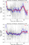 |
Fig. 6. Jmax (top panel) and Hmax (bottom panel) residuals, between simulations with coeval coeval J- and H-band epoch and reference value. The weighted mean and uncertainty on the weighted mean in bins of two days are shown in blue. A “correction snake” and its uncertainty are calculated by fitting the residuals with GPs (red line and shaded region), while N is the total number of simulations. |
As we are aiming to reduce the scatter, ideally, we would need data around Tmax. Unfortunately, as it is hard to obtain photometric data at specific epochs due to different constraints (weather, time, allocation, etc.), we have to look for a time window with a large-enough range. We noticed that a time range between −5 to 15 days with respect to Tmax possess a relatively low scatter in Jmax and Hmax. The weighted mean (Δ) and weighted standard deviation (σ) of the residuals in this time window are Δ = 0.004 mag and σ = 0.047 mag, and Δ = −0.006 mag and σ = 0.053 mag, for Jmax and Hmax, respectively.
In the case of the simulations with grJ or grH bands, similar results are obtained, meaning that a single NIR band is as good as two NIR bands (see Fig. B.1). When comparing with the simulations with n = 2 and n = 3, the scatter in the residuals is reduced. For n = 2, we find a scatter in Jmax of 0.039 mag, while for n = 3, we find 0.030 mag. In the case of Hmax, the scatter gets reduced to 0.043 mag and 0.038 mag, for n = 2 and n = 3, respectively. Although the offsets change for n = 2, 3, they still remain relatively small (≲0.01 mag). We also found that metrics (ii) and (iii) are not as relevant as metric (i) (see Fig. 7 for simulations with n = 3). In other words, the most important point is to have a NIR photometric epoch close to Tmax. Having more photometric points helps reducing the scatter, although they are less essential for an accurate estimation of Jmax or Hmax.
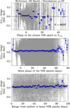 |
Fig. 7. Jmax residuals between simulations with three coeval J- and H-band epochs and reference sample as a function of metrics (i), (ii), and (iii) (top, middle, and bottom panels, respectively). The weighted mean and uncertainty on the weighted mean in bins of two days are shown in blue for each of the panels. The residuals in Jmax do not vary much as a function of metrics (ii) and (iii), which means that metric (i) is the most relevant for estimating Jmax. The metrics are described in Sect. 4, while N is the total number of simulations. The global offsets in the middle and bottom panels are driven by those simulations with phases ≲ − 5 days and ≳30 days from the top panel. |
When comparing other light-curve parameters, such as gmax, rmax, sBV, and Tmax, between the reference sample and simulations, we found negligible differences (≲0.02 mag) for the first three parameters and < 0.1 day for the last. These very small differences are produced by the NIR data. Although the fits are mainly driven by the optical light curves, the NIR also affects the estimation of Tmax, and therefore, the other light-curve parameters. When using grJH bands and gr bands as reference, we found similar results as when using all bands as reference (we note that for gr bands only, Jmax and Hmax cannot be calculated).
5. Data-quality systematics
As was previously mentioned, the light-curve fits heavily rely on having a proper estimation of Tmax. Any uncertainty in this parameter is propagated to others, such as the NIR peak magnitude. It follows that having small uncertainties and fast cadence is ideal, particularly in the optical bands. However, this is not always possible. In this section, we test how cadence and S/N affect the estimations of Jmax and Hmax.
5.1. Cadence
To measure the effect of cadence, we started by taking the gr-band light curves of the reference sample and simulated different cadences by taking every two observations in each light curve, every three, every four, and so on. We make sure to ‘move’ the first observation taken so we have different starting points until all epochs before Tmax have been used (the reader should not confuse these simulations with those from Sect. 3). We note that the observer-frame cadences across the optical filters are very similar for a single SN as CSP observations were taken with multiple filters during the same nights (see Figs. 3 and 4). Our reference sample has an average cadence of ∼3.1 days in gr, while the simulations have cadences > 3.1 days.
In the top panel of Fig. 8, we show the difference in Tmax between the cadence simulations and reference sample (ΔTmax). For the cadence simulations, only gr-bands are used and all those with restframe cadences < 10 days are considered. Surprisingly, we can see that despite the inclusion of simulations with slow cadences (i.e. large gaps of up to ten days), the distribution of ΔTmax has a standard deviation of ∼0.5 days, with a weighted average of 0.01 days (weighted by the uncertainty in Tmax of the simulations). By looking at the significance (ΔTmax/σTmax; bottom panel of Fig. 8), we see that most are relatively small, with an average of 0.13, while very few simulations have a significance greater than 3.0.
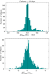 |
Fig. 8. Tmax comparison for cadence simulations. Top panel: difference in Tmax between the cadence simulations (Sect. 5.1) and reference sample (ΔTmax). All simulations with restframe cadences < 10 days are considered here. The weighted average Δmax is 0.01 days (vertical dotted line). Bottom panel: ΔTmax over the uncertainty in Tmax (i.e. significance) for the cadence simulations. The average significance is 0.13 (vertical dotted line), while very few simulations have a significance greater than 3.0. The average uncertainty in Tmax (0.19 days) is much larger than the weighted average ΔTmax. |
This accurate estimation of Tmax can be explained by having small uncertainties and a good coverage across the light curves, that is, having at least one observation before and after peak, as this helps anchor the light-curve templates. Looking at Fig. 9, we see how the weighted average and standard deviation of ΔTmax depend on cadence, shown as red squares with error bars. All weighted means are < 0.1 days. For cadences < 7 days, the standard deviations are all < 0.3 days, while for cadences > 7 days, they are > 0.5 days, but less than 1 day. We note that average observer-frame cadences of ZTF (2 days) and LSST (assuming 3-days baseline cadence in each band) would have a very small effect on the estimation of Tmax, while some additional scatter in Tmax is expected for cadences such as that of DES (7 days; Brout et al. 2019). We also note that the difference between observer-framer and restframe cadences is less than one day at z < 0.1.
 |
Fig. 9. Difference in Tmax between the cadence simulations (Sect. 5.1) and reference sample (ΔTmax) as a function of restframe cadence. The binned average and standard deviation of ΔTmax are shown as red squares with error bars. The average observed cadences for ZTF (2 days), LSST (assuming 3-day baseline cadence per filter), CSP (3.1 days for the reference sample), and DES (7 days; Brout et al. 2019) are shown as vertical dotted lines. We note that the restframe cadence is faster by a factor of 1 + z than the observed cadence; N is the total number of simulations. |
We further test how any uncertainty in Tmax could propagate to Jmax and Hmax by multiplying ΔTmax with the gradient (slope) of the NIR light-curve templates (using the definition of error propagation), resulting in additional scatter. We note that the shape of the templates depends on the value of sBV, which is obtained from the fits of the gr-band light curves from the reference sample. The results are shown in Fig. 10. The average offset is negligible and the scatter is < 0.02 mag in J band for NIR observations between −10 and 50 days. The scatter is much smaller for H band (< 0.01 mag) than for J band, as the former has a smoother light-curve shape with smaller gradient (see Fig. 5). We note that these scatters are even lower around Tmax and can be considered as upper limits as cadences of up to 10 days are being considered here. We also note that these values are much smaller than the scatter found in Sect. 4 (i.e. ∼0.05 mag), although these have to be added in quadrature.
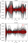 |
Fig. 10. Effect that restframe cadence (up to 10 days) in the optical gr-bands has on the estimation of the NIR peak magnitudes. The grey lines represent ΔTmax multiplied by the gradient of the NIR light-curve template bands as a function of phase, for each simulated SN from Sect. 5.1. We note that the shape of the templates depends on the value of sBV, which is obtained from the fits of the gr-band light curves. The average NIR peak magnitude offset is shown as a red line for J (top panel) and H (bottom panel) bands. The 1σ scatter in NIR peak magnitude (red shaded region) is < 0.02 mag in J band and much smaller for H band (< 0.01 mag). |
Apart from the scatter introduced by different cadences, we can isolate the effect of coverage of the rise of the light curves, which also affects the estimations of Tmax. In Fig. 11, we show the difference in Tmax between the cadence simulations and reference sample (ΔTmax) as a function of the phase of the first observation used for the simulations. One can see that independent of the cadence of the simulations, the scatter in ΔTmax starts rapidly increasing for the first observations with phases of ≳ − 5 days. This is really important as it suggests that real observations should ideally cover earlier epochs (< − 5 days) in gr-bands to provide precise estimations of Tmax. However, observations starting at later epochs can still be used, with the caveat of introducing additional scatter.
 |
Fig. 11. Difference in Tmax between the cadence simulations (Sect. 5.1) and reference sample (ΔTmax) as a function of the phase of the first observation. The simulations are split in three groups according to the cadence (cad) range: 2 < cad < 5 days (purple crosses), 5 < cad < 8 days (pink circles), and 8 < cad < 10 days (gold squares). Tmax is shown as a vertical dashed line. Independent of the cadence, the scatter in ΔTmax starts rapidly increasing for the first observations with phases of ≳ − 5 days. |
5.2. Signal-to-noise in the optical
The effect of S/N is important as it does not only depend on things such as the detector, length of the exposures, and so on, but also on the distance and brightness of the objects. To measure how the S/N of optical observations affects the estimation of Tmax, a similar procedure is followed as before. We started by taking gr-band light curves of the reference sample and simulated different S/N by multiplying the flux uncertainties in each of the light curves by x, for x = 2, 3, 4, 5, 6, 7, and randomly sampling new observations using a normal distribution with the new uncertainties. We note that the uncertainties in the CSP observations are relatively small in part due to observing nearby SNe. We use the S/N in g band as reference, although the S/N in r band is very similar. For each SN, the median S/N is used instead of the mean as the S/N greatly changes as a function of light-curve phase.
After calculating the difference in Tmax between the S/N simulations and reference sample, we find relatively similar results compared to those in Sect. 5.1. The distribution of ΔTmax has a standard deviation of 0.13 days, with a weighted average of 0.02 days (top panel of Fig. 12), while the average significance in ΔTmax is 0.23 with almost no simulations with a significance greater than 3.0 (bottom panel of Fig. 12).
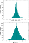 |
Fig. 12. Tmax comparison for S/N simulations. Top panel: difference in Tmax between the S/N simulations (Sect. 5.2) and reference sample (ΔTmax). The weighted average ΔTmax is −0.007 days (vertical dotted line). Bottom panel: ΔTmax over the uncertainty in Tmax (i.e. significance) for the S/N simulations. The average significance is 0.23 (vertical dotted line), while very few simulations have a significance greater than 3.0. The average uncertainty in Tmax (0.12 days) is larger than the weighted average ΔTmax. |
Figure 13 shows ΔTmax as a function of S/N. This figure shows that the scatter in ΔTmax slowly increases as the S/N decreases (note the logarithmic scale in the x-axis). Despite the decrease in S/N of the simulations, SNooPy is still able to retrieve a relatively accurate estimation of Tmax. This can be explained by having decent coverage throughout the entire light curves.
 |
Fig. 13. Difference in Tmax between the S/N simulations (Sect. 5.2) and reference sample as a function of S/N. The binned weighted mean and standard deviation of ΔTmax are shown as red squares with error bars; N is the total number of simulations. |
We also test how the uncertainty in Tmax propagates to Jmax and Hmax. The results are shown in Fig. 14. Although Jmax seems to have some slight offset, this is very small (< 0.005 mag). The effect of S/N only introduces an additional scatter ≲0.02 mag in the J band and < 0.01 mag in the H band, being even lower around Tmax (smaller than the scatter found in Sect. 4). These are similar to the dispersion found in Sect. 5.1. As we are including simulations with S/N as low as ∼10, these dispersions can also be considered as upper limits. Observations of low-z SNe Ia, such as those observed by the CSP, typically have small photometric uncertainties due to their intrinsically bright nature.
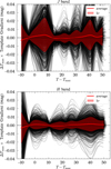 |
Fig. 14. Effect that S/N in the optical gr-bands has on the estimation of the NIR peak magnitudes. The grey lines represent ΔTmax multiplied by the gradient of the NIR light-curve template bands as a function of phase, for each simulated SN from Sect. 5.2. We note that the shape of the templates depends on the value of sBV, which is obtained from the fits of the gr-band light curves. The average NIR peak magnitude offset is shown as a red line for J (top panel) and H (bottom panel) bands. The 1σ scatter in NIR peak magnitude (red shaded region) is ≲0.02 mag for J band and < 0.01 mag for H band. |
From this set of tests, we conclude that SNooPy can give an accurate estimation of Tmax, and therefore, Jmax and Hmax, for different cadences and S/N in gr-bands. Additionally, H band is less affected by uncertainties in the estimation of Tmax, compared to J band, due the smooth and relatively flat shape of the SN light curve at these wavelengths.
5.3. Signal-to-noise in the NIR
The effect of S/N is also important for NIR observations of SNe Ia, especially as the S/N is lower at these wavelengths compared to the optical. To test the effect of S/N of NIR observations in the estimation of the NIR peaks, we proceed in a similar fashion as described in the previous section. However, this time the complete gr-band light curves are used together with the closest NIR epoch to Tmax. The uncertainty in the NIR photometric point is then varied to simulate different S/N and the light curves are fitted to estimate Jmax and Hmax.
The average S/N of our reference sample is 54 and 39 in J and H bands, respectively. These are relatively low compared to the average S/N of ∼100 in g band and SNe Ia at higher redshift would have even lower values. The CSP sample contains thirteen SNe Ia with J-band data at z > 0.08 with an average S/N of ∼21 and only eight objects with H-band data with an average S/N of ∼8. There is not only a large difference in S/N between low-z (≲0.05) and high-z SNe (≳0.08), but also between NIR bands.
Figure 15 shows the residual in Jmax between NIR S/N simulations with J-band S/N > 21 and the reference sample (ΔJmax). The weighted mean and standard deviations of ΔJmax are 0.006 mag and 0.070 mag, respectively. The scatter is larger than the one found in Sect. 4 (∼0.05 mag), which was expected. The weighted mean and standard deviations of ΔHmax are 0.014 mag and 0.107 mag, respectively, for simulations with S/N > 8. These are much larger compared to the J band and is due to the lower S/N.
 |
Fig. 15. Residual in Jmax between NIR S/N simulations with J-band S/N > 21 (Sect. 5.3) and the reference sample (ΔJmax). The weighted mean and standard deviations are 0.006 mag and 0.070 mag, respectively. |
In Fig. 16, we show the ΔJmax (top panel) and ΔHmax (bottom panel) as a function of S/N. The scatter in both bands is similar for the same S/N, although the average S/N is lower in the H band. This test shows the importance of having high S/N observations in the NIR. If the aim is having an accurate estimation of Jmax and Hmax for SNe Ia at z ∼ 0.1, NIR observations with better S/N than those obtained by CSP must be achieved (see Fig. 16). We note that, however, several of the CSP observations were obtained with a 1 meter telescope (Swope), so using 2 meter-class telescopes or better is ideal. We also note that in the restframe, the J-band light curves of SNe Ia are intrinsically brighter than their H-band light curves, making J-band observations better suited for measuring distances at high z.
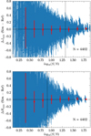 |
Fig. 16. Difference in Jmax (top panel) and Hmax (bottom panel) between the NIR S/N simulations (Sect. 5.3) and reference sample as a function of S/N. The binned median and standard deviations are shown as red squares with error bars. Simulations with all S/N values are shown in here. The average S/N of CSP SNe Ia at z > 0.08 are shown as vertical lines (21 and 8 for J and H bands, respectively); N is the total number of simulations. |
6. Near-infrared distances
The final step in this work is to calculate the precision in the distance estimations from the simulations of Sect. 4. Assuming that SNe Ia are standard candles in the NIR, the peak apparent magnitude is the only parameter necessary to calculate distances and its uncertainty is directly propagated to the measured distance:
 (2)
(2)
where μ is the distance modulus, mmax is the peak apparent magnitude in a NIR band (e.g., Jmax or Hmax) and M is the peak absolute magnitude in that same band. To calculate distances, a cosmological model needs to be fitted. For simplicity, we assume a flat ΛCDM cosmology and fix the value of M (MJ = MH = −18.5 mag), fitting only H0 and the intrinsic dispersion of SNe Ia (σint). Only SNe at z > 0.01 are used as the contribution from peculiar velocities is relatively small at these redshifts. This reduces our reference sample to 36 objects. The resulting Hubble diagram in J band is shown in Fig. 17 (red circles). The Hubble residuals have an rms of 0.166 mag, while σint = 0.14 mag was obtained.
 |
Fig. 17. Hubble diagram in J band. Only SNe Ia with z > 0.01 were used as the contribution from peculiar velocities is relatively small at these redshifts. The reference sample was used to fit H0 and the intrinsic dispersion (σint), keeping the peak absolute magnitude in J band (MJ = −18.5 mag) fixed. The rms for the reference sample (red) and the simulations with n = 1 (grey) are 0.166 mag and 0.180 mag, respectively. |
To calculated distances with the simulations, we use the values of H0 and σint obtained with the reference sample and apply the offsets found in Sect. 4:
![Mathematical equation: $$ \begin{aligned} \mu = [m_{\rm max} + \Delta (b, n, p)] - M, \end{aligned} $$](/articles/aa/full_html/2022/09/aa43845-22/aa43845-22-eq3.gif) (3)
(3)
where the offset Δ(b, n, p) depends on the NIR band (b), the number of epochs (n), and the phase (p) of the epoch closest to Tmax. The uncertainty associated to this offset is added in quadrature. If one assumes that SNe Ia are standard candles in the NIR, one would expect to measure the same offsets, as found in Sect. 4, in Jmax and Hmax for a different sample of SNe Ia. Therefore, these can be used as a correction term.
The J-band Hubble diagram for simulations with n = 1 is shown in Fig. 17 (grey circles). Using the simulations with phase between −5 days and 15 days, where a low scatter in Jmax was found (see Sect. 4), an rms of 0.180 mag is obtained. Although the simulations have larger scatter than the reference sample, the difference is relatively small (0.014 mag).
In the case of the H band, the reference sample and the simulations have Hubble residuals rms of 0.149 mag and 0.147 mag, respectively. The rms values are very similar, being slightly smaller for the simulations (a negligible difference of 0.002 mag). Although a larger scatter was expected for the simulations, we note that sample used to build the Hubble diagram is not exactly the same as that used in Sect. 4. If the offsets found in Sect. 4 are not applied, very similar results are found, only increasing the rms in ∼0.002 mag for J and H bands. Therefore, we believe that these offsets might not be necessary to apply.
As expected, the scatter in H band is lower than in the J band. In addition, for the H band σint = 0.12 mag, smaller than for the J band. If the simulations are used to fit H0 and σint instead of the reference sample, we find the same rms values. The values of H0 and σint do change, but the differences are insignificant (≲1.5σ) for both the J and H bands.
By using simulations with 2 and 3 NIR epochs, the scatter is reduced to 0.178 mag and 0.168 mag for the J band and 0.138 mag and 0.127 mag for the H band, respectively. Although the reduced scatter is expected, we did not expect to have lower scatter for the simulation than for the reference sample in the H band. This could be caused by limitations in our analysis. For instance, SNooPy was trained on a sub-sample of the SNe Ia from CSP, which can possibly bias the estimation of light-curve parameters, artificially producing a better rms in the simulations. This will be studied in the future, as other NIR light-curve fitters or accurate theoretical light-curve models of SNe Ia become available.
The Hubble residual rms values found in this work are smaller than those found by Uddin et al. (2020), which have values of 0.183 mag in both J and H bands, for SNe Ia at z > 0.01. However, they did not include CSP-II SNe and the cuts applied to their sample are different to those applied in this work (Sect. 2.2). Nonetheless, we have shown here that sparse NIR observations of SNe Ia can be used to measure accurate distance and obtained comparable scatter to those found using well-sampled NIR light curves.
7. Summary and conclusions
In this work, we have explored whether it is possible to obtain accurate J- and H-band peak magnitudes from just a few NIR epochs plus good gr-band coverage. To this end, we used the CSP SN Ia sample, the most comprehensive samples with extensive optical to NIR (uBgVriYJH) coverage that exist to date. Combining CSP-I and CSP-II, we gathered a total of 336 SNe Ia, to which we applied a set of quality cuts, reducing the number to 50 SNe, comprising our reference sample. The objects were fitted with SNooPy, using the max_model model, to produce a set of reference values for Jmax and Hmax, using all available bands.
A set of simulations was created by selecting n (where n = 1, 2, 3) coeval epochs in J and H bands (the reddest available bands), using combinations without repetition, and using all the available photometry in the g and r bands. The resulting simulated grJH-band light-curves were then fitted with SNooPy, with the same configuration used for the reference sample, to obtain estimations of Jmax and Hmax. We then proceeded to compare the NIR peak magnitudes between the simulations and reference sample, finding relatively good agreement in general (residuals < 0.01 mag). For simulations with n = 1, we found that NIR epochs between −5 to 15 days with respect to Tmax only introduce an additional scatter of ∼0.05 mag in both Jmax and Hmax, with respect to our reference sample. Similar results where found when using J and H bands independently, that is, grJ and grH.
For simulations with n = 2, 3, we find that the scatter in the estimation of Jmax and Hmax is reduced and that the most relevant factor when estimating the NIR peak magnitudes is the time of the closest NIR epoch to Tmax (metric i).
A set of tests were performed to estimate the effect of cadence of the optical light curves in the estimation of Tmax and its uncertainty propagation to Jmax and Hmax. The results show that cadences up to 10 days only introduce an additional scatter of < 0.02 mag in Jmax, being much smaller in Hmax (< 0.01 mag). The effect of optical S/N in the estimation of Jmax and Hmax was also tested, finding similar scatters. These scatters are smaller than those found in Sect. 4 and can be considered as upper limits if NIR around Tmax is used (phases between −5 to 15 days). In addition, we tested the effect of the S/N in the NIR light curves. For simulations with S/N similar or better than that of CSP SNe Ia at z > 0.08, we found larger scatter compared to the analysis of Sect. 4 (> 0.05 mag). From these tests, we conclude that SNooPy is expected to retrieve accurate estimations of NIR peak magnitudes for SNe Ia out to z ∼ 0.1 provided for NIR observations with better S/N than those obtained by CSP.
This work presents some limitations that need to be considered. For example, SNooPy was trained on a sub-sample of the SNe Ia from CSP, which can possibly bias the estimation of light-curve parameters. The use of theoretical SN Ia models to produce synthetic observations in the NIR would help in this case, although none exist to date. The sample of SNe Ia used (after cuts) is relatively small, limiting the statistics. Only objects with z ≲ 0.05 were used, making the extrapolation of this analysis to higher redshifts not entirely reliable. Nonetheless, we have shown that SNe Ia are rather standard in the NIR. Furthermore, this work can be repeated in the future when more SNe with well covered NIR light curves become available (e.g., with the Roman Space Telescope).
The results from this work can be used by the community to develop the strategy of future surveys of SNe Ia, such as that from the Roman Space Telescope. In addition, they provide confidence for our Aarhus-Barcelona FLOWS4 project, which is aimed at using SNe Ia with public ZTF optical light curves and minimal (one to three) NIR epochs to map out the peculiar velocity field of the local Universe. This will allow us to determine the distribution of dark matter in our home supercluster and test the standard cosmological model by measuring the growth of structure (fD) and the local value of H0.
sBV =(T(B − V)max − Tmax)/30 days, where T(B − V)max is the time of maximum (reddest colour) in the (B − V) colour curve.
Acknowledgments
TEMB and LG acknowledge financial support from the Spanish Ministerio de Ciencia e Innovación (MCIN), the Agencia Estatal de Investigación (AEI) 10.13039/501100011033 under the PID2020-115253GA-I00 HOSTFLOWS project, and from Centro Superior de Investigaciones Científicas (CSIC) under the PIE project 20215AT016, and the I-LINK 2021 LINKA20409. TEMB and LG are also partially supported by the program Unidad de Excelencia María de Maeztu CEX2020-001058-M. LG also acknowledges MCIN, AEI and the European Social Fund (ESF) “Investing in your future” under the 2019 Ramón y Cajal program RYC2019-027683-I. The Aarhus SN group is support by a Villum Experiment grant (number 28021) from VILLUM FONDEN and a Project 1 grant (8021-00170B) from the Independent Research Fund Denmark. PH acknowledge support by the National Science Foundation (NSF) grant AST-1715133. The work of the Carnegie Supernova Project has been supported by the NSF under the grants AST0306969, AST0607438, AST1008343, AST1613426, AST1613472 and AST613455. Software: matplotlib (Hunter 2007), seaborn (Waskom et al. 2017), numpy (Harris et al. 2020), pandas (McKinney 2010), scipy (Virtanen et al. 2020), emcee (Foreman-Mackey et al. 2013), coner (Foreman-Mackey 2016), george (Ambikasaran et al. 2016), astropy (Astropy Collaboration 2013, 2018), peakutils (Negri & Vestri 2017).
References
- Abbott, T. M. C., Allam, S., Andersen, P., et al. 2019, ApJ, 872, L30 [Google Scholar]
- Ambikasaran, S., Foreman-Mackey, D., Greengard, L., Hogg, D. W., & O’Neil, M. 2016, IEEE Trans. Pattern Anal. Mach. Intell., 38, 252 [Google Scholar]
- Ashall, C., Lu, J., Burns, C., et al. 2020, ApJ, 895, L3 [NASA ADS] [CrossRef] [Google Scholar]
- Astropy Collaboration (Robitaille, T. P., et al.) 2013, A&A, 558, A33 [NASA ADS] [CrossRef] [EDP Sciences] [Google Scholar]
- Astropy Collaboration (Price-Whelan, A. M., et al.) 2018, AJ, 156, 123 [Google Scholar]
- Barone-Nugent, R. L., Lidman, C., Wyithe, J. S. B., et al. 2012, MNRAS, 425, 1007 [NASA ADS] [CrossRef] [Google Scholar]
- Betoule, M., Kessler, R., Guy, J., et al. 2014, A&A, 568, A22 [NASA ADS] [CrossRef] [EDP Sciences] [Google Scholar]
- Boruah, S. S., Hudson, M. J., & Lavaux, G. 2020, MNRAS, 498, 2703 [Google Scholar]
- Brout, D., Sako, M., Scolnic, D., et al. 2019, ApJ, 874, 106 [NASA ADS] [CrossRef] [Google Scholar]
- Burns, C. R., Stritzinger, M., Phillips, M. M., et al. 2011, AJ, 141, 19 [Google Scholar]
- Burns, C. R., Stritzinger, M., Phillips, M. M., et al. 2014, ApJ, 789, 32 [Google Scholar]
- Burns, C. R., Parent, E., Phillips, M. M., et al. 2018, ApJ, 869, 56 [Google Scholar]
- Contreras, C., Hamuy, M., Phillips, M. M., et al. 2010, AJ, 139, 519 [Google Scholar]
- Dhawan, S., Leibundgut, B., Spyromilio, J., & Maguire, K. 2015, MNRAS, 448, 1345 [NASA ADS] [CrossRef] [Google Scholar]
- Dhawan, S., Jha, S. W., & Leibundgut, B. 2018, A&A, 609, A72 [NASA ADS] [CrossRef] [EDP Sciences] [Google Scholar]
- Di Valentino, E., Mena, O., Pan, S., et al. 2021, CQG, 38, 153001 [NASA ADS] [CrossRef] [Google Scholar]
- Elias, J. H., Frogel, J. A., Hackwell, J. A., & Persson, S. E. 1981, ApJ, 251, L13 [NASA ADS] [CrossRef] [Google Scholar]
- Elias, J. H., Matthews, K., Neugebauer, G., & Persson, S. E. 1985, ApJ, 296, 379 [NASA ADS] [CrossRef] [Google Scholar]
- Folatelli, G., Phillips, M. M., Burns, C. R., et al. 2010, AJ, 139, 120 [Google Scholar]
- Foreman-Mackey, D. 2016, J. Open Source Software, 1, 24 [NASA ADS] [CrossRef] [Google Scholar]
- Foreman-Mackey, D., Hogg, D. W., Lang, D., & Goodman, J. 2013, PASP, 125, 306 [Google Scholar]
- Freedman, W. L., Burns, C. R., Phillips, M. M., et al. 2009, ApJ, 704, 1036 [Google Scholar]
- Freedman, W. L., Madore, B. F., Hatt, D., et al. 2019, ApJ, 882, 34 [Google Scholar]
- Friedman, A. S., Wood-Vasey, W. M., Marion, G. H., et al. 2015, ApJS, 220, 9 [NASA ADS] [CrossRef] [Google Scholar]
- Graham, M. J., Kulkarni, S. R., Bellm, E. C., et al. 2019, PASP, 131, 078001 [Google Scholar]
- Guy, J., Astier, P., Nobili, S., Regnault, N., & Pain, R. 2005, A&A, 443, 781 [NASA ADS] [CrossRef] [EDP Sciences] [Google Scholar]
- Guy, J., Astier, P., Baumont, S., et al. 2007, A&A, 466, 11 [NASA ADS] [CrossRef] [EDP Sciences] [Google Scholar]
- Hamuy, M., Folatelli, G., Morrell, N. I., et al. 2006, PASP, 118, 2 [NASA ADS] [CrossRef] [Google Scholar]
- Harris, C. R., Millman, K. J., van der Walt, S. J., et al. 2020, Nature, 585, 357 [NASA ADS] [CrossRef] [Google Scholar]
- Hsiao, E. Y., Conley, A., Howell, D. A., et al. 2007, ApJ, 663, 1187 [Google Scholar]
- Hsiao, E. Y., Burns, C. R., Contreras, C., et al. 2015, A&A, 578, A9 [NASA ADS] [CrossRef] [EDP Sciences] [Google Scholar]
- Hsiao, E. Y., Phillips, M. M., Marion, G. H., et al. 2019, PASP, 131, 014002 [NASA ADS] [CrossRef] [Google Scholar]
- Huang, C. D., Riess, A. G., Yuan, W., et al. 2020, ApJ, 889, 5 [Google Scholar]
- Hunter, J. D. 2007, Comput. Sci. Eng., 9, 90 [NASA ADS] [CrossRef] [Google Scholar]
- Johansson, J., Cenko, S. B., Fox, O. D., et al. 2021, ApJ, 923, 237 [NASA ADS] [CrossRef] [Google Scholar]
- Khetan, N., Izzo, L., Branchesi, M., et al. 2021, A&A, 647, A72 [NASA ADS] [CrossRef] [EDP Sciences] [Google Scholar]
- Krisciunas, K., Phillips, M. M., & Suntzeff, N. B. 2004, ApJ, 602, L81 [NASA ADS] [CrossRef] [Google Scholar]
- Krisciunas, K., Contreras, C., Burns, C. R., et al. 2017, AJ, 154, 211 [NASA ADS] [CrossRef] [Google Scholar]
- Linder, E. V. 2005, Phys. Rev. D, 72, 043529 [Google Scholar]
- Mandel, K. S., Thorp, S., Narayan, G., Friedman, A. S., & Avelino, A. 2022, MNRAS, 510, 3939 [NASA ADS] [CrossRef] [Google Scholar]
- McKinney, W. 2010, Proceedings of the 9th Python in Science Conference, 445 (Austin, TX), 51 [Google Scholar]
- Meikle, W. P. S. 2000, MNRAS, 314, 782 [NASA ADS] [CrossRef] [Google Scholar]
- Müller-Bravo, T. E., Sullivan, M., Smith, M., et al. 2022, MNRAS, 512, 3266 [CrossRef] [Google Scholar]
- Negri, L. H., & Vestri, C. 2017, lucashn/peakutils: v1.1.0 [Google Scholar]
- Peebles, P. J. E. 1976, ApJ, 205, 318 [NASA ADS] [CrossRef] [Google Scholar]
- Perlmutter, S., Aldering, G., Goldhaber, G., et al. 1999, ApJ, 517, 565 [Google Scholar]
- Phillips, M. M. 1993, ApJ, 413, L105 [Google Scholar]
- Phillips, M. M. 2012, PASA, 29, 434 [NASA ADS] [CrossRef] [Google Scholar]
- Phillips, M. M., Contreras, C., Hsiao, E. Y., et al. 2019, PASP, 131, 014001 [Google Scholar]
- Planck Collaboration VI. 2020, A&A, 641, A6 [NASA ADS] [CrossRef] [EDP Sciences] [Google Scholar]
- Pskovskii, I. P. 1977, Sov. Ast., 21, 675 [NASA ADS] [Google Scholar]
- Rasmussen, C. E., & Williams, C. K. I. 2006, Gaussian Processes for Machine Learning (The MIT Press) [Google Scholar]
- Riess, A. G., Casertano, S., Yuan, W., et al. 2021, ApJ, 908, L6 [NASA ADS] [CrossRef] [Google Scholar]
- Riess, A. G., Filippenko, A. V., Challis, P., et al. 1998, AJ, 116, 1009 [Google Scholar]
- Rust, B. W. 1974, PhD Thesis, Oak Ridge National Laboratory, Tennessee, USA [Google Scholar]
- Scolnic, D. M., Jones, D. O., Rest, A., et al. 2018, ApJ, 859, 101 [NASA ADS] [CrossRef] [Google Scholar]
- Shappee, B. J., Piro, A. L., Holoien, T. W. S., et al. 2016, ApJ, 826, 144 [NASA ADS] [CrossRef] [Google Scholar]
- Stahl, B. E., de Jaeger, T., Boruah, S. S., et al. 2021, MNRAS, 505, 2349 [NASA ADS] [CrossRef] [Google Scholar]
- Stritzinger, M. D., Phillips, M. M., Boldt, L. N., et al. 2011, AJ, 142, 156 [Google Scholar]
- Tripp, R. 1998, A&A, 331, 815 [NASA ADS] [Google Scholar]
- Tully, R. B., Courtois, H., Hoffman, Y., & Pomarède, D. 2014, Nature, 513, 71 [Google Scholar]
- Tully, R. B., Courtois, H. M., & Sorce, J. G. 2016, AJ, 152, 50 [Google Scholar]
- Uddin, S. A., Burns, C. R., Phillips, M. M., et al. 2020, ApJ, 901, 143 [NASA ADS] [CrossRef] [Google Scholar]
- Virtanen, P., Gommers, R., Oliphant, T. E., et al. 2020, Nat. Methods, 17, 261 [Google Scholar]
- Wang, X., Li, W., Filippenko, A. V., et al. 2008, ApJ, 675, 626 [NASA ADS] [CrossRef] [Google Scholar]
- Waskom, M., Botvinnik, O., O’Kane, D., et al. 2017, https://doi.org/10.5281/zenodo.883859 [Google Scholar]
- Weyant, A., Wood-Vasey, W. M., Allen, L., et al. 2014, ApJ, 784, 105 [NASA ADS] [CrossRef] [Google Scholar]
- Wood-Vasey, W. M., Friedman, A. S., Bloom, J. S., et al. 2008, ApJ, 689, 377 [NASA ADS] [CrossRef] [Google Scholar]
Appendix A: Light-curve fitter
SNooPy is a versatile light-curve fitter that works on optical and NIR bands. It incorporates different fitting models, such as max_model and EBV_model2, adapting to the needs of the science. The main difference between both is that the former fits each band independently (using a common Tmax and sBV for the light-curve templates), while the latter fits a dust extinction law for the host galaxy5. Hence, the different models might not necessarily produce the same results. In this appendix, the two models mentioned above are tested.
The reference sample from Section 2.3 was fitted with SNooPy using the max_model and EBV_model2 models. From these fits, we see that the bulk of the objects have a difference in Tmax < 0.1 days, and there is no significant difference in the average estimation of Tmax (see Fig. A.1).
 |
Fig. A.1. Tmax residuals (ΔTmax) between max_model and EBV_model2, using the reference sample from Section 2.3. The weighted mean of ΔTmax is ∼ − 0.001 mag (vertical black line). |
The object with the largest difference in Tmax is SN 2006X. This object is known to be a highly reddened SN (see, e.g., Wang et al. 2008; Folatelli et al. 2010), which might causes this inconsistency. However, looking at the fits of this and other SNe Ia, we see a difference between the SNooPy models. An example of the resulting fits for SN 2004eo, using the EBV_model2 model, is presented in Fig. A.2. From the fits, one can see that the EBV_model2 model does not produce reliable fits of the bluest (u) and reddest (H) filters (compared to the fits from Fig. 1). A similar behaviour is observed in other objects, including SN 2006X. In addition, the EBV_model2 model produces larger uncertainties in the estimation of Tmax than the max_model model (see Fig. A.3). Thus, from these tests, we choose to use the max_model model throughout this work.
 |
Fig. A.2. SNooPy fits of SN 2004eo with the EBV_model2. Note that the EBV_model2 model does not produce reliable fits of the bluest (u) and reddest (H) filters. |
 |
Fig. A.3. Comparison in the uncertainty of Tmax (σ) between max_model and EBV_model2, using the reference sample from Sect. 2.3. We note that the uncertainties from the latter are larger. |
Appendix B: NIR offsets with single J and H bands
In Figure B.1, we show show the residuals in Jmax and Hmax using all bands for the reference sample, and grJ and grH, respectively, for the simulations.
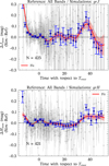 |
Fig. B.1. Jmax (top panel) and Hmax (bottom panel) residuals, between simulations with 1 NIR epoch, using grJ and grH, respectively, and reference values. The weighted mean (Δ) and uncertainty on the weighted mean (σ) in bins of 2 days are shown in blue. A ‘correction snake’ and its uncertainty are calculated by fitting the residuals with GPs (red line and shaded region); N is the total number of simulations. |
All Tables
All Figures
 |
Fig. 1. SNooPy fit of the multi-colour (uBgVriYJH) light curves of SN 2004eo. The max_model model is used throughout this work. |
| In the text | |
 |
Fig. 2. Comparison between the reference and the entire CSP samples. Top panel: redshift distribution of CSP-I + CSP-II (empty bars) and the 50 SNe Ia comprising our reference sample (orange bars). Bottom panel: sBV distribution of SNe Ia from CSP-I + CSP-II (empty bars) labelled as ‘normal’ and the reference sample (orange bars). The values of sBV were obtained by fitting the SNe with SNooPy using the max_model model. Only the ‘normal’ SNe are shown in this case as SNooPy mainly provides templates for these objects and not other types. |
| In the text | |
 |
Fig. 3. Multi-colour light curves of SNe 2004eo (top), 2005M (middle), and 2009aa (bottom) from CSP-I. |
| In the text | |
 |
Fig. 4. Multi-colour light curves of SNe LSQ12bld (top), PTF13ebh (middle; Hsiao et al. 2015), and ASASSN-14lp (bottom; Shappee et al. 2016) from CSP-II. |
| In the text | |
 |
Fig. 5. Fits of single-epoch JH simulations for ASASSN-14hu. Each colour represents a different simulation and fit for the NIR photometry of the SN. |
| In the text | |
 |
Fig. 6. Jmax (top panel) and Hmax (bottom panel) residuals, between simulations with coeval coeval J- and H-band epoch and reference value. The weighted mean and uncertainty on the weighted mean in bins of two days are shown in blue. A “correction snake” and its uncertainty are calculated by fitting the residuals with GPs (red line and shaded region), while N is the total number of simulations. |
| In the text | |
 |
Fig. 7. Jmax residuals between simulations with three coeval J- and H-band epochs and reference sample as a function of metrics (i), (ii), and (iii) (top, middle, and bottom panels, respectively). The weighted mean and uncertainty on the weighted mean in bins of two days are shown in blue for each of the panels. The residuals in Jmax do not vary much as a function of metrics (ii) and (iii), which means that metric (i) is the most relevant for estimating Jmax. The metrics are described in Sect. 4, while N is the total number of simulations. The global offsets in the middle and bottom panels are driven by those simulations with phases ≲ − 5 days and ≳30 days from the top panel. |
| In the text | |
 |
Fig. 8. Tmax comparison for cadence simulations. Top panel: difference in Tmax between the cadence simulations (Sect. 5.1) and reference sample (ΔTmax). All simulations with restframe cadences < 10 days are considered here. The weighted average Δmax is 0.01 days (vertical dotted line). Bottom panel: ΔTmax over the uncertainty in Tmax (i.e. significance) for the cadence simulations. The average significance is 0.13 (vertical dotted line), while very few simulations have a significance greater than 3.0. The average uncertainty in Tmax (0.19 days) is much larger than the weighted average ΔTmax. |
| In the text | |
 |
Fig. 9. Difference in Tmax between the cadence simulations (Sect. 5.1) and reference sample (ΔTmax) as a function of restframe cadence. The binned average and standard deviation of ΔTmax are shown as red squares with error bars. The average observed cadences for ZTF (2 days), LSST (assuming 3-day baseline cadence per filter), CSP (3.1 days for the reference sample), and DES (7 days; Brout et al. 2019) are shown as vertical dotted lines. We note that the restframe cadence is faster by a factor of 1 + z than the observed cadence; N is the total number of simulations. |
| In the text | |
 |
Fig. 10. Effect that restframe cadence (up to 10 days) in the optical gr-bands has on the estimation of the NIR peak magnitudes. The grey lines represent ΔTmax multiplied by the gradient of the NIR light-curve template bands as a function of phase, for each simulated SN from Sect. 5.1. We note that the shape of the templates depends on the value of sBV, which is obtained from the fits of the gr-band light curves. The average NIR peak magnitude offset is shown as a red line for J (top panel) and H (bottom panel) bands. The 1σ scatter in NIR peak magnitude (red shaded region) is < 0.02 mag in J band and much smaller for H band (< 0.01 mag). |
| In the text | |
 |
Fig. 11. Difference in Tmax between the cadence simulations (Sect. 5.1) and reference sample (ΔTmax) as a function of the phase of the first observation. The simulations are split in three groups according to the cadence (cad) range: 2 < cad < 5 days (purple crosses), 5 < cad < 8 days (pink circles), and 8 < cad < 10 days (gold squares). Tmax is shown as a vertical dashed line. Independent of the cadence, the scatter in ΔTmax starts rapidly increasing for the first observations with phases of ≳ − 5 days. |
| In the text | |
 |
Fig. 12. Tmax comparison for S/N simulations. Top panel: difference in Tmax between the S/N simulations (Sect. 5.2) and reference sample (ΔTmax). The weighted average ΔTmax is −0.007 days (vertical dotted line). Bottom panel: ΔTmax over the uncertainty in Tmax (i.e. significance) for the S/N simulations. The average significance is 0.23 (vertical dotted line), while very few simulations have a significance greater than 3.0. The average uncertainty in Tmax (0.12 days) is larger than the weighted average ΔTmax. |
| In the text | |
 |
Fig. 13. Difference in Tmax between the S/N simulations (Sect. 5.2) and reference sample as a function of S/N. The binned weighted mean and standard deviation of ΔTmax are shown as red squares with error bars; N is the total number of simulations. |
| In the text | |
 |
Fig. 14. Effect that S/N in the optical gr-bands has on the estimation of the NIR peak magnitudes. The grey lines represent ΔTmax multiplied by the gradient of the NIR light-curve template bands as a function of phase, for each simulated SN from Sect. 5.2. We note that the shape of the templates depends on the value of sBV, which is obtained from the fits of the gr-band light curves. The average NIR peak magnitude offset is shown as a red line for J (top panel) and H (bottom panel) bands. The 1σ scatter in NIR peak magnitude (red shaded region) is ≲0.02 mag for J band and < 0.01 mag for H band. |
| In the text | |
 |
Fig. 15. Residual in Jmax between NIR S/N simulations with J-band S/N > 21 (Sect. 5.3) and the reference sample (ΔJmax). The weighted mean and standard deviations are 0.006 mag and 0.070 mag, respectively. |
| In the text | |
 |
Fig. 16. Difference in Jmax (top panel) and Hmax (bottom panel) between the NIR S/N simulations (Sect. 5.3) and reference sample as a function of S/N. The binned median and standard deviations are shown as red squares with error bars. Simulations with all S/N values are shown in here. The average S/N of CSP SNe Ia at z > 0.08 are shown as vertical lines (21 and 8 for J and H bands, respectively); N is the total number of simulations. |
| In the text | |
 |
Fig. 17. Hubble diagram in J band. Only SNe Ia with z > 0.01 were used as the contribution from peculiar velocities is relatively small at these redshifts. The reference sample was used to fit H0 and the intrinsic dispersion (σint), keeping the peak absolute magnitude in J band (MJ = −18.5 mag) fixed. The rms for the reference sample (red) and the simulations with n = 1 (grey) are 0.166 mag and 0.180 mag, respectively. |
| In the text | |
 |
Fig. A.1. Tmax residuals (ΔTmax) between max_model and EBV_model2, using the reference sample from Section 2.3. The weighted mean of ΔTmax is ∼ − 0.001 mag (vertical black line). |
| In the text | |
 |
Fig. A.2. SNooPy fits of SN 2004eo with the EBV_model2. Note that the EBV_model2 model does not produce reliable fits of the bluest (u) and reddest (H) filters. |
| In the text | |
 |
Fig. A.3. Comparison in the uncertainty of Tmax (σ) between max_model and EBV_model2, using the reference sample from Sect. 2.3. We note that the uncertainties from the latter are larger. |
| In the text | |
 |
Fig. B.1. Jmax (top panel) and Hmax (bottom panel) residuals, between simulations with 1 NIR epoch, using grJ and grH, respectively, and reference values. The weighted mean (Δ) and uncertainty on the weighted mean (σ) in bins of 2 days are shown in blue. A ‘correction snake’ and its uncertainty are calculated by fitting the residuals with GPs (red line and shaded region); N is the total number of simulations. |
| In the text | |
Current usage metrics show cumulative count of Article Views (full-text article views including HTML views, PDF and ePub downloads, according to the available data) and Abstracts Views on Vision4Press platform.
Data correspond to usage on the plateform after 2015. The current usage metrics is available 48-96 hours after online publication and is updated daily on week days.
Initial download of the metrics may take a while.


