| Issue |
A&A
Volume 679, November 2023
|
|
|---|---|---|
| Article Number | A95 | |
| Number of page(s) | 26 | |
| Section | Cosmology (including clusters of galaxies) | |
| DOI | https://doi.org/10.1051/0004-6361/202244893 | |
| Published online | 15 November 2023 | |
An updated measurement of the Hubble constant from near-infrared observations of Type Ia supernovae⋆
1
Institute of Space Sciences (ICE, CSIC), Campus UAB, Carrer de Can Magrans, s/n, 08193 Barcelona, Spain
e-mail: This email address is being protected from spambots. You need JavaScript enabled to view it.
2
Institut d’Estudis Espacials de Catalunya (IEEC), 08034 Barcelona, Spain
3
Institute for Astronomy, University of Hawaii, 2680 Woodlawn Drive, Honolulu, HI 96822, USA
4
Space Telescope Science Institute, 3700 San Martin Drive, Baltimore, MD 21218, USA
5
Department of Physics and Astronomy, Johns Hopkins University, Baltimore, MD 21218, USA
6
Institute of Astronomy and Kavli Institute for Cosmology, University of Cambridge, Madingley Road, Cambridge CB3 0HA, UK
7
Department of Physics and Astronomy, Aarhus University, Ny Munkegade 120, 8000 Aarhus C, Denmark
8
European Southern Observatory, Karl-Schwarzschild-Strasse 2, 85748 Garching, Germany
9
Observatories of the Carnegie Institution for Science, 813 Santa Barbara St., Pasadena, CA 91101, USA
10
Department of Physics, Duke University, Durham, NC 27708, USA
11
The Oskar Klein Centre for Cosmoparticle Physics, Department of Physics, Stockholm University, 10691 Stockholm, Sweden
12
School of Physics, Trinity College Dublin, College Green, Dublin 2, Ireland
13
Department of Physics and Astronomy, Rutgers the State University of New Jersey, 136 Frelinghuysen Road, Piscataway, NJ 08854, USA
Received:
5
September
2022
Accepted:
15
September
2023
Abstract
We present a measurement of the Hubble constant (H0) using type Ia supernovae (SNe Ia) in the near-infrared (NIR) from the recently updated sample of SNe Ia in nearby galaxies with distances measured via Cepheid period-luminosity relations by the SH0ES project. We collected public near-infrared photometry of up to 19 calibrator SNe Ia and 57 SNe Ia in the Hubble flow (z > 0.01), and directly measured their peak magnitudes in the J- and H-band by Gaussian processes and spline interpolation. Calibrator peak magnitudes together with Cepheid-based distances were used to estimate the average absolute magnitude in each band, while Hubble-flow SNe were used to constrain the zero-point intercept of the magnitude–redshift relation. Our baseline result of H0 is 72.3 ± 1.4 (stat) ±1.4 (syst) km s−1 Mpc−1 in the J-band and 72.3 ± 1.3 (stat) ±1.4 (syst) km s−1 Mpc−1 in the H-band, where the systematic uncertainties include the standard deviation of up to 21 variations of the analysis, the 0.7% distance scale systematic from SH0ES Cepheid anchors, a photometric zero-point systematic, and a cosmic variance systematic. Our final measurement represents a measurement with a precision of 2.8% in both bands. Among all the analysis variants, the largest change in H0 comes from limiting the sample to those SNe from the CSP and CfA programs; they are noteworthy because they are the best calibrated, yielding H0 ∼ 75 km s−1 Mpc−1 in both bands. We explore applying stretch and reddening corrections to standardize SN Ia NIR peak magnitudes, and we demonstrate that they are still useful to reduce the absolute magnitude scatter and, which improves its standardization, at least up to the H-band. Based on our results, in order to improve the precision of the H0 measurement with SNe Ia in the NIR in the future, we would need to increase the number of calibrator SNe Ia, to be able to extend the Hubble–Lemaître diagram to higher redshift, and to include standardization procedures to help reduce the NIR intrinsic scatter.
Key words: supernovae: general / galaxies: distances and redshifts / cosmological parameters
Photometry and lightcurve fit results are available at the CDS via anonymous ftp to cdsarc.cds.unistra.fr (130.79.128.5) or via https://cdsarc.cds.unistra.fr/viz-bin/cat/J/A+A/679/A95
© The Authors 2023
 Open Access article, published by EDP Sciences, under the terms of the Creative Commons Attribution License (https://creativecommons.org/licenses/by/4.0), which permits unrestricted use, distribution, and reproduction in any medium, provided the original work is properly cited.
This article is published in open access under the Subscribe to Open model. This email address is being protected from spambots. You need JavaScript enabled to view it. to support open access publication.
1. Introduction
Determining the expansion rate of the Universe parameterized by the Hubble–Lemaître parameter H(z) has been a major endeavor in cosmology since the discovery of the expanding Universe (Lemaître 1931; Hubble 1929). The H(z) parameter is not constant, but rather varies over cosmic time following the deceleration and acceleration of the Universe. In recent years, significant effort has been made to measure with high precision the local value of the Hubble–Lemaître parameter known as the Hubble constant (H0, Jackson 2007; Freedman & Madore 2010), and today H0 is estimated in the local Universe through the distance ladder technique with an uncertainty of ∼1 km s−1 Mpc−1 (≲1.5%, Riess et al. 2022, hereafter R22). Perplexingly, these findings have revealed a dramatic discrepancy, dubbed the Hubble tension: the estimation of H0 from the local distance ladder is in strong disagreement (at 5σ or one chance in ∼3.5 million) with the value inferred at high redshift from the angular scale of fluctuations in the cosmic microwave background (CMB; Planck Collaboration VI 2020), possibly hinting toward new physics beyond the standard cosmological model. This discrepancy represents the most urgent puzzle of modern cosmology, and it is currently one of its hottest topics.
The Supernovae, H0, for the Equation of State of Dark energy (SH0ES; R22) team has been leading the effort over the last two decades, building on the initial attempts to measure H0 using the Hubble Space Telescope (HST) by the Type Ia Supernova HST Calibration Program (Saha et al. 2001) and the HST Key Project (Freedman et al. 2001). To this end, they constructed a distance ladder that consists of three rungs. In the first and nearest rung the Cepheid period–luminosity relation (Leavitt & Pickering 1912) is calibrated using galactic geometric distance anchors, such as parallaxes to those same Cepheids (Lindegren et al. 2021), detached eclipsing binaries (DEBs; Pietrzyński et al. 2019), or water masers (Reid et al. 2019). In turn, this Cepheid calibration is used in the second rung of the distance ladder to obtain distances to nearby galaxies hosting both Cepheids and type Ia supernovae (SNe Ia). The absolute magnitude of these SNe Ia in the second rung is calibrated using the distance obtained from this independent Cepheid method, and it is finally used in the third rung of the ladder to calibrate the absolute magnitude of SN Ia host galaxies at larger distances. SH0ES has recently provided the most precise direct measurement of H0 in the late Universe (R22) by calibrating galactic Cepheids from Gaia EDR3 parallaxes, masers in NGC 4258, and DEBs in the Large Magellanic Cloud, and using the HST to measure distances to 38 galaxies hosting Cepheids and 42 SNe Ia. In their analysis, optical light curves of 42 and 277 SNe Ia were used in the second and third rungs, respectively.
Optical observations of SNe Ia have been widely used in past decades to measure cosmological distances. SNe Ia are the most mature and well-exploited probes of the accelerating universe, and their use as standardisable candles provides an immediate route to measure dark energy (Riess et al. 1998; Perlmutter et al. 1999; Leibundgut 2001; Goobar & Leibundgut 2011). This ability rests on empirical relationships between SN Ia peak brightness and light curve width (Rust 1974; Pskovskii 1977; Phillips 1993), and SN color (Riess et al. 1996; Tripp 1998), which standardize the optical absolute peak magnitude of SNe Ia down to a dispersion of ∼0.12 mag (∼6% in distance; Betoule et al. 2014). However, environmental dependences, such as the mass step (Sullivan et al. 2010; Kelly et al. 2010; Lampeitl et al. 2010, but also with other global and local parameters, such as the star formation rate, metallicity, and age; see, e.g., Rigault et al. 2020; Moreno-Raya et al. 2018; Gupta et al. 2011), have been found to contribute to the systematic uncertainty budget.
Increasing evidence suggests that SNe Ia are very nearly natural standard candles at maximum light at near-infrared (NIR) wavelengths, even without corrections for light curve shape and/or reddening, and that they yield more precise distance estimates to their host galaxies than optical data alone (Elias et al. 1981, 1985; Meikle 2000; Krisciunas et al. 2004a; Wood-Vasey et al. 2008; Weyant et al. 2014; Friedman et al. 2015; Avelino et al. 2019). Compared to the optical, SNe Ia in the NIR are relatively immune to the effects of extinction and reddening by dust (extinction corrections are a factor of 4 − 6 smaller than in the optical B-band; Stanishev et al. 2018), and the correlation between peak luminosity and decline rate is much smaller (e.g., Krisciunas et al. 2004a). For instance, in a sample of 15 SNe Ia located at 0.025 < z < 0.09, Barone-Nugent et al. (2012) found a scatter of 0.09 mag (4% in distance) in the H-band without applying any corrections for host-galaxy dust extinction or K-corrections (Oke & Sandage 1968). However, SN Ia cosmology in the NIR is still less developed compared to the optical, for various reasons. Optical detectors were technologically simpler and put available before the more expensive NIR detectors. Moreover, SNe Ia are intrinsically fainter in the NIR, requiring bigger telescopes and longer integration times. Current efforts are focused on increasing the number of objects with NIR observations.
Most of the NIR SN Ia data currently available at low redshift (z < 0.1) come from the Carnegie Supernova Project (CSP, Krisciunas et al. 2017b) and the Center for Astrophysics (CfA, Friedman et al. 2015) follow-up programs, with significant contributions also from smaller programs (e.g., Barone-Nugent et al. 2012; Stanishev et al. 2018; Johansson et al. 2021). At intermediate redshift (0.2 < z < 0.6) the high-redshift subprogram of the CSP (Freedman et al. 2009) obtained YJ imaging of 35 SNe Ia up to redshift 0.7 to build an i-band rest-frame Hubble diagram. More recently, the Supernovae IA in the Near-InfraRed (RAISIN, Jones et al. 2022) project has collected HST NIR observations of 45 SNe which, complemented with Pan-STARRS Medium Deep Survey (MDS; Chambers et al. 2016) and Dark Energy Survey (DES, Brout et al. 2019) optical light curves, are used to extend the Hubble–Lemaître diagram up to redshift 0.6 in rest-frame Y-band, the farthest rest-frame NIR Hubble–Lemaître diagram ever constructed. In the near future, the Nancy Roman Space Telescope supernova program (Rose et al. 2021) with its F213 filter is expected to provide NIR rest-frame observations of SNe Ia and extend the NIR Hubble diagram from redshifts ∼0.3 in J and ∼0.1 in H, provided by the F160W HST filter, to ∼0.7 in J and ∼0.3 in H (see, e.g., Fig. 2 in Jones et al. 2022). Roman, together with RAISIN and the 24 very nearby SNe Ia from the Supernovae in the Infrared avec Hubble (SIRAH; Jha et al. 2019) HST program, will provide a full space-based NIR SN Ia Hubble–Lemaître diagram. NIR observations of SNe Ia have already been used to measure H0, the most prominent efforts being those of Burns et al. (2018) using all CSP observations and the SuperNovae in object-oriented Python (SNooPy) template fitting, and Dhawan et al. (2018, hereafter D18) by directly measuring SN Ia J-band peak magnitudes from a literature sample.
In this work we obtain an updated measurement of H0 with SNe Ia in the NIR. Building from D18, we present the following improvements: (i) we collected all available NIR light curves of SNe Ia to date with data during the rise phase that allows the measurement of their peak J- and H-band magnitudes, including updated photometry of the CSP from their third data release (Krisciunas et al. 2017a; ii) all photometry is put in the CSP photometric system by applying S-corrections; (iii) the number of SNe Ia in galaxies with Cepheid-based distances is more than doubled from 9 to 19, thanks to the recently increased sample from SH0ES; (iv) the number of SNe Ia in the Hubble flow was also increased from 27 to 52(40) in J(H); and (v) the analysis is extended to the H-band. Although the distances in the second rung of our distance ladder are based on SH0ES distances, with this independent analysis we can test whether SNe Ia in the optical introduce a bias in the H0 measurement, due to systematic uncertainties introduced in their standardization.
2. Data sample
To put constraints on the current value of the Hubble expansion using SNe Ia in the NIR, we need a sample of nearby SN Ia observed in the NIR hosted by galaxies whose distance has been independently measured using other techniques and we need a sample of SNe Ia with NIR observations located farther in the Hubble flow (z > 0.01). The peak absolute magnitude of SNe Ia in those nearby galaxies (hereafter called calibrators) can then be determined simply by measuring their peak apparent brightness, and in turn this reference-calibrated magnitude is used in the Hubble-flow SNe Ia to determine distances to their hosts.
For both distance regimes our criteria to select SNe Ia is the same: SNe Ia light curves must be sparsely sampled and have at least a NIR pre-maximum photometric point to allow for a reliable measurement of the peak magnitude. D18 represents our reference work where 36 SNe Ia were selected based on their high-quality J-band photometry. Nine of the SNe Ia exploded in galaxies whose distances were determined independently by the SH0ES project (Riess et al. 2016), while 27 were in the Hubble flow.
In this work, for the calibrator sample we make use of the recently updated sample from SH0ES (R22), which was extended from 19 to 42 SNe Ia in 38 nearby galaxies with distances measured using Cepheids. We performed a thorough search of NIR J- and H-band photometry of all SNe Ia in the latest SH0ES sample of galaxies and found that up to 19 SNe Ia (including the 9 in D18) have NIR light curves of sufficient quality to be included in this analysis. Three SNe Ia (2013dy, 2012ht, 2012fr) were initially included in Riess et al. (2016), but their photometry has been published more recently, and seven other SNe Ia were in galaxies whose Cepheid distances were presented for the first time in R22. In addition, we performed a thorough search in the literature for J- and H-band NIR photometry of SN Ia in the Hubble flow (z > 0.01) and found 57 candidate objects.
All 19 SNe Ia in the calibrator sample have J-band light curves that allows for the peak-brightness determination, however only 16 have light curves with enough quality in the H-band. Similarly, for the Hubble-flow sample, while 55 SNe Ia have good J-band light curves, 13 have an H-band light curve that does not permit the determination of the peak brightness. Our initial sample is therefore 19 and 16 SNe Ia with J- and H-band light curves in calibrator galaxies, and respectively 55 and 44 SNe Ia in the Hubble flow. The list of SNe Ia in our calibrator sample (galaxies with Cepheid distances) are listed in Table 1, while our Hubble-flow SNe Ia sample is presented in Table 2. The photometry for all objects was obtained from references listed in the last column of these tables.
Properties of the 19 SNe Ia in galaxies, with distances calibrated using Cepheids in Riess et al. (2022).
Properties of the 57 SNe Ia in Hubble-flow galaxies.
3. Methods
Our approach is based on the assumption that SNe Ia are good natural standard candles in the NIR. Their peak magnitudes derived directly from the observations are thus enough to estimate cosmological distances.
3.1. Distances and redshifts
Distances μCeph and uncertainties σCeph to galaxies in the calibrator sample are taken from R22 (listed in Table 1). Heliocentric redshifts (zhelio) and their uncertainties for galaxies in the Hubble-flow sample are obtained from the SN host galaxy catalog provided in Carr et al. (2022), which are usually consistent within |#x0394;z|< 0.0005 (corresponding to 150 km s−1) with the redshifts reported in their reference sources and in the NASA/IPAC Extragalactic Database (NED1) with a few exceptions: SN 2006kf, SN 2007ba, and SN 2008hs. In addition, five SNe had different redshifts in NED and in the reference sources, and Carr et al. (2022) differs in one or the other: for SN 2005M the Carr et al. (2022) redshift is similar to that in NED; instead, for SN 2010ai, SN 2008bf, iPTF13asv, and iPTF13azs it is more similar to the reference source. In particular, SN 2008bf has an ambiguous host because it is in the middle of two nearby galaxies, NGC 4061 and NGC 4065. In our baseline analysis we chose to use the redshifts from Carr et al. (2022). These redshifts were then converted to the 3K CMB reference frame (zCMB) and corrected for peculiar velocities (zcorr) induced by visible structures, as described in their work. We study the effect of the selection of heliocentric redshifts, CMB frame correction, and peculiar velocity correction in Sect. 5.1.
3.2. S-corrected photometry
Published J- and H-band photometry for both the calibrator and the Hubble-flow sample was S-corrected to the same photometric system using internal routines in SNooPy (v.2.5.3; Burns et al. 2015). Given that most of the objects were published by the CSP we used their photometric system as our reference system. More details about the nature of S-corrections can be found in Appendix A of Stanishev et al. (2007). In our Appendix A we show most of the filter transmission used to obtain SN Ia light curves used in this work, and the magnitude of the S-corrections for tha calibrator sample. S-corrected light curves to the CSP J and H filters are publicly available at github2.
It should be noted that for SN 2013dy, before S-correction, we first had to convert SN 2013dy published photometry in Pan et al. (2015) from the AB to the Vega system following Maíz Apellániz (2007; their Table 4),
 (1)
(1)
 (2)
(2)
3.3. Multiband SNooPy fits
We fitted UV+optical+NIR light curves of both the calibrator and the Hubble-flow samples with SNooPy, using the EBV_model2 and max_model models with #x0394;m15 as a light curve width parameter. Prior to the template fitting and within the SNooPY framework, the photometric points are corrected for Milky Way extinction using the dust maps from Schlafly & Finkbeiner (2011), and then K-corrected using the Hsiao et al. (2007) template. The K-correction involves first color-correcting the spectral energy distribution (SED) by multiplying the original template with a smooth function, which ensures that the observed colors match the synthetic colors derived from the corrected SED. Regarding K-corrections, since the redshift range of our sample is quite narrow (z < 0.04, except five objects up to z ∼ 0.08), they are in general small. At the median redshift of our sample z = 0.023 the K-correction is 0.058 mag in J and 0.030 mag in K, and up to 0.156 mag in J and 0.125 mag in H for the SN at the highest redshift (z = 0.08).
When using the EBV_model2, the fitter provides an estimate of the time of maximum in the B-band Tmax, B, the light curve width parameter #x0394;m15 in the B-band, and the color excess at peak E(B − V). Moreover, we also obtain the J- and H-band peak magnitude given by the template. However, some of these parameters are affected by covariances among bands that are intrinsic to the model (for more details, see, e.g., Uddin et al. 2020). For this reason, in this work we instead use the results from the more versatile max_model, which fits each band independently and is more convenient for the purpose of this work. We obtained the time of maximum Tmax, B and light curve width parameter #x0394;m15 in the B-band, and the J- and H-band time of maximum  and peak magnitude
  . All these parameters are listed in Appendix C.
3.4. J and H peak magnitudes
In addition to the NIR peak magnitudes from template fitting, following D18, we estimate J and H peak magnitudes through simple interpolation of their light curves. In this way, we can independently obtain these values, which include corrections for SN light curve shape and color, without relying on a particular light curve template.
We interpolated J and H light curves individually via SNooPy internal routines that rely on either Gaussian processes (GPs) using the scikit-learn package (Pedregosa et al. 2011) with a constant plus a Matérn kernel or via spline fits using FITPACK (Dierckx 1993).3 For the GP interpolation we set the timescale over which the function varies to ten days, the amplitude of typical function variations as the standard deviation of the photometric points in magnitudes in each light curve, and a smoothness of ν = 3.5. For some objects4 the GP is less reliable than a simple spline interpolation, and in our baseline calculation of H0 we chose the fit that provides the lowest χ2 between data and fit in the time range (−10,+20) days. Our best light curve fits are shown in Appendix D for both the calibrator and the Hubble-flow samples, where the GP fits are shown as solid lines and splines as dashed lines.
We obtained the peak magnitude in the X-band mX and its uncertainty σmX from the interpolated light curves, which were then corrected for Milky Way reddening using the maps of Schlafly & Finkbeiner (2011) and a Fitzpatrick (1999) extinction law with RV = 3.1, equivalent to RJ = 0.86 and RH = 0.53 and K-corrected using the SN Ia spectral energy distribution models from Hsiao et al. (2007), following the same procedure as in the SNooPy fits. The corrected peak magnitudes, the extinctions, and the K-correction terms are presented in Table 1 for the calibrator sample and in Table 2 for the Hubble-flow sample.
3.5. Absolute magnitudes
To obtain the absolute magnitudes of SNe Ia in the calibrator sample we subtract R22 Cepheid distance moduli of their host galaxies from the apparent peak magnitude,
 (3)
(3)
and add their uncertainties in quadrature,
 (4)
(4)
The final absolute magnitudes are included in Table 1.
For the Hubble-flow SNe, we subtracted the distance modulus μ(z) using a flat ΛCDM cosmology with ΩΛ = 0.7 (equivalent to a deceleration parameter q0 = Ωm/2 − ΩΛ = −0.55 and a jerk or prior deceleration j0 = 1.0; Visser 2004) and H0 = 70 km s−1 Mpc−1 from the apparent peak magnitude. For the uncertainty we added the peak magnitude error in quadrature with the redshift (zcorr) and peculiar velocity uncertainties converted to magnitudes as
 (5)
(5)
where we adopted a vpec = 250 km s−1 (de Jaeger et al. 2022).
3.6. H0 determination
To provide an estimate of H0 with SN Ia in the NIR we need to combine our calibrator sample, which constrains the absolute magnitude MX, and the Hubble-flow sample, which determines the zero-point intercept aX of the NIR SN Ia magnitude–redshift relation.
We follow here a procedure similar to that used in D18 and de Jaeger et al. (2020), and more recently in de Jaeger et al. (2022). Combining the expression of the distance modulus,
 (6)
(6)
and the kinematic expression of the luminosity distance as defined by Riess et al. (2007),
 (7)
(7)
we end up with the simple equation,
 (8)
(8)
where MX is constrained by the calibrator sample, and aX is the intercept of the distance–redshift relation given for an arbitrary expansion history and for z > 0 Riess et al. (2022), and it is determined from the Hubble-flow sample by
 (9)
(9)
To find H0 and MX we fit a joint Bayesian model to the combined dataset using the Markov chain Monte Carlo (MCMC) sampler of the posterior probability function emcee (Foreman-Mackey et al. 2013) with 200 walkers and 2000 steps each, burning the first 1000 steps per each walker, so with a total of 200 000 samples. In addition, we account for an unmodeled intrinsic NIR SN Ia scatter σint, as a nuisance parameter, which is added in quadrature to the calibrator and Hubble-flow peak magnitude uncertainty ( ;
;  ), and that we interpret as SN-to-SN variation in the peak luminosity to be constrained by the data and marginalized over. The likelihood we optimize is,
 (10)
(10)
where the calibrator term penalizes depending on how far the calibrators are to the mean absolute magnitude, and the Hubble-flow term penalizes depending on how close the Hubble-flow objects are to the mean absolute magnitude for the input H0. We use as initial guesses for the walkers a H0 = 70 km s−1 Mpc−1, a MX equal to the average calibrator absolute peak magnitude in each band, and a  , and allow them to vary on a scale of 10 km s−1 Mpc−1, 1 mag, and 0.1 mag, respectively. We also use a single scale-free prior of log(p(σint)) = −log σint with the conditions H0 > 0 and σint > 0.
4. Results
4.1. Properties of the calibrator and Hubble-flow samples
The absolute magnitudes of 19 SNe Ia in the calibrator sample in the J-band and 16 in the H-band are presented in Fig. 1. The average J- and H-band calibrator absolute magnitudes are ⟨MJ⟩=(−18.565 ± 0.025) and ⟨MH⟩=(−18.355 ± 0.023) mag. In the J-band the average absolute magnitude is only slightly brighter (by ∼0.04 mag) than that presented in D18. These calibrator absolute magnitudes show a dispersion of σcalib = 0.16 mag in both bands, which is comparable to the typical scatter found in the optical after light curve shape and color corrections. The dispersion is larger than can be accounted for by the formal uncertainties σMX, with the reduced χ2 > 5 in both bands, confirming that an additional intrinsic scatter, σint, is needed in our analysis to account for SN-to-SN luminosity variations. We discuss below that, once included, the reduced χ2 are reduced to around unity.
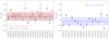 |
Fig. 1. Absolute magnitudes of the SNe Ia in the calibrator sample for the J-band (left) and H-band (right). The horizontal lines represent the weighted average and the strip the standard deviation around that value. In the left panel we included the nine SN Ia included in D18 for reference. Uncertainties correspond to those described in Sect. 3.5 and do not include the σint term added in quadrature. |
Figure 2 presents the Hubble–Lemaître diagrams and residuals of our Hubble-flow sample. We used here the redshift corrected for peculiar velocities on the X-axes, and the apparent peak magnitude of the SN in each band on the Y-axes. Hubble residuals are calculated against a flat ΛCDM cosmology with H0 = 70 km s−1 Mpc−1. Five SNe (SN 2008hs, SN 2010ai, PTF10tce (only in J), iPTF13asv (only in H), and iPTF14bdn (only in H)) were removed applying a Chauvenet criterion, which for the sample size is usually around 2.6σ, leaving the sample with 52 SNe in J-band and 40 SNe in H-band. The standard deviation of the residuals is σHF = 0.149 and 0.102 mag in the J- and H-bands, respectively. This dispersion is similar to that found with optical corrected magnitudes by SH0ES (σ = 0.135 mag; R22), and is comparable to previous works using NIR template fitting (σ = 0.116 mag in J and σ = 0.088 mag in H; Barone-Nugent et al. 2012) and interpolation (σ = 0.106 mag; D18).
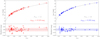 |
Fig. 2. Hubble–Lemaître diagram (top panels) and residuals (bottom panels) of our SN Ia in the Hubble-flow sample for the J-band (left) and H-band (right). The uncertainties correspond to those described in Sect. 3.5 and do not include the σint term added in quadrature. |
Figure 3 shows the cumulative distributions of #x0394;m15 and E(B − V) obtained from SNooPy fits for our calibrator and Hubble-flow samples. The shapes of their distributions and their average values are quite similar at around #x0394;m15 = 1.1 mag and E(B − V) = 0.12 mag. Both samples include objects with #x0394;m15 larger than 1.2 mag, but none of these objects reaches the value typically associated with subluminous objects (> 1.8 mag). Conversely, the color excess distribution of the calibrator sample appears to be slightly narrower than the Hubble-flow objects, with a larger median value of 0.13 mag compared to 0.07 mag for the Hubble-flow sample. We performed a two-sample Kolmogorov–Smirnov (K–S) test using the SCIPY library (Virtanen et al. 2020), and we obtained a p-value of 0.78 for #x0394;m15 and 0.15 for E(B − V), indicating that both distributions are consistent with being drawn from the same sample population. A similar figure with the cumulative distributions of the color-stretch sBV parameter is included in Appendix B.
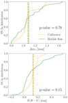 |
Fig. 3. Distributions of #x0394;m15 light curve width parameter (top) and color excess at peak E(B − V) (bottom) of the calibrator (in orange) and Hubble-flow (in green) SN Ia samples obtained from SNooPY fitting UV, optical, and NIR light curves simultaneously with the EBV_model2. Vertical dashed lines represent the average value of the distributions. The p-value of the two-sample K–S test is included in each panel. |
4.2. H0 measurement
Our baseline determination of H0 includes 19 and 16 SNe Ia from the calibrator sample, and 52 and 40 SNe Ia in the Hubble-flow sample for bands J and H, respectively. We used the R22 Cepheid distances for the calibrator sample and peculiar-velocity corrected redshifts for the Hubble-flow sample. The results from 2 × 10⁵ posterior samples of the MCMC are shown in Fig. 4 and summarized in Table 3.
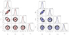 |
Fig. 4. Corner plot with the results of the MCMC posteriors of our baseline analysis. The results for the J-band are on the left and for the H-band are on the right. The red and blue contours on the scatter plots correspond to 1σ and 2σ of the 2D distributions, and the vertical and horizontal lines the medians of the posteriors. |
Results of MCMC posteriors for our baseline analysis and the 21 variations.
Our baseline result for H0 is 72.31 ± 1.42 km s−1 Mpc−1 in the J-band and 72.34 km s−1 Mpc−1 in the H-band; the errors represent the 16th and 84th percentile range, which includes 68% of the posterior samples and only include statistical uncertainties. This measurement of H0 has a ∼1.9% precision in both bands, which is lower than that found by D18 (2.2% in J). Both absolute magnitudes MX (−18.576 ± 0.036 in J and −18.349 ± 0.032 in H) are similar (within 0.01 mag) to those found by averaging out the calibrator sample magnitudes. The resulting values for the intercept ai (−2.871 ± 0.022 mag in J and −2.646 ± 0.022 mag in H) contribute less than 2% to the statistical H0 uncertainty, while the absolute magnitudes contribute around 2.5%. The additional nuisance parameter introduced in the model to account for the remaining scatter σint is found to be around 0.125 and 0.096 mag in J and H, respectively. The presence of this intrinsic scatter increases the uncertainty in the peak absolute magnitude compared to the weighted mean calculated in Sect. 4, from less than 0.01 to about 0.03 mag in both bands. As noted by D18, since the same σint is included in quadrature in the uncertainties of the calibrator and the Hubble-flow samples, MX and aX appear to be uncorrelated because they are constrained separately by each subsample.
4.3. Distance ladder
Using the values found for H0 and MX, and once σint is included in quadrature to the absolute magnitudes in both calibrator and Hubble-flow samples, we constructed the second and third rungs of the distance ladder of SN Ia in the NIR in Fig. 5. We measured the distance modulus for both calibrators and Hubble-flow SNe Ia by subtracting the average MX found with the MCMC procedure from our measured apparent peak magnitudes (on the Y-axis) against an independent measure of the distance (on the X-axis). For the calibrators we used the R22 Cepheid distances, and for objects in the Hubble flow we used the predicted distance modulus by a flat ΛCDM cosmology with ΩΛ = 0.7 and our baseline H0. The resulting scatter in the full distance ladder is 0.152 mag in the J-band and 0.122 mag in the H-band.
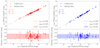 |
Fig. 5. Second and third rungs of the distance ladder for the J (left) and H (right) bands. Empty symbols represent SNe Ia in the calibrator sample, corresponding to the second rung where absolute magnitudes were calibrated from Cepheid distances. On the X-axis μ is the Cepheid-based distance from SH0ES and on the Y-axis μ is the SN Ia-based distance. The filled symbols correspond to the Hubble-flow sample (z > 0.01 in our baseline analysis) in the third rung of the distance ladder, where the X-axis μ is the SN Ia-based distance from SH0ES and the Y-axis μ is from the redshift. The symbols are different for the SNe Ia from CSP (stars), CfA (crosses), and other SNe Ia from other sources (squares and diamonds). |
Once σint is included in the uncertainty budget, we have a χ2 = 19.7 for 18 degrees of freedom (d.o.f.) in J and 26.1 for 15 d.o.f. in H for the calibrators, and a χ2 = 44.2 for 51 d.o.f. in J and 19.1 for 39 d.o.f. in H for the Hubble-flow sample, both leading to reduced χ2 around unity (0.50–1.70). Although the reduced χ2 for the calibrator sample may seem noisier than the Hubble flow, we caution that any conclusions about the scatter and χ2 is very sensitive to the exclusion of the outliers based on the Chauvenet criterion, given that our sample size is still small. Once the outliers are included, we obtain χ2/d.o.f. of 1.2 and 0.9 for the calibrator and Hubble-flow samples. One of the variations in our analysis presented in Sect. 5.1 includes the outliers removed in the baseline analysis.
5. Discussion
The main differences between this work and D18 are (i) the third and last data release of the CSP photometry from Krisciunas et al. (2017a) is used here, while D18 used the second data release from Stritzinger et al. (2011), which was available at that time; (ii) we applied S-corrections to put all compiled photometry in the same photometric system, which we chose to be the CSP system; (iii) the NIR luminosity of SNe Ia is calibrated with the NIR Cepheid distances from R22, while D18 used the NIR Cepheid distances from Riess et al. (2016). R22 not only increased the number of distances available, but also updated those from Riess et al. (2016); (iv) while the method used to determine J and H peak magnitudes is similar in the two works, the actual code for interpolation within the SNooPY framework varied from pymc included in the previous version to scipy in the current version; and (v) here we also extended the analysis to the H-band, providing an independent measurement of H0.
5.1. Analysis variations
We investigated the possible sources of systematic uncertainty in our measurements by performing some variations in the analysis, applying different cuts on the calibrator and Hubble-flow samples, and studying their effects in the determination of H0. All the results from these variations are summarized in Table 3.
5.1.1. Peculiar velocities
The first test deals with the assumed peculiar velocity uncertainty vpec added in quadrature to the magnitudes of the Hubble-flow sample. Instead of the assumed value of 250 km s−1, we tried increasing the value to 350 km s−1, took a lower value of 150 km s−1 as assumed in other works, and also tried removing this term from the analysis. The net effect of reducing the significance of this term is reducing the value of H0 by 0.15 km s−1 Mpc−1 at most, which represent a 0.2% shift with respect to the fiducial value, and passing this uncertainty to the nuisance σint parameter. All other parameters remain mostly unaltered.
5.1.2. Redshifts
The analysis was repeated, but this time changing the redshift of SNe Ia in the Hubble-flow sample. First, we used all zcmb redshifts instead of those corrected for peculiar velocities zcorr provided by Carr et al. (2022). Second, we repeated the analysis using the host galaxy redshifts reported in NED, converted to the CMB reference frame and with and without corrections for peculiar velocities using the model of Carrick et al. (2015). Finally, we repeated the process, this time starting from the redshifts reported in the reference papers, and converted to the CMB frame, and with and without Carrick et al. (2015) peculiar velocity corrections. The most significant change resulting from all these variations is a reduction in H0 to ∼1.6% in the H-band when using zcmb with no peculiar velocity corrections. Since this variation does not affect the calibration sample, we see similar changes of the aX value, and an increase in σHF and the resulting σint. Our result is in agreement with Peterson et al. (2022), who found that peculiar velocity corrections do not affect significantly the measurement of H0.
5.1.3. Extinction
The next test consisted in removing all objects with E(B − V) > 0.3, as measured from SNooPY using the EBV_model2. The SH0ES sample was selected to not have high extinction, so this cut resulted in only one object being removed from the calibrator sample (SN 2001el) and eight from the Hubble-flow sample. The effect in H0 is a change of ∼0.6% in opposite directions for each filter. Notably, since the remaining sample is less affected by reddening, σHF is reduced from 0.124 to 0.109 mag in J and is unchanged in H (0.096–0.097 mag), confirming that H-band is less affected by extinction effects.
5.1.4. Hubble-flow cut
We also tested the result of removing all objects in the Hubble-flow sample with redshifts z > 0.023, as in R22. Alternatively, we also removed the only object at z > 0.05 (PTF10ufj) to see its role in the determination of the parameters. These two cuts resulted in a reduction of the Hubble-flow sample size from 52 to 22 and 20, respectively, in the J-band and from 40 to 18 and 15 in the H-band. The resulting H0 was not significantly affected in any case for the H-band, and increases up to 1.61% for the J-band, corresponding to 01.2 km s−1 Mpc−1, becoming even more consistent with the SH0ES value.
5.1.5. Chauvenet criterion
The next test consisted in not applying in any case the Chauvenet criterion and using all the SNe Ia available including clear outliers. Adding the > 3σ outliers produces an increase in σHF from 0.149 to 0.185 mag in J and from 0.102 to 170 in H, the largest of all our variations. It also produces a 0.9 and a 0.1 km s−1 Mpc−1 reduction in H0 in the J- and H-bands, respectively.
5.1.6. Best light curve fits
In order to construct the purest sample, we tried excluding the few objects that had interpolated peak magnitude values less well constrained by visual inspection, and that could not have passed more restrictive criteria. These include SN 2008fv and SN 2003du in the calibration sample, and SN 2006hx, SN 2007ai, SN 2007bd, SN 2009bv, SN 2010ag, SN2010ai, PTF10mwb, PTF10tce, iPTF13azs, iPTF13dge, iPTF13duj, and iPTF14atg in the Hubble-flow sample. With these remaining objects, H0 is shifted down by about 0.7% in the J-band and is unchanged in the H-band.
5.1.7. GP interpolation and spline
Another test consisted of using all the SN Ia NIR peak magnitudes as obtained from the GP interpolation instead of the best between GP and spline fits. While this may be a more consistent and systematic method, we decided to choose the best fit in our baseline analysis based on the reduced χ2. As expected, this choice affects σcal by increasing the scatter up to 0.02 mag of J- and H-band calibrators, and in turn increases the value of H0 by 0.4–0.8% in both bands.
5.1.8. Light curve templates
Going one step further, we repeated the analysis, but this time we used the peak magnitudes obtained from the SNooPy template fitting using the max_model. In the previous test only those magnitudes that were obtained by the spline interpolation were modified from the baseline analysis; instead, in this case all the magnitudes were different. We find an increased dispersion in σcal in the J-band up to 0.17 mag, but a decrease in H to 0.151 mag, and a similar σHF in the J-band, but an increase in the H-band to 0.144 mag. Regarding H0, the J-band value is higher by 2.3%–73.9 km s−1 Mpc−1, and the H-band value increased by 1.3%–73.3 km s−1 Mpc−1.
5.1.9. Exclusion of subluminous SNe Ia
We also tested applying a cut in #x0394;m15 at 1.6 mag, thus excluding those objects that present wider light curves and at the fainter end of the luminosity–width relation. This is based on previous works that have shown that, similarly to the behavior in optical bands, the NIR absolute magnitudes of fast-declining SNe Ia diverge considerably from their more normal counterparts (Krisciunas et al. 2009; Kattner et al. 2012; Dhawan et al. 2017). This cut affected three objects, SN 2007ba, SN 2010Y, and iPTF13ebh in the Hubble-flow sample. As expected, the σHF is reduced to 0.144 in J and to 0.097 in H. This pulled up the H0 value by 1.2% in J, and by 0.1% in H.
5.1.10. Survey
The following three tests have to do with restricting the samples by their original source survey. We focused on the CSP and CfA for three reasons: (i) they contribute to more than half of the total sample; (ii) their data is the best and systematically well-calibrated, and includes both Hubble-flow and calibrator objects (which cancel calibration errors); and (iii) we expect more data from well-calibrated surveys to come in the near future. First, we used only SNe Ia observed by the CSP, so their photometry was not S-corrected because they were already in our reference photometric system. This includes SNe from references 6, 10, 11, and 13 in Tables 1 and 2. Next, we repeated the analysis using only those SNe Ia observed by the CfA SN program (Ref. 4 in Tables 1 and 2). Finally, we combined the data from these two surveys, discarding observations collected from other sources that were reduced differently or less systematically than in those two surveys.
When considering each survey independently, the sample sizes were reduced, especially for the calibrator sample. There are eight calibrator SNe Ia observed by the CSP5 in the J-band and six in the H-band. For CfA the corresponding numbers are four and three. For the Hubble-flow sample the reduction is not as significant; there are 29 for the CSP and 22 for CfA of the 52 SNe in the J-band, and 20 from the 40 SNe in H for both surveys. However, when the surveys are combined the numbers increase to 11 and 40 for the calibrator and Hubble-flow samples in the J-band, and 8 and 29 for the H-band, which confirms that most of the sample comes from these two surveys (50–80%).
Interestingly, in most cases the scatter of the samples is lower with respect to the baseline, with the exception of J-band CSP calibrators and the H-band CfA objects in the Hubble-flow, confirming the expectation that the more homogeneous data reduces errors, and other historic data is likely to be driving the scatter up. Particularly noteworthy is the scatter of the calibrator sample in the H-band where it is reduced from the baseline 0.160 to 0.128 mag, more in line with the Hubble flow.
The H0 values increase in all cases; the greatest was 3.4 km s−1 Mpc−1, around a 4.7% increase from the baseline value, in the case of using only CSP SNe Ia and the H-band. The main reason for the higher value of H0 is that the mean absolute magnitudes of these samples are 0.1 fainter (−18.48 mag in J and −18.27 mag in H) compared to the baseline. We attribute these differences among subsamples to past inhomogeneities of the NIR systems, filters, and zero points, among other factors. As a way around this problem, we note that in the future better calibration in the NIR will be important to improve upon these constraints.
5.1.11. Host galaxy type
Another test consisted in considering only SNe Ia that occurred in spiral galaxies, by excluding those in E and S0 host galaxies, as classified in NED. This was driven by the fact that all calibrator galaxies selected by SH0ES were star forming, in order to be able to measure Cepheid stars. In this way the resulting SNe Ia in the calibrator and Hubble-flow samples were hosted by a similar type of galaxy. For those galaxies with no morphological classification in NED, we searched for host galaxy images in PanStarrs and confirmed they were all blue extended objects with structure; we classified them all as Spiral and included them in this test. All the morphological classifications can be found in Table C.1.
In the H-band we find most of the parameters unchanged, with an increase of less than 0.1% in H0 and an increase in σint to 0.103 mag. In the J-band, H0 is increased by 1.5% from the baseline to 73.43 km s−1 Mpc−1, and σint is reduced to 0.115 mag.
5.1.12. SH0ES selection
Finally, we tried to mimic as closely as possible the cuts and selection done by SH0ES, which consisted in keeping only SNe Ia that occurred in star-forming galaxies and increasing the redshift cut of the Hubble-flow sample to z = 0.023. In this way the resulting numbers would be the most directly comparable to R22. The H0 values of this variation are 74.02 ± 1.7 and 72.32 ± 1.8 km s−1 Mpc−1 for J and H, respectively. Both are fully consistent with the R22 H0 value.
5.1.13. Summary of all variations
In summary, the largest difference of our 21 variations with respect to the baseline analysis was found when we used only objects observed by the two main surveys, CSP and CfA, obtaining an H0 of up to 75.7 km s−1 Mpc−1, a 4.7% increase. However, as mentioned above, this may be due to the small size of the resulting calibration samples and because those few objects are on average fainter than the full sample. In addition, most of the objects followed up by these projects come from targeted searches, which may be biasing SN and host galaxy properties. Future work using SNe Ia from unbiased searches may be able to quantify how important this bias is. In addition, the variations that provided the largest difference in H0 were mimicking the SH0ES selection, and using peak magnitudes from template fit. In the J-band the largest change was the SH0ES selection increasing the H0 value by 2.4% to 74.02 km s−1 Mpc−1, which highlights the effect that SNe at redshifts between the Hubble-flow cuts (0.01 < z < 0.023) may be introducing. The largest change in H is when using zcmb redshifts from the reference papers without peculiar velocity corrections, reducing the H0 value by 1.6%–71.2 km s−1 Mpc−1. In the J-band H0 is reduced by 1%–71.6 km s−1 Mpc−1. In general, we see that peculiar velocity corrections increase the vH0 value by about 0.5 km s−1 Mpc−1 independently of which z we are using. The second largest change in J and H was when using the peak magnitudes from template fitting, increasing the H0 value by 2.3%–73.9 in J and by 1.3%–73.3 km s−1 Mpc−1 in the H-band. In this case the difference highlights how important the assumptions of the template fitting are when combining optical and NIR data. The larger amount of optical data has more weight in determining light curve parameters and colors, and may not be leaving enough leverage for the NIR light curve shapes and peak magnitudes to match well.
All 21 H0 measurements from the analysis variants are consistent with our baseline result. They are all plotted in Fig. 6 as individual Gaussian distributions, together with the baseline analysis result and the 1σ vertical strips of the Planck and SH0ES H0 measurements. The median and standard deviation of all the variants is 72.72 ± 1.08 km s−1 Mpc−1 in J and 72.32 ± 1.08 km s−1 Mpc−1 in H, which corresponds to a difference of only 0.41 and 0.02 km s−1 Mpc−1 from our fiducial value (29% in J and 2% in H of the statistical uncertainty).
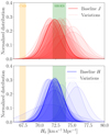 |
Fig. 6. Probability Gaussian densities of our baseline analysis (solid) and the 21 variations performed in Sect. 5.1. The two vertical strips correspond to the 1σ uncertainties around the best H0 value from the Planck Collaboration VI (2020) and the SH0ES project (R22). The results with the J-band are in the upper panel and with the H-band in the lower panel. |
5.2. Systematic uncertainties
To estimate our systematic uncertainties, we considered four different terms, and added them all in quadrature. First, following the conservative approach of Riess et al. (2019), our internal systematic uncertainty was calculated as the standard deviation of our variants. From the 21 variants presented in Table 3, we obtained a systematic uncertainty of 1.08 km s−1 Mpc−1 (1.4%) in both bands. Second, we considered the systematic distance scale error as the mean of the three SH0ES Cepheid anchors in R22 (see their Table 7). This amounts to 0.7% of the H0 value, and thus 0.51 km s−1 Mpc−1 for both bands. Third, we included a photometric zero-point systematic error between the calibrator and the Hubble-flow sample, given the fact that while the Hubble-flow sample comes mostly from the CSP and CfA, the calibrator sample is only 11 out of 19 (in J) and 8 of 16 (H) from these surveys. We consider that there can be a 1σ (∼0.04 mag) zero-point difference in the NIR between the well-calibrated systematics of CfA and CSP with respect to the literature SNe Ia, but because almost half of the calibrator sample is CfA or CSP (compared to almost all of the Hubble flow) this error reduces to 0.02 mag or 0.7 km s−1 Mpc−1. Finally, we budgeted for additional peculiar velocity uncertainties correlated on larger scales. We calculated the linear power spectrum using CLASS (Blas et al. 2011) and cosmological parameters from Planck Collaboration VI (2020). Using the formulae of Davis et al. (2011) we evaluated the correlations of our sample, and found for our sample geometry and weighting of Hubble-flow supernovae that the additional cosmic variance expected is 1.9%. Given the results of Kenworthy et al. (2022), we expect that the use of peculiar velocity corrections based on Carrick et al. (2015) will reduce this systematic by a factor of four, so we considered 0.5%, which translates into 0.4 km s−1 Mpc−1.
Adding these four terms in quadrature we obtained a systematic error of 1.44 km s−1 Mpc−1. Including both statistical and systematic uncertainties, our final H0 value is 72.31 ± 1.42 (stat) ±1.44 (sys) km s−1 Mpc−1 in J, 72.34 (stat) ±1.44 (sys) km s−1 Mpc−1 in H, or if reported as a single uncertainty, 72.31 ± 2.02 km s−1 Mpc−1 on J, and 72.34
 km s−1 Mpc−1 in H, representing a 2.8−2.7% uncertainty. Compared to D18, who obtained a statistical uncertainty of 1.6 and a systematic error of 2.7 km s−1 Mpc−1 in the J-band, the measurement found here entails a reduction of 0.2 and 0.7 km s−1 Mpc−1, respectively, in the H0 uncertainty. This is the most precise H0 value obtained from SNe Ia only with NIR data. Taking into account both sources of uncertainty, our value differs by 2.3–2.4σ from the high-redshift result of Planck Collaboration VI (2020) and by only 0.3σ from the local measurement (R22).
5.3. NIR standardization
Our determination of the NIR (J and H) peak magnitude by using GP or spline interpolation, and the subsequent determination of distance, has not been corrected by light curve and color relations in contrast to the common practice when dealing with optical data. To explore whether these corrections may be useful in the NIR to reduce the dispersion, we show in Fig. 7 relations between the absolute magnitudes of our sample and light curve parameters #x0394;m15 and E(B − V), all together for the J- and H-band. A similar plot with the sBV color-stretch parameter is included in Appendix B.
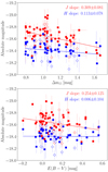 |
Fig. 7. Dependences of Hubble residuals on SN Ia light curve parameters. The open symbols correspond to SNe Ia in the calibrator sample, while the filled symbols are for those in the Hubble-flow sample. |
We note that SNe Ia with higher values of #x0394;m15 tend to be fainter in both bands. A linear regression to all values, calibrators, and Hubble-flow SNe Ia, reveals that a 3.8σ slope (0.309 ± 0.081) exists in the absolute magnitude versus the #x0394;m15 relation in the J-band, although the significance is reduced to 1.5σ (0.113 ± 0.078) in the H-band. For E(B − V) we find a 2σ slope (0.254 ± 0.125) for the J-band, and an inexistent relation (0.006 ± 0.104) for the H-band. These two results would be in agreement with these relations being of less importance as redder bands are considered, up to the point where the extinction correction is not needed in the H-band.
5.3.1. Applying Δm15 and E(B − V) corrections
Applying the stretch correction to the initial absolute magnitude of our calibrators reduces the scatter from 0.160 mag to 0.149 in J and 0.154 mag in H. Similarly, applying the reddening correction, the scatter is mostly unaltered from 0.160 to 0.159 mag in J and 0.160 mag in H. Regarding the Hubble-flow sample, the stretch correction reduces the scatter from 0.149 to 0.132 mag in J, and leaves it at 0.102 mag in H. With the reddening correction the reduction of the scatter in J is not so pronounced as with the stretch correction going from 0.149 to 0.142 mag, and it is also unaltered in H at 0.102 mag.
5.3.2. NIR H0 with corrections
The main assumption in our analysis is that SNe Ia are natural standard candles in the NIR. However, the relations found in the previous section suggest that SNe Ia NIR absolute magnitudes can still be corrected using the typical stretch and reddening relations to improve their standardization, especially in the J-band.
First, we explored the inclusion of a stretch correction to the SNe Ia peak magnitudes by adding a term,
 (11)
(11)
in the likelihood presented in Eq. (10), where α corresponds to the relation found above between absolute magnitude and stretch, and #x0394;m15 is found using the max_model SNooPy fit. We repeated the same analysis with these stretch-corrected magnitudes, using the α values found above as priors in the optimization, and the results are summarized in Table 4. The stretch correction is mostly turning the peak magnitudes a bit brighter, as can be seen in the MX and −5aX parameters being 0.01–0.03 mag brighter in the two bands. The value of H0 increases by 0.08 km s−1 Mpc−1 in J and decreases by 0.12 km s−1 Mpc−1 in H, with lower statistical errors in both cases. Interestingly, the intrinsic dispersion is reduced from 0.125 to 0.105 mag in J and from 0.096 to 0.094 mag in H. These values are consistent with those previously reported in the literature (Barone-Nugent et al. 2012), and confirm that dispersion is reduced for redder bands. Finally, the best value of the α parameter is 0.354 ± 0.086 in J and 0.133 in H, in agreement with the values found in the previous section.
Results of testing NIR standardization.
Second, we added instead a reddening correction term to the likelihood,
 (12)
(12)
where β corresponds to the relation between absolute magnitude and reddening, and E(B − V) is the EBVhost parameter from the EBV_model2 SNooPy fit. The results of this analysis, using the value of the relation found above as a prior for β, are also included in Table 4. In general, the reddening correction also turns the peak magnitudes slightly brighter, 0.01–0.03 mag for MX and −5aX in both bands, with the exception of just a few objects with a negative EBVhost parameter. In turn, the H0 value also increases by 0.06 km s−1 Mpc−1 with respect to the baseline, and the intrinsic dispersion is reduced from 0.125 to 0.112 mag in J. For the H-band, the increase in H0 is of 0.10 km s−1 Mpc−1, and the reduction of the intrinsic dispersion is 0.002 mag, similarly to the stretch correction, to 0.094 mag. In this case the β parameter is 0.338 in J and 0.108
![Mathematical equation: $ ^{+0.116]}_{-0.121} $](/articles/aa/full_html/2023/11/aa44893-22/aa44893-22-eq243.gif) in H, also consistent with the relation presented in Fig. 7.
in H, also consistent with the relation presented in Fig. 7.
Finally, we repeated the analysis adding the two corrections at the same time and minimizing α and β simultaneously; the results are also given in Table 4. In this case MX and −5aX are even brighter with changes up to 0.07 mag in J and 0.02 mag in H, while the change in H0 is only 0.06 and 0.02 km s−1 Mpc−1 in J and H, respectively. The most significant improvement is in the intrinsic scatter, which is reduced to 0.095 mag in J and 0.092 mag in H, the lowest of the four analyses. The two nuisance parameters α and β take values that are similar to those found when accounted for those corrections separately.
This test demonstrates that the stretch correction is still needed in the NIR, at least in the J (∼4σ) and H (∼1.5σ) bands, although their importance becomes lower for redder bands. In addition, the reddening correction is still significant in the J-band (∼3σ), and starts to be insignificant in the H-band (< 1σ), although the intrinsic scatter is still reduced by 0.002 mag when included. It is important to note that, even if these corrections have little effect, they have the virtue of correcting to first order for demographic differences between the calibrator and Hubble-flow samples.
6. Summary and conclusions
In this work we presented an updated measurement of the Hubble constant H0 using a compilation of published SNe Ia observations in the NIR. All the SNe in our sample were observed before their maximum, so to estimate their peak magnitudes we performed Gaussian process and spline interpolations. Combining SNe Ia in nearby galaxies whose distance has already been determined by the SH0ES team using the Cepheid period-luminosity relation, with SNe Ia at greater distances, we obtain an H0 of 72.31 ± 1.42 km s−1 Mpc−1 in the J-band and 72.34 km s−1 Mpc−1 in the H-band, where all uncertainties are statistical.
We performed up to 21 variations to our baseline analysis to estimate systematic uncertainties, and found that all are consistent with our baseline analysis. The median H0 value and dispersion of the 21 variations is 72.72 ± 1.08 km s−1 Mpc−1 in J and 72.32 ± 1.08 km s−1 Mpc−1 in H, which differs by less than 0.4 km s−1 Mpc−1 from the baseline. The largest differences in H0 of these variations with the value from the baseline analysis come from using data from a single survey, varying zcmb values (directly from publications or from large databases), applying peculiar velocity corrections, or when using template fitting instead of direct interpolation, with differences in H0 of up to 4.7%.
Taking into account up to four sources of systematic uncertainty added in quadrature, namely the dispersion of the 21 variations, the distance scale error of the three SH0ES Cepheid anchors in R22, a photometric zero-point error between the calibrator and the Hubble-flow sample, and additional peculiar velocity uncertainties correlated on larger scales, our final result of H0 is 72.31 ± 2.02 km s−1 Mpc−1 on J (2.8% uncertainty), and 72.34 km s−1 Mpc−1 in H (2.7% uncertainty), both below the 3% precision.
Our measurement is in agreement with R22 at 0.3σ, which used the same Cepheid-based distances, but used optical SN Ia data in the third rung of the distance scale, and disagrees with the Planck Collaboration VI (2020) value at 2.3–2.4σ. This independent analysis confirms both that SNe Ia in the optical do not introduce any bias in the H0 measurement due to systematic uncertainties introduced in their standardization, and that using SNe Ia in the NIR is a powerful tool for cosmological analysis.
Figure 8 shows the reference H0 measurements from the Planck Collaboration VI (2020) and R22 as vertical strips, together with our results with SNe Ia in the NIR with the J- and H-bands, and a summary of other recent independent measurements obtained with the tip of the red giant branch (TRGB; Freedman 2021; Anand et al. 2022; Scolnic et al. 2023), type II supernovae (SNe II; de Jaeger et al. 2022), surface brightness fluctuations (SBFs; Blakeslee et al. 2021), MIRAS (Huang et al. 2020), strong lenses (HOLiCOW; Wong et al. 2020), the Megamaser Cosmology Project (MCP; Pesce et al. 2020), and by the Dark Energy Survey combining clustering and weak lensing data with baryon acoustic oscillations and Big Bang nucleosynthesis (Abbott et al. 2018). It can clearly be seen how the precision of our measurement is competitive compared to other probes.
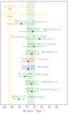 |
Fig. 8. Summary plot of the latest measurements of H0 using several different techniques from the early (in orange) and late (in green) Universe. The vertical colored strips represent the reference early Universe value by the Planck satellite and the late Universe value from SH0ES. The late Universe measurements are sorted by the size of the uncertainty, from top to bottom. Our measurements are included in red (for J) and blue (for H). |
We explored the standardization of SN Ia NIR absolute magnitudes by including a term that accounts for the light curve width and color excess (obtained from optical+NIR SNooPy fits). All tests point in the direction of reducing the uncertainty in H0, the dispersion of the absolute magnitudes, and the intrinsic scatter when performing the H0 minimization. The nuisance parameters α and β that describe the relations between absolute magnitudes and light curve parameters are much smaller, but still significant (especially for J) compared to optical bands. Even if these corrections have little effect, they have the virtue of correcting to first order for demographic differences between the calibrator and Hubble-flow samples.
Based on our results, in order to improve the precision in H0 we will need to do the following: (i) increase the number of calibrators, which translates into obtaining high-quality NIR data of SNe Ia occurring in very nearby galaxies for which any of these independent techniques can be used to determine its distance. In particular, the James Webb Space Telescope will naturally take over from the effort made by the HST in obtaining NIR Cepheid imaging of more in number and also farther galaxies to increase independent Cepheid-based distances of SN Ia hosts; (ii) increase the number of well-observed Hubble-flow SNe Ia. In this regard, the future Nancy Roman Space Telescope, with its wide field of view and the F213 filter, will provide a large number of NIR light curves of SNe Ia at higher redshift, allowing a full JH rest-frame NIR Hubble–Lemaître diagram of SNe Ia up to redshifts of 0.7; and (iii) study further the NIR standardization of SN Ia light curves in order to reduce the scatter of their absolute peak magnitudes, and therefore their distance estimation. As suggested by our test in Sect. 5.3, some improvement is possible by taking into account light curve parameters, but more work is definitely needed to determine this more reliably; and (iv) other improvements include, to name a few, better NIR spectral templates to obtain more precise K-corrections (Hsiao et al. 2019; Jha et al. 2020), more standard filter transmissions in the NIR to improve the accuracy of S-corrections to data obtained from different instruments, and considering the variable or individual reddening law that affects each SN individually (González-Gaitán et al. 2021).
In this work we use version 2.5.3 of SNooPy, which is written in Python 3. Previous versions based on Python 2 used PYMC for GP interpolation, but it was replaced in newer versions of SNooPy since it was not compatible with Python 3.
32(56)% in J(H) for the calibration sample, and 16(30)% in J(H) for the Hubble-flow sample.
Here we include SN 2012fr, SN 2012ht, and SN 2015F, which were observed during the second stage of the CSP (CSP-II), and so reduced following the same procedure as for all CSP-I objects, but published in individual papers by the CSP collaboration.
Acknowledgments
We acknowledge the referee for useful comments that have improved the first version of this manuscript. L.G. acknowledges financial support from the Spanish Ministerio de Ciencia e Innovación (MCIN), the Agencia Estatal de Investigación (AEI) 10.13039/501100011033, and the European Social Fund (ESF) “Investing in your future” under the 2019 Ramón y Cajal program RYC2019-027683-I and the PID2020-115253GA-I00 HOSTFLOWS project, from Centro Superior de Investigaciones Científicas (CSIC) under the PIE project 20215AT016, and the program Unidad de Excelencia María de Maeztu CEX2020-001058-M. K.M. is funded by the EU H2020 ERC grant no. 758638. M.D.S. acknowledges funding from the Independent Research Fund Denmark (IRFD, grant number 10.46540/2032-00022B).
References
- Abbott, T. M. C., Abdalla, F. B., Annis, J., et al. 2018, MNRAS, 480, 3879 [Google Scholar]
- Anand, G. S., Tully, R. B., Rizzi, L., Riess, A. G., & Yuan, W. 2022, ApJ, 932, 15 [NASA ADS] [CrossRef] [Google Scholar]
- Avelino, A., Friedman, A. S., Mandel, K. S., et al. 2019, ApJ, 887, 106 [Google Scholar]
- Barone-Nugent, R. L., Lidman, C., Wyithe, J. S. B., et al. 2012, MNRAS, 425, 1007 [NASA ADS] [CrossRef] [Google Scholar]
- Barone-Nugent, R. L., Lidman, C., Wyithe, J. S. B., et al. 2013, MNRAS, 432, L90 [NASA ADS] [CrossRef] [Google Scholar]
- Betoule, M., Kessler, R., Guy, J., et al. 2014, A&A, 568, A22 [NASA ADS] [CrossRef] [EDP Sciences] [Google Scholar]
- Biscardi, I., Brocato, E., Arkharov, A., et al. 2012, A&A, 537, A57 [NASA ADS] [CrossRef] [EDP Sciences] [Google Scholar]
- Blakeslee, J. P., Jensen, J. B., Ma, C.-P., Milne, P. A., & Greene, J. E. 2021, ApJ, 911, 65 [NASA ADS] [CrossRef] [Google Scholar]
- Blas, D., Lesgourgues, J., & Tram, T. 2011, J. Cosmol. Astropart. Phys., 2011, 034 [CrossRef] [Google Scholar]
- Brout, D., Sako, M., Scolnic, D., et al. 2019, ApJ, 874, 106 [NASA ADS] [CrossRef] [Google Scholar]
- Burns, C. R., Stritzinger, M., Phillips, M. M., et al. 2014, ApJ, 789, 32 [Google Scholar]
- Burns, C. R., Stritzinger, M., Phillips, M. M., et al. 2015, Astrophysics Source Code Library [record ascl:1505.023] [Google Scholar]
- Burns, C. R., Parent, E., Phillips, M. M., et al. 2018, ApJ, 869, 56 [Google Scholar]
- Carr, A., Davis, T. M., Scolnic, D., et al. 2022, PASA, 39 [CrossRef] [Google Scholar]
- Carrick, J., Turnbull, S. J., Lavaux, G., & Hudson, M. J. 2015, MNRAS, 450, 317 [Google Scholar]
- Cartier, R., Hamuy, M., Pignata, G., et al. 2014, ApJ, 789, 89 [NASA ADS] [CrossRef] [Google Scholar]
- Cartier, R., Sullivan, M., Firth, R. E., et al. 2017, MNRAS, 464, 4476 [NASA ADS] [CrossRef] [Google Scholar]
- Chambers, K. C., Magnier, E. A., Metcalfe, N., et al. 2016, ArXiv e-prints [arXiv:1612.05560] [Google Scholar]
- Contreras, C., Hamuy, M., Phillips, M. M., et al. 2010, AJ, 139, 519 [Google Scholar]
- Contreras, C., Phillips, M. M., Burns, C. R., et al. 2018, ApJ, 859, 24 [NASA ADS] [CrossRef] [Google Scholar]
- Davis, T. M., Hui, L., Frieman, J. A., et al. 2011, ApJ, 741, 67 [NASA ADS] [CrossRef] [Google Scholar]
- de Jaeger, T., Stahl, B. E., Zheng, W., et al. 2020, MNRAS, 496, 3402 [NASA ADS] [CrossRef] [Google Scholar]
- de Jaeger, T., Galbany, L., Riess, A. G., et al. 2022, MNRAS, 514, 4620 [NASA ADS] [CrossRef] [Google Scholar]
- Dhawan, S., Leibundgut, B., Spyromilio, J., & Blondin, S. 2017, A&A, 602, A118 [NASA ADS] [CrossRef] [EDP Sciences] [Google Scholar]
- Dhawan, S., Jha, S. W., & Leibundgut, B. 2018, A&A, 609, A72 [NASA ADS] [CrossRef] [EDP Sciences] [Google Scholar]
- Dierckx, P. 1993, Curve and Surface Fitting with Splines (New York: Clarendon Press) [CrossRef] [Google Scholar]
- Elias, J. H., Frogel, J. A., Hackwell, J. A., & Persson, S. E. 1981, ApJ, 251, L13 [NASA ADS] [CrossRef] [Google Scholar]
- Elias, J. H., Matthews, K., Neugebauer, G., & Persson, S. E. 1985, ApJ, 296, 379 [NASA ADS] [CrossRef] [Google Scholar]
- Fitzpatrick, E. L. 1999, PASP, 111, 63 [Google Scholar]
- Foreman-Mackey, D., Hogg, D. W., Lang, D., & Goodman, J. 2013, PASP, 125, 306 [Google Scholar]
- Freedman, W. L. 2021, ApJ, 919, 16 [NASA ADS] [CrossRef] [Google Scholar]
- Freedman, W. L., & Madore, B. F. 2010, ARA&A, 48, 673 [Google Scholar]
- Freedman, W. L., Madore, B. F., Gibson, B. K., et al. 2001, ApJ, 553, 47 [Google Scholar]
- Freedman, W. L., Burns, C. R., Phillips, M. M., et al. 2009, ApJ, 704, 1036 [Google Scholar]
- Friedman, A. S., Wood-Vasey, W. M., Marion, G. H., et al. 2015, ApJS, 220, 9 [NASA ADS] [CrossRef] [Google Scholar]
- Galbany, L., Ashall, C., Höflich, P., et al. 2019, A&A, 630, A76 [NASA ADS] [CrossRef] [EDP Sciences] [Google Scholar]
- González-Gaitán, S., de Jaeger, T., Galbany, L., et al. 2021, MNRAS, 508, 4656 [CrossRef] [Google Scholar]
- Goobar, A., & Leibundgut, B. 2011, Ann. Rev. Nucl. Part. Sci., 61, 251 [NASA ADS] [CrossRef] [Google Scholar]
- Gupta, R. R., D’Andrea, C. B., Sako, M., et al. 2011, ApJ, 740, 92 [Google Scholar]
- Hsiao, E. Y., Conley, A., Howell, D. A., et al. 2007, ApJ, 663, 1187 [Google Scholar]
- Hsiao, E. Y., Phillips, M. M., Marion, G. H., et al. 2019, PASP, 131, 014002 [NASA ADS] [CrossRef] [Google Scholar]
- Huang, C. D., Riess, A. G., Yuan, W., et al. 2020, ApJ, 889, 5 [Google Scholar]
- Hubble, E. 1929, Proc. Natl. Acad. Sci., 15, 168 [Google Scholar]
- Jackson, N. 2007, Liv. Rev. Relat., 10, 4 [NASA ADS] [CrossRef] [Google Scholar]
- Jha, S. W., Avelino, A., Burns, C., et al. 2019, Supernovaein the Infrared avec Hubble, HST Proposal. Cycle 27, 15889 [Google Scholar]
- Jha, S. W., Avelino, A., Burns, C., et al. 2020, Supernovaein the Infrared avec Hubble, HST Proposal. Cycle 28, 16234 [Google Scholar]
- Johansson, J., Cenko, S. B., Fox, O. D., et al. 2021, ApJ, 923, 237 [NASA ADS] [CrossRef] [Google Scholar]
- Jones, D. O., Mandel, K. S., Kirshner, R. P., et al. 2022, ApJ, 933, 172 [NASA ADS] [CrossRef] [Google Scholar]
- Kattner, S., Leonard, D. C., Burns, C. R., et al. 2012, PASP, 124, 114 [NASA ADS] [CrossRef] [Google Scholar]
- Kelly, P. L., Hicken, M., Burke, D. L., Mandel, K. S., & Kirshner, R. P. 2010, ApJ, 715, 743 [Google Scholar]
- Kenworthy, W. D., Riess, A. G., Scolnic, D., et al. 2022, ApJ, 935, 83 [NASA ADS] [CrossRef] [Google Scholar]
- Krisciunas, K., Suntzeff, N. B., Candia, P., et al. 2003, AJ, 125, 166 [NASA ADS] [CrossRef] [Google Scholar]
- Krisciunas, K., Phillips, M. M., & Suntzeff, N. B. 2004a, ApJ, 602, L81 [NASA ADS] [CrossRef] [Google Scholar]
- Krisciunas, K., Phillips, M. M., Suntzeff, N. B., et al. 2004b, AJ, 127, 1664 [NASA ADS] [CrossRef] [Google Scholar]
- Krisciunas, K., Suntzeff, N. B., Phillips, M. M., et al. 2004c, AJ, 128, 3034 [NASA ADS] [CrossRef] [Google Scholar]
- Krisciunas, K., Marion, G. H., Suntzeff, N. B., et al. 2009, AJ, 138, 1584 [Google Scholar]
- Krisciunas, K., Contreras, C., Burns, C. R., et al. 2017a, AJ, 154, 211 [NASA ADS] [CrossRef] [Google Scholar]
- Krisciunas, K., Suntzeff, N. B., Espinoza, J., et al. 2017b, Res. Notes Am. Astron. Soc., 1, 36 [Google Scholar]
- Lampeitl, H., Smith, M., Nichol, R. C., et al. 2010, ApJ, 722, 566 [Google Scholar]
- Leavitt, H. S., & Pickering, E. C. 1912, Harvard College Obs. Circ., 173, 1 [NASA ADS] [Google Scholar]
- Leibundgut, B. 2001, ARA&A, 39, 67 [NASA ADS] [CrossRef] [Google Scholar]
- Lemaître, G. 1931, MNRAS, 91, 490 [CrossRef] [Google Scholar]
- Lindegren, L., Bastian, U., Biermann, M., et al. 2021, A&A, 649, A4 [EDP Sciences] [Google Scholar]
- Maíz Apellániz, J. 2007, ASP Conf. Ser., 364, 227 [Google Scholar]
- Marion, G. H., Brown, P. J., Vinkó, J., et al. 2016, ApJ, 820, 92 [NASA ADS] [CrossRef] [Google Scholar]
- Matheson, T., Joyce, R. R., Allen, L. E., et al. 2012, ApJ, 754, 19 [NASA ADS] [CrossRef] [Google Scholar]
- Meikle, W. P. S. 2000, MNRAS, 314, 782 [NASA ADS] [CrossRef] [Google Scholar]
- Moreno-Raya, M. E., Galbany, L., López-Sánchez, Á. R., et al. 2018, MNRAS, 476, 307 [NASA ADS] [CrossRef] [Google Scholar]
- Oke, J. B., & Sandage, A. 1968, ApJ, 154, 21 [NASA ADS] [CrossRef] [Google Scholar]
- Pan, Y. C., Foley, R. J., Kromer, M., et al. 2015, MNRAS, 452, 4307 [CrossRef] [Google Scholar]
- Pedregosa, F., Varoquaux, G., Gramfort, A., et al. 2011, J. Mach. Learn. Res., 12, 2825 [Google Scholar]
- Perlmutter, S., Aldering, G., Goldhaber, G., et al. 1999, ApJ, 517, 565 [Google Scholar]
- Pesce, D. W., Braatz, J. A., Reid, M. J., et al. 2020, ApJ, 891, L1 [Google Scholar]
- Peterson, E. R., Kenworthy, W. D., Scolnic, D., et al. 2022, ApJ, 938, 112 [NASA ADS] [CrossRef] [Google Scholar]
- Phillips, M. M. 1993, ApJ, 413, L105 [Google Scholar]
- Pietrzyński, G., Graczyk, D., Gallenne, A., et al. 2019, Nature, 567, 200 [Google Scholar]
- Planck Collaboration VI. 2020, A&A, 641, A6 [NASA ADS] [CrossRef] [EDP Sciences] [Google Scholar]
- Pskovskii, I. P. 1977, Sov. Astron., 21, 675 [NASA ADS] [Google Scholar]
- Reid, M. J., Menten, K. M., Brunthaler, A., et al. 2019, ApJ, 885, 131 [Google Scholar]
- Riess, A. G., Press, W. H., & Kirshner, R. P. 1996, ApJ, 473, 88 [Google Scholar]
- Riess, A. G., Filippenko, A. V., Challis, P., et al. 1998, AJ, 116, 1009 [Google Scholar]
- Riess, A. G., Strolger, L.-G., Casertano, S., et al. 2007, ApJ, 659, 98 [NASA ADS] [CrossRef] [Google Scholar]
- Riess, A. G., Macri, L. M., Hoffmann, S. L., et al. 2016, ApJ, 826, 56 [Google Scholar]
- Riess, A. G., Casertano, S., Yuan, W., Macri, L. M., & Scolnic, D. 2019, ApJ, 876, 85 [Google Scholar]
- Riess, A. G., Yuan, W., Macri, L. M., et al. 2022, ApJ, 934, L7 [NASA ADS] [CrossRef] [Google Scholar]
- Rigault, M., Brinnel, V., Aldering, G., et al. 2020, A&A, 644, A176 [NASA ADS] [CrossRef] [EDP Sciences] [Google Scholar]
- Rodrigo, C., & Solano, E. 2020, in XIV.0 Scientific Meeting(virtual) of the Spanish Astronomical Society, 182 [Google Scholar]
- Rose, B. M., Baltay, C., Hounsell, R., et al. 2021, ArXiv e-prints [arXiv:2111.03081] [Google Scholar]
- Rust, B. W. 1974, PhD Thesis, Oak Ridge National Laboratory, Tennessee, USA [Google Scholar]
- Saha, A., Sandage, A., Tammann, G. A., et al. 2001, ApJ, 562, 314 [NASA ADS] [CrossRef] [Google Scholar]
- Schlafly, E. F., & Finkbeiner, D. P. 2011, ApJ, 737, 103 [Google Scholar]
- Scolnic, D., Riess, A. G., Wu, J., et al. 2023, ApJ, 954, L31 [NASA ADS] [CrossRef] [Google Scholar]
- Stanishev, V., Goobar, A., Benetti, S., et al. 2007, A&A, 469, 645 [NASA ADS] [CrossRef] [EDP Sciences] [Google Scholar]
- Stanishev, V., Goobar, A., Amanullah, R., et al. 2018, A&A, 615, A45 [NASA ADS] [CrossRef] [EDP Sciences] [Google Scholar]
- Stritzinger, M. D., Phillips, M. M., Boldt, L. N., et al. 2011, AJ, 142, 156 [Google Scholar]
- Sullivan, M., Conley, A., Howell, D. A., et al. 2010, MNRAS, 406, 782 [NASA ADS] [Google Scholar]
- Tripp, R. 1998, A&A, 331, 815 [NASA ADS] [Google Scholar]
- Uddin, S. A., Burns, C. R., Phillips, M. M., et al. 2020, ApJ, 901, 143 [NASA ADS] [CrossRef] [Google Scholar]
- Virtanen, P., Gommers, R., Oliphant, T. E., et al. 2020, Nat. Methods, 17, 261 [Google Scholar]
- Visser, M. 2004, Class. Quant. Grav., 21, 2603 [NASA ADS] [CrossRef] [Google Scholar]
- Wang, L., Contreras, C., Hu, M., et al. 2020, ApJ, 904, 14 [NASA ADS] [CrossRef] [Google Scholar]
- Weyant, A., Wood-Vasey, W. M., Allen, L., et al. 2014, ApJ, 784, 105 [NASA ADS] [CrossRef] [Google Scholar]
- Wong, K. C., Suyu, S. H., Chen, G. C. F., et al. 2020, MNRAS, 498, 1420 [Google Scholar]
- Wood-Vasey, W. M., Friedman, A. S., Bloom, J. S., et al. 2008, ApJ, 689, 377 [NASA ADS] [CrossRef] [Google Scholar]
Appendix A: Near-infrared filters and transmissions
All SN Ia observations used in this work were obtained from the ground at several observatories throughout the world using different combinations of telescopes, instruments, and filters (see Table A.1 for a list), with different characteristics (e.g., weather conditions, sky contamination, detector sensitivity, detector pixel size); they were reduced using different methods, software, and procedures. Our starting point for the analysis presented in this paper is the SN Ia photometry as it was published in each reference, sometimes in the natural system and other times calibrated to a known sytem (e.g., CSP, 2MASS). As described in section 3.2, we applied S-corrections in most cases to convert instrumental photometry or photometry in other systems to the CSP photometric system since that was the system with more data available.
Summary of telescopes and instruments used to obtain NIR imaging of SNe Ia used in this work.
In Figure A.1 we show 16 of the 24 J- and H-band transmissions listed in Table A.1 that were available through the Spanish Virtual Observatory filter profile service (SVO; Rodrigo & Solano 2020. Each panel shows only four transmissions per band for the sake of clarity. It is evident that transmission functions show quite a variety of shapes. In the top panel the four filters correspond to those used by the CSP collaboration, together with the Fourstar filters in the second panel, for the first (CSP-I) and second (CSP-II) stages of the project. The observed high level of homogeneity within the filters, coupled with the fact that a substantial portion of our SN data comes from this survey, justifies our selection of these bands as the reference in our study. To give an idea of the magnitude of this correction, in Figure A.2 we show the S-corrections applied within SNooPY to the 11 SNe Ia in the calibration sample that were not observed in the CSP system. The largest correction is about 0.12 mag after 10 days from the B-band maximum for the 2MASS bands, but around J and H maxima the S-correction is as big as 0.01 mag in J and 0.04 mag in H, exactly the number reported by Contreras et al. (2010) to convert between the 2MASS and CSP systems, and consistent with the recalculation done in Friedman et al. (2015).
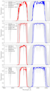 |
Fig. A.1. Responses of some of the J- (red) and H-band (blue) filters used in our sample. All transmissions were obtained from the Spanish Virtual Observatory filter profile service (SVO; Rodrigo & Solano 2020). |
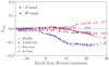 |
Fig. A.2. S-corrections of all the SNe Ia in our calibrator sample that were not observed in the CSP system. |
Appendix B: The sBV parameter
The sBV parameter combines aspects of the typical stretch and color parameters because it is calculated as the stretch factor of the B − V color-curve relative to the standard behavior of a SN Ia with a  of 30 days. It offers a more meaningful interpretation of SN Ia light curves as it measures the time at which iron recombines from [FeIII] to [FeII] (Burns et al. 2014). Importantly, it resolves the degeneracy in the relation between peak brightness and light curve width for the fainter SNe Ia (Galbany et al. 2019). The sBV values for the entire sample used in this paper are provided in Table C.1.
For completeness, we examined whether the calibrator and Hubble-flow SN Ia samples are compatible in terms of this parameter, as we did with #x0394;m15 and E(B − V) in section 5.3. The right panel of Figure B.1 shows the cumulative distribution of the color-stretch parameter sBV for the calibrator and Hubble-flow samples. The two samples exhibit a similar average sBV around 1.0, and the two-sample K-S test yields a p-value of 0.53, indicating that the distributions are consistent with being drawn from the same population.
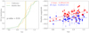 |
Fig. B.1. Dependences of Hubble residuals on SN Ia light curve parameters. The open symbols correspond to SNe Ia in the calibrator sample; the filled symbols are for those in the Hubble-flow sample. |
Similarly to the test performed in section 4.1, we also examined whether a relation between the NIR peak magnitude and sBV could be used to reduce the dispersion in peak magnitudes and thereby standardize SN Ia in the NIR. The right panel of Figure B.1 illustrates this relation, showing that brighter SNe Ia tend to have larger sBV values, meaning the peak in the B − V color-curve occurs 30 days after peak brightness. Performing a linear regression for each band independently results in a slope of -0.498±0.110 in J and -0.229±0.113 in H. These values correspond to 4.5σ and 2.0σ, respectively. This confirms that in J there is still a significant benefit in standardizing SNe Ia, while in H it is less critical.
By linearly applying the color-stretch correction to the absolute magnitudes of our calibrators, we observed a reduction in scatter from 0.160 mag to 0.149 mag in J and from 0.154 mag to 0.146 mag in H. This reduction is approximately 0.010 mag better compared to applying the #x0394;m15 correction. For the Hubble-flow sample, the stretch correction resulted in a scatter reduction from 0.149 mag to 0.130 mag in J, which is only 0.002 mag less than the #x0394;m15 correction. In H-band the scatter remained at 0.102 mag after applying the sBV correction. Overall, applying the color-stretch correction led to improvements in scatter reduction for both the calibrators and the Hubble-flow sample, particularly in J-band, confirming that it is a valuable standardization method.
Appendix C: SNooPy results
Template fitting results for SNooPy max_model and EBV_model2 (only for the E(B − V) parameter).
Appendix D: Light curves
Figure D.1 shows the J- and H-band light curves of the 19 SNe in our calibration sample along with the Gaussian process (solid lines) or spline best fits (dashed lines) used to derive peak magnitudes. In Figure D.2 similar plots are presented for the Hubble-flow sample.
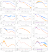 |
Fig. D.1. All calibrator Gaussian process fits (solid lines) or spline fits (dashed lines) in J-band (red) and H-band (blue). |
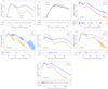 |
Fig. D.1. Continued. |
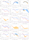 |
Fig. D.2. All Hubble-flow Gaussian process fits (solid lines) or spline fits (dashed lines) in J-band (red) and H-band (blue). |
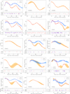 |
Fig. D.2. Continued. |
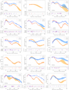 |
Fig. D.2. Continued. |
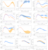 |
Fig. D.2. Continued. |
All Tables
Properties of the 19 SNe Ia in galaxies, with distances calibrated using Cepheids in Riess et al. (2022).
Summary of telescopes and instruments used to obtain NIR imaging of SNe Ia used in this work.
Template fitting results for SNooPy max_model and EBV_model2 (only for the E(B − V) parameter).
All Figures
|
Fig. 1. Absolute magnitudes of the SNe Ia in the calibrator sample for the J-band (left) and H-band (right). The horizontal lines represent the weighted average and the strip the standard deviation around that value. In the left panel we included the nine SN Ia included in D18 for reference. Uncertainties correspond to those described in Sect. 3.5 and do not include the σint term added in quadrature. |
| In the text | |
|
Fig. 2. Hubble–Lemaître diagram (top panels) and residuals (bottom panels) of our SN Ia in the Hubble-flow sample for the J-band (left) and H-band (right). The uncertainties correspond to those described in Sect. 3.5 and do not include the σint term added in quadrature. |
| In the text | |
|
Fig. 3. Distributions of #x0394;m15 light curve width parameter (top) and color excess at peak E(B − V) (bottom) of the calibrator (in orange) and Hubble-flow (in green) SN Ia samples obtained from SNooPY fitting UV, optical, and NIR light curves simultaneously with the EBV_model2. Vertical dashed lines represent the average value of the distributions. The p-value of the two-sample K–S test is included in each panel. |
| In the text | |
|
Fig. 4. Corner plot with the results of the MCMC posteriors of our baseline analysis. The results for the J-band are on the left and for the H-band are on the right. The red and blue contours on the scatter plots correspond to 1σ and 2σ of the 2D distributions, and the vertical and horizontal lines the medians of the posteriors. |
| In the text | |
|
Fig. 5. Second and third rungs of the distance ladder for the J (left) and H (right) bands. Empty symbols represent SNe Ia in the calibrator sample, corresponding to the second rung where absolute magnitudes were calibrated from Cepheid distances. On the X-axis μ is the Cepheid-based distance from SH0ES and on the Y-axis μ is the SN Ia-based distance. The filled symbols correspond to the Hubble-flow sample (z > 0.01 in our baseline analysis) in the third rung of the distance ladder, where the X-axis μ is the SN Ia-based distance from SH0ES and the Y-axis μ is from the redshift. The symbols are different for the SNe Ia from CSP (stars), CfA (crosses), and other SNe Ia from other sources (squares and diamonds). |
| In the text | |
|
Fig. 6. Probability Gaussian densities of our baseline analysis (solid) and the 21 variations performed in Sect. 5.1. The two vertical strips correspond to the 1σ uncertainties around the best H0 value from the Planck Collaboration VI (2020) and the SH0ES project (R22). The results with the J-band are in the upper panel and with the H-band in the lower panel. |
| In the text | |
|
Fig. 7. Dependences of Hubble residuals on SN Ia light curve parameters. The open symbols correspond to SNe Ia in the calibrator sample, while the filled symbols are for those in the Hubble-flow sample. |
| In the text | |
|
Fig. 8. Summary plot of the latest measurements of H0 using several different techniques from the early (in orange) and late (in green) Universe. The vertical colored strips represent the reference early Universe value by the Planck satellite and the late Universe value from SH0ES. The late Universe measurements are sorted by the size of the uncertainty, from top to bottom. Our measurements are included in red (for J) and blue (for H). |
| In the text | |
|
Fig. A.1. Responses of some of the J- (red) and H-band (blue) filters used in our sample. All transmissions were obtained from the Spanish Virtual Observatory filter profile service (SVO; Rodrigo & Solano 2020). |
| In the text | |
|
Fig. A.2. S-corrections of all the SNe Ia in our calibrator sample that were not observed in the CSP system. |
| In the text | |
|
Fig. B.1. Dependences of Hubble residuals on SN Ia light curve parameters. The open symbols correspond to SNe Ia in the calibrator sample; the filled symbols are for those in the Hubble-flow sample. |
| In the text | |
|
Fig. D.1. All calibrator Gaussian process fits (solid lines) or spline fits (dashed lines) in J-band (red) and H-band (blue). |
| In the text | |
|
Fig. D.1. Continued. |
| In the text | |
|
Fig. D.2. All Hubble-flow Gaussian process fits (solid lines) or spline fits (dashed lines) in J-band (red) and H-band (blue). |
| In the text | |
|
Fig. D.2. Continued. |
| In the text | |
|
Fig. D.2. Continued. |
| In the text | |
|
Fig. D.2. Continued. |
| In the text | |
Current usage metrics show cumulative count of Article Views (full-text article views including HTML views, PDF and ePub downloads, according to the available data) and Abstracts Views on Vision4Press platform.
Data correspond to usage on the plateform after 2015. The current usage metrics is available 48-96 hours after online publication and is updated daily on week days.
Initial download of the metrics may take a while.