| Issue |
A&A
Volume 665, September 2022
|
|
|---|---|---|
| Article Number | A1 | |
| Number of page(s) | 23 | |
| Section | Extragalactic astronomy | |
| DOI | https://doi.org/10.1051/0004-6361/202243343 | |
| Published online | 31 August 2022 | |
Jet kinematics in the transversely stratified jet of 3C 84
A two-decade overview
1
Max-Planck-Institut für Radioastronomie, Auf dem Hügel 69, Bonn, 53121 Bonn, Germany
e-mail: This email address is being protected from spambots. You need JavaScript enabled to view it.
2
Korea Astronomy and Space science Institute, 776 Daedeokdae-ro, Yuseong-gu, Daejeon 30455, Republic of Korea
3
Department of Physics and Astronomy, Sejong University, 209 Neungdong-ro, Gwangjin-gu, Seoul 05006, Republic of Korea
4
Institute for Astrophysical Research, Boston University, Boston, MA 02215, USA
5
Astronomical Institute, Saint Petersburg State University, Universitetsky Prospekt, 28, Petrodvorets, 198504 St. Petersburg, Russia
6
Center for Astrophysics – Harvard & Smithsonian, 60 Garden Street, Cambridge, MA 02138, USA
7
Aalto University Metsähovi Radio Observatory, Metsähovintie 114, 02540 Kylmälä, Finland
8
Aalto University Department of Electronics and Nanoengineering, PO BOX 15500, 00076 AALTO, Finland
9
Institute of Astrophysics, Foundation for Research and Technology-Hellas, 71110 Heraklion, Greece
10
Department of Physics, Univ. of Crete, 70013 Heraklion, Greece
11
Owens Valley Radio Observatory, California Institute of Technology, Pasadena, CA 91125, USA
12
Department of Astronomy and Atmospheric Sciences, Kyungpook National University, Daegu 702-701, Republic of Korea
Received:
16
February
2022
Accepted:
18
May
2022
Abstract
3C 84 (NGC 1275) is one of the brightest radio sources in the millimetre radio bands, which led to a plethora of very-long-baseline interferometry (VLBI) observations at numerous frequencies over the years. They reveal a two-sided jet structure, with an expanding but not well-collimated parsec-scale jet, pointing southward. High-resolution millimetre-VLBI observations allow the study and imaging of the jet base on a sub-parsec scale. This could facilitate the investigation of the nature of the jet origin, also in view of the previously detected two-railed jet structure and east-west oriented core region seen with RadioAstron at 22 GHz. We produced VLBI images of this core and inner jet region, observed over the past twenty years at 15, 43, and 86 GHz. We determined the kinematics of the inner jet and ejected features at 43 and 86 GHz and compared their ejection times with radio and γ-ray variability. For the moving jet features, we find an average velocity of βappavg = 0.055−0.22c (μavg = 0.04 − 0.18 mas yr−1). From the time-averaged VLBI images at the three frequencies, we measured the transverse jet width along the bulk flow. On the ≤1.5 parsec scale, we find a clear trend of the jet width being frequency dependent, with the jet being narrower at higher frequencies. This stratification is discussed in the context of a spine-sheath scenario, and we compare it to other possible interpretations. From quasi-simultaneous observations at 43 and 86 GHz, we obtain spectral index maps, revealing a time-variable orientation of the spectral index gradient due to structural variability of the inner jet.
Key words: galaxies: jets / galaxies: active / galaxies: individual: 3C 84 / techniques: interferometric / techniques: high angular resolution
© G. F. Paraschos et al. 2022
 Open Access article, published by EDP Sciences, under the terms of the Creative Commons Attribution License (https://creativecommons.org/licenses/by/4.0), which permits unrestricted use, distribution, and reproduction in any medium, provided the original work is properly cited.
This article is published in open access under the Subscribe-to-Open model.
Open access funding provided by Max Planck Society.
1. Introduction
Studying the kinematics of active galactic nucleus (AGN) jets on the sub-parsec (pc) scale has only recently been made possible by the advancement of technology utilised in centimetre and millimetre very-long-baseline interferometry (VLBI). Still, only a few sources provide the necessary criteria required to resolve the complex physical phenomena at play. The best-suited candidate AGN should be nearby and harbour a supermassive black hole, which powers a jet, preferably transversely resolved, and which is oriented with respect to the observer at a moderately large viewing angle to avoid strong Doppler beaming effects. The existence of measurements over a long timeline at high cadence, and at different frequencies, is also advantageous.
3C 84, the radio source associated with the central galaxy NGC 1275 in the Perseus cluster (Ho et al. 1997), fulfils all these criteria. The prominent type 2 radio galaxy is indeed very nearby (DL = 78.9 Mpc, z = 0.0176, Strauss et al. 1992)1 and harbours a supermassive black hole (MBH ∼ 9 × 10⁸ M⊙, Scharwächter et al. 2013). A multitude of epochs at numerous frequencies are available in the literature, as the source has been studied in detail for over more than half a century (Baade & Minkowski 1954; Walker et al. 1994, 2000; Dhawan et al. 1998; Suzuki et al. 2012; Nagai et al. 2014; Dutson et al. 2014; Giovannini et al. 2018; Kim et al. 2019; Paraschos et al. 2021). Two jets emanate from the central engine (Vermeulen et al. 1994; Walker et al. 1994; Fujita & Nagai 2017); one moves southward and is very prominent, while the northern one is much fainter and is obscured by free-free absorption on milli-arcsecond (mas) scales (Wajima et al. 2020). The subject of the exact value of the viewing angle is still in contention. VLBI studies at 43 GHz indicate a viewing angle of θLOS ≈ 65° (Fujita & Nagai 2017) based on the jet-to-counter-jet ratio; on the other hand, spectral energy distribution (SED) fittings of γ-rays place the viewing angle on the lower side, at θLOS ≈ 25° (Abdo et al. 2009) or even θLOS ≈ 11° (Lister et al. 2009a). We note that the different viewing angles are measured in different regions and therefore suggest a spatial bending of the jet. Nevertheless, the viewing angle is large enough to allow for excellent tracking of the different radio emitting features (Oh et al. 2022). The jet kinematics derived from observing these features over multiple VLBI maps yield rather slow speeds, accelerating from βapp ≤ 0.1c on sub-mas scales up to ∼1.4c on mas scales (Krichbaum et al. 1992; Dhawan et al. 1998; Suzuki et al. 2012; Punsly et al. 2021; Hodgson et al. 2021; Weaver et al. 2022).
In this work, we present a comprehensive tracking and cross-identification of travelling features visible in the central 0.5 mas jet region of 3C 84, both at 43 and 86 GHz, and spanning a time range of more than two decades. Tracing the individual travelling features over such a time range provides valuable insight into the physical mechanisms in action at a relatively small distance to the supermassive black hole. The component position registration at different frequencies bears the potential to study the stratification of the inner jet.
Furthermore, we look at the expanding and collimating behaviour of the jet by adding images (stacking process) that are observed close in time (quasi-simultaneous) at 15, 43, and 86 GHz. From this we obtain an estimate of the initial expansion profile within the first milli-arcsecond radius from the VLBI core. In this context, we also discuss the pressure power-law index derived from the expansion profile and the implications for the medium surrounding the inner jet.
This paper is organised as follows. In Sect. 2, we summarise the observations and data reduction. In Sect. 3, we present our analysis and results. In Sect. 4, we discuss our results, and in Sect. 5, we put forward our conclusions.
2. Observations and data reduction
2.1. Data description and total intensity calibration
We analysed all available 86 GHz VLBI observations of 3C 84, which make a total of twenty-four full-track VLBI experiments, ranging from April 1999 to October 2020, which to our knowledge are all available epochs of 3C 84 at the particular frequency observed with the Coordinated Global Millimeter VLBI Array (CMVA) and its successor, the Global Millimeter VLBI Array (GMVA). The observations were made at a cadence of roughly one per year. The superior resolution that the 3 mm VLBI offers provides a unique opportunity to study the pc-scale jet of 3C 84 in great detail. The post-correlation analysis was done in a similar manner as described in Kim et al. (2019) and using the standard procedures in AIPS (Greisen 1990; see also Martí-Vidal et al. 2012).
Furthermore, we obtained 18 VLBI images of 3C 84 from the VLBA-BU-BLAZAR monitoring programme at 43 GHz. Further details of the structure of the programme, as well as a description of the data reduction and results can be found in Jorstad et al. (2005, 2017). The earliest epochs available are from 2010; we chose one or two epochs per year, up to the most recent one (May 2021), to match the cadence of the 86 GHz epochs.
The same selection procedure was followed for the 15 GHz images. In this case, we used the Astrogeo VLBI FITS image database2. We point out here that the images comprising this database are of heterogeneous quality, given the nature of observations. Since the earliest available epoch is dictated by the lack of 43 GHz images before 2010, the first 15 GHz epoch analysed is from 2010, again reaching up to 2020. An overview of the behaviour of 3C 84 at 15 GHz is also presented in Britzen et al. (2019), where the authors analysed epochs between 1999 and 2017.
Complementary elements to our analysis are the radio variability and total flux light curves of 3C 84 at different frequencies. For this investigation, we obtained radio light curves at 4.8, 8.0, and 14.8 GHz, ranging from 1980 to 2020, from the University of Michigan Radio Observatory (UMRAO), at 15 GHz from the Owen’s Valley Radio Observatory (OVRO; see also Richards et al. 2011, for a description of the observations and the data reduction), at 37 GHz from the Metsähovi Radio Observatory (MRO), and at 230 and 345 GHz from the Submillimeter Array (SMA). Additionally, we used the publicly available3γ-ray light curve of NGC 1275 (3C 84) at MeV-GeV energies, for which observations were carried out in survey mode (Atwood et al. 2009; see also Fermi Large Area Telescope Collaboration 2021). Detailed studies of the γ-ray emission in 3C 84 are available in the literature; for example, in Abdo et al. (2009), Aleksić et al. (2012), Nagai et al. (2012, 2016), Hodgson et al. (2018, 2021), Linhoff et al. (2021). In this work, we focused on possible correlations of the γ-ray variability with the VLBI component ejection. Finally, we used three historical measurements of the total intensity flux of 3C 84 from the Mauna Kea Observatory (MKO) at 1.1 mm (Hildebrand et al. 1977), the National Radio Astronomy Observatory (NRAO) at 1.3 mm (Landau et al. 1983), and at the NASA Infrared Telescope Facility (IRTF) at 1.0 mm (Roellig et al. 1986).
2.2. Imaging
After having obtained the frequency-averaged 86 GHz data through fringe fitting and calibration, we analysed them with the DIFMAP package (Shepherd et al. 1994). We again followed the procedure described in Kim et al. (2019) to obtain CLEAN component (CC) images. The second step of our imaging procedure was to fit circular Gaussian components to the visibilities, which provides a fit to the data with best possible χ2, and until the CC image was satisfactorily reproduced. In our analysis, we omitted Gaussian components, which represent the more extended emission beyond r ≥ 0.5 mas. Their physical interpretation would be more ambiguous, owing to S/N limitations and their low brightness temperature. Figure 1 displays the contour maps of the CLEAN images with circular Gaussian model fit components super-imposed as orange circles. Details of the contour levels and rms noise magnitude are given in the caption. The individual beam sizes and pixel scales are summarised in Table F.1.
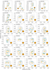 |
Fig. 1. Circular Gaussian components super-imposed on 86 GHz CLEAN images. The legend of each panel indicates the epoch at which the observations were obtained. The beam of each epoch is displayed in the panels as a filled orange circle. The contour levels correspond to 3%, 5%, 10%, 20%, 40%, and 80% of the intensity peak for all epochs, except May 2012, where 10%, 20%, 40%, and 80% of the intensity peak were used because the data quality was limited. The epochs are convolved with the same circular beam with a radius of 0.088 mas. This radius size was obtained by geometrically averaging the beam sizes of all displayed epochs. A summary of the beam parameters of each individual epoch and peak fluxes is provided in Table F.1. Each feature is labelled based on its date of emergence, with the lower number indicating an earlier ejection time. As a centre of alignment, we always used the north-westernmost feature inside the core region, which we labelled ‘C’. We note that feature ‘W2’ was detectable in the April 2002 epoch and feature ‘W6’ was not detectable in the May 2007 epoch due to S/N limitations. A summary of the characteristics of each feature is provided in Table F.5. |
Imaging with VLBI and Gaussian component model fitting can be subjective. Some alternative methods have been utilised recently, such as wavelet-based analysis (e.g. Mertens & Lobanov 2015) and CC cluster analysis techniques (e.g. Punsly et al. 2021). Inspired by the latter and in order to increase the robustness of our results, as a third step we implemented an additional CC cluster analysis, which yields very similar results, within the error budgets, for the feature identification and their velocities as computed from the Gaussian component model fitting (see Sect. 3.1). In view of uv-coverage limitations and residual calibration effects, we regard the latter method as most reliable, based on the smaller number of free fit parameters.
For the 15 and 43 GHz maps, we downloaded the respective data files (already fringe fitted and calibrated) from the websites mentioned in Sect. 2.1. We then followed the same steps as with the 86 GHz data sets. Figure 2 showcases the circular Gaussian components, super-imposed on the CC images, and the individual beam sizes and pixel scales are summarised in Table F.2 for the 43 GHz epochs. The circular Gaussian component model fitting for the 15 GHz data was exclusively done to align the images to each other, as in some epochs the C3 region (Nagai et al. 2014) was brighter than the nucleus. Cross-identifying features at this frequency with the higher frequency maps is virtually impossible, due to the large beam size at 15 GHz. The beam sizes and pixel sizes are summarised in Table F.3.
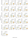 |
Fig. 2. Circular Gaussian components super-imposed on 43 GHz CLEAN images. The legend of each panel indicates the epoch at which the observations were obtained. The beam of each epoch is displayed in the bottom right side as a filled orange circle. The contour levels correspond to −1%, 1%, 2%, 4%, 8%, 16%, 32%, and 64% of the intensity peak, except in November 2010, where, due to lower data quality, the contour levels were adjusted to −10%, 10%, 20%, 40%, and 80% of the intensity peak. The epochs are convolved with the same circular beam, with a radius of 0.24 mas. This size was obtained by geometrically averaging the beam sizes of all displayed epochs. A summary of the beam parameters and peak fluxes is provided in Table F.2. Each feature is labelled based on its date of emergence, with the lower number indicating an earlier ejection time. As a centre of alignment, we always used the north-westernmost feature inside the core region, which we labelled as ‘C’. We note that feature ‘Q1’ seems to split into two (labelled ‘Q1a’ and ‘Q1b’) in August 2013; similarly, ‘Q2’ seems to split into two (labelled ‘Q2a’ and ‘Q2b’) in September 2017. These splits might be due to improved sensitivity in these epochs or variations of the intrinsic brightness and size of the jet feature or a combination of the two. A summary of the characteristics of each feature is provided in Table F.4. |
3. Analysis and results
3.1. Component cross-identification
Figures 1 and 2 showcase the travelling features over time labelled with identifiers (IDs). Our procedure for identifying a travelling feature through the epochs was as follows: starting from the 43 GHz maps, we established the trajectories of the main travelling features by requiring that the fit to their velocity produced the minimal dispersion. Continuity arguments also dictate that features cannot move upstream, barring some level of uncertainty regarding their position. A formal description of our positional error estimation is presented in Appendix F. Nevertheless, we note that some features have been reported to move back and forth (e.g. Hodgson et al. 2021), although further downstream, in the C3 region. Such a flip is interpreted as new features emerging. The model parameters are presented in Table F.4.
We established the trajectories of the core features at 86 GHz. Of course, one should expect to identify more features at 86GHz than at lower frequencies, since the generally smaller beam size resolves a finer structure near the core. A comprehensive table of the model parameters is shown in Table F.5. Five of the six 43 GHz features could be robustly cross-identified with 86 GHz features based on the matching position, time of appearance, and velocity. We labelled these features as in Table F.6. We note here, however, that our analysis implicitly assumes that the features are first visible at 86 GHz near the core and only later become visible at 43 GHz, once they have travelled further downstream. It can be argued that a scenario, in which the ejection near the core is not picked up at 86 GHz due to the sparse cadence, and is instead only later detected downstream at 43 GHz, is also possible. Finally, we point out that for the cross-identification we only focused on the positional information provided by the visibility phases and not the absolute flux information, since the flux density at 86 GHz can be subject to large uncertainties. The relative fluxes, however, are less uncertain.
In order to render the results more robust, we used the CC cluster method for estimating feature velocities as follows: first we super-resolved each image, with a beam size at least half of the nominal value presented in Tables F.1–F.3, to visually recognise each bright feature location, corresponding to a CC cluster. Then, we computed the coordinates of the CC cluster centroid by calculating the average of the CC coordinates in the image plane, inside a radius the size of the corresponding modelled Gaussian component. We used the jackknife technique (Efron & Stein 1981) to estimate the mean position. For the procedure described above, we only considered CC components with a flux above 5% of the maximum flux CC inside the radius, defined as described earlier in the section. This approach produced a second set of feature coordinates, allowing us to estimate their velocities more confidently (see Sect. 3.2) by averaging these values and the ones obtained by fitting the standard Gaussian component coordinates.
3.2. Kinematics
In Fig. 3, we show the cross-identified features. Each travelling feature is colour-coded and the open and filled symbols correspond to the 43 and 86 GHz travelling features, respectively. The dashed lines describe the velocity and (back-extrapolated) temporal point of ejection. The velocities and their uncertainties of the cross-identified features ‘F1’, ‘F2’, ‘F3’, ‘F4’, and ‘F5’ are listed next to the first time each feature is identified. They were calculated from a weighted averaging of the velocities obtained from the Gaussian component positions and from the CC cluster centroids.
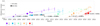 |
Fig. 3. Plot of motion of the cross-identified, colour-coded features. The empty and filled symbols correspond to the 43 and 86 GHz features, respectively. The velocity fit with the uncertainty is displayed above the first occurrence of each feature. The size of each symbol is normalised to the flux of the central feature (C) of that epoch. The velocities are also listed in Table F.6. |
Having established the feature correspondence through the years, we performed a weighted linear regression analysis to each trajectory. A formal description of the fitting procedure is presented in Appendix B. Figure 3 displays the apparent motions of the travelling features. We find that the average velocity of the 86 GHz features amounts to μWavg = 0.13 ± 0.05 mas yr−1 ( c), whereas for 43 GHz the features move, on average, at
  mas yr−1 (
 c). In order to compare the two, we also computed the 86 GHz velocity of features ejected after 2010. This calculation yields an average velocity of
  mas yr−1 (
 c) at 86 GHz4. These latter two values show a difference within their respective error budgets. Performing a z test reveals that the difference between the two values is statistically significant, to at least 2σ. Slightly larger velocities at 86 GHz may indicate that higher frequency observations trace the inner part of the jet sheath, which moves faster, whereas lower frequency 43 GHz observations detect the slower moving outer part of the sheath (see transverse velocity stratification as discussed in, e.g. Ghisellini et al. 2005). This spine-sheath scenario is more extensively discussed in Sect. 4.3.
For earlier epochs (between 1999 and 2002), we tracked the travelling features further downstream, increasing the number of data points for the fit. The feature velocities, for which an adequate number of data points for a fit were identified, are displayed in Table. F.7. Among these earlier epoch features, ‘W1’ seems to be the most intriguing. Back-extrapolating to determine the ejection year, we find that the feature emerged in 1981.63 ± 2.5, which corresponds to the onset the total intensity maximum (flare) at centimetre radio wavelengths (see Fig. 4). W1 can be tentatively identified in past maps from the literature. At 22 GHz, Venturi et al. (1993) reported a travelling feature ejection they called ‘C’5 in 1986, which can also be identified as a bright feature in the 1 mas region south-west of the nucleus, in the 43 GHz map presented in Romney et al. (1995). The position matches that of feature W1 in our 1999 86 GHz image. The trajectory of motion furthermore places W1 in the region where the diffuse blob C2 emerged (Nagai et al. 2010, 2014). We included three flux density measurements at 1 mm from the literature, denoted with green boxes in Fig. 4, to facilitate a comparison between the ejection time of W1 and the flux density peak. Although there are only three measurements available, the maximum flux at 1 mm appears roughly in 1982, consistent with the expectation that the flare first became visible at shorter wavelengths. In both cases, our analysis tentatively connects the appearance of C2 to the major outburst of early 1980s.
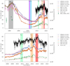 |
Fig. 4. Total variability radio light curves and γ-ray flux. Top: presented here are radio light curves of 3C 84 from 1980 to 2020 at 4.8, 8.0, 14.8, 15, 37, 230, and 345 GHz (in order of appearance in the legend). The black data points correspond to γ-ray flux. The dark-green data points are individual, historical, total flux measurements. The grey shaded area at the onset of the total intensity peak around 1983 could tentatively be connected to the ejection of feature W1, which may correspond to the prominent C2 region identified in later maps. The five other shaded areas are colour-coded in response to the cross-identified features F1 through F5, as described in Fig. 3, and denote the approximate ejection time. Bottom: zoomed-in version of the top panel showing the years 2005–2022. |
For newer epochs, the ejected features seem to move with the expected average velocity (μWavg = 0.13 ± 0.05 mas yr−1 or  c). On the other hand, features moving perpendicularly to the bulk jet flow exhibit slower speeds. A characteristic example is that of ‘W10’, which was also identified by Oh et al. (2022). The authors find a velocity of ≤0.03c, in agreement with our result of μW10 = 0.011 ± 0.011 mas yr−1 (
 c). Surprisingly, the emergence of a new feature, ‘W14’, in 2019 seems to not follow this rule. For it, we find a velocity of μW14 = 0.063 ± 0.034 mas yr−1 (
 c), close to the upper limit of ∼0.1c, which has been observed for the core region of 3C 84 in the past.
The picture becomes clearer at 43 GHz, with just six travelling features needed to describe the central region of 3C 84. Here, we make a comparison with the reported velocity range of βapp ≈ (0.086 − 0.1)c by Punsly et al. (2021). The authors of this work only used observations between August 2018 and April 2020 to study the core of 3C 84 and arrived at this result both by grouping the pair of nuclear CC and by using circular Gaussian component models. In this work, on the other hand, we did not use all available epochs in that time frame, as the goal was the direct comparison with 86 GHz images at a comparable cadence. We did, however, double the cadence for 2020 and add the more recent epochs (up to May 2021) to facilitate our analysis. In our interpretation, three features emerged in that time frame: one feature (‘Q4’), which emerged in 2018, one in early 2019 (‘Q5’), and one which emerged in early 2020 (‘Q6’). This leads to different feature velocities, with Q4 moving at μQ4 = 0.094 ± 0.007 mas yr−1 ( c) and Q6 at μQ6 = 0.093 ± 0.010 mas yr−1 (
 c). Averaging them leads to a virtually identical value of μQcomb = 0.094 ± 0.001 mas yr−1 (
 c). The feature Q5 only appears in two epochs, therefore not fulfilling our criterion set for feature velocity determination. We note here that for this comparison we used the velocity that we computed by fitting only the 43 GHz epochs.
Jorstad et al. (2017) did a similar kinematics analysis for epochs between 2007 and 2013 at 43 GHz and found moving feature velocities of βapp ∼ 0.2c further downstream (βapp = 0.5 − 3.0 mas from the VLBI core) than the region we are studying. This is in line with the known acceleration of features downstream along the jet in 3C 84 (Krichbaum et al. 1992; Dhawan et al. 1998; Suzuki et al. 2012; Punsly et al. 2021; Hodgson et al. 2021).
3.3. Outburst ejection relations
For 3C 84, a conclusive relation between radio features and γ-ray flares, as well as their ejection sites, is still elusive (see e.g. Nagai et al. 2012; Linhoff et al. 2021; Hodgson et al. 2018, 2021). The emergence of new VLBI features in AGN radio-jets (often but not always) can be associated with the onset of radio flares (e.g. Savolainen et al. 2002; Karamanavis et al. 2016). Here, we investigate the possible association between the detected new VLBI features in 3C 84 and the total intensity light curves, by back-extrapolating their trajectory to estimate the ejection time, which is the time of zero separation from the VLBI core. We also explored the connection between the flare intensity and ejected feature velocity.
Figure 4 overlays the ejection time of each feature on the radio and γ-ray light curves of 3C 84 in the top panel, with the bottom panel displaying a zoomed-in version to aid the reader in comparing the ejection times with the finer details of the variability curves. The grey shaded area in the top panel of Fig. 4 denotes the ejection time of the oldest VLBI feature we can identify in our data set, which is W1. Also, for the features F1 and F2 , only variability data at centimetre wavelength are available. The flux densities of the centimetre light curves are decaying, and no correspondence to flare activity is apparent. However, feature F3 seems to be associated with the onset of a centimetre flare peaking in 2013.19. At this time, no prominent flare in the γ-ray light curve is obvious. Feature F4 appears at the onset of a more prominent millimetre flare, which is visible in the centimetre and millimetre bands, with a peak in 2016.66. Interestingly, F4 could be associated with a γ-ray flare, which occurred at the onset of this radio flare and peaked in 2015.82. Feature F5 occurred during the decay phase of the centimetre and millimetre flare of 2016.66 and seems to correspond to a rising phase in the γ-rays, which reached the brightest γ-ray flux peak so far of 3C 84 in 2018.35. We further note that the peak of this γ-ray flare occurred after the decay of the preceding radio flare, which is quite unusual. The good correspondence of the ejection times of the features F4 and F5 with two maxima in the γ-ray light curve, which bracket this prominent centimetre and millimitre-peak, is also remarkable.
The appearance of feature F4 at the onset of the big radio flare peaking in 2016.66 and the local γ-ray flare during this ejection, suggests that the γ-ray emission region of this event is located within the VLBI core region. The relatively long time lag between the peak of the radio flux in 2016.66 and the peak of the subsequent γ-ray flare of 2018.35, however, suggests that the γ-rays of this event are produced further downstream in the jet. This hypothesis is further supported by the lack of an enhanced radio flux following this γ-ray flare. It remains unclear how the ejection of F5 relates to the observed variability in the radio bands.
Besides the individual associations between the features and the flares, there may also be one between the component velocities and the radio flux densities. The slowest feature F2 (μF2 ∼ 0.024 mas yr−1 or  ) seems to correspond to the lowest flux level out of the five features, whereas the fastest feature F4 (μF4 ∼ 0.09 mas yr−1 or
  ) corresponds to the highest flux level. The remaining features also follow this pattern (see Fig. 5). This pattern might also be transferred to the γ-ray flux, with F3, the slower out of the three overlapping features, corresponding to a lower flux level than the two remaining ones. Such behaviour could be explained if jet features move along a curved trajectory, leading to a time-variable Doppler beaming.
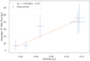 |
Fig. 5. Back-extrapolated apparent velocity of features F1 through F5 and the 37 GHz flux (S37) associated with them. A clear, increasing trend is observed. |
3.4. Image stacking
Even though image stacking smears out details from individual maps, it offers a better insight into the wider jet funnel and into its transverse profile and possible stratification. For that reason, we averaged all epochs in time at 15, 43, and 86 GHz and display them in Fig. 6. The centre of alignment was always chosen to be the core feature (labelled as C), which we defined as the north-westernmost feature in each epoch. With this choice, we eliminate effects due to time variability of the jet origin, as we can consistently align all images at the same position. We also refer to a previous core shift analysis (Paraschos et al. 2021) that shows a moderate frequency dependence of the VLBI core, typically much smaller than the beam size. The 86 GHz image showcases only the nucleus because in the southern region the diffuse flux is mostly resolved out, and thus a ridge line cannot be robustly traced. For completeness, we display the same stacked map of 3C 84 at 86 GHz in its entirety in the bottom right panel of Fig. F.1. An overview of the stacking, slicing, and Gaussian fitting procedure is detailed in Appendix C.
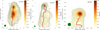 |
Fig. 6. Stacked images of 3C 84 at 15, 43, and 86 GHz. Left: 15 GHz stacked images of epochs from 2010 to 2020, as listed in Table F.3. The green disc represents the common circular beam used to convolve all images before averaging. The continuous red line depicts the ridge line, which is the point with the highest intensity at each slice. Each axis is in units of mas. The coloured region and contours correspond to regions with a S/N of at least five. Details of the beam size, flux, and rms are listed in Table F.9. The contour levels are −2%, −1%, −0.5%, 0.5%, 1%, 2%, 4%, 8%, 16%, 32%, and 64% of the intensity peak. Middle: same as left panel, but for 43 GHz. An epoch summary is listed in Table F.2. Details of the beam size, flux, and rms are listed in Table F.9. Right: same as left and middle panels, but for 86 GHz. An epoch summary is listed in Table F.1. The common convolving beam is listed in Table F.9. Details of the beam size, flux, and rms are listed in Table F.9 as well. For a zoomed-out view of the 86 GHz total intensity map at different time bins, including the 2010–2020 bin presented here, see Fig. F.1. |
3.5. Spectral index
Following the procedure described in Paraschos et al. (2021), we created spectral index maps for selected epochs (see Fig. 7), by performing a two-dimensional cross-correlation analysis. We used the optically thin and still compact emission region C3 for the alignment, except for the data from October 2020, where C3 was not well determined. Instead, we used another optically thin feature in this observation, which is located south-west of the VLBI core and is centred at (0.2, −0.4) mas. In the two earliest epochs, we identify a spectral index gradient along the north-south direction, with spectral indices from α43 − 86 ∼ 3 − 4 in the north and α43 − 86 ∼ −2 in the south. In September 2014, September 2017, and October 2020, the orientation of the spectral index gradient changed towards a northwest-southeast direction. The spectral indices range again from α43 − 86 ∼ +(2 − 4) in the northwest and α43 − 86 ∼ −2 in the southeast. Spectral indices much lower than −2 are likely due to beam resolution effects and/or uncertainties in the flux density scaling at 86 GHz and therefore may not be real. The uncertainty calculation for the individual epochs, as well as the spectral index uncertainty maps (Fig. D.1), are summarised in Appendix D.
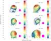 |
Fig. 7. Spectral index map of selected epochs. The contour levels were set at −1%, 1%, 2%, 4%, 8%, 16%, 32%, and 64% of the intensity peak at each epoch. The total intensity cut-off was set at 50σ. The limiting values for the spectral indices are indicated in the colour bars beside each panel. A summary of the image parameters is presented in Table F.10. The corresponding spectral index uncertainty maps are presented in Fig. D.1. |
4. Discussion
4.1. Projection effects
Our analysis presented in the previous section rests on the assumption that the jet does not significantly precess the VLBI core region and that bright VLBI features are expelled from the VLBI core region, which was identified as the most luminous feature in the radio maps. This hypothesis is physically motivated and ties well into the existing literature both for 3C 84 (see identification scheme in Nagai et al. 2014 and Oh et al. 2022), as well as for other prominent AGN jets like M 87 (Kim et al. 2018) and NGC 1052 (Baczko et al. 2016), to name only a few.
The fact that we are able to cross-identify jet components in 3C 84 at two frequencies and describe the motion of the VLBI components by a steady and linear function of time supports the assertion that we are in fact observing features ejected from the central engine. This holds for the feature trajectories from the core up to the ∼1 mas region. The limited time base of this data set does not allow us to see strong deviations from linear motion, but the misalignment between inner (sub-mas) and outer (mas-scale) VLBI jets suggests spatially bent and non-ballistical component trajectories, similar to those seen in many other AGN jets.
4.2. Jet cross-section
We used the stacked images to measure the transverse jet profile. Since the jet of 3C 84 exhibits an increasingly complex structure with increasing distance from the core (likely due to the contribution of C2 Nagai et al. 2010, 2014), we split the region of interest into two: the core region (z0 < 0.75 mas for 43 and 86 GHz observations and z0 < 1 mas for 15 GHz ones; here, z0 is the distance from the core (z0 = r|x = 0)) and the region downstream (z0 > 0.75 − 1 mas). Based on the shape of the intensity slices (see Fig. C.1), we fitted a single Gaussian function to the core region of the 86 GHz image and a double Gaussian function to the downstream region. For the 15 and 43 GHz images, we fitted a double Gaussian function in both regions. From the single Gaussian fit, we determined the full width at half maximum (FWHM) of each slice. To arrive at the deconvolved jet width, we subtracted the beam from the FWHM in quadrature. From the double Gaussian function fit, we considered the dominant (brighter) one to measure the transverse width of the main jet.
The results of our analysis are presented in Fig. 8. We find that the measured, deconvolved jet widths of the lower frequencies are overlapping close to the jet origin and the jet width becomes frequency dependent further downstream (see Fig. 8); that is, the jet width changes with frequency within core separations of 1.5 ≤ z0 ≤ 4 mas. To quantify the degree of change in jet width, we calculated the median of the differences (w15 − w43) and (w43 − w86): Δr15 − 43 = 0.091 ± 0.027 and Δr43 − 86 = 0.082 ± 0.024. The fact that the pairwise differences are both positive indicates the presence of a systematic trend. This is a characteristic property of a stratified jet, where different frequencies could map different parts of the jet (Pelletier & Roland 1989; Sol et al. 1989; Komissarov 1990). Similar limb brightening in 3C 84 was reported by Nagai et al. (2014), Giovannini et al. (2018), and Kim et al. (2019), although these studies were based only on single epochs. However, we note that the 86 GHz measurements may represent a lower limit to the true jet width; this is due to beam resolution effects and dynamic range limitations (see also Table F.9). In order to test the significance of the smaller 86 GHz jet width, we added a normally distributed random noise signal to the 15 and 43 GHz stacked images, such that their dynamic range matched that of the 86 GHz observations. Interestingly, we find that the systematic trend persists. The median values with added noise are  and
and  (i.e. still positive). This indicates that the frequency-dependent jet width may be real, even when accounting for dynamic range limitations at 86 GHz.
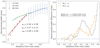 |
Fig. 8. Deconvolved jet width and jet width difference as a function of the distance from the core. Left: deconvolved jet width as a function of the distance (projected) from the VLBI core at 15, 43, and 86 GHz. The blue, green, and red markers correspond to slices taken from the 15, 43, and 86 GHz images shown in Figs. 6 and F.1, respectively. The corresponding solid lines mark the power-law fits with their indices: γ15 = 0.36 ± 0.38, γ43 = 0.27 ± 0.13, and γ86 = 0.90 ± 0.06 (see Table F.12). All slices are drawn parallel to the abscissa and are evenly spaced at 50 μas apart. We note that the 86 GHz data points might be indicating a lower limit for the jet width due to dynamic range limitations. Right: difference between the jet width at 15 GHz and 43 GHz (Δr15 − 43; dashed grey line) and 43 GHz and 86 GHz (Δr43 − 86; dashed orange line). In both cases, the median values Δr15 − 43 and Δr43 − 86 are positive. |
4.3. Jet collimation
A parameter frequently used in discriminating between jet formation models is the collimation profile; that is the width of the jet w, as a function of the distance from the core z0 (see e.g. Daly & Marscher 1988). This parameter is fundamentally tied to the characteristics of the jet and the external medium, specifically the ratio of the external pressure Pext to the internal pressure Pjet, as has been shown in theoretical models and simulations (Komissarov et al. 2007; Tchekhovskoy et al. 2008; Lyubarsky 2009). When the external pressure of the gas is described by a power law of the form P ∝ r−p, with p < 2, then the bulk jet flow follows a parabolic profile. On the other hand, if the opposite is true and p > 2, then the bulk jet flow follows a conical profile (Komissarov et al. 2009). In both cases, this pressure is counteracting the force-free expansion of the magnetised jet. In this regime, the power law from Eq. (C.3) is connected to Pext by γ = p/4.
By using a stacked image of 3C 84 (constructed from numerous epochs) to highlight the underlying structure of the jet, we attempt here, for the first time for this source, a comparison of the collimation of the jet profile of 3C 84 in the nuclear region at three different frequencies. As shown in Fig. 8, we chose to fit a power-law function to the initial expansion region where the jet width is increasing but not yet affected by the presence of C2. The resulting power-law indices are γ15 = 0.36 ± 0.38 at 15 GHz, γ43 = 0.27 ± 0.13 at 43 GHz, and γ86 = 0.90 ± 0.06 at 86 GHz, respectively. These power-law index values are summarised in Table F.12. Our result also appears to align well with the findings of Oh et al. (2022). In that work, the authors fitted both a conical and a parabolic jet profile, but they could not conclusively select one over the other. Our measurement of γ86 = 0.90 ± 0.06 at 86 GHz indicates an initially conical jet profile.
Figures 6 and F.1 showcase the complex structure of the jet of 3C 84 in the z0 > 0.75 − 1 mas region. Plotting the jet width at all three frequencies produces a jagged outline as a result of both the jet collimation and expansion (Daly & Marscher 1988), as well as image artefacts due to a low S/N at the edge of the jet. On the contrary, the difference between the jet widths at 15, 43, and 86 GHz provides a better method of investigating and illustrating whether a systematic trend is present (see Fig. 8, right). We find a decrease in jet width with increasing frequency, suggesting a transverse jet stratification scenario (i.e. spine-sheath structure; see e.g. Pelletier & Roland 1989; Sol et al. 1989; Komissarov 1990). Similar stratified jet geometries – also seen via polarisation and rotation measure analyses (e.g. O’Sullivan & Gabuzda 2009; Hovatta et al. 2012; Gabuzda et al. 2017) in other AGNs – could result from twisted magnetic flux tubes (e.g. Tchekhovskoy 2015) or hybrid models, where the central black hole and the inner accretion disc both contribute to the jet formation (Paraschos et al. 2021; Mizuno 2022).
Another possible interpretation, however, is that the observed synchrotron radiation reflects magnetised jet plasma that is undergoing rapid synchrotron cooling transverse to the jet flow. Synchrotron losses within the jet might manifest as a frequency-dependent jet width, reflecting the radial dependence of the magnetic field strength and the underlying electron power-law distribution across the jet.
A halo or cocoon enveloping the extended emission in the pc-scale region (detected at lower frequencies, e.g. Taylor & Vermeulen 1996; Silver et al. 1998; Savolainen et al. 2021) has been put forth in the past as a possible explanation of the jet collimation in 3C 84 (e.g. Nagai et al. 2017; Giovannini et al. 2018). However, this halo or cocoon is extended and exhibits a steep spectrum. Such low surface brightness temperature features are too faint to be detectable at higher frequencies with the present millimetre-VLBI array.
We note that an increased, external pressure around the nucleus of 3C 84 – for example as provided by such a cocoon or halo – would help to explain the observed downstream acceleration of moving features. In this picture, the higher external pressure on the nucleus confines the ejected features into a spatially restricted region, which the features can only traverse slowly. Further downstream, where the external pressure decreases, the features are able to accelerate more freely.
We compare the power-law indices of the jet expansion found in this work to other studies of 3C 84 from the literature. Giovannini et al. (2018) found a power-law index of γ86 ∼ 0.17, utilising RadioAstron observations of 3C 84 at 22 GHz, and Nagai et al. (2014) computed a power-law index of γ86 ∼ 0.25 using Very Long Baseline Array (VLBA) observations. Both these publications used a single epoch and took into account the entirety of the jet in their fittings. To contrast our results with these publications, we followed a similar procedure, performing a fit over the full length of the jet, which produces  at 15 GHz,
  at 43 GHz, and
  at 86 GHz, respectively. Our 43 GHz estimate of the power-law index is very similar to the one from Nagai et al. (2014) and the 22 GHz power law index by Giovannini et al. (2018) fits well into the picture of increasing power-law indices with frequency for the entirety of the southern bulk jet flow.
Collimation profile studies have also been published for several other AGNs. Boccardi et al. (2016) found that the power-law index of the collimation profile of Cygnus A is γ43 ∼ 0.55, and Hada et al. (2013) showed that for M 87 the power-law index of the collimation profile is γcombined ∼ 0.56 − 0.76. While the 86 GHz data seem to agree with these values, the lower frequency measurements are divergent. This might indicate source-dependent intrinsic differences; for example, of the jet power or in the medium that surrounds these jets (Boccardi et al. 2021).
4.4. Implications of the spectral-index values and orientation
The spectral index of a synchrotron self-absorbed emission region usually ranges between α ≤ +2.5 in the optically thick regime and −0.5 ≤ α ≤ −1 in the optically thin regime (see e.g. Rybicki & Lightman 1979). An optically thick external absorber located between the source and observer, however, could alter the spectrum, causing a stronger spectral inversion.
The highly inverted spectrum at the northern end of the 3C 84 jet (see Fig. 7) therefore suggests free-free absorption from a foreground absorber. In 3C 84, it could result, for example, from a circum-nuclear disc or torus (Walker et al. 2000). This view is further supported from recent VLBI observations at 43 GHz (KaVA) and 86 GHz (KVN), though at a lower angular resolution (Wajima et al. 2020). A foreground absorber would also act as an external Faraday screen, explaining the observed frequency-dependent polarisation in the central region (Kim et al. 2019), and it would also explain the apparent absence of the counter-jet on sub-mas scales at 86 GHz.
The observed variation in the orientation of the spectral index gradient on timescales of a few years (see Fig. 7) could challenge the interpretation via foreground absorption, unless the absorber were time variable or inhomogeneous. In any case, we have to consider the inclination of the jet relative to the observer. If we are observing the source as displayed in Fig. 14 in Kim et al. (2019), we would be peering into the bulk jet flow at an angle. The trajectories of the ejected features could be aligned or misaligned with the line of sight from time to time, thus temporarily affecting the orientation of the spectral index gradient. In this case, the variation of the orientation of the spectral index gradient in the core region could then be explained by the bent jet kinematics (helical motion, rotating jet base) rather than by some small-scale variations (sub-pc) in the foreground screen. Future monitoring observations and more detailed simulations taking into account time-dependent jet bending (helical motion) and absorber variations may shed more light on the observed variation in the spectral index gradient orientation.
5. Conclusions
In this work, we presented a detailed kinematics analysis of 3C 84 at 43 and 86 GHz. Furthermore, we established an estimate for the environment around the jet flow in the core region. Our major findings and conclusions can be summarised as follows:
-
We cross-identify moving components ejected from the VLBI core at 43 and 86 GHz. The components move with velocities of μavg = 0.04 − 0.18 mas yr−1 (
 c) on average. We find marginal evidence (∼2σ) for a faster motion at 86 GHz.
 -
The ejection of feature W1, identified at 86 GHz and possibly corresponding to C2, appears to be temporally coincident with the onset of the total intensity maximum (flare) at centimetre wavelengths in the early 1980s. For the cross-identified radio features (F1 through F5), however, a simple one-to-one correspondence between the onset of centimetre, millimetre, and γ-ray flares seems to be lacking. For components F4 and F5, the data suggest an association between component ejection and a subsequent brightening in the γ-ray band. The delayed γ-ray flare peak suggests that the region of γ-ray production is located not in the VLBI core, but further downstream.
-
The complexity of the source structure of 3C 84 complicates the measurement of the transverse jet width. However, in the innermost jet region (z0 ≤ 1 mas), we can characterise the transverse jet profile at 86 GHz by one Gaussian function. Further downstream and at 15 and 43 GHz, a double Gaussian profile is more appropriate. In this downstream region (z0 > 1.5 mas), we find evidence for a systematic variation of the jet width with frequency. From a comparison of the brighter Gaussian profile at each frequency, we formally obtain the following power-law indices for the transverse jet profiles: γ15 = 0.36 ± 0.38 at 15 GHz, γ43 = 0.27 ± 0.13 at 43 GHz, and γ86 = 0.90 ± 0.06 at 86 GHz.
-
The 86 GHz observations seem to trace the inner sheath part and suggest a parabolic jet flow profile. The 15 and 43 GHz observations, on the other hand, seem to outline the outer sheath, characterised by a more conical jet flow profile. The different profiles suggest different jet opening angles at each observed frequency or effects of synchrotron cooling transverse to the jet axis or a combination of the two.
-
The spectral index images of the individual epochs, reveal a strong spectral index gradient with a time variable orientation. Its position angle (PA) may be affected by moving jet features being ejected in different directions. Density or opacity variations in a foreground absorber, however, cannot be ruled out.
Overall, our study suggests that the jet stratification could partially explain the motion of the different features seen at 43 and 86 GHz. Currently, only a handful of VLBI observations of 3C 84 are available at intermediate frequencies (e.g. 22 GHz) and none at all at higher frequencies (e.g. 230 GHz). It is therefore important to bridge this gap by employing more and denser in-time-sampled VLBI monitoring observations in the near future. VLBI imaging at even shorter wavelengths (e.g. with the Event Horizon Telescope) will provide an even higher angular resolution, facilitating more detailed studies of the central supermassive black hole and the matter surrounding it.
We assume Λ cold dark matter cosmology with H0 = 67.8 km s−1Mpc−1, ΩΛ = 0.692, and ΩM = 0.308 (Planck Collaboration XIII 2016).
These values are obtained by computing the weighted mean of the data points, with the weights being the inverted squares of their uncertainties.
This component is different from the centre of alignment we used in our maps, also labelled C.
We considered all available epochs up to October 2020 for the 43 GHz observations, to match the time frame imposed by the 86 GHz data availability.
Acknowledgments
We thank T. Savolainen for providing software to calculate two dimensional cross-correlations. We also thank N. R. MacDonald for the proofreading and fruitful discussions which helped improve this manuscript. We thank the anonymous referee for the useful comments. G.F. P. is supported for this research by the International Max-Planck Research School (IMPRS) for Astronomy and Astrophysics at the University of Bonn and Cologne. J.-Y. K. acknowledges support from the National Research Foundation (NRF) of Korea (grant no. 2022R1C1C1005255). This research has made use of data obtained with the Global Millimeter VLBI Array (GMVA), which consists of telescopes operated by the MPIfR, IRAM, Onsala, Metsähovi, Yebes, the Korean VLBI Network, the Green Bank Observatory and the Very Long Baseline Array (VLBA). The VLBA and the GBT are a facility of the National Science Foundation operated under cooperative agreement by Associated Universities, Inc. The data were correlated at the correlator of the MPIfR in Bonn, Germany. This work makes use of 37 GHz, and 230 and 345 GHz light curves kindly provided by the Metsähovi Radio Observatory and the Submillimeter Array (SMA), respectively. The SMA is a joint project between the Smithsonian Astrophysical Observatory and the Academia Sinica Institute of Astronomy and Astrophysics and is funded by the Smithsonian Institution and the Academia Sinica. This research has made use of data from the University of Michigan Radio Astronomy Observatory which has been supported by the University of Michigan and by a series of grants from the National Science Foundation, most recently AST-0607523. This work makes use of the Swinburne University of Technology software correlator, developed as part of the Australian Major National Research Facilities Programme and operated under licence. This study makes use of 43 GHz VLBA data from the VLBA-BU Blazar Monitoring Program (VLBA-BU-BLAZAR; http://www.bu.edu/blazars/VLBAproject.html), funded by NASA through the Fermi Guest Investigator Program. This research has made use of data from the MOJAVE database that is maintained by the MOJAVE team (Lister et al. 2009b). This research has made use of the NASA/IPAC Extragalactic Database (NED), which is operated by the Jet Propulsion Laboratory, California Institute of Technology, under contract with the National Aeronautics and Space Administration. This research has also made use of NASA’s Astrophysics Data System Bibliographic Services. This research has also made use of data from the OVRO 40-m monitoring program (Richards et al. 2011), supported by private funding from the California Institute of Technology and the Max Planck Institute for Radio Astronomy, and by NASA grants NNX08AW31G, NNX11A043G, and NNX14AQ89G and NSF grants AST-0808050 and AST-1109911. S.K. acknowledges support from the European Research Council (ERC) under the European Unions Horizon 2020 research and innovation programme under grant agreement No. 771282. Finally, this research made use of the following python packages: numpy (Harris et al. 2020), scipy (Virtanen et al. 2020), matplotlib (Hunter 2007), astropy (Astropy Collaboration 2013, 2018), pandas (Pandas Development Team 2020; McKinney et al. 2010), seaborn (Waskom 2021), and Uncertainties: a Python package for calculations with uncertainties.
References
- Abdo, A. A., Ackermann, M., Ajello, M., et al. 2009, ApJ, 699, 31 [Google Scholar]
- Aleksić, J., Alvarez, E. A., Antonelli, L. A., et al. 2012, A&A, 539, L2 [NASA ADS] [CrossRef] [EDP Sciences] [Google Scholar]
- Astropy Collaboration (Robitaille, T. P., et al.) 2013, A&A, 558, A33 [NASA ADS] [CrossRef] [EDP Sciences] [Google Scholar]
- Astropy Collaboration (Price-Whelan, A. M., et al.) 2018, AJ, 156, 123 [Google Scholar]
- Atwood, W. B., Abdo, A. A., Ackermann, M., et al. 2009, ApJ, 697, 1071 [CrossRef] [Google Scholar]
- Baade, W., & Minkowski, R. 1954, ApJ, 119, 215 [NASA ADS] [CrossRef] [Google Scholar]
- Baczko, A. K., Schulz, R., Kadler, M., et al. 2016, A&A, 593, A47 [NASA ADS] [CrossRef] [EDP Sciences] [Google Scholar]
- Boccardi, B., Krichbaum, T. P., Bach, U., et al. 2016, A&A, 585, A33 [NASA ADS] [CrossRef] [EDP Sciences] [Google Scholar]
- Boccardi, B., Perucho, M., Casadio, C., et al. 2021, A&A, 647, A67 [NASA ADS] [CrossRef] [EDP Sciences] [Google Scholar]
- Britzen, S., Fendt, C., Zajaček, M., et al. 2019, Galaxies, 7, 72 [NASA ADS] [CrossRef] [Google Scholar]
- Daly, R. A., & Marscher, A. P. 1988, ApJ, 334, 539 [Google Scholar]
- Dhawan, V., Kellermann, K. I., & Romney, J. D. 1998, ApJ, 498, L111 [Google Scholar]
- Dutson, K. L., Edge, A. C., Hinton, J. A., et al. 2014, MNRAS, 442, 2048 [NASA ADS] [CrossRef] [Google Scholar]
- Efron, B., & Stein, C. 1981, Ann. Stat., 9, 586 [CrossRef] [Google Scholar]
- Fermi Large Area Telescope Collaboration 2021, ATel., 15110, 1 [Google Scholar]
- Fomalont, E. B. 1999, in Synthesis Imaging in Radio Astronomy II, eds. G. B. Taylor, C. L. Carilli, & R. A. Perley, ASP Conf. Ser., 180, 301 [Google Scholar]
- Fujita, Y., & Nagai, H. 2017, MNRAS, 465, L94 [Google Scholar]
- Gabuzda, D. C., Roche, N., Kirwan, A., et al. 2017, MNRAS, 472, 1792 [Google Scholar]
- Ghisellini, G., Tavecchio, F., & Chiaberge, M. 2005, A&A, 432, 401 [CrossRef] [EDP Sciences] [Google Scholar]
- Giovannini, G., Savolainen, T., Orienti, M., et al. 2018, Nat. Astron., 2, 472 [Google Scholar]
- Greisen, E. W. 1990, in Acquisition, Processing and Archiving of Astronomical Images, 125 [Google Scholar]
- Hada, K., Kino, M., Doi, A., et al. 2013, ApJ, 775, 70 [Google Scholar]
- Harris, C. R., Millman, K. J., van der Walt, S. J., et al. 2020, Nature, 585, 357 [NASA ADS] [CrossRef] [Google Scholar]
- Hildebrand, R. H., Whitcomb, S. E., Winston, R., et al. 1977, ApJ, 216, 698 [NASA ADS] [CrossRef] [Google Scholar]
- Ho, L. C., Filippenko, A. V., & Sargent, W. L. W. 1997, ApJS, 112, 315 [NASA ADS] [CrossRef] [Google Scholar]
- Hodgson, J. A., Rani, B., Lee, S.-S., et al. 2018, MNRAS, 475, 368 [NASA ADS] [CrossRef] [Google Scholar]
- Hodgson, J. A., Rani, B., Oh, J., et al. 2021, ApJ, 914, 43 [NASA ADS] [CrossRef] [Google Scholar]
- Homan, D. C., Ojha, R., Wardle, J. F. C., et al. 2002, ApJ, 568, 99 [NASA ADS] [CrossRef] [Google Scholar]
- Hovatta, T., Lister, M. L., Aller, M. F., et al. 2012, AJ, 144, 105 [Google Scholar]
- Hunter, J. D. 2007, Comput. Sci. Eng., 9, 90 [NASA ADS] [CrossRef] [Google Scholar]
- Jorstad, S. G., Marscher, A. P., Lister, M. L., et al. 2005, AJ, 130, 1418 [Google Scholar]
- Jorstad, S. G., Marscher, A. P., Morozova, D. A., et al. 2017, ApJ, 846, 98 [Google Scholar]
- Karamanavis, V., Fuhrmann, L., Krichbaum, T. P., et al. 2016, A&A, 586, A60 [NASA ADS] [CrossRef] [EDP Sciences] [Google Scholar]
- Kim, J. Y., Krichbaum, T. P., Lu, R. S., et al. 2018, A&A, 616, A188 [NASA ADS] [CrossRef] [EDP Sciences] [Google Scholar]
- Kim, J. Y., Krichbaum, T. P., Marscher, A. P., et al. 2019, A&A, 622, A196 [NASA ADS] [CrossRef] [EDP Sciences] [Google Scholar]
- Komissarov, S. S. 1990, Sov. Astron. Lett., 16, 284 [NASA ADS] [Google Scholar]
- Komissarov, S. S., Barkov, M. V., Vlahakis, N., & Königl, A. 2007, MNRAS, 380, 51 [Google Scholar]
- Komissarov, S. S., Vlahakis, N., Königl, A., & Barkov, M. V. 2009, MNRAS, 394, 1182 [NASA ADS] [CrossRef] [Google Scholar]
- Krichbaum, T. P., Witzel, A., Graham, D. A., et al. 1992, A&A, 260, 33 [NASA ADS] [Google Scholar]
- Landau, R., Jones, T. W., Epstein, E. E., et al. 1983, ApJ, 268, 68 [NASA ADS] [CrossRef] [Google Scholar]
- Linhoff, L., Sandrock, A., Kadler, M., Elsässer, D., & Rhode, W. 2021, MNRAS, 500, 4671 [Google Scholar]
- Lister, M. L., Cohen, M. H., Homan, D. C., et al. 2009a, AJ, 138, 1874 [NASA ADS] [CrossRef] [Google Scholar]
- Lister, M. L., Aller, H. D., Aller, M. F., et al. 2009b, AJ, 137, 3718 [Google Scholar]
- Lyubarsky, Y. 2009, ApJ, 698, 1570 [NASA ADS] [CrossRef] [Google Scholar]
- Martí-Vidal, I., Krichbaum, T. P., Marscher, A., et al. 2012, A&A, 542, A107 [NASA ADS] [CrossRef] [EDP Sciences] [Google Scholar]
- McKinney, W. 2010, in Proceedings of the 9th Python in Science Conference, eds. S. van der Walt, & J. Millman, 56 [Google Scholar]
- Mertens, F., & Lobanov, A. 2015, A&A, 574, A67 [NASA ADS] [CrossRef] [EDP Sciences] [Google Scholar]
- Mizuno, Y. 2022, Universe, 8, 85 [NASA ADS] [CrossRef] [Google Scholar]
- Nagai, H., Suzuki, K., Asada, K., et al. 2010, PASJ, 62, L11 [NASA ADS] [CrossRef] [Google Scholar]
- Nagai, H., Orienti, M., Kino, M., et al. 2012, MNRAS, 423, L122 [NASA ADS] [CrossRef] [Google Scholar]
- Nagai, H., Haga, T., Giovannini, G., et al. 2014, ApJ, 785, 53 [Google Scholar]
- Nagai, H., Chida, H., Kino, M., et al. 2016, Astron. Nachr., 337, 69 [NASA ADS] [CrossRef] [Google Scholar]
- Nagai, H., Fujita, Y., Nakamura, M., et al. 2017, ApJ, 849, 52 [NASA ADS] [CrossRef] [Google Scholar]
- Oh, J., Hodgson, J. A., Trippe, S., et al. 2022, MNRAS, 509, 1024 [Google Scholar]
- O’Sullivan, S. P., & Gabuzda, D. C. 2009, MNRAS, 400, 26 [Google Scholar]
- Pandas Development Team. 2020, https://doi.org/10.5281/zenodo.3509134 [Google Scholar]
- Paraschos, G. F., Kim, J. Y., Krichbaum, T. P., & Zensus, J. A. 2021, A&A, 650, L18 [NASA ADS] [CrossRef] [EDP Sciences] [Google Scholar]
- Pelletier, G., & Roland, J. 1989, A&A, 224, 24 [NASA ADS] [Google Scholar]
- Planck Collaboration XIII. 2016, A&A, 594, A13 [NASA ADS] [CrossRef] [EDP Sciences] [Google Scholar]
- Punsly, B. 2021, ApJ, 918, 4 [NASA ADS] [CrossRef] [Google Scholar]
- Punsly, B., Nagai, H., Savolainen, T., & Orienti, M. 2021, ApJ, 911, 19 [Google Scholar]
- Richards, J. L., Max-Moerbeck, W., Pavlidou, V., et al. 2011, ApJS, 194, 29 [Google Scholar]
- Roellig, T. L., Becklin, E. E., Impey, C. D., & Werner, M. W. 1986, ApJ, 304, 646 [NASA ADS] [CrossRef] [Google Scholar]
- Romney, J. D., Benson, J. M., Dhawan, V., et al. 1995, Proc. Nat. Academy Sci., 92, 11360 [CrossRef] [Google Scholar]
- Rybicki, G. B., & Lightman, A. P. 1979, Radiative Processes in Astrophysics (New York: Wiley) [Google Scholar]
- Savitzky, A., & Golay, M. J. E. 1964, Anal. Chem., 36, 1627 [Google Scholar]
- Savolainen, T., Wiik, K., Valtaoja, E., Jorstad, S. G., & Marscher, A. P. 2002, A&A, 394, 851 [NASA ADS] [CrossRef] [EDP Sciences] [Google Scholar]
- Savolainen, T., Giovannini, G., Kovalev, Y. Y., et al. 2021, A&A, submitted [arXiv:2111.04481] [Google Scholar]
- Scharwächter, J., McGregor, P. J., Dopita, M. A., & Beck, T. L. 2013, MNRAS, 429, 2315 [Google Scholar]
- Shepherd, M. C., Pearson, T. J., & Taylor, G. B. 1994, in Bull. Am. Astron. Soc., 26, 987 [Google Scholar]
- Silver, C. S., Taylor, G. B., & Vermeulen, R. C. 1998, ApJ, 502, 229 [NASA ADS] [CrossRef] [Google Scholar]
- Sol, H., Pelletier, G., & Asseo, E. 1989, MNRAS, 237, 411 [NASA ADS] [Google Scholar]
- Strauss, M. A., Huchra, J. P., Davis, M., et al. 1992, ApJS, 83, 29 [Google Scholar]
- Suzuki, K., Nagai, H., Kino, M., et al. 2012, ApJ, 746, 140 [Google Scholar]
- Taylor, G. B., & Vermeulen, R. C. 1996, ApJ, 457, L69 [NASA ADS] [Google Scholar]
- Tchekhovskoy, A. 2015, in The Formation and Disruption of Black Hole Jets, eds. I. Contopoulos, D. Gabuzda, & N. Kylafis, Astrophys. Space Sci. Library, 414, 45 [NASA ADS] [Google Scholar]
- Tchekhovskoy, A., McKinney, J. C., & Narayan, R. 2008, MNRAS, 388, 551 [NASA ADS] [CrossRef] [Google Scholar]
- Venturi, T., Readhead, A. C. S., Marr, J. M., & Backer, D. C. 1993, ApJ, 411, 552 [NASA ADS] [CrossRef] [Google Scholar]
- Vermeulen, R. C., Readhead, A. C. S., & Backer, D. C. 1994, ApJ, 430, L41 [Google Scholar]
- Virtanen, P., Gommers, R., Oliphant, T. E., et al. 2020, Nat. Methods, 17, 261 [Google Scholar]
- Wajima, K., Kino, M., & Kawakatu, N. 2020, ApJ, 895, 35 [Google Scholar]
- Walker, R. C., Romney, J. D., & Benson, J. M. 1994, ApJ, 430, L45 [Google Scholar]
- Walker, R. C., Dhawan, V., Romney, J. D., Kellermann, K. I., & Vermeulen, R. C. 2000, ApJ, 530, 233 [Google Scholar]
- Waskom, M. L. 2021, J. Open Source Softw., 6, 3021 [CrossRef] [Google Scholar]
- Weaver, Z. R., Jorstad, S. G., Marscher, A. P., et al. 2022, ApJS, 260, 12 [NASA ADS] [CrossRef] [Google Scholar]
Appendix A: 43 and 86 GHz contour images
Here, we briefly describe the CC images of 3C 84 at 86 and 43 GHz. They are displayed in Figs. 1 and 2, respectively. Super-imposed are circular Gaussian components used to model the flux. The features belonging to close in time epochs exhibit similar structure, which confirms our modelling. The naming convention we used is based on the observing band, plus the timestamp of the ejected feature. For example, the two features in the top left panel of Fig. 1, are labelled W2 and W1, because 86 GHz observations correspond to the W band, and W2 is upstream of W1 , and therefore it was ejected first. All described motions concern the alignment centre, which is the north-westernmost feature in the VLBI core.
Appendix B: Individual feature velocity modelling
After having identified the travelling features, we used a linear fit of the following form:
 (B.1)
(B.1)
where d(t) is the distance travelled during t, v0 is the approximately constant velocity, and d0 is the initial point of ejection, in order to estimate the velocities. Since the cross-identified features correspond to the same physical feature, we fitted a single line to both 43 and 86 GHz data points, which is displayed in Fig. 3. The fit parameters are summarised in Table F.6. Here, we implicitly assumed that position deviations due to opacity shifts are negligible. We also fitted lines to the features individually per frequency. The fit was applied to the averaged feature positions, calculated from the circular Gaussian components and the CC clusters. These individual fit parameters are summarised in Tables F.7, and F.8, as well as being displayed in Fig. B.1. We used the inverse of the uncertainties squared as weights. For our conservative uncertainty estimation, we used the approach described by Eqs. (14-5) in Fomalont (1999) for the weights, or 1/5 of the beam size (commonly used as a lower limit estimate for sufficiently high S/N images, as is the case here; see e.g. Hodgson et al. 2018; Oh et al. 2022), depending on which value was greater, for the component distance and component size uncertainties. For the P. A. errors, we used the simple error propagation of the formula θ = 2 ⋅ arctan(size/distance). All the aforementioned parameters, for all components, at both 43 and 86 GHz, are shown in Tables F.4 and F.5. With this careful approach, we incorporated systemic uncertainties, while also exceeding stochastic noise uncertainties. All parameters, describing the individual features, are summed up in Tables F.4 and F.5. The velocities together with their uncertainties derived from the fit are listed in Tables F.7 and F.8.
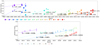 |
Fig. B.1. Plot of motion of all colour-coded features. Top: Motion of the 86 GHz features identified through all available epochs. The velocity fit with the uncertainty is displayed above the first occurrence of each feature. The size of each feature is normalised to the flux of the central feature (C) of that epoch. The velocities are also given in Table F.7. Bottom: Same as above, but for the 43 GHz features. The velocities are also given in Table F.8. |
Appendix C: Image stacking
Below, we present the image stacking and Gaussian function fitting procedure used to create Figs. 6 and 8, in detail. Since individual VLBI images can be subjective and single epochs can suffer from sidelobes and similar related imaging issues, stacking all available epochs and analysing the time-averaged image provides the highest level of confidence for our results6. Before stacking the maps, we convolved each input image with a circular Gaussian beam, the size of which was computed by averaging the major and minor axes of all input images and then calculating the geometrical beam of these averaged major and minor axes. The values of the convolving beam radii are listed in Table F.9. Since all our maps were already aligned at the origin, we need not apply any further shifts prior to averaging the images. The time-averaged maps are shown in the panels of Fig. 6, with details of the contour levels and cut-offs described in the caption. We implemented three different weighting methods to ascertain which features of the images are robust. Specifically, we applied dynamical range and rms weighting of each epoch, as well as equal weighting for all epochs. The displayed images in Fig. 6 were produced with the latter method. We find that the lower frequency flux consistently envelops the higher frequency flux.
For the jet width calculation, we made slices oriented parallel to the abscissa. We chose this approach to focus on the overall bulk jet flow and disregard individual features, which cause the ridge line to deviate locally from the overall north-south flow direction. To counteract the local deviations and better compare the mean jet widths at each frequency, we performed a Savitzky-Golay filtering (Savitzky & Golay 1964) and interpolation of the data. Here, we define the ridge line as the point of maximum intensity at each slice. The minimum distance of the first slice intersection with the ridge line to the core is dictated by the beam size: anything smaller we treat as unresolved.
To extract the jet width, for the core region at 86 GHz (z0 < 0.75 mas) we used a single Gaussian function of the following form:
 (C.1)
(C.1)
where Gtot(x) is the Gaussian function at the position x, A is the amplitude, μ is the mean value, and σ is the variance from which the FWHM of the slices transversely drawn to the bulk jet flow are calculated. For the 15 and 43 GHz observations, as well as further downstream for the 86 GHz observations, we used a sum of two Gaussian functions, Gtot = Gbright + Gfaint, and considered the FWHM of the brighter Gaussian Gbright. We calculated the deconvolved FWHM denoted as θ using the following equation:
 (C.2)
(C.2)
Figure C.1 displays the 15, 43, and 86 GHz jet profile at representative distances from the VLBI core.
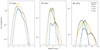 |
Fig. C.1. Representative transverse jet profiles (dots) and single and double Gaussian function fits (continuous lines) at 15, 43, and 86 GHz. Different colours represent slices in the nuclear region (z0 = 0.6 mas at 15 GHz; z0 = 0.4 mas at 43 and 86 GHz) and at separations of z0 = 1 mas, 2 mas, and 3 mas from the core, with the colour-coding as displayed in the figure legend. |
For data weighting, we used the rms from the averaged maps. The uncertainty budget of the fit δθ consists of three parts: (i) the uncertainty of the FWHM (δFWHM) of the slice for which we used the Fomalont (1999) description; (ii) the uncertainty of the fit (δfit); and (iii) an uncertainty introduced by the convolution beam (δbeam) (assumed to be 1/5 of its radius). We added them in quadrature:  .
.
We characterised the dependence of the jet width as function of core separation using a power law of the following form:
 (C.3)
(C.3)
where w(z0) is the width at distance z0 from the core, c1 is a multiplicative constant, and γ is the power-law index describing the jet expansion, with the results showcased in Fig. 8. In Table F.12, we summarise the power-law index for each frequency.
Having obtained the deconvolved bulk jet flow width, we fitted a power law of the following form:
 (C.4)
(C.4)
where w(z0) is the width at distance z0 from the core, c1 is a multiplicative constant, and γ is the power-law index describing the widening rate of the jet, with the results given in Fig. 8. The power-law index per frequency is displayed in Table F.12.
Appendix D: Spectral index uncertainty
Figure D.1 provides the spectral index uncertainty maps of the individual epochs. The uncertainty in each map can be separated into two parts: the uncertainty in the spectral index gradient P. A. and the uncertainty of the absolute values of the spectral index. The latter exists because the 86 GHz VLBI flux measurements are constantly lower than the flux measured with single-dish telescopes, as the small VLBI beam resolves out much of the diffuse flux. Thus, the flux at 86 GHz needs to be scaled up. Finally, there is some uncertainty in the registration of the phase centre of each epoch (i.e. the location of the core feature C). Paraschos et al. (2021) showed that this uncertainty is less than the pixel scale and can therefore be neglected.
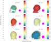 |
Fig. D.1. Individual spectral index error maps of 3C 84 between 43 and 86 GHz for the same selected epochs as in Fig. 7. The same contour levels and beam sizes were applied. A summary of the image parameters is presented in Table F.10. The procedure to determine the uncertainties is described in Appendix D. |
We followed the procedure described in the appendix of Kim et al. (2019) to find the scaling factor g and its uncertainty δg per epoch. The spectral index is defined as
 (D.1)
(D.1)
where (ν43, S43) and (ν86, S86) are the frequency and flux at 43 and 86 GHz, respectively. We then calculated the spectral index uncertainty through standard error propagation, taking into account the uncertainties from the fluxes (δS43, and δS86) and from the scaling factor (δg). The resulting maps exhibit values between α43 − 86 ∼ 0.1 − 0.7, except for the May 2014 and September 2014 observations, where the uncertainty rises to α43 − 86 ∼ 1.0 − 1.2.
For the estimation of the robustness of the P. A. of the spectral index gradient to the change from north-south to northwest-southeast, we shifted the October 2020 map in both x and y axes and studied the directionality of the spectral index gradient. In the currently displayed image, the P. A. of the shift between the 43 and 86 GHz image is P.A. = ∼68°. We found that in order to produce a north-south-oriented spectral index, we needed to shift the same two images by P.A. = ∼21°, which is a significant offset. We can thus conclude, that the orientation of the spectral index gradient is robust.
Appendix E: Time binning
Figure F.1 displays two different time binning methods of the epochs presented in Fig. 1. The top four panels show a six-year bin, whereas the bottom two ones show an approximately ten-year bin. In the six-year binned images, we can recognise the swinging of the P. A. of the southern jet. In the first bin, the bulk of the jet flow follow a southwest trajectory. In the second bin, we find a purely southern flow. The third bin is less conclusive, although a tendency towards a southeast trajectory can be recognised, which is then confirmed in the last bin. We can conclude that the period swing is approximately six years, which agrees well with the estimate of five to ten years found by Punsly et al. (2021). On the other hand, in the ten year bin, this behaviour is less pronounced. One conclusion we can draw from the ten-year time bins is that the jet has expanded towards the south, from ∼1.5 mas to ∼3.5 mas.
Zooming in on the core region in Fig. F.1, the east-west elongation seems absent in the first time bin and can only be tentatively detected in second time bin. Then, it features more prominently in the third and fourth bins. Moving further south to the 0.5 − 1.5 mas region, the jet seems ridge brightened, before turning limb brightened in the mid 2000s. This is in line with the previous work by other authors at lower frequencies (e.g. Walker et al. 2000; Nagai et al. 2014 at 22 and 43 GHz).
Appendix F: Parameter tables
In this section, we present all the tables mentioned in the main text. Table F.1 displays the 86 GHz epoch, synthesised beam size of the array, pixel scale of the images created, as well as the total intensity maximum in Jy/beam. Accordingly, Table F.2 and Table F.3 refer to the same parameters for the 43 and 15 GHz epochs. Homan et al. (2002) estimated a flux uncertainty of the order of 5% to 10% for individual features in 22 GHz images, and Punsly (2021) estimated 10% for 43 GHz images. Our approach is to be conservative with our error estimation; therefore, we factor in a 20% uncertainty for all our epochs at each frequency. It should be noted here that the GMVA is known to suffer from large uncertainties in the flux density. A visibility scaling method is introduced by Kim et al. (2019), culminating in an up-scaling factor of the order two. Our analysis is independent of the absolute flux densities, and thus we opted not to apply this correction. The reader should therefore keep in mind that the various GMVA fluxes reported in this study might we underestimated by a factor of ∼2.
Summary of image parameters at 86 GHz.
Summary of image parameters at 43 GHz.
Summary of image parameters at 15 GHz.
Tables F.4 and F.5 summarise all the moving features we identified at 86 and 43 GHz, respectively. The first column denotes the individual feature ID. The second column is the observing epoch; column three denotes the flux of the fit feature. The final three columns correspond in sequence to the distance and the P. A. between each feature and the core, and the size of the feature, defined as the width of the feature.
Physical parameters of each model feature at 43 GHz.
Physical parameters of each model feature at 86 GHz.
Table F.6 contains a list of the IDs and velocities of the cross-identified features. For these cross-identified features, we estimate the error for the ejection year to be ±6 months, which is set by the average cadence of available 86 GHz epochs. Tables F.7 and F.8 display the feature IDs and corresponding interpolated velocity at 86 and 43 GHz, respectively. Components ‘W4’, ‘W5’, and ‘W13’ were only identified in one epoch and we therefore could not derive a velocity estimate. For the individual features, we impose a 5σ uncertainty (with 1σ = 0.5 years, from the cross-identified features), and thus conservatively estimate the error for the ejection year to be ±2.5 years. A description of the fitting method and error estimation is offered in Appendix B.
Combined feature velocity and ejection date of cross-identified features.
Component velocity and ejection date at 86 GHz.
Component velocity and ejection date at 43 GHz.
Table F.9 displays the circular convolving beam used to produce the stacked images of Fig. 6, per frequency. The last two columns correspond to the intensity peak of the stacked image and the rms error. Similarly, Table F.11 displays the parameters associated with Fig. F.1.
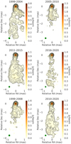 |
Fig. F.1. Full showcase of stacked images of 3C 84 at 86 GHz, with different time bins. The title of each panel indicates the time bin used. The same procedure was followed to produce the panels, as described in the caption of Fig. 6. All image parameters are summarised in Table F.11 |
Summary of image parameters for the stacked images.
Summary of image parameters of the spectral index maps.
Summary of image parameters of the time binned stacked images.
Finally, Table F.12 displays the power-law indices per frequency. The fitting procedure and error estimation is explained in Appendix C.
Power-law fit parameters for the stacked images per frequency.
All Tables
All Figures
|
Fig. 1. Circular Gaussian components super-imposed on 86 GHz CLEAN images. The legend of each panel indicates the epoch at which the observations were obtained. The beam of each epoch is displayed in the panels as a filled orange circle. The contour levels correspond to 3%, 5%, 10%, 20%, 40%, and 80% of the intensity peak for all epochs, except May 2012, where 10%, 20%, 40%, and 80% of the intensity peak were used because the data quality was limited. The epochs are convolved with the same circular beam with a radius of 0.088 mas. This radius size was obtained by geometrically averaging the beam sizes of all displayed epochs. A summary of the beam parameters of each individual epoch and peak fluxes is provided in Table F.1. Each feature is labelled based on its date of emergence, with the lower number indicating an earlier ejection time. As a centre of alignment, we always used the north-westernmost feature inside the core region, which we labelled ‘C’. We note that feature ‘W2’ was detectable in the April 2002 epoch and feature ‘W6’ was not detectable in the May 2007 epoch due to S/N limitations. A summary of the characteristics of each feature is provided in Table F.5. |
| In the text | |
|
Fig. 2. Circular Gaussian components super-imposed on 43 GHz CLEAN images. The legend of each panel indicates the epoch at which the observations were obtained. The beam of each epoch is displayed in the bottom right side as a filled orange circle. The contour levels correspond to −1%, 1%, 2%, 4%, 8%, 16%, 32%, and 64% of the intensity peak, except in November 2010, where, due to lower data quality, the contour levels were adjusted to −10%, 10%, 20%, 40%, and 80% of the intensity peak. The epochs are convolved with the same circular beam, with a radius of 0.24 mas. This size was obtained by geometrically averaging the beam sizes of all displayed epochs. A summary of the beam parameters and peak fluxes is provided in Table F.2. Each feature is labelled based on its date of emergence, with the lower number indicating an earlier ejection time. As a centre of alignment, we always used the north-westernmost feature inside the core region, which we labelled as ‘C’. We note that feature ‘Q1’ seems to split into two (labelled ‘Q1a’ and ‘Q1b’) in August 2013; similarly, ‘Q2’ seems to split into two (labelled ‘Q2a’ and ‘Q2b’) in September 2017. These splits might be due to improved sensitivity in these epochs or variations of the intrinsic brightness and size of the jet feature or a combination of the two. A summary of the characteristics of each feature is provided in Table F.4. |
| In the text | |
|
Fig. 3. Plot of motion of the cross-identified, colour-coded features. The empty and filled symbols correspond to the 43 and 86 GHz features, respectively. The velocity fit with the uncertainty is displayed above the first occurrence of each feature. The size of each symbol is normalised to the flux of the central feature (C) of that epoch. The velocities are also listed in Table F.6. |
| In the text | |
|
Fig. 4. Total variability radio light curves and γ-ray flux. Top: presented here are radio light curves of 3C 84 from 1980 to 2020 at 4.8, 8.0, 14.8, 15, 37, 230, and 345 GHz (in order of appearance in the legend). The black data points correspond to γ-ray flux. The dark-green data points are individual, historical, total flux measurements. The grey shaded area at the onset of the total intensity peak around 1983 could tentatively be connected to the ejection of feature W1, which may correspond to the prominent C2 region identified in later maps. The five other shaded areas are colour-coded in response to the cross-identified features F1 through F5, as described in Fig. 3, and denote the approximate ejection time. Bottom: zoomed-in version of the top panel showing the years 2005–2022. |
| In the text | |
|
Fig. 5. Back-extrapolated apparent velocity of features F1 through F5 and the 37 GHz flux (S37) associated with them. A clear, increasing trend is observed. |
| In the text | |
|
Fig. 6. Stacked images of 3C 84 at 15, 43, and 86 GHz. Left: 15 GHz stacked images of epochs from 2010 to 2020, as listed in Table F.3. The green disc represents the common circular beam used to convolve all images before averaging. The continuous red line depicts the ridge line, which is the point with the highest intensity at each slice. Each axis is in units of mas. The coloured region and contours correspond to regions with a S/N of at least five. Details of the beam size, flux, and rms are listed in Table F.9. The contour levels are −2%, −1%, −0.5%, 0.5%, 1%, 2%, 4%, 8%, 16%, 32%, and 64% of the intensity peak. Middle: same as left panel, but for 43 GHz. An epoch summary is listed in Table F.2. Details of the beam size, flux, and rms are listed in Table F.9. Right: same as left and middle panels, but for 86 GHz. An epoch summary is listed in Table F.1. The common convolving beam is listed in Table F.9. Details of the beam size, flux, and rms are listed in Table F.9 as well. For a zoomed-out view of the 86 GHz total intensity map at different time bins, including the 2010–2020 bin presented here, see Fig. F.1. |
| In the text | |
|
Fig. 7. Spectral index map of selected epochs. The contour levels were set at −1%, 1%, 2%, 4%, 8%, 16%, 32%, and 64% of the intensity peak at each epoch. The total intensity cut-off was set at 50σ. The limiting values for the spectral indices are indicated in the colour bars beside each panel. A summary of the image parameters is presented in Table F.10. The corresponding spectral index uncertainty maps are presented in Fig. D.1. |
| In the text | |
|
Fig. 8. Deconvolved jet width and jet width difference as a function of the distance from the core. Left: deconvolved jet width as a function of the distance (projected) from the VLBI core at 15, 43, and 86 GHz. The blue, green, and red markers correspond to slices taken from the 15, 43, and 86 GHz images shown in Figs. 6 and F.1, respectively. The corresponding solid lines mark the power-law fits with their indices: γ15 = 0.36 ± 0.38, γ43 = 0.27 ± 0.13, and γ86 = 0.90 ± 0.06 (see Table F.12). All slices are drawn parallel to the abscissa and are evenly spaced at 50 μas apart. We note that the 86 GHz data points might be indicating a lower limit for the jet width due to dynamic range limitations. Right: difference between the jet width at 15 GHz and 43 GHz (Δr15 − 43; dashed grey line) and 43 GHz and 86 GHz (Δr43 − 86; dashed orange line). In both cases, the median values Δr15 − 43 and Δr43 − 86 are positive. |
| In the text | |
|
Fig. B.1. Plot of motion of all colour-coded features. Top: Motion of the 86 GHz features identified through all available epochs. The velocity fit with the uncertainty is displayed above the first occurrence of each feature. The size of each feature is normalised to the flux of the central feature (C) of that epoch. The velocities are also given in Table F.7. Bottom: Same as above, but for the 43 GHz features. The velocities are also given in Table F.8. |
| In the text | |
|
Fig. C.1. Representative transverse jet profiles (dots) and single and double Gaussian function fits (continuous lines) at 15, 43, and 86 GHz. Different colours represent slices in the nuclear region (z0 = 0.6 mas at 15 GHz; z0 = 0.4 mas at 43 and 86 GHz) and at separations of z0 = 1 mas, 2 mas, and 3 mas from the core, with the colour-coding as displayed in the figure legend. |
| In the text | |
|
Fig. D.1. Individual spectral index error maps of 3C 84 between 43 and 86 GHz for the same selected epochs as in Fig. 7. The same contour levels and beam sizes were applied. A summary of the image parameters is presented in Table F.10. The procedure to determine the uncertainties is described in Appendix D. |
| In the text | |
|
Fig. F.1. Full showcase of stacked images of 3C 84 at 86 GHz, with different time bins. The title of each panel indicates the time bin used. The same procedure was followed to produce the panels, as described in the caption of Fig. 6. All image parameters are summarised in Table F.11 |
| In the text | |
Current usage metrics show cumulative count of Article Views (full-text article views including HTML views, PDF and ePub downloads, according to the available data) and Abstracts Views on Vision4Press platform.
Data correspond to usage on the plateform after 2015. The current usage metrics is available 48-96 hours after online publication and is updated daily on week days.
Initial download of the metrics may take a while.