| Issue |
A&A
Volume 659, March 2022
|
|
|---|---|---|
| Article Number | A194 | |
| Number of page(s) | 14 | |
| Section | Astrophysical processes | |
| DOI | https://doi.org/10.1051/0004-6361/202141375 | |
| Published online | 28 March 2022 | |
A unified accretion-ejection paradigm for black hole X-ray binaries
VI. Radiative efficiency and radio–X-ray correlation during four outbursts from GX 339-4
1
Institute of Astronomy, University of Cambridge, Madingley Road, Cambridge CB3 OHA, UK
2
Villanova University, Department of Physics, Villanova, PA 19085, USA
e-mail: This email address is being protected from spambots. You need JavaScript enabled to view it.
or This email address is being protected from spambots. You need JavaScript enabled to view it.
3
Univ. Grenoble Alpes, CNRS, IPAG, 38000 Grenoble, France
4
IRAP, Université de Toulouse, CNRS, UPS, CNES, Toulouse, France
5
Universitá degli Studi di Palermo, Dipartimento di Fisica e Chimica, Via Archirafi 36, 90123 Palermo, Italy
6
INAF/IASF Palermo, Via Ugo La Malfa 153, 90146 Palermo, Italy
7
AIM, CEA, CNRS, Université Paris-Saclay, Université Paris Diderot, Sorbonne Paris Cité, 91191 Gif-sur-Yvette, France
8
Station de Radioastronomie de Nançay, Observatoire de Paris, PSL Research University, CNRS, Univ. Orléans, 18330 Nançay, France
Received:
24
May
2021
Accepted:
27
September
2021
Abstract
The spectral evolution of transient X-ray binaries can be reproduced by an interplay between two flows separated at a transition radius RJ: a standard accretion disk (SAD) in the outer parts beyond RJ and a jet-emitting disk (JED) in the inner parts. In the previous papers in this series we successfully recover the spectral evolution in both X-rays and radio for four outbursts of GX 339-4 by playing independently with the two parameters: RJ and the disk accretion rate Ṁin. In this paper we compare the temporal evolution of both RJ and Ṁin for the four outbursts. We show that despite the undeniable differences between the time evolution of each outburst, a unique pattern in the Ṁin−RJ plane seems to be followed by all cycles within the JED-SAD model. We call this pattern a fingerprint, and show that even the “failed” outburst considered follows it. We also compute the radiative efficiency in X-rays during the cycles and consider its impact on the radio–X-ray correlation. Within the JED-SAD paradigm, we find that the accretion flow is always radiatively efficient in the hard states, with between 15% and 40% of the accretion power being radiated away at any given time. Moreover, we show that the radiative efficiency evolves with the accretion rate because of key changes in the JED thermal structure. These changes give birth to two different regimes with different radiative efficiencies: the thick disk and the slim disk. While the existence of these two regimes is intrinsically linked to the JED-SAD model, we show direct observational evidence of the presence of two different regimes using the evolution of the X-ray power-law spectral index, a model-independent estimate. We then argue that these two regimes could be the origin of the gap in X-ray luminosity in the hard state, the wiggles, and different slopes seen in the radio–X-ray correlation, and even the existence of outliers.
Key words: accretion, accretion disks / black hole physics / magnetohydrodynamics (MHD) / ISM: jets and outflows / X-rays: binaries
© ESO 2022
1. Introduction
Black hole X-ray binaries are composed of a stellar mass black hole and a companion star. Over time, matter from the companion accretes onto the black hole to form an accretion flow or accretion disk (for a review, see Remillard & McClintock 2006). While X-ray binaries spend most of their life in a quiescent and barely detectable state, they often undergo huge outbursts usually detected in X-ray (Dunn et al. 2010). All sources have different behaviors; some undergo outbursts every other year, while others have been stuck in outburst since their discovery (see Tetarenko et al. 2016). Each outburst from a given source is unique, but most follow a similar evolution through two distinct spectral states observed in X-rays: hard and soft. The hard state is characterized by a Comptonization spectrum mainly in the hard X-rays (above 10 keV), while the soft state is characterized by a disk blackbody with typical temperature in the soft X-rays (below 1 keV). During a given outburst, a source will start in the quiescent state and rise in luminosity in the hard state for up to 3−4 orders of magnitude (see, however, failed outbursts; Tetarenko et al. 2016, and references therein). Once it reaches Eddington-like luminosities in X-ray ≳10% LEdd the source transitions to the soft state, where luminosity will gradually decrease. When the luminosity reaches about 1−5% LEdd, a luminosity that seems constant for all outbursts from a given source (Maccarone 2003), the source transitions back to the hard state where it will eventually return to the quiescent state. In this common behavior, transition phases between hard and soft usually last a few days, while both the hard and the soft phases can last months. In addition to these changes in X-ray, we observe drastic variations at other wavelengths, especially in radio bands. During the hard state, a weak radio counterpart is usually detected. However, it disappears (is quenched) entirely when the system reaches the soft state. A key correlation has been discovered in the hard state between the radio (around 5−9 GHz) and the soft X-rays (usually 1−10 keV or 3−9 keV; Hannikainen et al. 1998; Corbel et al. 2003; Gallo et al. 2003). There are two major tracks in this correlation, labeled standard and outliers for historical reasons, and their origin is still unknown (Gallo et al. 2012, 2018; Corbel et al. 2013; Huang et al. 2014), although possible differences in the jets (Espinasse & Fender 2018) or the accretion flow properties have been mentioned (Coriat et al. 2011; Koljonen & Russell 2019). In addition to these two jets, strong winds are usually detected, especially in the soft states (see, e.g., Ponti et al. 2012). However, it is still unclear exactly when these winds are produced and observed (see introduction in Petrucci et al. 2021).
The behavior depicted above is quite generic and well characterized, but there is still no consensus explanation about what causes a cycle and what drives the evolution in X-rays and radio (Done et al. 2007; Yuan & Narayan 2014). A unified framework, the jet-emitting disk–standard accretion disk (JED-SAD) paradigm has been progressively developed to address these points in a series of papers. The framework was proposed by Ferreira et al. (2006, hereafter Paper I). They assume that the accretion disk is threaded by a large-scale magnetic field, whose radial distribution separates the disk into two different accretion flows. Outside a radius RJ, in the outer region, the disk is barely magnetized, in the regime that they call a standard accretion disk (SAD, Shakura & Sunyaev 1973). In this regime, accretion is mainly due to turbulence, through what we now think is the magneto-rotational instability (MRI, Balbus & Hawley 1991; Balbus 2003). Although ejections (winds or jets) can be produced in these conditions, they have been neglected in this paradigm so far, as we assume that only the inner region produces ejections (see Fig. 1 and below). In its inner region, from the inner-most stable circular orbit (ISCO) Risco to the transition radius RJ, the disk is magnetized around equipartition (i.e., the magnetic pressure is approximately the sum of the radiative and gaseous pressures). The presence of a strong vertical magnetic field allows for the production of powerful and self-confined ejections (Blandford & Payne 1982), and these ejections apply a torque on the disk that accelerates matter. This regime is called a jet-emitting disk (JED, Ferreira & Pelletier 1993a,b, 1995). We show an example of JED-SAD configuration in Fig. 1, adapted from Marcel et al. (2018a). We invite the interested reader to study the previous papers in this series (see next paragraph), the seminal papers of the JEDs (Ferreira & Pelletier 1993a,b, 1995), as well as the latest numerical calculations (Jacquemin-Ide et al. 2019, 2021) and related simulations (Scepi et al. 2019; Liska et al. 2019).
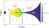 |
Fig. 1. Example of solution showing the geometry of the JED-SAD paradigm. From left to right: black hole (in black), jet-emitting disk from Risco to RJ (in yellow–green), and standard accretion disk beyond RJ (violet). This example is an actual physical calculation, where the color is the actual electron temperature, adapted from Fig. 1 in Marcel et al. (2018a). |
In order to compare this framework to observations, Marcel et al. (2018b, hereafter Paper II) designed a two-temperature plasma code that computes the thermal structure and its associated spectral emission for a JED (i.e., RJ is pushed to infinity in Fig. 1). They showed that a JED could be the source of the hard X-rays (i.e., the region commonly called corona) in a given set of parameters. These parameters are either linked to the micro-physics or global parameters such as the black hole spin or mass, or even the distance to the source. The parameter set was chosen to be physically consistent with numerical calculations (Jacquemin-Ide et al. 2019, 2021), observations (Petrucci et al. 2010), and the known parameters of the source GX 339-4 (Marcel et al. 2018b). They then added an outer standard accretion disk (SAD) outside of the radius RJ (see Fig. 1 and Marcel et al. 2018a, hereafter Paper III), essentially making RJ a parameter in the model. They froze all the parameters in the model to their expected value from Paper II, and showed that the canonical states observed in X-ray binaries could be reproduced by playing independently with only two remaining parameters: the transition radius RJ and the accretion rate in the disk Ṁin. It is important to note here that the model does not need nor does it include any normalization. The X-ray flux is directly dependant on the thermal state of the disk (e.g., temperature, density, optical depth) as well as the distance to the source. Later, they qualitatively reproduced four full cycles of GX 339-4, playing again only with RJ and Ṁ (Marcel et al. 2019, Paper IV; Marcel et al. 2020, Paper V). Their spectral fitting method (see Sect. 2.1) includes both radio and X-rays, and compared the results to the presence of quasi-periodic oscillations. We invite the reader to read the previous papers in the series for more detailed discussions about the theoretical framework (Paper I), other models (Paper II, Introduction), the assumptions and equations resolved (Papers II, III), the fitting procedure and the inclusion of radio flux (Paper IV), and the comparison to timing properties (Paper V).
The goal of the present study is to build up a generic picture of the archetypal source GX 339-4 within the JED-SAD paradigm. We then use this generic picture and tackle questions about the radiative efficiency of the accretion flow and the radio–X-ray correlation. In Sect. 2 we describe the methodology used, and show that all four outbursts from GX 339-4 follow a similar path in the theoretical Ṁin−RJ plane despite clear differences between outbursts. In Sect. 3 we focus on the evolution of the disk structure within the JED-SAD paradigm, and we address the existence of two different accretion regimes during the hard state. We then discuss the evolution of the radiative efficiency of the accretion flow in Sect. 4, as well as possible observational evidence for these different regimes. We also discuss the impact on the radio–X-ray correlation. We detail the important possible caveats in Sect. 5, before discussing and concluding in Sect. 6.
2. A unique fingerprint for GX 339-4
2.1. Methodology
The hybrid disk configuration is composed of a black hole of mass M, an inner jet-emitting disk (JED) from the inner stable circular orbit Risco to the transition radius RJ, and an outer standard accretion disk (SAD) from RJ to Rout. The system is assumed to be at a distance D from the observer. In the following we adopt the dimensionless scalings r = R/Rg, where Rg = GM/c2 is the gravitational radius; m = M/M⊙; and the local disk accretion rate ṁ = Ṁ/ṀEdd, where ṀEdd = LEdd/c2 is the Eddington accretion rate and LEdd is the Eddington luminosity (Eddington 1926). Because jets carry matter away from the disk, the accretion rate in a JED varies with radius ṁ ∝ rξ (Ferreira & Pelletier 1995; Blandford & Begelman 1999), where the ejection efficiency ξ is sometimes labeled p or s to avoid confusion with the ionization parameter. We use ξ = 0.01 in our analysis, consistent with the work from previous papers in this series and the most recent self-similar calculations on the issue (see, e.g., Jacquemin-Ide et al. 2019, Fig. 7). We also mainly refer to the accretion rate at the ISCO, ṁin, leading to ṁ(r) = ṁin (r/risco)ξ at any given radius r ≤ rJ in the JED, and ṁ(r) = ṁin(rJ/risco)ξ at any given radius r ≥ rJ in the SAD. In practice the accretion rate is almost constant since we use ξ ≪ 1. Since we focus on the archetypal object GX 339-4, we use a black hole mass m = 5.8, a spin a = 0.93 corresponding to risco = 2.0, and a distance D = 8 kpc (Miller et al. 2004; Muñoz-Darias et al. 2008; Parker et al. 2016; Heida et al. 2017, for more recent estimates). The impact of the different parameters (e.g., ξ, ms, risco) is thoroughly discussed in the previous papers in the series.
Four outbursts of GX 339-4, from 2002 to 2011, were successfully recovered by playing with only the two (assumed) independent parameters rJ and ṁin. Each observation consists in a 3−25 keV X-ray spectral energy distribution (RXTE/PCA) that we compare to our global theoretical spectral energy distribution. Some observations are also accompanied by a radio flux density at 8.6 or 9 GHz (ATCA) that we compare to our radio flux estimate using
 (1)
(1)
with f̃R the normalization factor (Paper IV). For each observation, we find the parameter pair (rJ,ṁin)(t) that best reproduces the main X-ray spectral parameters and the radio flux (when observed within one day of the X-ray). We refer the reader to the previous papers in this series for further details on the spectral parameters chosen, the fitting method, and the radio estimates (Sect. 3 in Paper IV), as well as the spectral coverage in radio and X-rays (Figs. 1–3 in Paper V).
2.2. Temporal evolution
We show in Fig. 2 the evolution of rJ(t) and ṁin(t), along with their 5% confidence regions for the four different outbursts from left to right: 2002–2003 (#1), 2004–2005 (#2), 2006–2007 (#3), and 2010–2011 (#4). These confidence regions describe the intervals for rJ and ṁin, where any variation will lead to a change of at most 5% in the best fit. In Paper IV, especially Sect. 3.2.1, we discuss these error bars and their importance. We use a unique color-scale for each outburst to show its unique time-evolution: an outburst starts in dark violet during the rising hard state and finishes in light yellow in the decaying hard state. We use a classical definition of the spectral states: quiescent, hard, hard- and soft-intermediate, and soft states (see Paper IV for their precise definitions). For ease of comparison between the various outbursts, we define five labels: A, B, C, D, and E, similarly to what was done by Petrucci et al. (2008) and Kylafis & Belloni (2015). We define Point A as the quiescent state, not visible in Fig. 2. We define Point B as the last hard state of the rising phase, C and D as the first and last soft states, and E as the first hard state of the decaying phase. While the position of each label depends on the arbitrary definition chosen for each state (i.e., hard, hard-intermediate, soft-intermediate, or soft) they are convenient to help follow a given outburst.
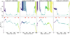 |
Fig. 2. Evolution along time of rJ (top) and ṁin (bottom) for all four outbursts of GX 339-4 observed by RXTE with their 5% confidence regions. For each outburst the timescale is chosen so that t = 0 corresponds to the first detection of the outburst (see Paper V for more details). The color-coding translates the time evolution for each outburst: starting in dark violet during the rising hard state and finishing in light yellow in the decaying hard state, using a constant color during the entire soft and soft-intermediate states. Four letters are placed to guide the evolution of each outburst: Point B is the last hard state of the rising phase, C and D are the first and last soft states, and E is the first hard state of the decaying phase. |
In our paradigm, each outburst undergoes the following steps: a rise in ṁin in the hard-state until B, a decrease in rJ in the transition to the soft-state where rJ reaches the ISCO until C, a gradual decrease in ṁin in the soft-state where rJ stays at the ISCO until D, an increase in rJ to come back to the hard-state until E, and a decrease in ṁin to go back to quiescence. In Fig. 2 the two parameters (rJṁin) seem to vary independently: rJ undergoes its swiftest variations while ṁin remains constant, and vise versa. This typical behavior is especially visible in outburst #4, where variations are much clearer and smoother thanks to smaller confidence regions due to the presence of radio flux in the fits. This is the behavior expected in the qualitative picture proposed in Paper I, but also in Esin et al. (1997), although these authors make different assumptions and do not take into account the effect of jets on the accretion flow dynamics. We note that there are a few alternative scenarios trying to explain state transitions using either evaporation processes (Meyer & Meyer-Hofmeister 1994; Meyer-Hofmeister et al. 2005), a disk dynamo (Begelman & Armitage 2014), or the cosmic battery (Kylafis & Belloni 2015).
While all outbursts follow the same generic evolution (A-B-C-D-E-A), the paths followed by rJ(t) and ṁin(t) are actually disparate. One important difference is the duration of each spectral state phase, as visible in Fig. 2. Transitions between hard and soft states ([B, C] and [D, E]) typically last 15–50 days, whereas other phases can last up to hundreds of days. This is even more visible when focusing on outbursts #1 and #3, for example. While [B, C] and [D, E] form two different pairs separated by 200 days in outburst #1, all four steps are within a 100-day period in outburst #3. These two outbursts are thus very different in their temporal evolutions, and there seems to be no generic behavior.
2.3. From the HID to the ṁin − rJ plane
One usually assumes that the main parameter controlling the outbursts is the disk accretion rate (Esin et al. 1997). It is therefore practical to represent each observational point in a theoretical (parametric) plane: rJ as function of ṁin. This is done in Fig. 3 using the same color-coding and labels (B, C, D, E) as in Fig. 2. Each outburst starts in the dark violet phase, follows a path going through points B, C, D, and E, and then finishes in the light yellow phase. These 2D figures are thus physical analogs of the hardness-intensity diagram. Two main comments can be drawn from these figures. First, while the time evolution rJ(t) and ṁin(t) of outbursts #1 and #3 were incompatible (see Sect. 2.2), the paths followed in the ṁin−rJ plane show impressive similarities, as illustrated by the similar position of the labels. Second, the pattern drawn in the ṁin−rJ plane is clearer for outburst #4 than for the other three. There are two reasons for this. Incidentally, the low-luminosity rising hard phase was not observed, which prevents the rising (dark violet) and decaying (light yellow) phases from obscuring each other. More importantly, the confidence regions of rJ and ṁin in outburst #4 are much smaller in the hard state due to the excellent radio coverage of both the rising and decaying phases (see Paper V). This advocates for the systematic use of radio constraints to derive the physical state of the disk.
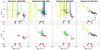 |
Fig. 3. Positions of each observation in the ṁin−rJ plane for each outburst: all observations (top), only those when radio constraints are present (bottom). The colors are the same as in Fig. 2: each outburst starts in the dark violet phase, transitions to the soft state in green, and comes back to the hard state in the light yellow phase. Additionally, the labels B–E from Fig. 2 are shown. |
We display in the bottom panels of Fig. 3 the observations for which the radio flux was used to better constrain the fits. All fitting points with huge error bars are now disregarded. For outburst #1 we are only left with the last steps of the rising hard state (dark violet) and the very end of the decaying hard state (light yellow). For outbursts #2 and #4, the rising and decaying phases are both still visible. For outburst #3 a few points at the end of the rising phase and most of the decaying phase are still present. Nevertheless, the track drawn in the ṁin−rJ plane now appears much clearer in the hard state branch, with the least certain fits being ignored. The main striking point of this representation in the ṁin−rJ plane, where timescales are discarded, is the hint of the existence of a common pattern for GX 339-4 (see labels B, C, D, and E). This is discussed further below.
2.4. A characteristic pattern in the ṁin − rJ plane
We display in light gray in Fig. 4 all observations in the ṁin−rJ plane for the four full outbursts. Here “constrained observations” are all observations except those in the hard state with no simultaneous radio coverage (see Sect. 2.3). They represent 852 observations out of the total of 1036 spread over the four full outbursts, and we show them in Fig. 4 using the same color-coding as in Figs. 2 and 3. For completeness, the constrained observations from the 2008–2009 failed outburst from GX 339-4 (see Fig. 1 in Marcel et al. 2020) are also shown in pink.
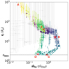 |
Fig. 4. Positions of all observation in the ṁin−rJ plane for the four outbursts of GX 339-4 covered by RXTE/PCA. All data points are shown in gray, and the constrained observations (see text) are color-coded as in Fig. 2. The points in pink are radio-constrained observations of the 2008–2009 failed outburst. Points A–E are placed at the average locations (of the four outbursts) for each phase to illustrate their approximate locations. |
A complete cycle starts in the quiescent state, located at the upper left region of the ṁin−rJ plane; at small ṁin and large transition radius rJ, around point A. The start of the outburst corresponds to a simultaneous increase in ṁin and decrease in rJ until point B, where the system initiates its transition to the soft states. In these intermediate states (from B to C), the spectral evolution is mainly due to a steep decrease in rJ, with a much narrower evolution of the disk accretion rate ṁin. Soft states are characterized by the non-existence of a JED; the system sticks to the rJ = risco line, where only an evolution in ṁin is observed. Eventually, GX 339-4 exhibits a decrease in ṁin until point D, where a JED is rebuilt inside-out. Again, these intermediate states mainly correspond to an increase in rJ, while the evolution in ṁin is barely visible. At point E, GX 339-4 returns to the hard state branch and then decays back towards the quiescent state in point A. Interestingly, we see that the maximum ṁin achieved during the hard state can actually be variable. While outbursts #1, #3, and #4 follow the same track (i.e., they have similar ṁin(B)), outburst #2 reaches a ṁin(B) that is approximately two to three times smaller, Ṁin(B) ≃ 1.0 instead of Ṁin(B) ≃ 2.5−3.0. Some degree of freedom must therefore be allowed in the path. Conversely, the lower soft to hard transition (point D) seems to occur at a similar accretion rate ṁ ≈ 0.2−0.3. These two results were expected since the upper transitions are known to achieve variable luminosities while the lower ones occur roughly at the same luminosity (Maccarone 2003; Dunn et al. 2010). However, this is now translated into physical quantities for the first time.
While four different complete outbursts are shown in Fig. 4, it clearly exhibits a unique pattern followed by all outbursts when only the constrained observations are used. Moreover, the failed outburst (2008–2009, pink dots) also follows the same track, strengthening the idea of a common path. A failed outburst would be the result of the system not reaching a ṁin high enough (or a rJ small enough) to trigger the transition to a soft state. The unique track suggests a hidden link between rJ and ṁin (or ṁ), as rightfully argued in Aneesha et al. (2019). Specifically, the variations of one parameter would be the answer to the variations of the other, presumably rJ reacting to changes in ṁ due to the long timescales involved. While it has already been predicted in the literature (see, e.g., Ferreira et al. 2006; Begelman & Armitage 2014; Kylafis & Belloni 2015), this is to our knowledge the first demonstration of such a link using an observational fitting procedure (see, however, Cabanac et al. 2009; Plant et al. 2015, for similar studies). We call this path a fingerprint, and we expect all sources to be born with one, but that each will present differences originating from the source’s properties, such as the spin of the black hole, or the size or inclination of the system.
3. Evolution of the disk structure during an outburst
We now discuss the changes in the thermal structure of the accretion flow during an outburst. Just as in the previous sections, the results presented in this section are model-dependent: the calculations are performed within the JED-SAD paradigm, and thus rely on its assumptions (Papers II and III) and on the chosen fitting procedure (Paper IV).
3.1. Three routes for energy dissipation
The code we developed and used in this study solves for the thermal structure of the hybrid JED-SAD disk configuration. The following local (vertically integrated) equations are solved at each cylindrical radius r
 (2)
(2)
where we define the total accretion power qacc and the power funneled in the jets qjets = b(r)qacc. We assume that the jets take away 30% of the disk accretion power in the JED portion1 and 0% in the SAD portion (i.e., bJED = 0.3 and bSAD = 0). As a result, the power funneled in the jets solely depends on the JED accretion power qjets = 0.3 qacc, JED. Additionally, we assume that electrons and ions share equal parts of the available energy δ = 0.5 (Yuan & Narayan 2014, see their Sect. 2.2). We also define the collisional Coulomb heat exchange qie, the radiative cooling term qcool, and the advected power transported radially by the ions qadv, i and electrons qadv, e. The local advection term (qadv = qadv, i + qadv, e) can either act as a cooling or a heating term, depending on the sign of the radial derivatives of the internal energy and inflow velocity. We refer the interested reader to Sect. 2 in Paper II.
The global energy budget of our hybrid JED-SAD disk configuration can be obtained by summing the ion and electron energy Eqs. (2), and integrating over all radii [risco, rout]. This provides
 (3)
(3)
where Pα = ∫qα2πrdr for each physical term qα in Eq. (2). The released accretion power Pacc is thus shared between the power carried away by the jets Pjets, the power advected onto the black hole Padv, and the bolometric disk luminosity Lbol = Pcool. It is important to remember that any estimate of these powers is model-dependent and can be subject to important caveats: the observed disk luminosity is only a fraction of Lbol, the spectrum barely provides any clues on the advected power, and determining the power carried away by the two jets is a substantial task. All estimates in the following are thus done within the JED-SAD framework (i.e., subject to its assumptions and the methods used). To use dimensionless terms, we express these quantities in terms of efficiencies by dividing the above equation by Pacc: ηα = Pα/Pacc. These efficiencies verify
 (4)
(4)
where ηjets is the global ejection efficiency, ηadv the global advection efficiency, and ηcool the global radiative efficiency. When the whole disk is in SAD mode, ηcool is roughly constant and around unity, regardless of ṁin. This case is usually referred to as the radiatively efficient situation, where the disk luminosity varies linearly with the accretion rate L ∝ ṁ (or ṁin). When the inner JED is present, powerful jets are launched, which generates a strong radial torque on the accretion flow. This torque accelerates accretion, allowing for optically thin and geometrically thick solutions, increasing the disk vertical extension and advection processes with it: ηcool must then necessarily vary with ṁ and can eventually reach only a fraction of unity. It is therefore much harder to estimate Pacc (and thus ṁ) directly from the observed spectrum when a JED is involved, unless the behavior of ηcool is understood (see below).
3.2. Energy dissipation during an outburst
We show in Sect. 2 that 15 years of GX 339-4 activity results in a characteristic path in the ṁin−rJ plane. For each best fit in this plane we can solve for the thermal structure and derive the various contributions of energy dissipation that reproduce the observed spectrum. We illustrate in Fig. 5 the value of the global ejection efficiency ηjets (top), advection efficiency ηadv (middle), and radiative efficiency ηcool (bottom). For clarity, only the constrained states have been used: hard states with concurrent radio detection, all intermediate states, and all soft states. Equation (4) is satisfied by construction at each observational point, and each symbol color varies from light to dark when ηi varies from 0 to 100%. This means that each symbol is darker in the figure of its dominating process (see color bar). We recall that all the results derived in this section are done within the JED-SAD framework (i.e., they are model-dependent).
As expected, the total power carried away by the jets (ηjets) is always near 30% when rJ ≫ risco because we assumed b = 0.3 in the JED. A significant decrease is finally visible when rJ reaches rJ ≃ 2 risco = 4 (dashed blue line). This is due to the transition to the soft state where very little (but not always zero) energy is channeled in the jets (i.e., ηjets is at most a few percent). As a result, advection and radiation share only 70% of the released power when rJ ≫ risco, and 100% when rJ = risco. Compared to the ejection efficiency, the advection (ηadv) and radiative (ηcool) efficiencies span a much wider range of values: ηadv varies between 0% and 55% and ηcool varies between 15% and 100%. In these two panels, the dashed green line is defined as the locus where ηadv = ηcool = 35%, namely some sort of equipartition between all energetic processes since ηjets = 30%. It is important to note that even when advection has the dominant role in the disk structure, it is never greater than 55%. These results are thus in strong contrast with the advection-dominated accretion flow (ADAF, Narayan & Yi 1995), presumably because of the difference in the shared energy between the ions and the electrons (δ = 0.5 here, δ = 1/2000 for an ADAF).
On the top left side of the dashed green line, advection is larger than radiation (Padv > Pcool), whereas on the bottom right side radiative losses overcome the advected energy (Padv < Pcool). Surprisingly, while all intermediate and soft states are on the same side of the line (Padv < Pcool), there are hard states on both sides of the line (i.e., with Padv < Pcool and with Padv > Pcool). To understand the reasons and implications of this difference we select two hard state solutions (see the two circles in Fig. 5), and discuss them in Sect. 3.3.
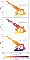 |
Fig. 5. Positions in the ṁin−rJ plane of all the selected constrained states (see Sect. 2.4), indicating each global efficiency: jets ηjets = Pjets/Pacc (top), advection ηadv = Padv/Pacc (middle), and radiation ηcool = Pcool/Pacc (bottom). The green line shows states with equipartition (i.e., ηadv ≈ ηcool ≈ ηjets ≈ 0.30−0.35), while the blue line separates states where ηjets is significant (over the line) or not (under the line). We discuss the two solutions circled in black in more detail in Sect. 3.3 and Fig. 6. |
3.3. Thick and slim disk regimes
We show in Fig. 6 the thermal structure of the two solutions indicated by black circles in Fig. 5. We illustrate the radial evolution of their vertical extension on the y-axis of the top and middle panels. The vertical extension of a given accretion flow is usually expected to increase with ṁin. This is verified here in the standard accretion disk region, where in R = 100 Rg we have H ≃ 1 Rg when ṁ = 0.5 (left) and H ≃ 2 Rg when ṁ = 1.3 (right). In the jet-emitting disk region, however, the disk is much thinner for the highest ṁin because less energy is lost through advection or, alternatively, radiative cooling is more efficient. The vertical extension is thus one of the most striking differences between the two regimes: geometrically thick disks H/R ≳ 0.2 when Padv > Pcool (left) and geometrically slim disks H/R ≲ 0.1 when Pcool > Padv (right). In comparison, as we have seen, a typical standard accretion disk is much thinner with H/R ≈ 0.01−0.02 ≪ 1. We thus label these JED solutions as the “thick” regime when Padv > Pcool and the “slim” regime when Padv < Pcool. It is important to note that even if we only show two specific solutions here, the properties we discuss apply to all thick and slim states, respectively above and below the dashed green line in Fig. 5.
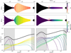 |
Fig. 6. Geometrical shape and spectral energy distribution of the two solutions. Left: JED-SAD solution with rJ = 65 and ṁ = 0.5. Right: JED-SAD solution with rJ = 30 and ṁ = 1.3. For both solutions, the radial distribution of the JED is divided into ten portions. Top and middle panels: radial evolution of the vertical extension of the disk (x-axis at the top) compared to the black hole horizon represented by the black ellipsoid on the right side of each panel. The vertical Thomson optical depth (top) and the electron temperature (middle) are color-coded (top and bottom color bar, respectively). Bottom panels: total emitted spectrum in black with the contribution from the entire SAD (dotted line) and each JED portion (dashed lines), color-coded according to temperature (same as middle panels). The RXTE X-ray range is inside the gray background. |
In addition to their geometrical differences, there are major differences in the thermal structures of the disks (top and middle panels of Fig. 6) and the resulting spectral shape (bottom panel). In the thick regime (left), the JED is optically thin with τT ≲ 0.8 < 1 (in beige–salmon), and the electron temperature is constant over most2 of the different jet-emitting disk annuli: kBTe(rJ)≳100−300 keV (in light green–yellow). As a result, all sub-spectra have a power-law shape with a high energetic cutoff that is barely detectable in the RXTE/PCA spectral band used in this work (bottom panel of Fig. 6). In this case the total SED, computed by summing all annuli, shares the same properties with a power-law shape whose spectral index arises from the combination of all the sub-power laws. In the slim disk regime (right), the disk is optically slim with τT ≳ 3 > 1 (purple), and the electron temperature varies radially between ≤10 and 200 keV in the JED (dark blue to green). Due to these radial variations of optical depth and temperature, the sub-spectra of the JEDs now have more pronounced spectral differences. For instance, the high-energy cutoff of each sub-spectra appears below 200 keV. The sum of all these sub-spectra still gives a power-law shape, but now with a detectable cutoff around 100 keV for high-luminosity hard states, consistently with Motta et al. (2009).
There is thus an important transition for the JED within all the hard states observed: from the thick disk regime to the slim disk regime. Thick states are observed at low-luminosity and their energy budgets are ηadv ≳ 50%, ηcool ≲ 20%, and ηjets = 30%. Slim states are observed at high-luminosity and their energy budgets are ηadv ≃ 30%, ηcool ≃ 40%, and ηjets = 30%. This difference is minor in theory since both these regimes are near equipartition with only a slight imbalance between advection and radiation. Moreover, the slopes of both total spectra are quite similar with ΓPL ≈ 1.5−2, showing no clear differences between the two regimes (but see Sect. 4.2). However, we show in the following section that the transition between these two regimes has a major observational impact because the radiative efficiency varies from ≲20% to 40% (i.e., more than a factor of two). Additionally, the spectral shapes at each radius involved are disparate between thick and slim regimes, suggesting that distinct processes could be producing the spectra at different luminosities. This discrepancy could be visible in the evolution of the reflection spectra, in the time-lags observed, and even in the quasi-periodic oscillations. These questions are far beyond the scope of the present paper, although we will see later on that the transition from thick disk to slim disk is directly visible in the variation of the power-law spectral index Γ (see Figs. 7 and 8).
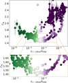 |
Fig. 7. Evolution of the power-law index ΓPL of each spectrum (Clavel et al. 2016) as a function of its luminosity in the 1−10 keV range. All four outbursts during the 2000s are overplotted (color-coding as in Fig. 9). Bottom panel: zoom-in on the zone inside the orange dashed rectangle in the top panel. For clarity, we do not show observations when ΓPL is unconstrained (soft states), but the usual values lie in the ΓPL ≈ 2.0−3.0 range. |
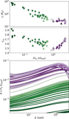 |
Fig. 8. Subset of all hard state observations with detected radio fluxes, using the same color-coding as in Fig. 9. The symbol shapes show the rising (up-pointing triangle) and decaying (down-pointing triangle) hard state. Top: distribution of these observations in the ṁin−rJ plane (x-axis at top). Middle: spectral index of the power law ΓPL from the Clavel et al. (2016) as function of the ṁin from our fits. Bottom: theoretical spectra associated with each solution (rJṁin) in the (theoretical) RXTE range 2−300 keV. |
4. Radiative efficiency and the radio–X-ray correlation
4.1. Radiative efficiency of the accretion flow
We now focus on the disk radiative efficiency. For each observation, we show in Fig. 9 the evolution of rJ (top), the bolometric radiative efficiency (middle), and the unabsorbed X-ray radiative efficiency (1−10 keV, bottom) as function of the disk inner accretion rate ṁin. Both radiative efficiencies are defined as the ratio of their associated luminosity with respect to the total available power Ṁinc2, labeled εbol = Lbol/(Ṁinc2) and ε1−10 = L1−10 keV/(Ṁinc2) in all the following. The bolometric radiative efficiency can be linked to the cooling efficiency with εbol = ηcoolηacc, where ηacc = 1/(2risco)=1/4 is the accretion efficiency of a black hole of spin 0.93. In other words, an accretion flow radiating 100 % of its accretion power will only emit 25 % of its total available power (i.e., 25 %Ṁinc2), while a flow radiating 10 % of its accretion power will emit 2.5 % Ṁinc2. We note that the top panel of Fig. 9 is the same as the bottom panel of Fig. 5, but with an inverted y-axis and using different color maps and scales: the color now indicates the ratio of advected to radiated powers. This allows us to highlight the two different JED regimes discussed in Sect. 3.2: thick in green, slim in purple, as well as their transition in white. The color bar includes the state with minimum radiative power (Pcool ≈ 0.3 Padv), whereas the maximum of the color bar is set to Pcool = 1.7 Padv, even if it reaches Pcool ≈ 104 Padv in the soft states where only a SAD is present. We again recall that the results derived in this section are done within the JED-SAD framework (i.e., they are model-dependent).
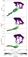 |
Fig. 9. Observations of GX 339-4 in the ṁin−rJ plane (top), bolometric luminosity (Lbol) computed from our model (middle), and 1−10 keV luminosity (L1−10 keV) as function of ṁin (bottom). In all panels the color is the ratio of bolometric radiated power to the power advected (see color bar). The different lines are shown in orange to illustrate different regimes: solid when |

These different portions of the outburst are directly visible in the evolution of the bolometric radiative efficiency εbol = Lbol/(Ṁinc2) as a function of ṁin (middle panel). This figure is a slight modification of the ṁin−rJ plane because the thermal structure at a given ṁin strongly depends on rJ. However, variations in ṁin produce a more complicated picture, especially at the transition between the two states (white). At low ṁin, we are in the thick disk regime (green) with Lbol ≲ 0.06 Ṁinc2 (i.e., εbol ≲ 6%; dashed orange line). As ṁin increases, we transition to the slim disk regime (violet and purple) where Lbol > 0.12 Ṁinc2 (i.e., εbol > 12%; dotted orange line). Interestingly, the transition from thick to slim (in white) follows an εbol ∝ ṁin track showed in solid orange. A regime with εbol ∝ ṁin (i.e.,  ) has been labeled as radiatively inefficient in the past (see, e.g., Coriat et al. 2011, Sect. 4.3.3). In our case, however, there is no such regime. The portion with
  is only a transition between two different states of different radiative efficiencies, both of which are actually radiatively efficient (as opposed to the flows that are usually considered radiatively inefficient, see below). As rJ decreases to risco, the radiative efficiency increases because the jet-emitting disk radial extension shrinks to give more ground to the standard accretion disk. We finally reach a maximum value of Lbol ≈ 0.25 Ṁinc2 (i.e., εbol ≈ 25% when only a standard accretion disk is present.
In the bottom panel of Fig. 9, the evolution with the accretion rate is altered by the energy band chosen (see Paper III, Sect. 4.2). The thick disk regime (in green), where bolometric luminosity increased moderately with ṁin, now follows a nearly constant efficiency when only looking at the 1−10 keV range. This gives rise to a first phase with constant ε1−10 (i.e., L1−10 keV ∝ ṁin; orange dashed line). However, the phase Lbol ∝ ṁin observed during the slim disk regime (violet) has disappeared. Instead, the transition from thick to slim seems to merge with the slim disk regime itself. This gives birth to a second phase with a surprisingly steep slope ε1−10 ∝ ṁin (i.e.,  ; orange solid line). One usually associates this phase to a radiatively inefficient accretion flow, but around 40% of the accretion power is still radiated away in our model. Both phases (dashed and solid lines) should instead be considered as radiatively efficient, with around εbol ≈ 6% to 12% of the total available power3 radiated away, and ε1−10 ≈ 0.5% to 3% in the 1−10 keV band. However, we can compare these regimes to an even more efficient regime during the soft-state rJ = risco (dark violet), where all the accretion power is radiated away (i.e., εbol ≈ 25%) with ε1−10 ≈ 10−15% in the soft X-ray band.
These results illustrate that the presence of two regimes and the difference in their radiative efficiency values generates different slopes in the L−Ṁ evolution. One should thus be very careful when discussing radiative efficiencies. Accretion rate changes lead to structural changes that can lead to misconceptions or even misinterpretations when filtered through a given energy range. While we do observe a  phase during the outburst, this phase is never associated with what is usually called a radiatively inefficient accretion flow since the flow always radiates more than 20% of its available accretion power (about 5% of the total available power).
4.2. Evolution of the power-law index
In the previous sections of this paper we illustrate the change in the thermal structure of the accretion flow during the hard state. More precisely, we show that there are two different regimes depending on the thermal structure of the disk: thick disk when Padv > Pcool and slim disk when Padv < Pcool. However, all the changes presented are model dependent: all calculations are performed within the JED-SAD paradigm, and thus rely on its assumptions (Papers II and III) and on the chosen fitting procedure (Papers IV). Such a transition has already been observed using model-independent estimates: the hardness ratio or the spectral index of the power law (see, e.g., Sobolewska et al. 2011). In this work we decided to use the spectral index because any hardness ratio requires a choice of two spectral bands and we wanted to remain as generic as possible.
We show in Fig. 7 the evolution of the spectral index of the power law from Clavel et al. (2016). We show all observations during the four outbursts except when ΓPL is unconstrained in the soft state. The top panel shows the entire range of values, while the bottom panel shows a zoom-in on the transition between thick and slim regimes (see below). In this figure an outburst starts on the left side with ΓPL ≈ 1.8−2.0 and L1−10 keV ≈ 10−4 LEdd, and then runs through the cycle counterclockwise. All hard states are roughly found when ΓPL ≤ 1.8−2.0, while soft states are around ΓPL ≈ 2.2−2.6. The same color map as in Fig. 9 is used here, illustrating the transition from thick disk solutions (Pcool < Padv, in green) to slim disk solutions (Pcool > Padv, in purple). As already seen in Fig. 9 (bottom panel), the transition (in white) from the thick to the slim solution happens around L1−10 keV ≈ 5 × 10⁻³ − 10−2 LEdd. What is interesting here is that the transition is also concurrent with a change in the evolution of ΓPL (see zoomed-in portion in bottom panel). When L1−10 keV ≤ 5 × 10⁻³ LEdd, ΓPL decreases with luminosity, but when L1−10 keV ≥ 10−2 LEdd, ΓPL increases with luminosity.
There is thus an important change in the spectral shape around4L1−10 keV ≃ 5 × 10⁻³ LEdd. The evolution of ΓPL is fully consistent with the locus of the thick to slim transition expected from our JED-SAD framework. The evolution in ΓPL in the hard state appears then as a convenient tool to trace the change in the accretion flow structure.
4.3. Evolution of the spectral shape during the hard state
In this section we consider only the constrained hard states (i.e., the hard states when radio flux has been observed). These states are all fit with rJ ≫ risco (i.e., with 30% of the power channeled in the jets and 70% shared between Padv and Pcool). We show in Fig. 8 the ṁin−rJ plane (top), the power-law spectral index ΓPL (middle), and the associated best fit JED-SAD spectra in the 2−300 keV range (bottom) for each observation. The color scale is as in Fig. 9: thick disk spectra in green (Pcool < Padv), slim disk spectra in purple (Pcool > Padv), and the transition (equipartition Pcool = Padv) in white.
We see in the ṁin−rJ plane (top panel) that the transition between the thick and the slim regimes is barely visible; without the colors we could not locate the transition on this panel, around rJ ≃ 30 and ṁin ≃ 0.75. As seen in Sect. 4.1, the luminosity evolves as  at the transition between the two regimes. A slight increase in ṁin then translates into a dramatic rise in luminosity: we should expect the transition between these regimes to generate a gap in luminosity. This gap is indeed observed in the hard state spectral evolution5, as seen in the bottom panel of Fig. 8 and already discussed in Koljonen & Russell (2019). In our model the observed gap simply originates from a change in the thermal structure of the accretion flow, and eventually in radiative efficiency.
As discussed in Sect. 4.2, while the change in radiative efficiency during an outburst is model-dependent, the spectral index of the power law ΓPL is not. We show in the middle panel of Fig. 8 the evolution of ΓPL as a function of ṁin for all our constrained hard states6. We see in this figure that the gap in luminosity (in white) coincides with a change in the evolution of ΓPL. At low accretion rates (or luminosity, see Fig. 7), the power-law spectral index decreases as ṁin increases. At high accretion rates, however, the spectral index now clearly increases with ṁin. There are thus two different groups of hard state spectra, corresponding to the two different regimes discussed in Sect. 3.2: thick disk and slim disk. The spectral shapes are very similar between the two regimes and mainly differ by their fluxes. As a result, finding this transition can be tricky. We illustrate in this work that one can do so either by using our JED-SAD model, or simply by tracking the changes in ΓPL (see, e.g., Sobolewska et al. 2011). Because we believe the physical structure of the accretion flow to be similar in all X-ray binaries, we expect this transition to be present for all objects around a similar luminosity (i.e., around L1−10 keV ≈ 10−3 − 10−2 LEdd). Moreover, we expect this transition to have an impact on the radio–X-ray correlation, as discussed in Sect. 4.4.
4.4. The radio–X-ray correlation
In this section we only isolate the constrained hard states as in Sect. 4.3, and we focus on the impact of the radiative efficiency regimes on the radio–X-ray correlation  . In this correlation, the luminosity LR is derived from the observed radio flux densities, usually around 5−9 GHz, and LX from the flux observed in either the 1−10 keV or the 3−9 keV energy range (see, e.g., Coriat et al. 2011; Corbel et al. 2013). We use the 8.6−9.0 GHz radio band and the 1−10 keV X-ray range to be consistent with the known correlation from Corbel et al. (2013). We show in Fig. 10 the observed radio luminosity LR as a function of the observed 1−10 keV (top) and bolometric (bottom) X-ray luminosities. We use the same color-code as in Fig. 9 (i.e., thick hard states in green, slim hard states in purple, transition in white). We recall that the top panel of Fig. 10 is purely observed data, while the bottom panel shows bolometric fluxes that have been obtained using our model. As a result, the top panel is model-independent, but the bottom panel is not and it relies on our assumptions and fitting procedure.
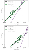 |
Fig. 10. Correlations between the observed radio fluxes and the fitted X-ray flux emitted by the accretion flow in two different energy ranges: classical 1−10 keV range (top) and bolometric (bottom). In each panel the symbol shows a rising (up-pointing triangle) or decaying (down-pointing triangle) hard state, and the color is the ratio Pcool/Padv of the radiative to the advected power (see color bar in Fig. 8). The solid lines indicate our fits: global correlations (black), with only Padv > Pcool solutions (green) and with only Padv < Pcool solutions (purple). A dashed line illustrates the location of the crossing point of the thick disk and slim disk correlations. |
When we fit all the observations together in the 1−10 keV range (black line) we retrieve the usual correlation with a = 0.57 ± 0.03 ≃ 0.6 (Corbel et al. 2003, 2013; Gallo et al. 2003; Coriat et al. 2011). This was expected since we use the same X-ray ranges as Corbel et al. (2013). However, things become interesting when the two different regimes are considered independently. While we obtain a similar fit using only the thick disk observations (a = 0.57 ± 0.06), the correlation becomes much steeper in the case of slim disk observations (a = 1.02 ± 0.16). We believe that the reason for this discrepancy is the sensitivity of the disk radiative efficiency ε1−10 to changes in ṁin, as explained in Sect. 4.1. When the system transitions from the thick to the slim regimes both rJ and ṁin undergo steady changes. While the X-ray emission shows swift changes in radiative efficiency near the equipartition Pcool = Padv zone (white), the jet radio emission undergoes slow and steady changes: there is no apparent reason for its radiative efficiency to vary as well. This produces the observed plateau in the LR − LX curve around LR = 7 × 10⁻⁹ LEdd, providing a natural explanation for the wiggles seen in the radio–X-ray correlation curve for GX 339-4. We note, however, that the locus of the wiggles corresponds to the soft to hard transition (i.e., the rebuilding of the jets). It is thus possible that these wiggles are a result of the jet building, as is discussed in Barnier et al. (2022).
For completeness, we show in the bottom panel of Fig. 10 the radio luminosity as a function of the bolometric luminosity. We recall here that the bolometric luminosity is a result of our physical model, not an extrapolation of the disk and power-law shapes. When including all observations with detected radio and X-rays, we find a similar correlation with a = 0.63 ± 0.03. However, there is now an even clearer difference between the green and the purple states, the former providing a correlation with a = 0.49 ± 0.04 and the latter a much steeper exponent a = 1.55 ± 0.17. This result shows that these wiggles are not an effect of the spectral energy range used for observations and should always be seen. However, the critical luminosity Lc where the two correlations meet, namely where a break with the low-luminosity branch becomes distinguishable, does depend on the energy band. For GX 339-4 and the set of dynamical parameters used, the critical luminosity in the 1−10 keV energy range is Lc ≃ 3 × 10⁻² LEdd ≃ 2 × 1037 erg s−1 and becomes Lc ≃ 12 × 10−2 LEdd ≃ 9 × 1037 erg s−1 in bolometric. As said above, these luminosities happen to be close to where the actual hysteresis cycle starts, namely the point in the HID where the rising hard state branch meets the decaying horizontal soft-to-hard branch. As a result, all hard states with LX > Lc were observed during the rising phase (up-pointing triangles in Figs. 8 and 10) whereas most (but not all) of the hard states with LX < Lc were observed during the decaying state (down-pointing triangles). This raises questions about the possible differences between rising and decaying phases (Islam & Zdziarski 2018; Barnier et al. 2022). However, our modeling shows that this may only be due to the evolution of the JED radiative efficiency as the disk accretion rate increases.
4.5. The existence of outliers
An important aspect of the radio–X-ray correlation is the presence of outliers; namely X-ray sources that do not follow the standard correlation, but a rather steeper correlation (at least at sufficiently high flux) with LR ∝ L≈1.4 (Coriat et al. 2011; Gallo et al. 2012; Corbel et al. 2013). In the present study we show that we retrieve the standard correlation followed by GX 339-4 when all hard states are used. However, we find LR ∝ L≈1−1.5 when considering only the slim hard states. This result suggests that GX 339-4 would behave similarly to H 1743-322, where two different tracks LR ∝ L≤0.6 and LR ∝ L≥1.0 are observed (Corbel et al. 2013, Fig. 9). Interestingly, most outliers seem to be observed at high luminosities (L1−10 keV ≥ 1036 erg s−1) (i.e., where the inner jet-emitting disk becomes slim). This raises the question of the existence of outliers: Do outliers exist, or is the observed sample only located in this slim disk regime?
To answer these questions, similar studies on more outbursts from both GX 339-4 and from other sources would need to be performed. Such a study should also investigate the uniqueness of the transition luminosity. This transition in the disk radiative efficiency, seen as a plateau in the LR − LX correlation, is inherent to our JED-SAD model (at least for the parameters used for GX 339-4). If such a transition is not observed in other objects then the change in the slope observed in outliers cannot arise from changes in the disk radiative efficiency. This would mean that another physical factor must be at work, most probably related to the jet emission itself: collimation properties, internal shock conditions (Malzac 2013, 2014; Marino et al. 2020), or even the interplay between the Blandford & Payne jet emitted from the JED and the inner spine emitted from the black hole ergosphere (Blandford & Znajek 1977). This opens quite interesting prospects, far beyond the scope of the present study.
5. Caveats
Our JED-SAD modelling comes with some caveats. These caveats were thoroughly discussed in the previous papers in this series, but we recall here the most important points.
We perform our calculations using a Newtonian potential and a non-relativistic version of the radiative transfer code BELM (Belmont et al. 2008; Belmont 2009). As the disk material plunges into the black hole, a smaller fraction of the mechanical energy is actually released: the Novikov & Thorne (1973) turbulent dissipation is smaller than in the Shakura & Sunyaev (1973) non-relativistic disk (see Page & Thorne 1974 and also discussion in Penna et al. 2012). We thus expect our model to underestimate the disk accretion rate ṁin for radii rJ ≤ 6. This approximation is not crucial for large transition radii rJ ≫ risco (i.e., for the states thoroughly studied in this paper), but it can become important when discussing the shape of the track followed in the ṁin−rJ plane at small rJ. This will be discussed in a forthcoming work.
The calculations performed in this paper only use the 3−25 keV RXTE/PCA data, in which the high-energy cutoffs cannot be constrained. Because they are unreliable in this range, the cutoffs seen in Fig. 8 have not been implemented in the fitting procedure. However, their presence is inevitable within the JED-SAD paradigm. These cutoffs were not necessary in the fits, but they are unavoidable in the resulting spectra. This can be tested in broadband (> 10 keV) data sets, as is done in the case of Swift+NICER+NuSTAR observations from the black hole X-ray binary MAXI J1820+070 (Marino et al. 2021). This may also explain the possible differences with the real observed cutoff that can be seen in Fig. 2 of Koljonen & Russell (2019).
In this work we use the equation that was solved in Marcel et al. (2018b) to separate all energy components: Pacc = Pjets + Padv + Pcool. However, it has recently been argued that winds could be present at all times during an outburst (see, e.g., Miller et al. 2015, and also Petrucci et al. 2021). A more complete equation should thus be Pacc = Pjets + Padv + Pcool + Pwinds at each radius, and with Pjets = 0 or Pwinds = 0 depending on whether jets and/or winds are produced. In our view, winds would be produced in the SAD portion, hence not affecting the JED. We have thus decided to neglect the power carried away by the winds at all times (i.e., Pwinds = 0). On a similar note, all observed soft states display non-thermal tails generally observed above a few keV: the hard tail (McConnell et al. 2002; Remillard & McClintock 2006). Within our framework, this hard component is thought to be related to coronal dissipation and the production of a non-thermal electron population (see, e.g., Galeev et al. 1979; Gierliński et al. 1999). This non-thermal population is not taken into account, however, and our treatment of the hard tail is parametric (see discussion and Fig. 5 in Paper III). This may also lead to some uncertainties on the energy equation during the soft states (i.e., not relevant in the radiative efficiency and radio–X-ray correlation we discussed). Moreover, non-thermal effects could also have an impact on the disk structure and its equilibrium during any given state (McConnell et al. 2002; Malzac & Belmont 2009), but we chose to ignore these effects in this work.
We showed in Sect. 4.4 that the wiggles seen in the radio–X-ray correlation of GX 339-4 can be explained by simple changes in the disk structure. Within our model, these wiggles are a simple consequence of variations of the disk radiative efficiency with the disk accretion rate. However, in our study, the radio emission along the cycles is computed using three simplifying assumptions. First, we use b = 0.3 throughout the entire study (i.e., assuming that 30% of the JED power is funneled in the jets). While it would be more physical to assume b to be a function of the physical structure of the accretion flow, this choice is justified both physically (Petrucci et al. 2010) and spectrally (Marcel et al. 2018b). Second, a phenomenological expression for the radio flux FR(ṁin,rJ), see Eq. (3) and discussion in Paper IV. Third, we used a unique normalization factor f̃R = 4.5 × 10⁻¹⁰ for all cycles, allowing us to qualitatively reproduce the radio–X-ray correlation (see Paper V). There is, however, no physical reason for such a value to be unique. A deeper examination of the radio emission light curves (Figs. 2 and 3 in Paper V) reveals that a better tuning could be done in order to properly describe the radio. In particular, there might be a possible difference between the rising states and the decaying states, or even changes within a given outburst phase. Assuming a function FR with a unique and constant f̃R might have generated biases in our results, especially at very low flux when the X-ray spectral shape is not enough to constrain rJ. This is an important question, especially since recent studies found possible differences in both the iron line profiles (Wang-Ji et al. 2018; Wang et al. 2020, and references therein) and the radio–X-ray correlation (Islam & Zdziarski 2018, but see Sect. 4.4). We will address this issue in greater detail in a forthcoming paper (Barnier et al. 2022).
6. Discussion and conclusion
We use the results from our previous work (Ferreira et al. 2006; Marcel et al. 2018b,a, 2019) and compare the temporal evolution of the two dynamical parameters rJ(t) and ṁin(t). We show that, within the JED-SAD paradigm, their temporal evolution vary significantly between outbursts (see Sect. 2.2). However, when illustrated in a rJ(ṁ) diagram, the path followed shows clear similarities for all considered outbursts of GX 339-4 : a fingerprint. While expected, this is an important result and the physical interpretation of this fingerprint will be proposed in a following paper. Moreover, we can estimate the different processes of energy dissipation in the accretion flow: radiation (Pcool), advection (Padv), and ejection (Pjets). We thus use the model to estimate each of these powers for all the observations in the fingerprint. We show that three major outcomes can be drawn from this study.
First, the concept of radiative efficiency can be misleading. In particular, we show that within our framework there are two major slopes in the correlation between the X-ray luminosity and the accretion rate: LX ∝ ṁin at low-luminosity and  at high luminosity. In our model, we explain these different slopes by the changes observed in radiative efficiency. These two portions have been observed in the past and labeled as radiatively efficient and radiatively inefficient (see, e.g., Coriat et al. 2011). Within our framework we show that, for ṁin > 10−2, the disk is in fact never radiatively inefficient because the accretion flow always radiate more than 15−20% of its accretion power. We also argue that the energy band chosen can have a key impact on the slopes obtained between LX and ṁin, often making any estimate unreliable.
Second, we show that there are two different types of hard state spectra, associated with the thermal state of the accretion flow. At low luminosity, the accretion flow is optically thin and geometrically thick, and the total spectrum is that of a simple power law with undetected cutoff: the thick disk regime. At high luminosity, the thermal structure is optically and geometrically slim, and the total spectrum is very similar to the previous power law, although this time with a visible cutoff around 50−100 keV: the slim disk regime. In the JED-SAD paradigm this transition unavoidably happens during the rise in the hard state due to the structure of the accretion flow. We thus predict that a similar transition should be observed in other objects or outbursts. We also show that this transition between thick and slim disk regimes is consistent with a change in the evolution of the power-law index ΓPL, as already observed in Sobolewska et al. (2011).
Third, the evolution of the radiative efficiency during the hard state has an important impact on the radio–X-ray correlation. While the radio is thought to be linked to the jets structure, in our modelling the X-rays originate from the accretion flow. In consequence, changes in the accretion flow radiative efficiency have a direct impact on the X-rays, but not7 on the radio. In the radio–X-ray correlation, the changes in X-ray radiative efficiency translate into two different slopes separated by a sort of plateau, see Fig. 10. When all hard states are considered, we retrieve the radio–X-ray correlation  (Corbel et al. 2013). When only the most luminous hard states are considered, however, the correlation follows a much steeper slope
  , up to
  depending on the energy ranges considered. Such steep slopes have been associated with a second group of X-ray binaries, labeled outliers, thought of as having a different behavior (see, e.g., Huang et al. 2014). We provide here a possible alternate explanation: these outliers could simply be observed at higher accretion rates where the disk radiative efficiency evolves in the slim disk state, rather than the usual thick disk state. Extending this work to other sources, and especially to outliers, should provide valuable constraints and allow this issue to be firmly addressed.
Typical values lie in the range 0−80 % (i.e., b = 0−0.8), but we chose b = 0.3 consistently with the other parameters of the JED (Ferreira 1997, and references therein).
The first two portions in the JED (R/Rg ∈ [65, 50] and R/Rg ∈ [50, 35]) are much colder, with respective temperatures of kBTe ≤ 10 keV and kBTe ≃ 100 keV, because the cold and geometrically thin SAD in r > rJ cools down the JED through radiation and advection processes (see Sect. 2 in Paper III).
Not to be confused with the accretion power Pacc, different by a factor ηacc = 1/(2risco)=0.25 here.
The mass of GX 339-4 is not well constrained, and this luminosity could actually lie anywhere in the range L1−10 keV ≈ 10−3 − 10−2 LEdd.
The absence of observations at that luminosity could also be a result of the observational strategy. For example, outburst #4 was first detected at a luminosity higher than this gap.
We show ΓPL as a function of ṁin to better compare with the rJ(ṁin) curve, but a similar shape is naturally recovered when represented as a function of the X-ray luminosity (see bottom panel of Fig. 7).
This is true under the assumption that the local disk structure (e.g., vertical extension) has no impact on the production of jets. While this is false in general (Ferreira 1997), it was a working assumption in this series of papers and we remain consistent here.
Acknowledgments
We would like to thank the referee for their useful and thoughtful comments that helped improve the manuscript. We are thankful to the European Research Council (ERC) for support under the European Union’s Horizon 2020 research and innovation programme (grant 834203; G.M. and C.S.R.), as well as the UK Science and Technology Facilities Council (STFC) for support under Consolidated Grant ST/S000623/1 (C.S.R.). This work was initiated under funding support from the french research national agency (CHAOS project ANR-12-BS05-0009, https://ipag.osug.fr/ANR-CHAOS//project.html), the centre national d’études spatiales (CNES), and the programme national des hautes énergies (PNHE). A.M. acknowledges a financial contribution from the agreement ASI-INAF n.2017-14-H.0, from the INAF mainstream grant (PI: T. Belloni, A. De Rosa) and from the HERMES project financed by the Italian Space Agency (ASI) Agreement n. 2016/13 U.O.. This research has made use of data, software, and/or web tools obtained from the high energy astrophysics science archive research center (HEASARC), a service of the astrophysics science division at NASA/GSFC. All the figures in this paper were produced using the MATPLOTLIB package (Hunter 2007).
References
- Aneesha, U., Mandal, S., & Sreehari, H. 2019, MNRAS, 486, 2705 [NASA ADS] [CrossRef] [Google Scholar]
- Balbus, S. A. 2003, ARA&A, 41, 555 [Google Scholar]
- Balbus, S. A., & Hawley, J. F. 1991, ApJ, 376, 214 [Google Scholar]
- Barnier, S., Petrucci, P. O., Ferreira, J., et al. 2022, A&A, 657, A11 [NASA ADS] [CrossRef] [EDP Sciences] [Google Scholar]
- Begelman, M. C., & Armitage, P. J. 2014, ApJ, 782, L18 [NASA ADS] [CrossRef] [Google Scholar]
- Belmont, R. 2009, A&A, 506, 589 [NASA ADS] [CrossRef] [EDP Sciences] [Google Scholar]
- Belmont, R., Malzac, J., & Marcowith, A. 2008, A&A, 491, 617 [NASA ADS] [CrossRef] [EDP Sciences] [Google Scholar]
- Blandford, R. D., & Begelman, M. C. 1999, MNRAS, 303, L1 [NASA ADS] [CrossRef] [Google Scholar]
- Blandford, R. D., & Payne, D. G. 1982, MNRAS, 199, 883 [CrossRef] [Google Scholar]
- Blandford, R. D., & Znajek, R. L. 1977, MNRAS, 179, 433 [NASA ADS] [CrossRef] [Google Scholar]
- Cabanac, C., Fender, R. P., Dunn, R. J. H., & Körding, E. G. 2009, MNRAS, 396, 1415 [NASA ADS] [CrossRef] [Google Scholar]
- Clavel, M., Rodriguez, J., Corbel, S., & Coriat, M. 2016, Astron. Nachr., 337, 435 [Google Scholar]
- Corbel, S., Nowak, M. A., Fender, R. P., Tzioumis, A. K., & Markoff, S. 2003, A&A, 400, 1007 [NASA ADS] [CrossRef] [EDP Sciences] [Google Scholar]
- Corbel, S., Coriat, M., Brocksopp, C., et al. 2013, MNRAS, 428, 2500 [Google Scholar]
- Coriat, M., Corbel, S., Prat, L., et al. 2011, MNRAS, 414, 677 [Google Scholar]
- Done, C., Gierliński, M., & Kubota, A. 2007, A&ARv, 15, 1 [Google Scholar]
- Dunn, R. J. H., Fender, R. P., Körding, E. G., Belloni, T., & Cabanac, C. 2010, MNRAS, 403, 61 [Google Scholar]
- Eddington, A. S. 1926, The Internal Constitution of the Stars [Google Scholar]
- Esin, A. A., McClintock, J. E., & Narayan, R. 1997, ApJ, 489, 865 [NASA ADS] [CrossRef] [Google Scholar]
- Espinasse, M., & Fender, R. 2018, MNRAS, 473, 4122 [Google Scholar]
- Ferreira, J. 1997, A&A, 319, 340 [Google Scholar]
- Ferreira, J., & Pelletier, G. 1993a, A&A, 276, 625 [NASA ADS] [Google Scholar]
- Ferreira, J., & Pelletier, G. 1993b, A&A, 276, 637 [NASA ADS] [Google Scholar]
- Ferreira, J., & Pelletier, G. 1995, A&A, 295, 807 [NASA ADS] [Google Scholar]
- Ferreira, J., Petrucci, P. O., Henri, G., Saugé, L., & Pelletier, G. 2006, A&A, 447, 813 [NASA ADS] [CrossRef] [EDP Sciences] [Google Scholar]
- Galeev, A. A., Rosner, R., & Vaiana, G. S. 1979, ApJ, 229, 318 [NASA ADS] [CrossRef] [Google Scholar]
- Gallo, E., Fender, R. P., & Pooley, G. G. 2003, MNRAS, 344, 60 [Google Scholar]
- Gallo, E., Miller, B. P., & Fender, R. 2012, MNRAS, 423, 590 [Google Scholar]
- Gallo, E., Degenaar, N., & van den Eijnden, J. 2018, MNRAS, 478, L132 [Google Scholar]
- Gierliński, M., Zdziarski, A. A., Poutanen, J., et al. 1999, MNRAS, 309, 496 [CrossRef] [Google Scholar]
- Hannikainen, D., Hunstead, R., & Campbell-Wilson, D. 1998, New Astron. Rev., 42, 601 [Google Scholar]
- Heida, M., Jonker, P. G., Torres, M. A. P., & Chiavassa, A. 2017, ApJ, 846, 132 [Google Scholar]
- Huang, C.-Y., Wu, Q., & Wang, D.-X. 2014, MNRAS, 440, 965 [NASA ADS] [CrossRef] [Google Scholar]
- Hunter, J. D. 2007, Comput. Sci. Eng., 9, 90 [NASA ADS] [CrossRef] [Google Scholar]
- Islam, N., & Zdziarski, A. A. 2018, MNRAS, 481, 4513 [Google Scholar]
- Jacquemin-Ide, J., Ferreira, J., & Lesur, G. 2019, MNRAS, 490, 3112 [Google Scholar]
- Jacquemin-Ide, J., Lesur, G., & Ferreira, J. 2021, A&A, 647, A192 [EDP Sciences] [Google Scholar]
- Koljonen, K. I. I., & Russell, D. M. 2019, ApJ, 871, 26 [Google Scholar]
- Kylafis, N. D., & Belloni, T. M. 2015, A&A, 574, A133 [NASA ADS] [CrossRef] [EDP Sciences] [Google Scholar]
- Liska, M., Tchekhovskoy, A., Ingram, A., & van der Klis, M. 2019, MNRAS, 487, 550 [CrossRef] [Google Scholar]
- Maccarone, T. J. 2003, A&A, 409, 697 [NASA ADS] [CrossRef] [EDP Sciences] [Google Scholar]
- Malzac, J. 2013, MNRAS, 429, L20 [NASA ADS] [CrossRef] [Google Scholar]
- Malzac, J. 2014, MNRAS, 443, 299 [NASA ADS] [CrossRef] [Google Scholar]
- Malzac, J., & Belmont, R. 2009, MNRAS, 392, 570 [CrossRef] [Google Scholar]
- Marcel, G., Ferreira, J., Petrucci, P. O., et al. 2018a, A&A, 617, A46 [NASA ADS] [CrossRef] [EDP Sciences] [Google Scholar]
- Marcel, G., Ferreira, J., Petrucci, P. O., et al. 2018b, A&A, 615, A57 [NASA ADS] [CrossRef] [EDP Sciences] [Google Scholar]
- Marcel, G., Ferreira, J., Clavel, M., et al. 2019, A&A, 626, A115 [NASA ADS] [CrossRef] [EDP Sciences] [Google Scholar]
- Marcel, G., Cangemi, F., Rodriguez, J., et al. 2020, A&A, 640, A18 [EDP Sciences] [Google Scholar]
- Marino, A., Malzac, J., Del Santo, M., et al. 2020, MNRAS, 498, 3351 [CrossRef] [Google Scholar]
- Marino, A., Barnier, S., Petrucci, P. O., et al. 2021, A&A, 656, A63 [NASA ADS] [CrossRef] [EDP Sciences] [Google Scholar]
- McConnell, M. L., Zdziarski, A. A., Bennett, K., et al. 2002, ApJ, 572, 984 [NASA ADS] [CrossRef] [Google Scholar]
- Meyer, F., & Meyer-Hofmeister, E. 1994, A&A, 288, 175 [NASA ADS] [Google Scholar]
- Meyer-Hofmeister, E., Liu, B. F., & Meyer, F. 2005, A&A, 432, 181 [NASA ADS] [CrossRef] [EDP Sciences] [Google Scholar]
- Miller, J. M., Fabian, A. C., Reynolds, C. S., et al. 2004, ApJ, 606, L131 [NASA ADS] [CrossRef] [Google Scholar]
- Miller, J. M., Fabian, A. C., Kaastra, J., et al. 2015, ApJ, 814, 87 [NASA ADS] [CrossRef] [Google Scholar]
- Motta, S., Belloni, T., & Homan, J. 2009, MNRAS, 400, 1603 [CrossRef] [Google Scholar]
- Muñoz-Darias, T., Casares, J., & Martínez-Pais, I. G. 2008, MNRAS, 385, 2205 [Google Scholar]
- Narayan, R., & Yi, I. 1995, ApJ, 444, 231 [Google Scholar]
- Novikov, I. D., & Thorne, K. S. 1973, in Black Holes (Les Astres Occlus), 343 [Google Scholar]
- Page, D. N., & Thorne, K. S. 1974, ApJ, 191, 499 [NASA ADS] [CrossRef] [Google Scholar]
- Parker, M. L., Tomsick, J. A., Kennea, J. A., et al. 2016, ApJ, 821, L6 [Google Scholar]
- Penna, R. F., Sąowski, A., & McKinney, J. C. 2012, MNRAS, 420, 684 [NASA ADS] [CrossRef] [Google Scholar]
- Petrucci, P.-O., Ferreira, J., Henri, G., & Pelletier, G. 2008, MNRAS, 385, L88 [NASA ADS] [CrossRef] [Google Scholar]
- Petrucci, P. O., Ferreira, J., Henri, G., Malzac, J., & Foellmi, C. 2010, A&A, 522, A38 [NASA ADS] [CrossRef] [EDP Sciences] [Google Scholar]
- Petrucci, P. O., Bianchi, S., Ponti, G., et al. 2021, A&A, 649, A128 [NASA ADS] [CrossRef] [EDP Sciences] [Google Scholar]
- Plant, D. S., Fender, R. P., Ponti, G., Muñoz-Darias, T., & Coriat, M. 2015, A&A, 573, A120 [NASA ADS] [CrossRef] [EDP Sciences] [Google Scholar]
- Ponti, G., Fender, R. P., Begelman, M. C., et al. 2012, MNRAS, 422, L11 [NASA ADS] [CrossRef] [Google Scholar]
- Remillard, R. A., & McClintock, J. E. 2006, ARA&A, 44, 49 [Google Scholar]
- Scepi, N., Dubus, G., & Lesur, G. 2019, A&A, 626, A116 [NASA ADS] [CrossRef] [EDP Sciences] [Google Scholar]
- Shakura, N. I., & Sunyaev, R. A. 1973, A&A, 24, 337 [NASA ADS] [Google Scholar]
- Sobolewska, M. A., Papadakis, I. E., Done, C., & Malzac, J. 2011, MNRAS, 417, 280 [NASA ADS] [CrossRef] [Google Scholar]
- Tetarenko, B. E., Sivakoff, G. R., Heinke, C. O., & Gladstone, J. C. 2016, ApJS, 222, 15 [Google Scholar]
- Wang, J., Kara, E., Steiner, J. F., et al. 2020, ApJ, 899, 44 [NASA ADS] [CrossRef] [Google Scholar]
- Wang-Ji, J., García, J. A., Steiner, J. F., et al. 2018, ApJ, 855, 61 [NASA ADS] [CrossRef] [Google Scholar]
- Yuan, F., & Narayan, R. 2014, ARA&A, 52, 529 [NASA ADS] [CrossRef] [Google Scholar]
All Figures
|
Fig. 1. Example of solution showing the geometry of the JED-SAD paradigm. From left to right: black hole (in black), jet-emitting disk from Risco to RJ (in yellow–green), and standard accretion disk beyond RJ (violet). This example is an actual physical calculation, where the color is the actual electron temperature, adapted from Fig. 1 in Marcel et al. (2018a). |
| In the text | |
|
Fig. 2. Evolution along time of rJ (top) and ṁin (bottom) for all four outbursts of GX 339-4 observed by RXTE with their 5% confidence regions. For each outburst the timescale is chosen so that t = 0 corresponds to the first detection of the outburst (see Paper V for more details). The color-coding translates the time evolution for each outburst: starting in dark violet during the rising hard state and finishing in light yellow in the decaying hard state, using a constant color during the entire soft and soft-intermediate states. Four letters are placed to guide the evolution of each outburst: Point B is the last hard state of the rising phase, C and D are the first and last soft states, and E is the first hard state of the decaying phase. |
| In the text | |
|
Fig. 3. Positions of each observation in the ṁin−rJ plane for each outburst: all observations (top), only those when radio constraints are present (bottom). The colors are the same as in Fig. 2: each outburst starts in the dark violet phase, transitions to the soft state in green, and comes back to the hard state in the light yellow phase. Additionally, the labels B–E from Fig. 2 are shown. |
| In the text | |
|
Fig. 4. Positions of all observation in the ṁin−rJ plane for the four outbursts of GX 339-4 covered by RXTE/PCA. All data points are shown in gray, and the constrained observations (see text) are color-coded as in Fig. 2. The points in pink are radio-constrained observations of the 2008–2009 failed outburst. Points A–E are placed at the average locations (of the four outbursts) for each phase to illustrate their approximate locations. |
| In the text | |
|
Fig. 5. Positions in the ṁin−rJ plane of all the selected constrained states (see Sect. 2.4), indicating each global efficiency: jets ηjets = Pjets/Pacc (top), advection ηadv = Padv/Pacc (middle), and radiation ηcool = Pcool/Pacc (bottom). The green line shows states with equipartition (i.e., ηadv ≈ ηcool ≈ ηjets ≈ 0.30−0.35), while the blue line separates states where ηjets is significant (over the line) or not (under the line). We discuss the two solutions circled in black in more detail in Sect. 3.3 and Fig. 6. |
| In the text | |
|
Fig. 6. Geometrical shape and spectral energy distribution of the two solutions. Left: JED-SAD solution with rJ = 65 and ṁ = 0.5. Right: JED-SAD solution with rJ = 30 and ṁ = 1.3. For both solutions, the radial distribution of the JED is divided into ten portions. Top and middle panels: radial evolution of the vertical extension of the disk (x-axis at the top) compared to the black hole horizon represented by the black ellipsoid on the right side of each panel. The vertical Thomson optical depth (top) and the electron temperature (middle) are color-coded (top and bottom color bar, respectively). Bottom panels: total emitted spectrum in black with the contribution from the entire SAD (dotted line) and each JED portion (dashed lines), color-coded according to temperature (same as middle panels). The RXTE X-ray range is inside the gray background. |
| In the text | |
|
Fig. 7. Evolution of the power-law index ΓPL of each spectrum (Clavel et al. 2016) as a function of its luminosity in the 1−10 keV range. All four outbursts during the 2000s are overplotted (color-coding as in Fig. 9). Bottom panel: zoom-in on the zone inside the orange dashed rectangle in the top panel. For clarity, we do not show observations when ΓPL is unconstrained (soft states), but the usual values lie in the ΓPL ≈ 2.0−3.0 range. |
| In the text | |
|
Fig. 8. Subset of all hard state observations with detected radio fluxes, using the same color-coding as in Fig. 9. The symbol shapes show the rising (up-pointing triangle) and decaying (down-pointing triangle) hard state. Top: distribution of these observations in the ṁin−rJ plane (x-axis at top). Middle: spectral index of the power law ΓPL from the Clavel et al. (2016) as function of the ṁin from our fits. Bottom: theoretical spectra associated with each solution (rJṁin) in the (theoretical) RXTE range 2−300 keV. |
| In the text | |
|
Fig. 9. Observations of GX 339-4 in the ṁin−rJ plane (top), bolometric luminosity (Lbol) computed from our model (middle), and 1−10 keV luminosity (L1−10 keV) as function of ṁin (bottom). In all panels the color is the ratio of bolometric radiated power to the power advected (see color bar). The different lines are shown in orange to illustrate different regimes: solid when |
| In the text | |
|
Fig. 10. Correlations between the observed radio fluxes and the fitted X-ray flux emitted by the accretion flow in two different energy ranges: classical 1−10 keV range (top) and bolometric (bottom). In each panel the symbol shows a rising (up-pointing triangle) or decaying (down-pointing triangle) hard state, and the color is the ratio Pcool/Padv of the radiative to the advected power (see color bar in Fig. 8). The solid lines indicate our fits: global correlations (black), with only Padv > Pcool solutions (green) and with only Padv < Pcool solutions (purple). A dashed line illustrates the location of the crossing point of the thick disk and slim disk correlations. |
| In the text | |
Current usage metrics show cumulative count of Article Views (full-text article views including HTML views, PDF and ePub downloads, according to the available data) and Abstracts Views on Vision4Press platform.
Data correspond to usage on the plateform after 2015. The current usage metrics is available 48-96 hours after online publication and is updated daily on week days.
Initial download of the metrics may take a while.