| Issue |
A&A
Volume 652, August 2021
|
|
|---|---|---|
| Article Number | A93 | |
| Number of page(s) | 23 | |
| Section | Celestial mechanics and astrometry | |
| DOI | https://doi.org/10.1051/0004-6361/202141261 | |
| Published online | 16 August 2021 | |
Analytical framework for mutual approximations
Derivation and application to Jovian satellites
1
Delft University of Technology,
Kluyverweg 1,
2629HS
Delft,
The Netherlands
e-mail: This email address is being protected from spambots. You need JavaScript enabled to view it.
2
IMCCE, Observatoire de Paris, PSL Research University, CNRS-UMR8028 du CNRS, UPMC,
Lille-1, 77 Av. Denfert-Rochereau,
75014,
Paris,
France
Received:
7
May
2021
Accepted:
1
June
2021
Abstract
Context. The apparent close encounters of two satellites in the plane of the sky, called mutual approximations, have been suggested as a different type of astrometric observation to refine the moons’ ephemerides. The main observables are then the central instants of the close encounters, which have the advantage of being free of any scaling and orientation errors. However, no analytical formulation is available yet for the observation partials of these central instants, leaving numerical approaches or alternative observables (i.e. derivatives of the apparent distance instead of central instants) as options.
Aims. Filling that gap, this paper develops an analytical method to include central instants as direct observables in the ephemerides estimation and assesses the quality of the resulting solution.
Methods. To this end, the apparent relative position between the two satellites is approximated by a second-order polynomial near the close encounter. This eventually leads to an expression for mutual approximations’ central instants as a function of the apparent relative position, velocity, and acceleration between the two satellites.
Results. The resulting analytical expressions for the central instant partials were validated numerically. In addition, we ran a covariance analysis to compare the estimated solutions obtained with the two types of observables (central instants versus alternative observables), using the Galilean moons of Jupiter as a test case. Our analysis shows that alternative observables are almost equivalent to central instants in most cases. Accurate individual weighting of each alternative observable, accounting for the mutual approximation’s characteristics (which are automatically included in the central instants’ definition), is however crucial to obtain consistent solutions between the two observable types. Using central instants still yields a small improvement of 10–20% of the formal errors in the radial and normal directions (RSW frame), compared to the alternative observables’ solution. This improvement increases when mutual approximations with low impact parameters and large impact velocities are included in the estimation.
Conclusions. Choosing between the two observables thus requires careful assessment, taking into account the characteristics of the available observations. Using central instants over alternative observables ensures that the state estimation fully benefits from the information encoded in mutual approximations, which might be necessary depending on the application of the ephemeris solution.
Key words: astrometry / ephemerides / methods: analytical / planets and satellites: individual: Galilean moons
© ESO 2021
1 Introduction
Natural satellites are among the most fascinating objects in our Solar System. In particular, leading candidates for extraterrestrial habitats are found among Jovian and Saturnian satellites. Knowing more about the past history of these moons is key to understanding whether they offer life-favourable conditions now and, therefore, to analysing the conditions for habitability in our Solar System and beyond (Marion et al. 2003; Parkinson et al. 2008; Lunine 2017). However, the moons’ origin and evolution still remain poorly understood, while they are crucial to investigate the existence and stability of these putative habitats (e.g. Crida & Charnoz 2012; Ćuk et al. 2016; Fuller et al. 2016).
Measuring and fitting the current motion of natural satellites provides valuable insights into their dynamical history. In particular, it helps to understand tidal dissipation mechanisms, which play a crucial role in planetary systems’ orbital evolution (Lainey et al. 2009, 2012, 2020; Fuller et al. 2016). More generally, determining natural satellites’ dynamics indirectly gives hints about planetary formation processes (e.g. Heller et al. 2015; Samuel et al. 2019).
As our interest in natural satellites grows, more dedicated missions are being proposed to explore them (JUICE, Europa-Clipper, IVO, MMX, etc.). Precise knowledge of the moons’ current states then also becomes crucial to optimise the orbital design of such missions, for instance to propose efficient orbital insertions and flybys (Murrow & Jacobson 1988; Raofi et al. 2000; Lynam & Longuski 2012). Due to inaccuracies in the predicted state of the targeted body, corrective manoeuvres are indeed required before and after flybys (or, similarly, orbital insertions) and can be significantly reduced by improved ephemerides.
Determining the orbits of natural satellites is typically achieved with observations of their absolute positions in the sky or of their relative motion with respect to one another. Spacecraft-based observations (either radiometric tracking or optical data) can also be used, but they are much sparser because they are only collected during planetary missions.
Extremely precise measurements are necessary to be sensitive to very weak dynamical effects, such as tidal forces, which drive the orbital evolution of planetary systems. Unfortunately, the precision of Earth-based classical astrometric observations is limited, typically ranging from 50 to 150 milliarcseconds (mas) (e.g. Stone 2001; Kiseleva et al. 2008; Robert et al. 2017).
A lot of effort has thus been dedicated to develop more precise types of observations. For example, relative measurements of the positions of two satellites in the sky plane have been shown to be more accurate, with a precision down to 30 mas (Peng et al. 2012). Relative astrometric observations can indeed benefit from the so-called precision premium: the precision is significantly improved when apparent distances get smaller than 85 mas. In such a situation, instrumental and astronomical error sources tendto have a similar effect on the measurement of each of the two satellites’ position, and thus they eventually cancel out (Pascu et al. 1994; Peng et al. 2008).
Alternatively, the relative position of two satellites can also be precisely measured by observing mutual events – occultations or eclipses (e.g. Emelyanov 2009; Emelyanov et al. 2011; Dias-Oliveira et al. 2013; Arlot et al. 2014). During mutual events, one satellite masks the other, resulting in a drop of the flux received by the observer. Those mutual phenomena can provide measurements of satellites’ relative positions with a precision of about 10 mas (Emelyanov 2009; Dias-Oliveira et al. 2013). However, they can only be witnessed during the equinox of the central planet, which occurs every 6 yr for Jupiter and 15 yr for Saturn. This significantly limits the number of available observations.
To overcome the limitations of the above-mentioned observations, a very promising alternative technique called mutual approximation was recently proposed by Morgado et al. (2016), though initially suggested in Arlot et al. (1982). This method determines the so-called central instant at which a close encounter occurs in the sky plane (i.e. the apparent distance between two satellites reaches a minimum, see Fig. 1). The precision of mutual approximations was found to be comparable to that of mutual events (Morgado et al. 2016, 2019).
Central instants are free of any orientation and scaling errors in the instrumental frame: they do not depend on the absolute value of the apparent distance itself, nor on the relative orientation of the two satellites (Emelyanov 2017). This eliminates two major error sources present in classical astrometric observations. Properly recording the observational time at the ground station becomes crucial, but this can be easily achieved with GPS receivers or dedicated software. Most importantly, mutual approximations occur very regularly, and thus offer a very promising alternative to eclipses and occultations (Morgado et al. 2016, 2019).
To estimate ephemerides using mutual approximations, the observation partials for central instants are required. They link a small variation of the parameters to be estimated (natural satellites’ states in our case) to a change in the observable. However, the central instants’ complex definition and their relation to the satellites’ states makes deriving these equations difficult. Other astronomic observables only depend on the apparent (relative) position of the observed body which is an indirect function of its inertial position, after projection on the plane of the sky. Mutual approximations, on the other hand, are also determined by the apparent relative velocity and acceleration of the two satellites. As a consequence, such observations are affected by the satellites’ inertial relative dynamics, and not only by their position.
Emelyanov (2017) and Morgado et al. (2019) therefore assumed that variational equations could not be solved analytically when using central instants, as analytical partials were not yet available (or easily derivable) for such observables. Those central instants partials could be computed numerically, but this process is highly computationally demanding (Emelyanov 2017) and can also be error prone. Consequently, it was suggested to use a modified observable and fit the derivative of the apparent distance instead of the central instant itself (Emelyanov 2017; Morgado et al. 2019, Lainey, in preparation). This modified observable can be expressed as a simple function of the relative position and velocity of the two satellites (see Sect. 2.5). Moreover, the apparent distance derivative is by definition equal to zero at closest encounter, which significantly simplifies the equations.
This indirect method is currently the recommended approach to obtain the mutual approximations’ observation partials (Emelyanov 2017; Morgado et al. 2019). Fundamentally, defining the central instant tc directly or stating that the derivative of the apparent distance should be equal to zero at tc both express the fact that the point of closest approach is reached at this instant. However, the information both observable types convey to the state estimation is not necessarily identical and it has not yet been proven that fitting the derivative of the apparent distance is equivalent to fitting the central instants. Actually, using numerical partials for central instants led to convergence issues in Emelyanov (2017), while none were encountered with alternative observables. This would indicate that the two observables are not completely interchangeable.
To extend the current framework available for the mutual approximation technique, this paper develops an analytical formulation for the observation partials of the central instants. To achieve this, the relative motion of the two satellites in the plane of the sky is approximated by a polynomial function around the close encounter. The polynomial coefficients are defined from the relative position, velocity, and acceleration of the two satellites, as seen from the observer. It thus becomes possible to derive analytical expressions for the change in central instant induced by a variation in either the two satellites’ or the observer’s states.
We successfully performed the state estimation with mutual approximations’ suggested alternative observables (derivatives of the apparent distance) and with central instants separately, using our analytical observation partials for the latter. This comparison aims at quantifying the influence of the observable choice on the estimated solution. We show that it is essential to adopt an appropriate weighting strategy when using alternative observables to achieve consistent results between the two observable types, but that central instants can nonetheless yield a 10–20% reduction in formal errors.
We develop the analytical framework for mutual approximations’ central instants in Sect. 2, while the details of the observables simulation and state estimation are provided in Sect. 3. The results of our comparative analysis are discussed in Sect. 4, first using a simple test case limited to mutual approximations between Io and Europa, before extending it to the four Galilean moons. The main concluding points are summarised in Sect. 5. All the numerical simulations presented in this paper were conducted using the Tudat toolkit developed by the Astrodynamics & Space Missions department of Delft University of Technology (see Appendix C in Dirkx et al. 2019).
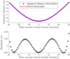 |
Fig. 1 Observation of a mutual approximation (i.e. close encounter between two natural satellites). The apparent distance between the two satellites (blue dots in the top panel) is frequently measured and a polynomial is used to fit these observationsand estimate the central instant of the close encounter (typically fourth-order polynomial, displayed in red). The residuals between the apparent distances measurements and the fitted polynomial are shown in black (bottom panel). |
2 Using mutual approximations in the estimation
In this section, we first provide a formal definition to describe the observation of a mutual approximation between two satellites in Sect. 2.1. We develop an analytical formulation for the central instants and their observation partials in Sects. 2.2 and 2.3, respectively. The light-time effect contribution to those partials is discussed in Sect. 2.4. Finally, the alternative mutual approximations’ observable (i.e. derivative of the apparent distance, as introduced in Sect. 1) is presented in more details in Sect. 2.5.
2.1 Mutual approximation definition
A mutual approximation involves an observer (denoted by the subscript O in the following), which is most commonly a ground station, and two natural satellites, between which a close encounter is observed (subscripts S1 and S2, respectively). Because the light has a finite speed, the time at which the mutual approximation is observed (observation time  ) differs from the time at which the light eventually received by the observer got reflected by each of the satellites (
 and
and  for satellites 1 and 2, respectively).
The relative range vectors between the satellites and the observer can thus be defined as follows (see Fig. 2):

The relative velocity and acceleration of the two satellites can then be expressed as

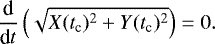
As mentioned in Sect. 1, a mutual approximation is defined as a point of closest encounter of two satellites in the field of view of an observer (see Fig. 1). This corresponds to the moment at which the apparent distance between the two moons reaches a minimum. The apparent distance as seen by an observer is
 (5)
(5)
where X and Y are the coordinates of the relative position between the satellites, in the instrumental frame of the observer.
The apparent relative position coordinates X and Y are defined as

X and Y thus depend on the right ascensions  and declinations
  of the two satellites, which are functions of the inertial relative range vectors with respect to the observer:

where ![Mathematical equation: $\left[x_{i},y_{i},z_{i}\right]$](/articles/aa/full_html/2021/08/aa41261-21/aa41261-21-eq11.png) correspond to the components of the relative range vectors
correspond to the components of the relative range vectors  (see Fig. 2). X and Y are thus time-dependent, as they are indirectly defined by the time-varying relative range vectors between each of the two satellites and the observer. In the rest of this paper, ri denotes the norm of these relative range vectors and
  the norm of the reduced vector
 ![Mathematical equation: $\left[x_{i},y_{i},0\right]$](/articles/aa/full_html/2021/08/aa41261-21/aa41261-21-eq14.png) . δm refers to the average declination, such that
. δm refers to the average declination, such that  . The differences in right ascension and declination are noted
  and
and 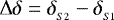 .
.
By definition, the central instant tc of a mutual approximation (recorded by the observer) fulfills the following condition:
 (10)
(10)
The apparent distance at tc is referred to as the impact parameter of the mutual approximation and denoted dc.
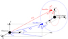 |
Fig. 2 Schematic representation of the different coordinate systems and positions. The first satellite and all associated notations are depicted in red, while blue is used for the second satellite.
|

![Mathematical equation: $\left[x_{i},y_{i},z_{i}\right]$](/articles/aa/full_html/2021/08/aa41261-21/aa41261-21-eq167.png)


![Mathematical equation: $\left[x^{\prime}_{i},y^{\prime}_{i},z^{\prime}_{i}\right]$](/articles/aa/full_html/2021/08/aa41261-21/aa41261-21-eq170.png)
![Mathematical equation: $\left[\boldsymbol{e}_{_r}^{S_i},\boldsymbol{e}_{_s}^{S_i},\boldsymbol{e}_{_w}^{S_i}\right]$](/articles/aa/full_html/2021/08/aa41261-21/aa41261-21-eq171.png)


2.2 Analytical expressions for central instants
The central instant tc is typically determined by fitting a fourth order polynomial to the apparent distance history between two satellites (see Fig. 1). The roots of the derivative of the fitted polynomial provide the estimated central instant of the close encounter. For simulated mutual approximations, the procedure can be iterated to improve the precision of the predicted central instants by re-centring the polynomial fit on the current estimate of the point of closest approach.
A fourth order polynomial is needed to reproduce the relative motion of the two satellites over the typical duration of a close encounter (i.e. 60 minutes). However, when focusing on only a fraction of this event, a fourth order polynomial is not necessary. For instance, a second order polynomial provides a fit over the interval 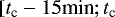
![Mathematical equation: $\left.+15\text{min}\right]$](/articles/aa/full_html/2021/08/aa41261-21/aa41261-21-eq20.png) which is as good as the one provided by a fourth order polynomial over the whole event, as shown in Appendix A.
which is as good as the one provided by a fourth order polynomial over the whole event, as shown in Appendix A.
To derive observation partials, we quantify the effect of very small changes in position and velocity of the two satellites. We are thus investigating only slight variations of the central instant tc, and can limit our analysis to short time intervals centred on the current estimate of tc. Consequently, for our analysis, it is safe to approximate the apparent relative motion of the two satellites by a second order polynomial only.
Around the point of closest approach, the relative position coordinates X and Y can thus be expressed as a function of three polynomial coefficients each:

These polynomial coefficients are directly given by the apparent relative position, velocity, and acceleration coordinates at central instant tc. Introducing the relative time t′ = t − tc as well as simplified notations (Xc = X(tc), Ẋc = Ẋ(tc), etc.), Eqs. (11) and (12) can be rewritten as follows:

The relative velocity coordinates are then approximated by a first order polynomial when close enough to the central instant:

Higher-order terms could be included in Eqs. (13)–(16). However, as discussed above, a second-order polynomial is well-suited to reproduce the apparent relative motion of the two satellites around the point of closest encounter. Higher-order terms can thus be safely neglected, as shown by the verification of our analytical partials for central instants (see Appendix D).
As already mentioned in Sect. 2.1, the derivative of the apparent distance is equal to zero at central instant tc. Therefore, the dot product between the relative position and velocity vectors must be equal to zero, leading to the following condition:
 (17)
(17)
The above equation can be rewritten as a third-order polynomial expression in t′:
 (18)
(18)
Solving for t′ is equivalent to finding the roots of this cubic polynomial, which can be done analytically with Cardano’s formula (e.g. Weisstein 2002). In case the cubic polynomial has three real roots, the closest to the current tc estimate should be selected, the other two falling outside the nominal duration of the close encounter event in most cases. An analytical expression can thus be derived for t′, as a function of the apparent position, velocity, and acceleration components at tc:
 (19)
(19)
Formulations for Ẋ and Ẏ are derived from expressions for X and Y (Eqs. (6) and (7)), as follows:

 and
and  can be computed from Eqs. (8) and (9) as a function of the inertial relative position and velocity:

Finally, the apparent relative acceleration components ẍ and Ÿ are required and can be similarly derived:

where the second time derivatives of α and δ also depend on the inertial relative acceleration:
![Mathematical equation: \begin{align}\ddot{\alpha}_{_{S_{i}}} &= \frac{-2\left(x_{i} \dot{y}_{i} - y_{i} \dot{x}_{i}\right)\left(x_{i} \dot{x}_{i} + y_{i} \dot{y}_{i}\right)}{r_{i_{xy}}^4} + \frac{\left(x_{i} \ddot{y}_{i} - y_{i} \ddot{x}_{i}\right)}{r_{i_{xy}}^2},\\\ddot{\delta}_{_{S_{i}}} &= \frac{1}{r_{i}^2 r_{i_{xy}}} \left[{\vphantom{\frac{2 \left(\boldsymbol{r}_{_O}^{S_{i}} \cdot \dot{\boldsymbol{r}}_{_O}^{S_{i}}\right)}{r_{i}^2}}} -z_{i} \left(x_{i}\ddot{x}_{i} + y_{i} \ddot{y}_{i}\right) + r_{i_{xy}}^2\ddot{z}_{i} \right. \nonumber \\&\quad\left.-z_{i} \frac{\left(x_{i} \dot{y}_{i} - y_{i} \dot{x}_{i}\right)^2}{r_{i_{xy}}^2}\right. \nonumber \\&\quad\left.+\frac{2 \left(\boldsymbol{r}_{_O}^{S_{i}} \cdot \dot{\boldsymbol{r}}_{_O}^{S_{i}}\right)}{r_{i}^2} \left(z_{i}(x_{i} \dot{x}_{i} + y_{i} \dot{y}_{i})- \dot{z}_{i}r_{i_{xy}}^2\right)\right]; i\in\{1,2\}.\end{align}](/articles/aa/full_html/2021/08/aa41261-21/aa41261-21-eq32.png)
Inserting Eqs. (8)–(9), (22)–(23), and 26–27 into Eqs. (6)–(7), (20)–(21), and (24)–(25) gives a direct analytical expression for t′, and therefore for the central instant tc, via Eq. (19).
2.3 Partials with respect to the natural satellites’ states
To estimateephemerides using central instants as observables, the partials of tc with respect to the states of the two natural satellites are required. Recalling the analytical expression obtained for t′ (Eq. (19)) and noting q the vector of parameters, the central instants partials are
![Mathematical equation: \begin{align*}\frac{\partial t^{\prime}}{\partial \boldsymbol{q}} = \,&\frac{\partial f\left(X_{\textrm{c}}, Y_{\textrm{c}}, \dot{X}_{\textrm{c}}, \dot{Y}_{\textrm{c}}, (((ddX)))_{\textrm{c}},(((ddY)))_{\textrm{c}}\right)}{\partial \boldsymbol{q}} \\= \,&\frac{\partial f}{\partial [X_{\textrm{c}},Y_{\textrm{c}}]}\frac{\partial [X_{\textrm{c}},Y_{\textrm{c}}]}{\partial \boldsymbol{q}} + \frac{\partial f}{\partial [\dot{X}_{\textrm{c}},\dot{Y}_{\textrm{c}}]}\frac{\partial [\dot{X}_{\textrm{c}},\dot{Y}_{\textrm{c}}]}{\partial \boldsymbol{q}} \nonumber \\&+ \frac{\partial f}{\partial [(((ddX)))_{\textrm{c}},(((ddY)))_{\textrm{c}}]}\frac{\partial [(((ddX)))_{\textrm{c}},(((ddY)))_{\textrm{c}}]}{\partial \boldsymbol{q}}.\end{align*}](/articles/aa/full_html/2021/08/aa41261-21/aa41261-21-eq33.png)
The partials of the relative apparent position, velocity, and acceleration can be decomposed as a function of the partials of  ,
,  ,
,  ,
,  ,
,  , and
, and  , as follows:
![Mathematical equation: \begin{align*}\frac{\partial \left[X,Y\right]}{\partial \boldsymbol{q}} = \;& \frac{\partial[X,Y]}{\partial \left[\alpha,\delta\right]_{_{S_{i}}}}\frac{\partial \left[\alpha, \delta \right]_{_{S_{i}}}}{\partial \boldsymbol{q}}, \\\frac{\partial [\dot{X},\dot{Y}]}{\partial \boldsymbol{q}} = \;& \frac{\partial[\dot{X},\dot{Y}]}{\partial \left[\alpha,\delta\right]_{_{S_{i}}}}\frac{\partial \left[\alpha,\delta\right]_{_{S_{i}}}}{\partial \boldsymbol{q}} +\frac{\partial[\dot{X},\dot{Y}]}{\partial [\dot{\alpha},\dot{\delta}]_{_{S_{i}}} }\frac{\partial[\dot{\alpha},\dot{\delta}]_{_{S_{i}}} }{\partial \boldsymbol{q}}, \\\frac{\partial \left[(((ddX))),(((ddY)))\right]}{\partial \boldsymbol{q}} = \;& \frac{\partial[(((ddX))),(((ddY)))]}{\partial [\alpha,\delta]_{_{S_{i}}}}\frac{\partial [\alpha,\delta]_{_{S_{i}}}}{\partial \boldsymbol{q}}+\frac{\partial[(((ddX))),(((ddY)))]}{\partial [\dot{\alpha},\dot{\delta}]_{_{S_{i}}}}\frac{\partial [\dot{\alpha},\dot{\delta}]_{_{S_{i}}} }{\partial \boldsymbol{q}} \nonumber \\&+\frac{\partial[(((ddX))),(((ddY)))]}{\partial [\ddot{\alpha},\ddot{\delta}]_{_{S_{i}}}}\frac{\partial [\ddot{\alpha},\ddot{\delta}]_{_{S_{i}}} }{\partial \boldsymbol{q}}; i\in\{1,2\}.\end{align*}](/articles/aa/full_html/2021/08/aa41261-21/aa41261-21-eq40.png)
From the definition of the apparent position (X,Y), velocity (Ẋ, Ẏ), and accelerations ẍ,Ÿ in Eqs. (6)–(7), (20)–(21), and (24)–(25), their partials with respectto the satellites’ states can be easily derived (the proof is left as an exercise to the reader). Finally, the partials of α, δ,  ,
,  ,
,  , and
, and  also need to be computed with respect to the position and velocity vectors of the two satellites.
To quantify the influence of the uncertainties in the observer’s state on the estimated solution, partials with respect to  and
and  might also be required. All derivations are provided in Appendix B. Our analytical formulation for the partials of the central instants with respect to both the satellites’ and observer’s states were validated numerically. The results of this verification are reported in Appendix D.
2.4 Light-time effects
In Sect. 2.3, the contribution of the light-time effects was not yet included in the observation partials and we therefore assumed that both  and
and  were fixed. Corrections required to account for the finite speed of light are now discussed.
When computing light-time effects, we typically fix either the time at the observed body (here  ) or the time at the observer (
 ). The other one is determined via an iterative scheme to ensure that the difference between the two times matches the light-time calculated from the observer and observed bodies’ states (Moyer 2000). For mutual approximations, the reception time should always be fixed. Fixing the two transmission times would indeed lead to two different inconsistent reception times for a unique observation. The light-time equations are expressed as follows (Moyer 2000):
 (33)
(33)
where c refers to the speed of light and the observation time tO is a fixed unique value.
The partials of the light-time with respect to a vector of parameters q can then be derived from Eq. (33):
 (34)
(34)
Solving for the partials of  with respect to q, we finally obtain (Moyer 2000)
 (35)
(35)
The time  thus depends on both the natural satellite’s and observer’s states. As already mentioned, right ascension and declination partials with respect to the vector of parameters q were provided for fixed
  and
and  in Sect. 2.3. When accounting for the light-time effect, the complete formulation for those partials becomes
![Mathematical equation: \begin{align*}\frac{\partial \left[\alpha,\delta\right]_{_{S_{i}}}}{\partial \boldsymbol{q}} &= \left.\frac{\partial \left[\alpha,\delta\right]_{_{S_{i}}}}{\partial \boldsymbol{q}}\right|_{t_{_{Si}}}+\left[\dot{\alpha},\dot{\delta}\right]_{_{S_{i}}}\frac{\partial t_{_{Si}}}{\partial \boldsymbol{q}}; \text{ } i\in \{1,2\}.\end{align*}](/articles/aa/full_html/2021/08/aa41261-21/aa41261-21-eq58.png) (36)
(36)
The same applies to the partials of  ,
,  ,
,  , and
, and  , and leads to the following expressions:
![Mathematical equation: \begin{align*}\frac{\partial [\dot{\alpha},\dot{\delta}]_{_{S_{i}}}}{\partial \boldsymbol{q}} &= \left.\frac{\partial [\dot{\alpha},\dot{\delta}]_{_{S_{i}}}}{\partial \boldsymbol{q}}\right|_{t_{_{Si}}}+[\ddot{\alpha},\ddot{\delta}]_{_{S_{i}}}\frac{\partial t_{_{Si}}}{\partial \boldsymbol{q}}, \\\frac{\partial [\ddot{\alpha},\ddot{\delta}]_{_{S_{i}}}}{\partial \boldsymbol{q}} &= \left.\frac{\partial [\ddot{\alpha},\ddot{\delta}]_{_{S_{i}}}}{\partial \boldsymbol{q}}\right|_{t_{_{Si}}}+[\dddot{\alpha},\dddot{\delta}]_{_{S_{i}}}\frac{\partial t_{_{Si}}}{\partial \boldsymbol{q}}; \text{ } i\in \{1,2\}.\end{align*}](/articles/aa/full_html/2021/08/aa41261-21/aa41261-21-eq63.png)
According to Eq. (38), the complete partials for  and
and  require one to compute
  and
and  (see Eq. (38)), and thus the time derivative of the relative acceleration of each satellite with respect to the observer. This would significantly increase both the implementation and computational efforts, while the
  and
and  partials only marginally contribute to the central instant partials (at most of the order of 0.001% for the case of the Galilean satellites, see Table E.1). As a consequence, neglecting the light-time effects when computing the partials for
  and
and  is a fair simplifying assumption, which was applied in the rest of this study.
2.5 Alternative observables
As already mentioned in Sect. 1, the alternative observable recommended by Morgado et al. (2019) correspond to the derivative of the apparent distance, defined as
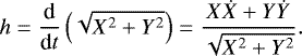 (39)
(39)
If X and Y and their time derivatives Ẋ and Ẏ were computed at the exact central instant tc of the close encounter, the observable h would by definition be equal to zero. This is however not the case. This observable thus indirectly evaluates the difference between the current estimate of tc and its true value by quantifying how much the derivative of the apparent distance departs from zero.
In contrast to central instants which also depend on the satellites’ relative accelerations, alternative observables are thus only a function of their relative position and velocity. The partials of such an observable with respect to a vector of parameters q are much easier to derive than for central instants and are given by Morgado et al. (2019):
 (40)
(40)
The results of the comparison between the two types of observables are discussed in Sect. 4.
3 Observations simulation and ephemerides estimation
We first describe how mutual approximations are simulated in Sect. 3.1, before introducing the covariance analysis used to compare the two observable types in Sect. 3.2. The strategy applied to weight the mutual approximations’ observables is then discussed in Sect. 3.3. Finally, Sect. 3.4 defines an additional figure of merit to analyse the estimation solution.
3.1 Mutual approximations simulation
We used simulated mutual approximations in our analysis. As a preliminary test case, we first propagated the trajectories of Io and Europa only and detected close encounters between these two moons (results discussed in Sects. 4.1 to 4.4). A more complete simulation including all Galilean moons was also conducted to verify the findings of the former simple test case (Sect. 4.5).
The orbits of the Galilean moons were propagated using a simplified dynamical model. For each of the moons, we considered only the point-mass gravitational accelerations exerted by Jupiter and the three other satellites. A more detailed dynamical model (e.g. Dirkx et al. 2016; Lainey et al. 2004) would yield more accurate propagated orbits for the Galilean moons, and thus affect the predicted mutual approximations. However, we focus on comparing two types of mutual approximations’ observables. High-accuracy dynamical modelling is therefore not critical for this study, as long as the same set of simulated observations is used for both observable types.
Mutual approximations were simulated for the period 2020–2029. To limit the number of observations, we only considered mutual approximations with an impact parameter lower than 30 arcseconds (as), in accordance with Morgado et al. (2019). We selected three of the ground stations involved in the 2016–2018 observational campaign reported in Morgado et al. (2019), designated by FOZ, OHP, and OPD (their coordinates are reported in Table 1). To ensure the feasibility of the observation, events which would be observable during daytime were discarded. In addition, the lower limit on the distance between the mutual approximation and the limb of Jupiter was set to 10 as. Only mutual approximations that would be observed from the three ground stations under an elevation angle larger than 30 degrees were included.
When achievable under the aforementioned conditions, a single event can be observed by several ground stations. Those multiple observations of one mutual approximation were assumed to have uncorrelated noise and thus they were added as independentobservations to the state estimation. This implies that such simultaneous observations improve the estimation solution by increasing the size of the observational data set, as formal errors are expected to scale down with  (n being the total number of observations).
Finally, weather conditions were taken into account to obtain a realistic set of observations. Due to bad weather conditions, about 35% of the predicted mutual approximations could not be observed during the 2016–2018 campaign (Morgado et al. 2019). We took a conservative approach to simulate these bad weather conditions and discarded 50% of the viable observations, selected arbitrarily using a uniform distribution.
The distribution per year of the remaining simulated mutual approximations is shown in Fig. 3. Figure 3a displays the fraction of simulated events per ground station, while Fig. 3b focuses on the number of mutual approximations for each combination of two Galilean moons. It is interesting to note that no mutual approximation respecting the conditions mentioned in the previous paragraphs could be found in 2020, and that some years are more favourable to such events, due to the time evolution of the Earth–Jovian system relative geometry.
Ground stations’ geodetic coordinates.
3.2 Covariance analysis
To compare state estimations obtained with the two types of mutual approximation observables, we limited ourselves to a covariance analysis. Despite its limitations (Gaussian observation noise, dynamical and observational models assumed perfect), such an analysis is well-adapted for comparison purposes. Formal errors are known to be too optimistic compared to true errors, but we only focus on comparing two sets of estimation errors and not on absolute error values. Since mutual approximations are almost exclusively sensitive to the relative dynamics between the two satellites while both their absolute states are estimated, realistic errors are anyway difficult to achieve without including other observations.
In our simulations, the estimated parameters were the initial states of the moons involved in the mutual approximations. In most of our analysis, only the Jupiter-centred initial states of Io and Europa are estimated (Sects. 4.1 to 4.4), while we also solved for the initial states of Ganymede and Callisto in the more complete case used for verification (see Sect. 4.5). For the moons’ initial position components, a priori covariance of 100 km was considered, while it was set to 100 m s−1 for their initial velocity. These a priori values are large, but were only included to slightly constrain the estimation, thus avoiding an ill-posed problem and making the comparison between the two observable types’ estimation solutions possible.
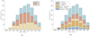 |
Fig. 3 Distribution of the simulated mutual approximations per year, depending on the ground station (panel a) and on the two moons involved (panel b). Mutual approximations which have been discarded to mimic the effect of bad weather conditions are not included in this distribution. |
3.3 Data weights
Observation weights are usually applied to account for the quality of the data. For our comparative analysis, it is essential to ensure that the data weights are consistent between the two types of observables. We used an error of 3.5 s for the central instants tc (average error obtained over the 104 observed mutual approximations of the 2016–2018 campaign reported in Morgado et al. 2019).
To derive appropriate weights for the alternative observables, the shape of the simulated mutual approximation must be taken into account. By definition, the derivative of the apparent distance (i.e. alternative observable) is always equal to zero at t = tc. However, an error of 3.5 s in the determination of the central instant would shift this value away from zero. The exact value of the resulting alternative observable error directly depends on the specific geometry of each mutual approximation. The alternative observable error was thus individually computed for each observation, as follows:
 (41)
(41)
where  is set to its averaged value (
 s) and ḋ is the derivative of the apparent distance (given by Eq. (39)).
Consistent weights between the two observables are not only needed to perform a meaningful comparison. When using alternative observables, weighting can be an indirect way to account for the satellites’ relative dynamics during the close encounter. Indeed, a non-zero value for the derivative of the apparent distance at tc only quantifies how much the observed central instant departs from the current point of closest approach. However, it does not provide any information about the current apparent distance minimum. For a given non-zero value of the apparent distance derivative, the difference between the observed and current central instants entirely depends on the satellites’ apparent relative dynamics, which drive the geometry of the observed encounter.
This effect is, by definition, inherently captured by central instants, for which applying an appropriate constant weight value is thus suitable. For alternative observables, on the other hand, individual weights accounting for each mutual approximation’s dynamics, as given in Eq. (41), are crucial. This is necessary to translate an error in the estimated central instant to an error in the derivative of the apparent distance.
The importance of applying this weighting strategy to obtain consistent estimation solutions with the two different observable types is demonstrated in Sect. 4.4. Furthermore, we computed the appropriate alternative observables’ weights for the past mutual approximations observed during the 2016–2018 campaign and reported in Morgado et al. (2019). These weights are providedin Appendix F and should be used when including the 2016–2018 mutual approximations in the state estimation.
3.4 Contribution of each observation to the solution
To perform a detailed comparison of the two observable types, mutual approximations’ contributions to the solution were used as an additional figure of merit to complement the covariance analysis. In this study, each observation’s contribution to the solution is defined asthe root-mean-square (RMS) of the weighted observation partial with respect to the parameters of interest’s vector q.
For example, the contribution c of an observation h to Io’s Jupiter-centred initial position vector is expressed as:
 (42)
(42)
where t0 is the initial epoch at which Io’s state is estimated. The contribution  to the vector of parameters q is then normalised as follows (the bar indicates normalisation):
 (43)
(43)
where  is the vector containing the contributions of the entire set of mutual approximations with respect to q (for one type of observable).
 |
Fig. 4 Time evolution of the formal errors in Io’s and Europa’s initial RSW coordinates (radial, normal, and axial directions, see Fig. 2), as more observations are progressively included in the state estimation. The blue line displays the time evolution of the formal errors obtained by using the central instants as observables (left y-axis). The red line corresponds to the time evolution of the formal errors obtained from alternative observables (left y-axis too). The initial values of the formal errors, before including any observation, correspond to the a priori covariance values used for the regularisation (i.e. 100 km, see Sect. 3.2). The grey line (right y-axis) represents the relative difference (in percentage) between the two solutions as a function of time. The formal errors are equal to their initial values until the inclusion of the first mutual approximation (towards the end of 2021) and no difference between the two observables’ solutions is thus observed beforehand. |
4 Results
We present here the results of the comparison between the ephemeris estimation determination solutions obtained using central instants andalternative observables, respectively. The comparison is first conducted for a simple test case with Io and Europa only, to analyse how each mutual approximation contributes to the ephemerides solution and how this affects the relative performanceof the two types of observables. Results of this first analysis are presented in Sects. 4.1 to 4.4. A more complete test case also including Ganymede and Callisto is used to verify those findings (Sect. 4.5).
4.1 Comparison over the 2020–2029 observational period
We first only simulated mutual approximations between the two innermost Galilean moons, for the period 2020–2029, and estimated Io’s and Europa’s initial states from those simulated observations. The evolution of the formal errors with time is displayed in Fig. 4, as more mutual approximations are included in the estimation. The differences in formal errors between the two types of observables do not exceed 20% at the end of our simulation, after 10 yr of observations. Alternative observables and central instants lead to comparable formal errors evolutions. At first order, this proves that the two types of mutual approximations’ observables are largely equivalent, at least when enough observations are added to the state estimation. It validates the recommendations formulated in Morgado et al. (2019), but seems to contradict the results on numerical partials in Emelyanov (2017).
Nonetheless, using central instants still results in slightly lower formal errors for each component of both Io’s and Europa’s initial position. The formal error improvement is stronger in the radial and normal directions (about 20% for both Io and Europa at the end of simulation) and less significant in the axial direction (only 10–12%). As mentioned in Sect. 2.5, the observation partials developed for the central instants account for variations in the apparent relative acceleration between the two satellites, while this is not the case for alternative observables. The additional information captured by central instants thus principally lies within the orbital plane of theGalilean moons, within which the inter-moons accelerations primarily lie. On the other hand, the central instants are not significantly more sensitive than alternative observables to state variations in the axial direction.
Interestingly, the difference in formal errors between the two types of observables is not constant over time, as clearly highlighted by Fig. 4. It can be as low as a few percents (e.g. Io’s normal position in year 2021) or as high as 35% (e.g. Io’s normal position during the first half of year 2027). This is related to the mutual approximations’ heterogeneous contribution to the solution: it varies from one observation to another, but also between thetwo observable types. The cause of this heterogeneity is further discussed in Sect. 4.2.
First, as expected, the contribution of each mutual approximation depends on the time at which it occurs. Observations collected further in time (with respect to the initial epoch t0 at which the states are estimated) indeed contribute more to the initial state solution. This directly results from the fact that later observationsprovide tighter constraints to the initial state due to the orbit propagation: the effect of a slight variation in the initial state of Io and Europa on their trajectories grows with time. However, this time trend similarly affects both observable types and thus it has no noticeable influence on the solution improvement provided by central instants.
Nonetheless, the observable type choice also has an effect on some mutual approximations’ contribution to the estimated solution. Figure 5 displays the normalised contribution ratio of central instants over alternative observables, as defined in Sect. 3.4, for each mutual approximation. Some mutual approximations, mostly concentrated in the 2026–2027 period, contribute significantly less to both Io’s and Europa’s estimated positions when alternative observables are used instead of central instants. As expected, these observations coincide with an increase of the difference in formal errors between the two observables. The coming sections investigate why this discrepancy between the two observable types only concerns some mutual approximations and specific observational periods.
 |
Fig. 5 Reduction in formal errors obtained by using central instants instead of alternative observables, as more observations are added to the solution. It is displayed on the left axis, for the three position components in RSW frame (panel a: Io, panel b: Europa). On the right axis (purple dots), the ratio between the normalised contributions of central instants over their corresponding alternative observables is displayed, for each mutual approximation (normalised contributions are computed as in Eq. (43)). As mentioned in Sect. 3.1, the first simulated observation only occurs towards the end of 2021, hence the lack of data beforehand. |
 |
Fig. 6 Observations’ contributions to the estimated initial positions’ solution (in colours), as a function of each mutual approximation’s characteristics (impact parameters and impact velocities, reported on the x- and y-axes, respectively). Panel a: normalised contribution of each mutual approximation to the solution (averaged between Io and Europa), when using central instants. Panel b: ratio between the normalised contributions of central instants over their corresponding alternative observables. The normalised contribution of each mutual approximation to the solution is obtained with Eq. (43). |
4.2 Influence of the mutual approximations’ characteristics
To better characterise the difference between the two observable types, we further analyse the relative contribution of each observation and the effect of the mutual approximation’s characteristics. Section 4.2.1 discusses the influence of the impact parameter and velocity on each mutual approximation’s contribution to the solution, for both central instants and alternative observables. The link between those characteristics and the observation geometry is explored in Sect. 4.2.2.
4.2.1 Influence of impact parameter and velocity on each mutual approximation’s contribution
Focusing on the central instants case first, Fig. 6a shows that each mutual approximation’s contribution to the estimated positions (averaged between Io and Europa) strongly depends on the impact parameter and velocity. Highest contributions are systematically obtained with both low impact parameter and velocity (up to about 7 as and 1 mas s−1, respectively). Mutual approximations with either low impact parameter and high impact velocity, or high impact parameter but low impact velocity also contribute significantly to the ephemerides solution.
Using alternative observables instead of central instants alters the way some mutual approximations contribute to the estimated solution, as hinted in Sect. 4.1. Figure 6b displays the ratio between central instants’ and alternative observables’ contributions to the estimated initial positions (contributions were again averaged between Io and Europa). Mutual approximations characterised by low impact parameter and high impact velocity contribute significantly less to the solution when switching to alternative observables. More precisely, most mutual approximations with impact parameters lower than 5 as and impact velocities larger than 4 mas s−1 contribute about 2 times more to the estimated solution when using central instants instead of alternative observables.
This analysis proves that the differences between the two observable types for some mutual approximations is amplified by specific impact characteristics. Furthermore, mutual approximations identified as unfavourable for alternative observables (low impact parameters with large impact velocities) are not evenly distributed over the 2020–2029 observational period, but rather concentrated in the 2026–2027 interval. As expected, it corresponds to the period during which the differences in formal errors between the two observables increase (Sect. 4.1, see Fig. 5).
It is interesting to note that mutual approximations characterised by extremely low impact parameters are also unfavourable from an observational perspective, and not only from an estimation point of view. If the two satellites eventually become so close that a (partial) occultation occurs, the observer cannot distinguish between their images anymore, introducing a gap in the apparent distance measurements near the point of closest approach and thus leading to a larger error in the estimated central instant (Morgado et al. 2019).
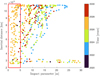 |
Fig. 7 Effect of the inertial geometry on the mutual approximations’ impact characteristics. Both the impact parameter and the inertial distance between Io and Europa (as opposed to apparent distance as seen from the ground stations) are displayed, for each mutual approximation. The colours represent the time at which the observation is made. |
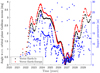 |
Fig. 8 Effect of the observation geometry on the mutual approximations’ impact parameters. The angle between the orbital plane of the Galilean moons and the observation vectors (Earth-Io in black and Earth-Europa in red) is plotted for each mutual approximation. The corresponding impact parameters (in as) are represented by blue dots. |
4.2.2 Link to the observation geometry
Interestingly, most of the mutual approximations simulated over the 2026–2027 period are characterised by low impact parameters (lower than 5 as), while it is not the case outside of this time interval. This is clearly shown in Fig. 8, where impact parameters are displayed in blue.
The apparent relative motion of the two moons is driven by two parameters: their inertial relative motion in the Jovian system and the observation geometry. Figure 7 focuses on the former and shows the absolute distance between Io and Europa for each mutual approximation, as a function of the corresponding impact parameter. The time at which each mutual approximation occurs is displayed in colours. When excluding the 2026–2027 interval (orange dots), the impact parameters take a wide range of values (up to the limit of 30 as). The lowest impact parameters usually coincide with low inertial distances between Io and Europa, typically below 3.5 × 10⁵ km (see the fraction of Fig. 7 highlighted in red). It should be noted that the reverse is not true: low inertial distances do not automatically lead to low impact parameters.
However, during the 2026–2027 period, mutual approximations with low impact parameters are systematically achieved, even for large inertial distances between Io and Europa. This difference between the inertial and apparent relative motions is caused by the evolution of the observation geometry. Figure 8 displays the angle between theorbital plane of the Galilean moons and the two observation vectors (Earth-Io and Earth-Europa), for each mutual approximation. The 2026–2027 period coincides with an almost perfect alignment between the satellite-observer vectors and the moons’ orbital plane, resulting in overall lower apparent distances during Io-Europa close encounters. Those low impact parameters then regularly happen to be combined with large impact velocities. This is why mutual approximations with both aforementioned characteristics, for which the differences between the two observable types are the largest (see Sect. 4.2.1), mostly occurred during years 2026 and 2027.
Such an observational period is thus not a special isolated case, but rather a periodic effect of the Earth–Jovian system geometry. Therefore, mutual approximations less favourable to alternative observables are expected to occur repeatedly, about every 6 yr, and coincide with the so-called ‘mutual events season’ during which eclipses and occultations occur. Implications of this effect of the observation geometry concerning the selection of the appropriate mutual approximations’ observable type are discussed in Sect. 4.3.
It must be stressed that the selected weighting strategy for alternative observables (Sect. 3.3) accounts for the mutual approximation’s characteristics and thus indirectly for the close encounter’s geometry. The aforementioned impact of the observation geometry on the equivalence between the two observable types and more precisely on the benefit of using central instants over alternative observables is therefore already attenuated by our careful weighting of the latter. Section 4.4 investigates the consequences of this geometry effect when not taken into consideration in the observation weights.
4.2.3 Observational period reduced to 2026–2027
To quantify the impact of using a limited observation set when it unfortunately corresponds to the observational period less favourable to alternative observables, we ran additional simulations including only 2026–2027 mutual approximations in the state estimation. Table 2 compares the improvement in formal errors provided by central instants over alternative observables with either complete (2020–2029) or partial (2026–2027) observation sets.
As expected, the differences in formal errors between the two observables increase when only considering 2026–2027 observations, except for Europa’s axial position component. The improvement provided by central instants is multiplied by factors ranging from 1.5 to 3 for most position and velocity components. Compared to results obtained with the complete observation set, formal errors’ improvements in the axial direction become more significant. They are even comparable to those achieved in the radial direction for both Io’s and Europa’s velocity.
Although alternative observables and central instants were proven to lead to very comparable solutions in nominal configurations, the influence of the available set of observations must thus not be neglected. If the number of mutual approximations is limited, or the period over which they were observed too short, it is recommended to investigate the characteristics of the available mutual approximations before selecting an observable type. The improvement provided by using central instants is indeed amplified when exclusively including mutual approximations observed under unfavourable observation angles (2026–2027 period in our case).
4.3 Implications
If enough observations are available, the improvement provided by using central instants instead of alternative observables is limited to about 20% for our Io-Europa test case. However, such improvement might still be relevant when concurrently estimating other dynamical parameters along with natural bodies’ ephemerides. Accurate determination of the tidal dissipation, in particular, is required to gain insights into the orbital evolution of planetary systems.
Recent estimations from astrometric data indeed showed that Saturn’s tidal quality factor Q can vary by several orders of magnitude from one moon’s forcing frequency to another (Lainey et al. 2020). These results are highly inconsistent with current evolution models and thus they highlight the need for accurate frequency-dependent estimation of tidal parameters (Fuller et al. 2016). This is for instance not yet done for Jupiter, whose tidal quality factor is currently only determined at Io’s frequency. A 20% improvement in the formal errors of the natural satellites’ initial states might be critical for such applications. As many perturbing dynamical effects can be absorbed by a variation in the initial state,any improvement in the state estimation can indeed help to detect and estimate such small tidal effects.
Furthermore, a 20% improvement in the predicted position and/or velocity of the targeted body is not negligible for orbital design applications. It can indeed affect the corrective manoeuvres required before and after a flyby or an orbital insertion, allowing for a more efficient design and thus reducing the ΔV budget.
The impact of the mutual approximations’ observables choice then depends on the timing of the manoeuvre. Figure 9 displays the improvement in propagated errors in radial, normal, and axial direction for both Io’s and Europa’s positions. The 20% difference in the formal errors of the initial states can increase once propagated, at least in the radial and normal directions. Depending on the time at which the manoeuvre is planned, the improvement in the accuracy of the predicted targeted body’s state might thus be higher than 20% if central instants are used. Looking at Fig. 9a, differences can reach up to 35% for Io’s radial and normal position components while they increase up to almost 40% for Europa (see Fig. 9b).
For Europa, the largest differences in propagated errors clearly correspond to the 2026–2027 period and thus coincide with the least favourable observation geometry for alternative observables (see discussion in Sect. 4.2). This effect is however barely noticeable in Fig. 9a, for Io’s case. Yet, it should be pointed that when a very sensitive manoeuvre is planned during such a particular observational period, the impact of the observable choice on the quality of the estimated solution might not be negligible.
All aforementioned points are direct consequences of the imperfect equivalence between the two types of observables, which might be accentuated when fewer observations are available. In practice, however, this would be balanced by other observations combined with mutual approximations in the state estimation. Building on Sect. 4.2, it is nonetheless worth highlighting that the number and distribution of the observations should be carefully considered when selecting an appropriate observable for the processing of mutual approximations data.
The fact that the alternative observables’ unfavourable observational period corresponds to the mutual events season might also be an interesting finding for the processing of the mutual events themselves. Indeed, if the timings at which eclipses and occultations occur were to be directly used as observables (as it is the case with mutual approximations’ central instants), the aforementioned effect of the observation geometry would first need to be carefully investigated.
Improvements in the final errors obtained with central instants, using two different observations sets.
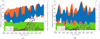 |
Fig. 9 Propagated formal errors in position components over the observational period (panel a: Io, panel b: Europa). The errors in position are expressed in the RSW frame (see Fig. 2) and are obtained from the propagated covariance matrix and estimated initial states. The purple dots (right axis) display the ratio between the normalised contributions of central instants over their corresponding alternative observables, for each mutual approximation. |
4.4 Influence of the weighting scheme
When enough mutual approximations are available, the good match which can be achieved between both observable types’ estimated solutions actually strongly depends on the accurate weighting of each mutual approximation. As highlighted in Sect. 3.3, individual weights have to be computed for alternative observables. Using a single averaged value for alternative observables’ weights yields a much larger discrepancy with respect to the central instants solution over the full simulation, as reported in Table 3. Compared to formal errors obtained with alternative observables, those achieved with central instants are then reduced by a factor 1.5 to 2.7 for the initial position components, and up to a factor 4 for the velocity components.
These results clearly prove that the equivalence between the two observable types is conditioned by the appropriate weighting of alternative observables. As mentioned in Sect. 3.3, it is crucial to carefully compute suitable observation weights to ensure that the alternative observables indirectly take into account the geometry of the close encounter in the plane of the sky.
Emelyanov (2017) already conducted a comparative analysis between the two types of observables, although the central instant partials were computed numerically. Interestingly, a convergence issue was encountered with alternative observables, while none was reported for central instants. This indicates that the two observables types were not perfectly equivalent in this case, which might be due to the weighting issue we just highlighted.
Comparison of the final formal errors obtained with the two types of observables, when applying constant weight values.
4.5 Verification case: four galilean moons
As verification, we simulated mutual approximations between the four Galilean moons of Jupiter. Ganymede’s and Callisto’s initial stateswere then estimated in addition to Io’s and Europa’s. The resulting formal errors in the four moons’ initial states are provided in Table 4. Even if not displayed here, the time evolution of the errors in Io’s and Europa’s initial states show a behaviour comparable to what was observed in the first test case limited to Io and Europa only (see Fig. 4). The final formal errors are however a bit lower in the four moons’ case.
Similarly to the Io-Europa test case, using central instants over alternative observables mostly improves errors in the radial and normal directions, but only has a marginal effect on the axial direction errors. For Europa’s axial position, the estimation is even 2% better with alternative observables. As shown in Table 4, differences in formal errors between thetwo types of observables are significantly lower for Callisto than for the three other moons. These differences are only of a few percents, while they reach about 10% for Io’s, Europa’s, and Ganymede’s initial positions.
Again, the contribution of each mutual approximation to the estimated ephemerides solution also reflects the higher sensitivity of central instants to the complex dynamics at play in the Jovian system. Figure 10 shows the contributionof every observation to the initial position of Io (blue), Europa (orange), Ganymede (green), and Callisto (purple). As expected, all mutual approximations contribute to estimating the initial states of Io, Europa, and Ganymede because of the Laplace resonance between these three moons. On the other hand, only mutual approximations directly involving Callisto significantly help to determine its initial state.
In Fig. 10, clear periodic patterns can be identified in the central instants case, at least when enough observationsare available, such as for Io-Europa, Io-Ganymede, and Europa-Ganymede mutual approximations. While still present, those patterns are however less pronounced for the alternative observables case. They are directly related to the relative motion of the satellites in the Jovian system (inertial motion, as opposed to apparent). This again indicates that part of the information encoded in mutual approximations is not fully captured by alternative observables.
As already highlighted by the Io-Europa case (Sect. 4.1), central instants are indeed more sensitive to the apparent relative acceleration between the two satellites. Central instants’ partials directly account for any acceleration variation induced by a small change in initial states, while alternative observables do not. This may also explain why differences between the two observables are lower for Callisto. As it is the most remote moon with respect to Jupiter, the distance between Callisto and each of the three other moons is larger than the distances between Io, Europa, and Ganymede, resulting in smaller inter-moon accelerations. Furthermore, because of the Laplace resonance between the three innermost Galilean satellites, accelerations exerted by one of these three moons on the other two strongly influence their dynamics. These two combined effects might strengthen the advantage of central instants over alternative observables for Io, Europa, and Ganymede, compared to Callisto.
Overall, all findings obtained in the first simple Io-Europa test case are confirmed by this second analysis extended to the four Galilean moons. The two types of observables lead to almost equivalent solutions if the alternative observables are properly weighted (see Sect. 3.3), despite a 10% reduction of the formal errors in both radial and normal directions when using central instants. The effect of the observation geometry is also similar to the Io-Europa case: low impact parameter, large impact velocity mutual approximations simulated in 2026–2027 are unfavourable to alternative observables.
Comparison of the formal errors in the initial positions of the four Galilean moons.
5 Conclusion and discussion
We developed an analytical formulation for the observation partials of the mutual approximations’ central instants. This allows those central instants to be directly used as observables to estimate the ephemerides of natural satellites. Our analytical method relies on a second-order polynomial to approximate the relative motion of two satellites around their point of closest approach. From this polynomial function, we derived an expression for the central instant as a function of the apparent relative position, velocity, and acceleration of the two satellites.
Higher-order terms could theoretically be included in our formulation. Using a third-order polynomial to reproduce the apparent relative motion of the two moons (Eqs. (11)–(12)) would lead to a fourth-order polynomial for the central instant (Eq. (18)). The roots of such a polynomial could still be computed analytically, but at the cost of a dramatic increase in complexity. However, a second-order polynomial has been proven sufficient to capture the apparent relative dynamics of the two satellites around their closest encounter and to yield highly accurate analytical partials for central instants.
Numerically computing partials for central instants is extremely computationally demanding (Emelyanov 2017). It requires to independently propagate small variations in each of the estimated parameters (at least six initial state components for each of the two moons involved). Afterwards, the new central instants must be determined, which is a time-consuming process in itself. Should central instants be used, our analytical approach is thus significantly faster than the numerical computation of the observation partials.
We conducted a comparative covariance analysis using either only central instants, or only mutual approximation’s alternative observables to estimate the Galilean moons’ ephemerides. When using the entire set of viable mutual approximations over the period 2020–2029, the difference in formal errors does not exceed 20% between the two types of observables. The central instants achieve the best ephemerides solution because alternative observables do not account for some of the dynamical effects affecting the close encounter (e.g. apparent relative acceleration between the two satellites). In contrast, these effects are directly captured by central instants, which is beneficial for the resulting estimated solution.
Overall, we still prove alternative observables to be almost equivalent to central instants, but only under specific conditions. First, when using alternative observables, the shape of the observed close encounter must indirectly be accounted for in the calculation of the observation weights, while it is automatically included in the central instant case. Individual and accurate weighting of each event, based on the apparent relative dynamics of the satellites, is then crucial to obtain a consistent solution. It is indeed necessary to convert any error in the estimated central instant to an error in the derivative of the apparent distance. We show that when using a single averaged value to weight all mutual approximations, the formal errors in initial states obtained with central instants were 1.5 to 4 times lower than with alternative observables in our test case. As discussed in Sect. 4.4, an inappropriate weighting scheme could thus possibly explain previous indications of a non-equivalence between the two observable types (Emelyanov 2017). When using alternative observables, we therefore recommend to adopt the weighting strategy described in Sect. 3.3, and more precisely to compute the weights with Eq. (41). In Appendix F, we provide the appropriate alternative observables’ weights for the 2016–2018 mutual approximations reported in Morgado et al. (2019). These weight values should be applied for the 2016–2018 observations to be properly included in the state estimation.
Furthermore, all mutual approximations do not homogeneously contribute to the ephemerides solution. The satellites’ dynamics are overall better constrained by mutual approximations with a low impact parameter (typically below 7 as) and low relative velocity (1 mas s−1), for both observable types. However, some characteristics in particular are unfavourable to alternative observables: mutual approximations with low impact parameters but large impact velocities contribute significantly more to the estimated solution when using central instants (factor 2 to 3). Preferring central instants is thus particularly advantageous for these specific mutual approximations, which are not isolated events but periodically represent most of the observations for 1 or 2 yr (see discussion in Sect. 4.2.2).
Choosing between the two types of observables when estimating ephemerides from mutual approximations therefore requires critical evaluation. If many mutual approximations are available to estimate the moons’ ephemerides, one can safely use alternative observables without substantially degrading the solution. However, this does not systematically hold for a small set of observations, especially if they are all collected during the alternative observables’ unfavourable observation period. The formal error reduction provided by our method then strongly depends on the mutual approximations’ characteristics.
The relevance of selecting central instants over alternative observables eventually depends on the application of the ephemeridessolution. As detailed in Sect. 4.3, a 10–20% improvement in the formal errors of the satellites’ state might be significant when concurrently estimating tidal parameters. It may also be non-negligible for mission design applications. Improved ephemerides are indeed crucial to design efficient flybys or orbital insertions requiring only limited corrective manoeuvres. The timing of the manoeuvres must then be taken into consideration to select a suitable observable, especially if they coincide with observation geometries less favourable to alternative observables.
As mentioned in Sect. 4.3, a comparable analysis could be conducted for mutual events. We expect to obtain consistent results with respect to the mutual approximations’ case, given the similarities between the two types of observation. However, allmutual events occur during the alternative observables’ unfavourable observational period. It is thus important to confirm the influence of the observation geometry on the differences between central instants’ and alternative observables’ state estimation solutions. This could be an interesting result, in case the timings of eclipses and occultations would be directly used as observables, as for mutual approximations.
 |
Fig. 10 Normalised contribution of mutual approximations between Io and Europa (I-E, left plots), Io and Ganymede (I-G, centre-left plots), Io and Callisto (I-C, centre-right plots), Europa and Ganymede (E-G, right plots) to the initial position of Io (blue), Europa (orange), Ganymede (green), and Callisto (purple). Results for Europa-Callisto and Ganymede-Callisto mutual approximations are not represented here, but do not show any trend that is not already highlighted by the contributions of the other observations. The first simulated observation only happens at the end of year 2021, explaining the lack of data before that date. |
Acknowledgements
We would like to thank Wouter van der Wal for his useful feedback, which significantly improved the quality of this manuscript.
Appendix A Fitting apolynomial to a close encounter’s apparent distance history
 |
Fig. A.1 Apparent distance measurements during a mutual approximation (blue dots on top panels). The polynomial used to fit these observations is typically a fourth order one (left panel). A second order polynomial was also tested, for the whole duration of the event (middle panels) and over a reduced time interval (30 min) centred on the central instant tc. For each of the three case, the residuals between the fitted polynomial and the true apparent distance history are displayed in the bottom panels. |
As described in Sect. 1, the apparent distance history during a close encounter between the two satellites is typically fitted with a fourth order polynomial (e.g. Morgado et al. 2016). This allows to estimate the mutual approximation’s central instant, as well as its impact parameter for instance. In this appendix, we discuss the influence of the order of the fitting polynomial. The maximum absolute values of the residuals between the fitted polynomial and the true apparent distance history are reported in Table A.1 (for the first mutual approximations predicted between Io and Europa, starting from 01/01/2020). For clarity, the apparent distance observations, fitted polynomial and resulting residuals are displayed in Fig. A.1 for the first mutual approximation.
When switching from a fourth order to a second order polynomial to reproduce the apparent distance history over the whole duration of the close encounter (i.e. 60 min), the residuals increase by almost a factor 10. However, if we only focus on a small fraction of the event (here only 30 min centred on the central instant), a second order polynomial achieves similar residuals as a fourth order polynomial applied to the full close encounter duration. This proves that a second order polynomial is well-suited when focusing on short time intervals centred on tc. This is the case when deriving observation partials for central instants, as we then only consider slight changes in tc, induced by small variations of the estimated parameters.
Appendix B Position and velocity partials of αSi, δSi,
 ,
,
 ,
,
 and
and

Maximum absolute values for the residuals between the apparent distance history and the fitted polynomial.
B.1 αSi and δSi partials
First, we derive the partials of the right ascension  and declination
  with respectto the two satellites’ and observer’s positions, as follows:

![Mathematical equation: \begin{align*}\left.\frac{\partial \left[\alpha,\delta\right]_{_{Si}}}{\partial \boldsymbol{r}_{_{Sj}}}\right|&_{t_{_{Si}}} = \begin{pmatrix}0 \\ 0 \\ 0 \end{pmatrix}; i \neq j.\end{align*}](/articles/aa/full_html/2021/08/aa41261-21/aa41261-21-eq89.png) (B.3)
(B.3)
The partials of  and
and  with respect to the velocity vectors are by definition equal to zero:
![Mathematical equation: \begin{align*}\left.\frac{\partial \left[\alpha,\delta\right]_{_{Si}}}{\partial \dot{\boldsymbol{r}}_{_{Si}}}\right|_{t_{_{Si}}} & = \left.\frac{\partial \left[\alpha,\delta\right]_{_{Si}}}{\partial \dot{\boldsymbol{r}}_{_{O}}}\right|_{t_{_{Si}}} = \left.\frac{\partial \left[\alpha,\delta\right]_{_{Si}}}{\partial \dot{\boldsymbol{r}}_{_{Sj}}}\right|_{t_{_{Si}}} = \begin{pmatrix}0 \\ 0 \\ 0 \end{pmatrix}; i \neq j.\end{align*}](/articles/aa/full_html/2021/08/aa41261-21/aa41261-21-eq92.png) (B.4)
(B.4)
B.2  and
and  partials
The partials of  and
and  with respectto the position vectors of the two satellites and the observer are
![Mathematical equation: \begin{align*}{\hspace*{-27pt}}\left.\frac{\partial \dot{\alpha}_{_{Si}}}{\partial \boldsymbol{r}_{_{Si}}}\right|_{t_{_{Si}}} &= \frac{1}{r_{i_{xy}}^4}\begin{pmatrix}\dot{y}_i\left(y_i^2 - x_i^2\right)+2x_i y_i \dot{x}_i \\ \addlinespace\dot{x}_i\left(y_i^2 - x_i^2\right)-2x_i y_i \dot{y}_i \\ \addlinespace 0\end{pmatrix}, \\\left.\frac{\partial \dot{\delta}_{_{Si}}}{\partial \boldsymbol{r}_{_{Si}}}\right|_{t_{_{Si}}} &= \frac{1}{r_{i}^2r_{i_{xy}}}\begin{pmatrix}-z_i\dot{x}_i +x_i\dot{z}_i\\ \addlinespace -z_i\dot{y}_i +y_i\dot{z}_i\\ \addlinespace-x_i \dot{x}_i -y_i \dot{y}_i\end{pmatrix} -\frac{2\dot{z}_ir_{i_{xy}}}{r_{i}^4}\begin{pmatrix}x_i\\ \addlinespace y_i\\ \addlinespace z_i\end{pmatrix} \nonumber \\&\quad + \frac{z_i\left(x_i \dot{x}_i +y_i \dot{y_i}\right)}{r_{i}^4r_{i_{xy}}}\left[\left(\frac{z_i^2}{r_{i_{xy}}^2}+3\right)\begin{pmatrix}x_i \\ \addlinespace y_i \\ \addlinespace 0\end{pmatrix} + \begin{pmatrix}0 \\ \addlinespace 0 \\ \addlinespace z_i\end{pmatrix}\right], \\\left.\frac{\partial [\dot{\alpha},\dot{\delta}]_{_{Si}}}{\partial \boldsymbol{r}_{_{O}}}\right|_{t_{_{Si}}} &= - \left.\frac{\partial [\dot{\alpha},\dot{\delta}]_{_{Si}}}{\partial \boldsymbol{r}_{_{Si}}}\right|_{t_{_{Si}}}, \\\left.\frac{\partial [\dot{\alpha},\dot{\delta}]_{_{Si}}}{\partial \boldsymbol{r}_{_{Sj}}}\right|_{t_{_{Si}}} &= \begin{pmatrix}0 \\ 0 \\ 0 \end{pmatrix}; i \neq j.\end{align*}](/articles/aa/full_html/2021/08/aa41261-21/aa41261-21-eq97.png)
We also compute partials of  and
and  with respect to the two satellites’ and the observer’s velocity vectors:
![Mathematical equation: \begin{align*}\left.\frac{\partial \dot{\alpha}_{_{Si}}}{\partial \dot{\boldsymbol{r}}_{_{Si}}}\right|_{t_{_{Si}}} &= - \left.\frac{\partial \dot{\alpha}_{_{Si}}}{\partial \dot{\boldsymbol{r}}_{_{O}}}\right|_{t_{_{Si}}} = \frac{1}{r_{i_{xy}}^2} \begin{pmatrix}-y_i \\ x_i \\ 0\end{pmatrix}, \\\left.\frac{\partial \dot{\delta}_{_{Si}}}{\partial \dot{\boldsymbol{r}}_{_{Si}}}\right|_{t_{_{Si}}} &= - \left.\frac{\partial \dot{\delta}_{_{Si}}}{\partial \dot{\boldsymbol{r}}_{_{O}}}\right|_{t_{_{Si}}} = \frac{1}{r_{i}^2 r_{i_{xy}}} \begin{pmatrix}-x_i z_i \\ - y_i z_i \\ r_{i_{xy}}^2 \end{pmatrix}, \\\left.\frac{\partial \left[\dot{\alpha},\dot{\delta}\right]_{_{Si}}}{\partial \dot{\boldsymbol{r}}_{_{Sj}}}\right|_{t_{_{Si}}} &= \begin{pmatrix}0 \\ 0 \\ 0 \end{pmatrix}; i \neq j.\end{align*}](/articles/aa/full_html/2021/08/aa41261-21/aa41261-21-eq100.png)
B.3  and
and  partials
The partialsof  and
and  with respect to position vectors lead to more complex expressions. We therefore split those partials into two terms. The first one, denoted as
  or
or  , correspond to the contribution of the acceleration partials (more details about how to compute them are provided in Appendix C). The rest of the partial expression is included in the other term (
 or
or  ).
).
We thus obtain the following formulation for the partial of  with respect to the position of satellite i:

The partialsof  with respect to the position vectors of the observer and of the other satellite j are
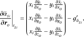 (B.15)
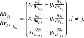 (B.16)
Similarly, the position partials of  are written as follows:
 (B.17)
 (B.18)
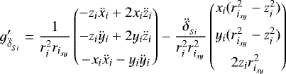
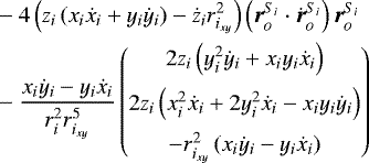
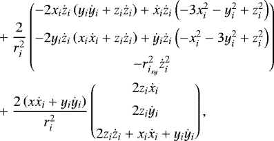 (B.19)
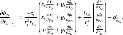 (B.20)
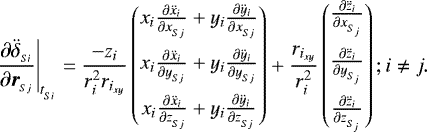 (B.21)
Finally, the velocity partials also have to be derived for  and
and  . We again split the partials expressions into two terms, designated by
  and
and  (or
(or  and
and  ). Again
  corresponds to the contribution of the acceleration partials. Starting with the partials of
  with respect to the satellites’ and observer’s velocity vectors, we obtain the following expressions:

Lastly, we obtain the following formulations for the partials of  with respect to the satellites’ and observer’s velocity vectors:
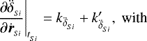 (B.27)
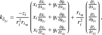 (B.28)
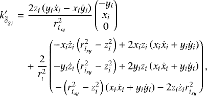 (B.29)
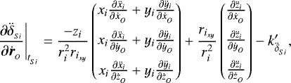 (B.30)
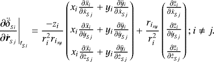 (B.31)
Appendix C Acceleration partials
As shown in Appendix B, computing  and
and  partials requires to first compute the partials of those relative acceleration, starting from Eq. (4):
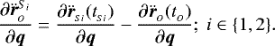 (C.1)
(C.1)
The vector of parameters q can either refer to one of the satellites state  or to the observer state
  . We first consider the partials with respect to the observer state, given by
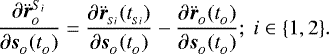 (C.2)
(C.2)
The acceleration  of the satellite i at time
  depends on the observer state
  at
at  , assuming the observer’s body indeed exerts an acceleration on satellite i (although such acceleration is usually negligible, see simplifying assumptions discussed at the end of this appendix). Equation (C.2) must thus be rewritten as
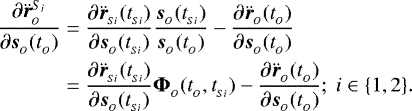 (C.3)
(C.3)
Similarly, acceleration partials with respect to the two satellites’ states are expressed as follows:

According to Eqs. (C.3)–(C.5), four state transition matrices need to be computed. However, a few remarks must be considered, in light of the computational effort this would require. For mutual approximations between the Galilean moons observed from the Earth, the satellite-observer distance is comparable between the two satellites. The difference between the two times  and
and  is thus very small, and the state transition matrices
  (with {i, j}∈{1, 2} and j≠i) are consequently close to unit matrices.
The difference between each time  and the observation time
  is larger. However, looking at Eqs. (C.3)–(C.5), the state transition matrices
  and
and  are always multiplied by partials of the observer’s body acceleration with respect to one of the satellite’s state, or the other way around. Considering the large satellites–observer distances, these accelerations partials can actually be neglected.
Overall, for mutual approximations between Galilean moons, the state transition matrices appearing in Eqs. (C.3)–(C.5) can be either approximated by unit matrices, or the entire acceleration partial term they contribute to can be neglected. This significantly simplifies the implementation and reduces the computational effort. Acceleration partials are anyway only required to compute the partials of  and
and  , which represent a marginal contribution of the total central instant partials (see Sect. 2.4). Simplifying assumptions to compute those acceleration partials can therefore be made safely.
Appendix D Verification of the analytical partials
Comparison between analytical and numerical solutions for the changes in central instants.
The central instants partials derived in Sect. 2.3 were validated numerically, by comparing the analytically estimated change in central instant with the actual change obtained when applying a small variation to the estimated parameters. Partials were expressed with respect to  ,
,  and
and  (for the first satellite’s, second satellite’s and observer’s states, respectively). Analytical approximations of the changes in central instants were derived from the observation partials with respect to the initial state of interest, multiplied with the appropriate state transition matrix, as follows:

The results of the numerical verification are reported in Table D.1. The extremely low differences found between the analytical and numerical changes in central instant prove the validity of our analytical partials.
Appendix E Contribution of the  and
and  partials to the central instant partials
Table E.1 gives the relative contributions of the  and
and  partials to the total central instant partials. They are reported for the first five Io-Europa mutual approximations in 2020 and are shown to be negligible.
Appendix F Alternative observables’ weights for past mutual approximations (2016–2018 observational campaign)
We computed the alternative observables’ weights for the past mutual approximations observed during the 2016–2018 campaign, which are provided in Morgado et al. (2019). Tables F.1–F.3 contain the weight values obtained with Eq. (41), following the weighting strategy described in Sect. 3.3 (we have shown this approach to be crucial to obtain consistent estimation solutions between central instants and alternative observable in Sect. 4.4).
For consistency purposes, the errors in central instant σ(tc) given in Morgado et al. (2019) were translated into errors in the alternative observable σalt. using the same ephemerides as the ones used in Morgado et al. (2019; i.e. JUP310 with DE435 from JPL). Table F.1 corresponds to mutual approximations observed in 2016, while Tables F.2 and F.3 are dedicated to 2017 and 2018 observations, respectively. The geodetic coordinates of the six different ground stations can be found in Morgado et al. (2019). We recommend to use the computed weight values σalt. when including the 2016–2018 observations in the state estimation with alternative observables.
Relative contributions of the  and
and  partials to the total central instants partials.
Appropriate weights for alternative observables, for the mutual approximations observed in 2016.
Appropriate weights for alternative observables, for the mutual approximations observed in 2017.
Appropriate weights for alternative observables, for the mutual approximations observed in 2018.
References
- Arlot, J.-E., Bernard, A., Merlin, P., et al. 1982, A&A, 111, 151 [Google Scholar]
- Arlot, J.-E., Emelyanov, N., Varfolomeev, M., et al. 2014, A&A, 572, A120 [NASA ADS] [CrossRef] [EDP Sciences] [Google Scholar]
- Crida, A., & Charnoz, S. 2012, Science, 338, 1196 [Google Scholar]
- Ćuk, M., Dones, L., & Nesvornỳ, D. 2016, ApJ, 820, 97 [Google Scholar]
- Dias-Oliveira, A., Vieira-Martins, R., Assafin, M., et al. 2013, MNRAS, 432, 225 [Google Scholar]
- Dirkx, D., Lainey, V., Gurvits, L., & Visser, P. 2016, Planet. Space Sci., 134, 82 [Google Scholar]
- Dirkx, D., Mooij, E., & Root, B. 2019, Astrophys. Space Sci., 364, 37 [Google Scholar]
- Emelyanov, N. 2009, MNRAS, 394, 1037 [Google Scholar]
- Emelyanov, N. 2017, MNRAS, 469, 4889 [Google Scholar]
- Emelyanov, N., Andreev, M., Berezhnoi, A., et al. 2011, Solar Syst. Res., 45, 264 [Google Scholar]
- Fuller, J., Luan, J., & Quataert, E. 2016, MNRAS, 458, 3867 [NASA ADS] [CrossRef] [Google Scholar]
- Heller, R., Marleau, G.-D., & Pudritz, R. E. 2015, A&A, 579, L4 [NASA ADS] [CrossRef] [EDP Sciences] [Google Scholar]
- Kiseleva, T., Izmailov, I., Kiselev, A., Khrutskaya, E., & Khovritchev, M. Y. 2008, Planet. Space Sci., 56, 1908 [Google Scholar]
- Lainey, V., Arlot, J.-E., Karatekin, Ö., & Van Hoolst T. 2009, Nature, 459, 957 [Google Scholar]
- Lainey, V., Duriez, L., & Vienne, A. 2004, A&A, 420, 1171 [NASA ADS] [CrossRef] [EDP Sciences] [Google Scholar]
- Lainey, V., Karatekin, Ö., Desmars, J., et al. 2012, ApJ, 752, 14 [Google Scholar]
- Lainey, V., Casajus, L. G., Fuller, J., et al. 2020, Nat. Astron., 1 [Google Scholar]
- Lunine, J. I. 2017, Acta Astron., 131, 123 [Google Scholar]
- Lynam, A. E., & Longuski, J. M. 2012, Acta Astron., 79, 33 [Google Scholar]
- Marion, G. M., Fritsen, C. H., Eicken, H., & Payne, M. C. 2003, Astrobiology, 3, 785 [Google Scholar]
- Morgado, B., Assafin, M., Vieira-Martins, R., et al. 2016, MNRAS, 460, 4086 [Google Scholar]
- Morgado, B., Vieira-Martins, R., Assafin, M., et al. 2019, MNRAS, 482, 5190 [Google Scholar]
- Moyer, T. D. 2000, Formulation for Observed and Computed Values of Deep Space Network Data Types for Navigation, 3 (John Wiley & Sons) [Google Scholar]
- Murrow, D., & Jacobson, R. 1988, in Astrodynamics Conference, 4249 [Google Scholar]
- Parkinson, C. D., Liang, M.-C., Yung, Y. L., & Kirschivnk, J. L. 2008, Origins Life Evol. Biospheres, 38, 355 [Google Scholar]
- Pascu, D., Morrison, L., & Gilmore, G. 1994, Galactic and Solar System Optical Astrometry (Cambridge University Press) [Google Scholar]
- Peng, Q. Y., Vienne, A., Wu, X., Gan, L., & Desmars, J. 2008, ApJ, 136, 2214 [Google Scholar]
- Peng, Q., He, H., Lainey, V., & Vienne, A. 2012, MNRAS, 419, 1977 [Google Scholar]
- Raofi, B., Guman, M., & Potts, C. 2000, in Astrodynamics Specialist Conference, 4035 [Google Scholar]
- Robert, V., Saquet, E., Colas, F., & Arlot, J.-E. 2017, MNRAS, 467, 694 [Google Scholar]
- Samuel, H., Lognonné, P., Panning, M., & Lainey, V. 2019, Nature, 569, 523 [Google Scholar]
- Stone, R. C. 2001, ApJ, 122, 2723 [Google Scholar]
- Weisstein, E. W. 2002, https://mathworld.wolfram.com/ [Google Scholar]
All Tables
Improvements in the final errors obtained with central instants, using two different observations sets.
Comparison of the final formal errors obtained with the two types of observables, when applying constant weight values.
Comparison of the formal errors in the initial positions of the four Galilean moons.
Maximum absolute values for the residuals between the apparent distance history and the fitted polynomial.
Comparison between analytical and numerical solutions for the changes in central instants.
Relative contributions of the and partials to the total central instants partials.
Appropriate weights for alternative observables, for the mutual approximations observed in 2016.
Appropriate weights for alternative observables, for the mutual approximations observed in 2017.
Appropriate weights for alternative observables, for the mutual approximations observed in 2018.
All Figures
|
Fig. 1 Observation of a mutual approximation (i.e. close encounter between two natural satellites). The apparent distance between the two satellites (blue dots in the top panel) is frequently measured and a polynomial is used to fit these observationsand estimate the central instant of the close encounter (typically fourth-order polynomial, displayed in red). The residuals between the apparent distances measurements and the fitted polynomial are shown in black (bottom panel). |
| In the text | |
|
Fig. 2 Schematic representation of the different coordinate systems and positions. The first satellite and all associated notations are depicted in red, while blue is used for the second satellite.
|
| In the text | |
|
Fig. 3 Distribution of the simulated mutual approximations per year, depending on the ground station (panel a) and on the two moons involved (panel b). Mutual approximations which have been discarded to mimic the effect of bad weather conditions are not included in this distribution. |
| In the text | |
|
Fig. 4 Time evolution of the formal errors in Io’s and Europa’s initial RSW coordinates (radial, normal, and axial directions, see Fig. 2), as more observations are progressively included in the state estimation. The blue line displays the time evolution of the formal errors obtained by using the central instants as observables (left y-axis). The red line corresponds to the time evolution of the formal errors obtained from alternative observables (left y-axis too). The initial values of the formal errors, before including any observation, correspond to the a priori covariance values used for the regularisation (i.e. 100 km, see Sect. 3.2). The grey line (right y-axis) represents the relative difference (in percentage) between the two solutions as a function of time. The formal errors are equal to their initial values until the inclusion of the first mutual approximation (towards the end of 2021) and no difference between the two observables’ solutions is thus observed beforehand. |
| In the text | |
|
Fig. 5 Reduction in formal errors obtained by using central instants instead of alternative observables, as more observations are added to the solution. It is displayed on the left axis, for the three position components in RSW frame (panel a: Io, panel b: Europa). On the right axis (purple dots), the ratio between the normalised contributions of central instants over their corresponding alternative observables is displayed, for each mutual approximation (normalised contributions are computed as in Eq. (43)). As mentioned in Sect. 3.1, the first simulated observation only occurs towards the end of 2021, hence the lack of data beforehand. |
| In the text | |
|
Fig. 6 Observations’ contributions to the estimated initial positions’ solution (in colours), as a function of each mutual approximation’s characteristics (impact parameters and impact velocities, reported on the x- and y-axes, respectively). Panel a: normalised contribution of each mutual approximation to the solution (averaged between Io and Europa), when using central instants. Panel b: ratio between the normalised contributions of central instants over their corresponding alternative observables. The normalised contribution of each mutual approximation to the solution is obtained with Eq. (43). |
| In the text | |
|
Fig. 7 Effect of the inertial geometry on the mutual approximations’ impact characteristics. Both the impact parameter and the inertial distance between Io and Europa (as opposed to apparent distance as seen from the ground stations) are displayed, for each mutual approximation. The colours represent the time at which the observation is made. |
| In the text | |
|
Fig. 8 Effect of the observation geometry on the mutual approximations’ impact parameters. The angle between the orbital plane of the Galilean moons and the observation vectors (Earth-Io in black and Earth-Europa in red) is plotted for each mutual approximation. The corresponding impact parameters (in as) are represented by blue dots. |
| In the text | |
|
Fig. 9 Propagated formal errors in position components over the observational period (panel a: Io, panel b: Europa). The errors in position are expressed in the RSW frame (see Fig. 2) and are obtained from the propagated covariance matrix and estimated initial states. The purple dots (right axis) display the ratio between the normalised contributions of central instants over their corresponding alternative observables, for each mutual approximation. |
| In the text | |
|
Fig. 10 Normalised contribution of mutual approximations between Io and Europa (I-E, left plots), Io and Ganymede (I-G, centre-left plots), Io and Callisto (I-C, centre-right plots), Europa and Ganymede (E-G, right plots) to the initial position of Io (blue), Europa (orange), Ganymede (green), and Callisto (purple). Results for Europa-Callisto and Ganymede-Callisto mutual approximations are not represented here, but do not show any trend that is not already highlighted by the contributions of the other observations. The first simulated observation only happens at the end of year 2021, explaining the lack of data before that date. |
| In the text | |
|
Fig. A.1 Apparent distance measurements during a mutual approximation (blue dots on top panels). The polynomial used to fit these observations is typically a fourth order one (left panel). A second order polynomial was also tested, for the whole duration of the event (middle panels) and over a reduced time interval (30 min) centred on the central instant tc. For each of the three case, the residuals between the fitted polynomial and the true apparent distance history are displayed in the bottom panels. |
| In the text | |
Current usage metrics show cumulative count of Article Views (full-text article views including HTML views, PDF and ePub downloads, according to the available data) and Abstracts Views on Vision4Press platform.
Data correspond to usage on the plateform after 2015. The current usage metrics is available 48-96 hours after online publication and is updated daily on week days.
Initial download of the metrics may take a while.