| Issue |
A&A
Volume 644, December 2020
|
|
|---|---|---|
| Article Number | A95 | |
| Number of page(s) | 16 | |
| Section | Galactic structure, stellar clusters and populations | |
| DOI | https://doi.org/10.1051/0004-6361/202039145 | |
| Published online | 04 December 2020 | |
Separation between RR Lyrae and type II Cepheids and their importance for a distance determination: the case of omega Cen⋆
1
INAF-Osservatorio Astronomico di Roma, Via Frascati 33, 00040 Monte Porzio Catone, Italy
e-mail: vittorio.braga@inaf.it
2
Space Science Data Center, Via del Politecnico snc, 00133 Roma, Italy
3
Dipartimento di Fisica, Università di Roma Tor Vergata, Via della Ricerca Scientifica 1, 00133 Roma, Italy
4
Herzberg Astronomy and Astrophysics, National Research Council, 5071 West Saanich Road, Victoria, British Columbia V9E 2E7, Canada
5
INAF-Osservatorio Astronomico di Capodimonte, Salita Moiariello 16, 80131 Napoli, Italy
6
Astrophysics Research Institute, Liverpool John Moores University, IC2, Liverpool Science Park, 146 Brownlow Hill, Liverpool L3 5RF, UK
7
Department of Astronomy, University of Michigan, Ann Arbor, MI, USA
8
Department of Astronomy, The University of Tokyo, 7-3-1 Hongo, Bunkyo-ku, Tokyo 113-0033, Japan
9
Instituto de Astrofísica de Canarias, Calle Via Lactea s/n, 38205 La Laguna, Tenerife, Spain
10
Department of Astronomy, University of Washington, Seattle, WA 98195, USA
Received:
10
August
2020
Accepted:
12
October
2020
The separation between RR Lyrae (RRLs) and type II Cepheid (T2Cs) variables based on their period is debated. Both types of variable stars are distance indicators, and we aim to promote the use of T2Cs as distance indicators in synergy with RRLs. We adopted new and existing optical and near-infrared (NIR) photometry of ω Cen to investigate several diagnostics (color-magnitude diagram, Bailey diagram, Fourier decomposition of the light curve, and amplitude ratios) for their empirical separation. We found that the classical period threshold at one day is not universal and does not dictate the evolutionary stage: V92 has a period of 1.3 days but is likely to be still in its core helium-burning phase, which is typical of RRLs. We also derived NIR period-luminosity relations and found a distance modulus of 13.65 ± 0.07 (err.) ± 0.01 (σ) mag, in agreement with the recent literature. We also found that RRLs and T2Cs obey the same period-luminosity relations in the NIR. This equivalence provides the opportunity of adopting RRLs+T2Cs as an alternative to classical Cepheids to calibrate the extragalactic distance scale.
Key words: stars: variables: Cepheids / stars: variables: RR Lyrae / galaxies: clusters: individual: ω Cen / stars: distances
Full Table 3 is only available at the CDS via anonymous ftp to cdsarc.u-strasbg.fr (130.79.128.5) or via http://cdsarc.u-strasbg.fr/viz-bin/cat/J/A+A/644/A95
© ESO 2020
1. Introduction
Type II Cepheids (T2Cs) are pulsating variable stars of the Cepheid instability strip (IS). They are typically associated with old (> 10 Gyr) stellar populations. They are low-mass stars in either the post-horizontal branch (post-HB), asymptotic giant branch (AGB), or post-AGB phase (see, e.g., Gingold 1974; Sweigart et al. 1989; Bono et al. 1997a, 2020) and are mostly found in stellar systems with extended blue HBs (BHB). T2Cs can be used as standard candles for distance estimates because they display optical and near-infrared (NIR) period-luminosity (PL) relations, analogous to those of RR Lyrae (RRLs) and classical Cepheids (CCs). Moreover, the PL relations of T2Cs are only minimally affected by metal abundance (Bono et al. 1997a; Matsunaga et al. 2006, 2013; Di Criscienzo et al. 2007; Lemasle et al. 2015).
Although they are far less numerous than RRLs (the Galactic bulge hosts almost 70 000 RRLs, but only about 1000 T2Cs; Soszyński et al. 2014, 2017, 2019), T2Cs are brighter by one to five mag. This means that detecting them in high-extinction environments (e.g., the Galactic bulge, Bhardwaj et al. 2017a; Braga et al. 2018a, 2019) is easier, but also that they can be identified and characterized in external galaxies. T2Cs have been found near M 31 (Kodric et al. 2018) in M 101 and M 106 (Stetson et al. 1998; Macri et al. 2006; Majaess et al. 2009), and more recently, even an RV Tauri (RVT) has been reoported in the Seyfert 1 galaxy NGC 4151 (Yuan et al. 2020).
In particular, T2Cs seem to follow the same PL relations as RRLs (Majaess 2010) in the NIR bands (JHKs), although solid empirical evidence is still lacking. This means that RRLs and T2Cs might be adopted jointly to calibrate supernova type Ia (SNIa) luminosities, and in turn, to measure the Hubble constant (H0). In the past years, a discrepancy of ∼4σ between estimates of the local value H0 from the CCs+SNIa scale (H0 = 74.03 ± 1.42 km s−1 Mpc−1; Riess et al. 2019) and from Cosmic Microwave Background analyses (H0 = 67.39 ± 0.54 km s−1 Mpc−1; Planck Collaboration VI 2020) has arisen, meaning that either a bias in any of these techniques or new physics come into play. The discussion about the extent of the current discrepancy is far from being settled. In a recent investigation, Majaess (2020) argued that neglected or inaccurate blending corrections may result in an overestimated H0. Moreover, when a new calibration of SNIa based on the luminosity of the tip of the red giant branch (TRGB, Beaton et al. 2019) is used, the discrepancy caused by the intermediate values of H0 (69.6 ± 1.7 km s−1 Mpc−1Freedman et al. 2020) appears to be alleviated.
An independent estimate of the local H0 obtained with RRLs+T2Cs might be crucial to either validate or reconsider the discrepancy. When RRLs+T2Cs were adopted instead of CCs, a population bias would also be removed because the latter variables are only found in late-type galaxies, while RRLs and T2Cs are ubiquitous. A calibration of SNIa distances through old-population tracers, RRLs and TRGB, has been proposed before (Beaton et al. 2016), but this approach requires one more intermediate calibrations (that from RRLs to the TRGB), brings into play different physics (TRGB stars are not pulsating variables), and in turn, different systematics when compared with homogeneous PL relations for RRLs and T2Cs.
The separation between RRLs and T2Cs is a long-standing problem. As a first approximation, it is possible to adopt a period threshold, whose exact value is still a matter of debate. A threshold of ∼0.8 days was set in the review by Gautschy & Saio (1996) where type 1 (AHB1) stars above the HB, as defined in Strom et al. (1970) and Diethelm (1983, 1990), were considered as T2Cs rather than evolved RRLs. This threshold is obsolete, however, because a more extended and homogeneous investigation, based on period distribution and on the Fourier parameters of the light curve of RRLs in the Galactic bulge, has now set the threshold at one day (Soszyński et al. 2008, 2014).
The RRLs in the bulge have a primordial (or minimally enhanced) helium abundance (Marconi & Minniti 2018), but there is theoretical evidence that helium enhancement increases the periods of RRLs (Marconi et al. 2018). This means that a one-day period threshold should be considered a particular case of a more generic chemical-, physics-, and evolution-dependent threshold.
The T2Cs are typically separated into BL Herculis (BLHs), W Virginis (WVs), and RV Tauri (RVTs) stars. The investigation by Soszyński et al. (2011) of the Optical Gravitattional Lensing Experiment (OGLE)-III data found two minima at 5 and 20 days in the period distribution of 335 T2Cs in the Galactic bulge. They adopted these values as thresholds between BLHs-WVs and WVs-RVTs, respectively. These thresholds were later validated on the OGLE-IV sample of bulge T2Cs, which is almost three times larger (Soszyński et al. 2017). The BLHs-WVs threshold of the General Catalog of Variable Stars (GCVS, Samus’ et al. 2017) is 4 days, based on the period distribution of T2Cs in the Large Magellanic Cloud (LMC; Soszyński et al. 2008). However, this is based on a small sample (∼200 T2Cs), and new LMC data (> 300 T2Cs, Soszyński et al. 2018) invalidate the 4 day threshold.
Whether RVTs should be all classified as bona fide T2Cs is still a pending issue. RVTs are associated with either low- or intermediate-mass (from ∼0.5 up to ∼3 M⊙Dawson 1979) post-AGB stars (Gingold 1985; Wallerstein 2002), belonging to old- and intermediate-age populations, respectively. To further stress the importance of the difference between old- and intermediate-age RVTs, a different naming was proposed for the low-mass RVTs (Catelan & Smith 2015, V2342 Sgr stars). There is empirical evidence that RVTs in Galactic globular clusters (GGCs), which should belong to the V2342 Sgr class, do not share the same properties as field RVTs (Zsoldos 1998, e.g., they are missing the typical alternating deep and shallow minima). Finally, there is no consensus about the use of RVTs as reliable distance indicators. It is still a matter of debate whether they follow the PL relation of BLHs and WVs (Matsunaga et al. 2006; Ripepi et al. 2015; Bhardwaj et al. 2017b).
Among nearby coeval stellar systems, the GGC ω Cen (NGC 5139) is the best benchmark system for T2Cs. It hosts the largest T2C sample in GGCs (7 T2Cs) after the two more metal-rich clusters NGC 6388 (12) and NGC 6441 (8), as well as long-period (> 0.7 days) RRLs. Moreover, 3 of its T2Cs have periods shorter than two days, which is optimal for investigating the transition between RRLs and T2Cs, while the periods of all T2Cs in NGC 6388 and NGC 6441 are longer than two days, with only one exception. While it is true that the bulge hosts more RRLs and T2Cs, they are not at the same distance, the differential reddening and the stellar crowding are more severe, and NIR time series are only available for the Ks band.
Furthermore, ω Cen is characterized by a well-known spread in metallicity (Johnson & Pilachowski 2010; Johnson et al. 2020) and in helium content (Lee et al. 1999; Calamida et al. 2020) and has a peculiar radial distribution of metal-poor and metal-rich stellar populations (Lee et al. 1999; Calamida et al. 2020, and references therein). This is an advantage because the pulsation properties of RRLs and T2Cs depend on chemical composition, meaning that in the CGC ω Cen these variable stars have more heterogeneous and varied pulsation properties.
Recently, the unprecedented wealth of kinematic data from Gaia DR2 and APOGEE DR14 (Gaia Collaboration 2018; Abolfathi et al. 2018) were employed by Ibata et al. (2019) to validate the existence of the tidal stellar stream of ω Cen. Based on its motion, Myeong et al. (2019) argued that ω Cen could have been accreted by the Milky Way during the Sequoia merger, while Massari et al. (2019) and Kruijssen et al. (2020) more conservatively associated ω Cen with either Sequoia or the larger Gaia-Enceladus (Helmi et al. 2018) merger event. On the theoretical side, Bekki & Tsujimoto (2019) validated these hypotheses and speculated that ω Cen was a GGC of an accreted galaxy. Based on the properties of the different stellar population of ω Cen, Calamida et al. (2020) proposed that before it was accreted by the Milky Way, ω Cen might have formed by mergers between clusters and eventually a merger with the nucleus of a dwarf galaxy.
Therefore ω Cen is not only a GGC with optimal properties for investigating T2Cs, but also a very interesting object on its own. It is the largest and most heterogeneous GGC within the Galaxy. Finally, because it close and well populated, its distance was estimated using several diagnostics (RRLs, T2Cs, TRGB, white dwarfs, and eclipsing binaries).
The aim of the paper is to provide more rigorous criteria to distinguish between RRLs and T2C by viewing them from an evolutionary perspective. This would be a complete reversal of the point of view. The period threshold has so far been the most common criterion for separating RRLs and T2Cs. This separation almost always separates HB stars on the one hand (P < one day) and post-HB stars on the other hand (P > one day). As a consequence, RRLs are considered as HB (core He burning) stars and T2Cs are considered as post-HB (double shell burning) stars. Our claim instead is that the leading argument for separating RRLs and T2Cs is their evolutionary stage, and that the empirical separation, which is only based on pulsation properties, is the consequence.
Moreover, we plan to adopt T2Cs as distance indicators, compare them with RRLs, and use them jointly within a common distance diagnostic. This means that on the one hand, we aim for a more solid understanding of the differences in the evolutionary properties of both RRLs and T2Cs, and on the other hand, we use them together as a single distance indicator. The two aims appear to be at odds, but this is not the case. For distance determinations (especially of Local Group galaxies), it would be a threefold advantage to adopt a common PL relation because (i) RRLs complement the small number of T2Cs; (ii) T2Cs complement the lower brightness of RRLs, and (iii) together, they provide a wider period range on which to calibrate the relation, as has been suggested by Benedict et al. (2011). Still, RRLs and T2Cs are not the same objects from the evolutionary point of view, and it is important to provide a clear criterion for telling them apart not only for a mere taxonomical purpose, but also for the correct development of pulsation models (Bono et al. 2020) and for investigating the population ratios of the host stellar system (GCs, nearby galaxies, etc.).
The paper is structured as follows: in Sect. 2 we discuss the pulsation properties of T2Cs and long-period RRLs in ω Cen; moreover, we discuss the transition between the two types of variables, also based on bulge T2Cs. Section 3 is devoted to the comparison of the Bailey diagram and amplitude ratios of the T2Cs in ω Cen with those in the Galactic halo and bulge. We discuss the PL relations of T2Cs, their comparison with the PLs of RRLs, and use them to estimate the distance of ω Cen in Sect. 4. We discuss our results in Sect. 5.
2. Type II Cepheids
According to the catalog of variable stars in GGCs by Clement et al. (2001), ω Cen is the third richest GGC in T2Cs, after the metal-rich clusters NGC 6388 and NGC 6441. ω Cen hosts seven T2Cs: five BLHs (V43, V48, V60, V61, and V92), one WV (V29), and one RVT (V1). All these variables have been discovered in the first investigation of variable stars in ω Cen (Bailey 1902). A detailed list of the T2Cs and their pulsation properties is provided in Appendices A and B.
2.1. Transition between RRLs and T2Cs
The period threshold between RRLs and T2Cs is a long-standing dilemma in the field of pulsating variables. In the literature, the accepted values for the maximum period of RRLs range from 0.75 days (Wallerstein & Cox 1984) to 2.5 days (Diethelm 1983).
An investigation of a homogeneous and extended sample of RRLs and T2Cs in the LMC with VI-band OGLE photometry allowed establishing a more solid empirical threshold at one day (Soszyński et al. 2008). This was based on the period distribution and on the position of the pulsating variables in the log P − ϕ21 plane, where ϕ21 is one of the coefficients of the Fourier -series fit to the light curve.
As stated in the Introduction, the threshold at one day should be considered as a lower limit in the case of a cosmological helium abundance. RRL pulsation models (Marconi et al. 2018) predict longer pulsation periods for RRLs with a helium-enhanced chemical composition. In stellar systems hosting helium-enhanced stellar populations, the one-day threshold might therefore not be reliable, and the separation between RRLs and BLHs might be less sharp. Recently, Kovtyukh et al. (2018a) hypothesized that the very existence of BLHs is to be ascribed to helium enhancement in a progenitor mass of 0.8 M⊙. This is consistent with the fact that the BHB of the metal-rich GGCs NGC 6441 and NGC 6388 (the two GGCs hosting the highest number of T2Cs) can be reproduced by helium-enhanced (Y = 0.35 − 0.40) HB models (Busso et al. 2007; Bellini et al. 2013). Dalessandro et al. (2011) and Tailo et al. (2019) showed that the initial helium content also affects the mass loss on the Red Giant Branch (RGB) and in turn the position of the stars on the HB. The more helium-enhanced the progenitor, the less massive and bluer the star on the Zero-Age HB (ZAHB), both because the mass loss is higher and because at fixed age and fixed mass-loss rate, the turn-off mass is lower. Helium enhancement would therefore favor an evolution to T2Cs, which are observed only in systems with a well-populated BHB. However, there is no evidence of an extensive helium-enhanced population in the halo, thick-disk, and old population of the Galactic bulge, where Galactic T2Cs are found. This means that while helium enhancement might favor the formation of T2Cs, it is not the only requirement. Moreover, evolved helium-enhanced RRLs might have periods and luminosities similar to those of BLHs (Marconi et al. 2018).
For this purpose, ω Cen is the most appropriate stellar system in which to inspect the RRL-BLH separation for several reasons: (i) ω Cen displays a well-defined BHB (Castellani et al. 2007), and T2Cs are associated with stellar systems showing an extended HB because their progenitors are mainly BHB stars (Beaton et al. 2018; Bono et al. 2020). (ii) It hosts five RRLs with periods between 0.85 and one day (Navarrete et al. 2015; Braga et al. 2016) and four BLHs with a period shorter than three days (V43, V60, V61 and V92); (iii) There is evidence that the HB of ω Cen should at least in part be enhanced in helium content (Cassisi et al. 2009; Bellini et al. 2013; Tailo et al. 2016; Latour et al. 2018, Y ∼ 0.28−0.38).
We investigated the transition between RRLs and T2Cs using the Color-Magnitude Diagram (CMD), Bailey diagram, and the Fourier parameters of the light-curve fit. The latter two diagnostics were not used for the long-period RRLs because our sampling of the time series is not optimal for variables with periods too close to one day (V263 and NV366), and we have too few I-band phase points for the other variables.
The rate of the period change is not one of the quoted diagnostics because the sampling of our data does not allow us to provide accurate measures of this parameter. Recent theoretical results about the evolutionary channels producing T2Cs (Bono et al. 2020) show that a significant fraction of T2Cs evolve from the blue to the red side of the Hertzsprung-Russel Diagram (HRD). These are low-mass (0.495 ≤ M/M⊙ < 0.55) HB stars that evolve toward the AGB after the central helium is exhausted. In subsequent evolutionary phases, they move back to the blue toward the White Dwarf (WD) sequence, but this occurs at higher luminosities (WVs and RVTs). These objects are characterized in their fainter limit by positive period derivatives. However, these models might also perform several gravo-nuclear loops (Bono et al. 1997b,c; Constantino et al. 2016) in the HRD either during the AGB phase and/or in their approach to the WD cooling sequence. Some of these loops take place inside the IS, and the period derivative can in turn attain both positive and negative values.
Evolutionary models also show that long-period RRLs evolve from the blue to the red (see Fig. 5 in Bono et al. 2020). This means that positive-period derivatives do not help in distinguishing between long-period RRLs and short-period T2Cs. On the other hand, both positive and negative period derivatives can be univocally associated with T2Cs. The current empirical evidence indicates that period derivatives for the short-period BLHs of ω Cen are positive (Jurcsik et al. 2001). Therefore they cannot help us in separating BLHs from RRLs.
2.2. Long-period RRLs
We inspected five RRLs with P > 0.85 days (V91, V104, V150, V263, and NV366). We did not include NV455 because we do not have data for this star, which is located more than 40 arcmin from the center. There is a clear period gap at ∼0.935−0.995 days in which no RRLs are found. Unfortunately, there are no strong arguments to assess whether the gap is real or just due to the poor statistics of long-period RRLs.
V91, V104, and V150. These variables are all below the period gap, and their position in the V, B − I and K, B − K CMDs (see Fig. B.3) is consistent with being bona fide RRLs. In the Bailey diagram, they are in the locus derived by performing a linear fit of Amp(V) versus period of the RRab stars of NGC 6388 and NGC 6441 (Amp(V) = 2.30 − 2.04 ⋅ P, see Fig. B.4). These clusters have been defined as Oosterhoff III in the literature, but we decided to call them Oosterhoff 0 (Oo0, Braga et al. 2016) because these GGCs are very metal rich ([Fe/H] < 1 dex) and the progression in metallicity is replicated by the numbers (Oo0 = metal-rich; OoI = metal-poor; OoII = very metal-poor).
V263. This star is above the period gap (P = ∼1.01 days), but its pulsation amplitude is very small and appears to agree well with the decreasing trend of RRab amplitudes at long periods (see Fig. B.4). Despite its very long period, this star is consistent with being an RRab because of its position in the CMDs, which is well within the magnitude range of HB stars with the same color.
NV366. The light curve is heavily aliased because its period is 0.9999 days (above the period gap). The phases around minimum are missing in the optical bands. In the NIR bands, only the upper part of the decreasing branch is sampled. Therefore both the optical and the NIR mean magnitudes that we derived are probably underestimated, and the amplitudes are not reliable. However, in both CMDs, it is placed within the HB. Although it is located ∼3.05 arcmin from the cluster center in a very crowded region, a visual inspection of the images did not outline any sign of blending. However, the crowding probably affects the photometric calibration between our different optical datasets (Braga et al. 2016).
We note from the Bailey diagrams in Fig. B.4 that a sizeable sample of ω Cen RRLs, including the five discussed above, is placed in the locus of RRab stars in Oo0 clusters. The debate regarding the relation between the high metallicity of Oo0 clusters and the properties of their HB and RRLs is still ongoing. Pritzl et al. (2002) invoked a bimodal distribution of metallicities in the Oo0 clusters in which RRLs and BHB stars belong to the more metal-poor population. In this scenario, HB stars evolve to the red, thus crossing the IS as metal-poor off-ZAHB RRLs. However, low-resolution spectra of RRLs in NGC 6441 provide high metallicities for these stars (Clementini et al. 2005), thus invalidating the scenario by Pritzl et al. (2002).
A similar scenario was described by Tailo et al. (2016) for ω Cen: Based on population synthesis, they found that RRLs in ω Cen should mostly be metal poor and evolved (off-ZAHB), with a smaller fraction of metal-rich and fainter ZAHB RRLs. Neither of these populations is significantly enhanced in helium (Y ≤ 0.28).
We compared the empirical distribution of the RRLs and of the BHB in ω Cen with the BaSTI α-enhanced, helium-standard, Z = 0.0006 and Z = 0.004 tracks (corresponding to [Fe/H] ∼ −1.84 and [Fe/H] ∼ −1.01, respectively, see Fig. 1). The two metallicity values were chosen to reproduce the peak of the metallicity distribution of RRLs (Magurno et al. 2019) and its metal-rich extension, which is the most prominent tail of the distribution. The majority of RRLs overlaps the most metal-poor ZAHB model. On the other hand, the metal-rich ZAHB better fits the fainter and presumably more metal-rich RRLs.
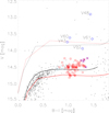 |
Fig. 1. Optical (V vs. B − I) CMD of ω Cen. Light blue circles show RRc, red squares present RRab, purple asterisks indicate long-period-RRab, and blue diamonds show BLHs. Black and red lines display the ZAHB (solid) and helium-exhaustion (dotted) sequences for α-enhanced, helium-normal HB models (Pietrinferni et al. 2006) for two different metal contents: Z = 0.0006 ([Fe/H] = −1.84) and Z = 0.004 ([Fe/H] = −1.01). |
We confirmed that none of the Oo0-like RRLs in ω Cen belongs to the faint part of the RRL sample. Based on the analysis of high-resolution spectra, Magurno et al. (2019) indeed found a minority of metal-poor RRLs. However, the latter are not significantly fainter in the V band than the metal-poor RRLs, therefore no firm conclusion can be reached.
This means that while it is reasonable to assume that evolution is the most important factor in generating Oo0-like RRLs, secondary factors also need to be considered to reproduce the observations in detail. Moreover, their metallicity is not necessarily low.
One factor might be the initial helium abundance. Marconi et al. (2011) investigated the period distribution of the RRLs in ω Cen and its correlation with helium enhancement. They concluded that the latter might be a concurrent reason for the long periods of RRLs in ω Cen, but also placed an upper limit (20%) on the fraction of helium-enhanced (Y ≥ 0.30) RRLs.
Another factor might be the mass on ZAHB: because mass-loss along the RGB evolution is likely at least partially a stochastic process, its correlation with Y or Z is not one-to-one. Stars with the same chemical abundance might therefore lose less or more than an average amount of mass on the RGB and will have cooler or higher temperatures on the ZAHB, as discussed by Origlia et al. (2007), van Loon (2008).
2.3. Short-period BLHs
The sources V43, V60, V61, and V92 are four BLHs with periods shorter than three days. We inspected their photometric properties to assess whether they might be better classified as very long-period RRLs, either evolved HB stars or helium enhanced. For this purpose, we adopted two different diagnostics: evolutionary and pulsation models, and Fourier coefficients.
Evolutionary and pulsation models: Fig. 1 shows that V92 is consistently fainter than the helium-exhaustion track. This is a further argument to reconsider its classification. We also point out that V43 is below the metal-rich helium-exhaustion track. However, we should assume a very high metallicity for V43 ([Fe/H] > 1.3 dex, which is typical of less than 10% of the RRL population of ω Cen, Magurno et al. 2019) to consider its reclassification as candidate RRab, while none of the other diagnostics points to a reclassification as a borderline RRab or BLH star.
Fourier coefficients: we derived the ϕ21 and ϕ31 Fourier coefficients of their V- and I-band light curves to compare them with those from the OGLE survey, which is the largest sample of Fourier coefficients of pulsating variable stars. OGLE provides only the I-band Fourier coefficients. Using OGLE V-band time series, we therefore derived the Fourier coefficients of the V-band light curves of bulge RRLs and T2Cs.
The top and middle panels of Fig. 2 display the V- (magenta) and I-band (blue) Fourier coefficients of OGLE bulge RRLs and T2Cs in the ϕ21 and ϕ31 versus log P diagrams. Larger symbols display the Fourier coefficients of the short-period BLHs in ω Cen. We did not derive the Fourier parameters of V61 and V92 in the I band because their light curve is not well sampled. However, we assume that their I-band coefficients are similar to or slightly higher than their V-band coefficients, as for all the other ω Cen and bulge variables in the two planes.
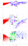 |
Fig. 2. Top: ϕ21 − log P diagram of long-period RRLs and short-period T2Cs in ω Cen and Galactic bulge. Red dots present RRab, blue dots show T2Cs (I-band Fourier coefficients), and magenta dots present T2Cs (V-band Fourier coefficients). Middle: same as the top panel, but for the ϕ31 coefficients. The green box contains variables in the short-period T2C sample, the black box contains variables in the candidate RRL sample, and the light blue box contains variables in the RRL template sample. Bottom: bailey diagram of the same variables as in the top and middle panel. Light blue, black, and green cicles display variables in the short-period T2C, candidate RRL, and RRL template samples, respectively. |
The sources V43, V48, and V61 are well within the typical loci of BLHs with the same period within the ϕ21 − log P and ϕ31 − log P diagrams. On the other hand, especially in the ϕ21 versus log P plane, V92 is at the edge of the bulge BLH locus. Moreover, its position is consistent with an extrapolation of the RRLs at longer periods. This provokes the question whether there might be RRLs with periods longer than one day within the sample of T2Cs in the bulge. To examine this hypothesis, we selected a few subsamples of bulge RRLs and T2Cs.
First, we selected 16 long-period (P > 0.97 d) RRLs (light blue box in the middle panel of Fig. 2) to build a light curve template of long-period RRLs (see Appendix D). Second, we selected two subgroups of T2Cs: One on the extension of the RRL locus in the ϕ31 − log P diagram (black box in the middle panel of Fig. 2), which we call “candidate RRLs” (15 objects, see Table 1), and the other at lower ϕ31 and longer periods (green box in the middle panel of Fig. 2), which we call “short-period T2Cs” (99 objects). The boxes have a purely empirical meaning and were only used to separate the two groups. The working hypothesis is that the stars in the first subgroup are indeed long-period RRLs.
Candidate RRab among bulge T2Cs.
To quantitatively validate this hypothesis, we fit the I-band light curves of both subgroups of variables with the RRL light-curve templates derived before. We found that the mean standard deviation from the fit of the light curves of the candidate RRLs is 0.016 ± 0.011 mag. For the second subgroup, the mean standard deviation is 0.045 ± 0.018 mag. Moreover, a visual inspection of the residuals of the light curves from the template fit (see Fig. 3) reveals that the light curves of the candidate RRLs are much closer to those of bona fide RRLs than the light curves of short-period T2Cs. While the residuals of the candidate RRLs from the template fit do not follow any trend with the phase, those of the short-period T2Cs show a clear periodic behavior, although this is not the same for all the stars. Finally, we found that the candidate RRLs are placed at the lower edge of the T2C distribution in the Bailey diagram (see the bottom panel of Fig. 2).
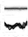 |
Fig. 3. Top: residuals of the I-band light curve of all candidate RRLs from the template fit. All the variables were phased with the period and epoch of maximum provided by OGLE, meaning that phase 0 is the phase of maximum brightness. Bottom: same as in the top panel, but for all the short-period T2Cs. |
Based on these considerations, we conservatively classify V92 as a candidate RRab variable. We point out that these classifications, although they are crucial for understanding the evolutionary status of the stars, are irrelevant concerning the period-luminosity relations and distance estimates because RRab and T2Cs do follow the same relations in the NIR (Matsunaga et al. 2006; Majaess 2010).
3. Comparison with type II Cepheids in other stellar systems
Type 2 Cepehids are not as numerous as RRLs, but they are found in all the regions of the Galaxy (bulge, halo, and GGCs), with the exception of the thin disk. They are also found in the Magellanic Clouds (MCs). Because their pulsation properties depend on the population (metallicity and age) properties of the host system, it is useful to adopt several diagnostics to compare the properties of T2Cs in ω Cen with those in other environments.
3.1. Bailey diagram: comparison with the halo
The Galactic halo is the most important component of the Galaxy in its merging history. The Gaia mission (Gaia Collaboration 2016) enabled the investigation in Galactic archaeology to reach its peak: streams and remnants from merged galaxies are being found, elucidating the past merging history of the Galaxy (Helmi et al. 2018; Myeong et al. 2019; Kruijssen et al. 2020; Helmi 2020). ω Cen itself most likely is a former GC of an accreted galaxy (either Gaia-Enceladus or Sequoia; Massari et al. 2019; Bekki & Tsujimoto 2019) that now orbits the Galactic halo.
It has been suggested that halo and GGC T2Cs belong to a different population by Woolley (1966). This was recently confirmed by Wallerstein & Farrell (2018) based on both kinematics and metal abundance. It is therefore interesting to compare the properties of ω Cen T2Cs with those in the halo. As a diagnostic, we adopt the Bailey diagram, which is independent of distance and reddening.
Figure 4 displays the optical (V-band) Bailey diagram of 362 halo T2Cs and ω Cen T2Cs. We adopted the catalog of Cepheids within Gaia DR2 published by Ripepi et al. (2019). However, we both complemented and corrected this list by comparing their classification with other surveys and literature data, namely, ASAS (Pojmanski 1997), ASASSN (Shappee et al. 2014; Jayasinghe et al. 2019), GCVS (Samus’ et al. 2017), and Warren & Harvey (1976). We provide in Table 2 the list of T2Cs that we added to the Ripepi et al. (2019) sample and those for which we have changed the classification.
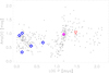 |
Fig. 4. Bailey diagram of T2Cs in the halo (gray points), and in ω Cen (same symbols as in Fig. 1, plus magenta star for the WV and an orange upside-down triangle for the RVT). |
Complements and changes to the Ripepi et al. (2019) T2C catalog.
We note that the halo field hosts T2Cs with periods longer than 100 days. This is a remarkable difference compared to T2Cs in all GGCs (V16 in NGC 6569 with a period of 87.5 days, Clement et al. 2001), and as we show in Sect. 3.2, with those in the Galactic bulge (the longest period is 84.8 days for T2Cs in the outer bulge, Soszyński et al. 2017 and 93.5 days for T2Cs in the inner bulge, Braga et al. 2019). This is further evidence that T2Cs in the halo belong to a different population than T2Cs in GGCs. We also note that the four short-period BLHs of ω Cen are placed at the edges of the distribution of field T2Cs. More precisely, V43 and V60 are at the high-amplitude edge, while V61 and V92 are placed at the low-amplitude edge.
3.2. Amplitude ratios: comparison with the bulge
Within the OGLE survey, more than 1000 T2Cs were detected in the Galactic bulge (Soszyński et al. 2018, and further addenda). Although both V- and I-band time series are available, only Amp(I) were published. We therefore downloaded the V-band time series and derived Amp(V), which we publish in Table 3. For RVTs showing alternating deep and shallow minima, we folded the light curves at their pulsation period (i.e., the period between two relative minima). This means that their folded light curves display a wide dispersion around the minimum and our Amp(V) estimates for these stars are an average between their minimum amplitude (shallow minimum-to-maximum magnitude difference) and maximum amplitude (deep minimum-to-maximum magnitude difference). To compare the Bailey diagrams also in the NIR, we adopted the Amp(Ks) of the same variables obtained from the VISTA Variables in the Vía Láctea (VVV) data (Braga et al. 2018a).
Amp(V) of bulge T2Cs.
The Bailey diagrams in all three bands are displayed in Fig. 5. The two optical ones are quite similar. The BLHs display a very shallow and high-dispersion increase in amplitude from 1 to ∼3.2 days. In the Ks band, the increase is not only steeper, but also displays a smaller dispersion. Starting from ∼3.2 days up to the whole period range of T2Cs, all three Bailey diagrams show a minimum at ∼8 days and a subsequent increase in amplitude, until they reach another maximum at ∼20 days, which is also the threshold between WVs and RVTs. This feature has recently been discussed from a theoretical perspective in Bono et al. (2020). At longer periods, the behavior is not clear because the dispersion is high, but a general decrease in amplitude is observed in all three bands.
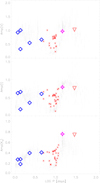 |
Fig. 5. Top: Bailey diagram of bulge and ω Cen T2Cs in the V band. Gray shows bulge BLHs, red crosses present bulge pWVs, and the other symbols are for ω Cen T2Cs and have the same meaning as in Figs. 1 and 4. The uncertainties of the light-curve amplitudes of ω Cen T2Cs are displayed as black error bars. Middle: same as in the top panel, but for the I band. The OGLE catalogs do not provide the uncertainties on the Amp(I), therefore we assumed an uncertainty of 0.05 mag. This is a conservative assumption because the median of the uncertainties on Amp(V) is 0.052 mag, and the I-band time series of OGLE have about one order of magnitude more points than the V-band time series. Bottom: same as in the top panel, but for the Ks band. |
We point out that the short-period BLHs of ω Cen are at the lower and upper edge of the distribution in the Bailey diagrams, especially the optical ones. This is the same behavior as we observed when we compared this with halo T2Cs. In passing we note that the peculiar WV stars (pWVs) are at fixed period brighter than canonical WV and are thought to belong to binary systems (Soszyński et al. 2008; Pilecki et al. 2017, 2018). The pWVs in the Bailey diagram appear to have optical amplitudes (Amp(V), Amp(I)) that are either similar to or larger than those of canonical WVs. In the NIR the trend is not so clear.
We adopted Amp(V), Amp(I) and Amp(Ks) to derive the amplitude ratios of T2Cs (see Fig. 6). Amp(I)/Amp(V) shows a clear linear trend with the period, and it is also interesting to note that the zero point (0.62) is almost identical to the Amp(I)/Amp(V) amplitude ratio of RRLs (0.63 ± 0.01 Braga et al. 2016). It would be tempting to adopt Amp(I)/Amp(V) to separate RRLs and T2Cs because of their different behavior (RRLs display a constant Amp(I)/Amp(V)). However, the intrinsic dispersion of the trend and the uncertainties on the amplitudes are larger than the difference of Amp(I)/Amp(V) between RRLs and T2Cs, especially at short periods (< 3 days), where RRLs disguised as T2Cs are to be searched for. The ratios involving the Ks-band amplitudes display a less clear behavior, with BLHs+WVS and RVTs following different trends. More precisely, both the Amp(Ks)/Amp(V) and Amp(Ks)/Amp(I) ratios increase with period in the BLH range, approach a steady value, and then decrease again in the 16−20 day range. However, we conservatively fit their distribution with a simple linear fit, also because the dispersion is quite large compared to the average ratio.
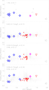 |
Fig. 6. Panel a: B over V amplitude ratios of GGC T2Cs. Black shows T2Cs from NGC 6388 and NGC 6441, and the other symbols have the same meaning as in Figs. 1 and 4. The solid red line denotes the average, and the dotted lines denote the 1σ dispersion. Panel b: I over V amplitude ratios of bulge and ω Cen T2Cs. The red line displays a linear fit. The symbols have the same meaning as in Fig. 5. Panel c: same as in panel b, but for Ks over V amplitude ratios. The red line displays a linear fit for log P < 1.3 and the average for log P > 1.3. Panel d: same as in panel b, but for Ks over I amplitude ratios. The red line displays a linear fit for log P < 1.3 and the average for log P > 1.3. |
Unfortunately, many RVTs are saturated in VVV data (Bhardwaj et al. 2017a; Braga et al. 2018a), therefore we have fewer points than for Amp(I)/Amp(V). The RVT ratios in the Ks band do not show any clear dependence on period, and they are lower than those of WVs. We ascribe the different behavior of the NIR amplitude ratios of RVTs to circumstellar dust. The long-wavelength excess light could explain the fact that in the NIR, the amplitudes are smaller than expected. Our referee noted that the dispersion in the optical/NIR amplitude ratios is larger than intrinsic errors and might be caused by a possible dependence on metal content. ω Cen T2Cs within 2σ follow the trends that we have found, especially for the Amp(I)/Amp(V) ratio, which has the tightest relation.
4. Period-luminosity relation
Type 2 Cepheids are distance indicators that are not as widely used as CCs and RRLs because they are not as numerous. For this reason, the calibration of their PL still lags that of RRLs and CCs. However, T2Cs in GGCs already proved to be crucial for understanding the difference between Population I and Population II stars (Baade 1956).
4.1. The NIR PLs of T2Cs in GGCs
Although not all clusters host T2Cs, these variables are quite iconic for GGCs and were named “cluster cepheids” until the 1950s. Matsunaga et al. (2006) performed an analysis of the NIR PL relations of the T2Cs in 23 GGCs. Our aim is to complement their sample and update the relations. For ω Cen, these authors had data only for V1, V29, and V48. Moreover, they adopted E(B − V) from the Harris catalog of GGCs (Harris 1996) and derived the true distance moduli (DM0) from the MV–[Fe/H] relation of HB stars, adopting VHB and [Fe/H] from the Harris catalog. However, not only does this catalog contain heterogeneous data that are mostly based on optical investigations, but the MV–[Fe/H] relation is prone to both nonlinearity and evolutionary effects (Caputo et al. 2000). Moreover, several GGCs are located in the Galactic bulge, and recent NIR investigations provide more reliable estimates.
We therefore collected DM0 and E(B − V) of GGCs from the more recent literature to derive the absolute magnitudes. When possible, we favored papers providing distance estimates based on PL relations of variable stars and on NIR data. This means that in the end, our absolute magnitudes are slightly different compared to those of Matsunaga et al. (2006). The degree of homogeneity is not complete, but is higher than that of the Harris catalog. All references are listed in Table 4.
Distance moduli and reddening of GCs.
Finally, we added V43, V60, V61, and V92 to the sample of Matsunaga et al. (2006), and replaced their mean magnitudes of V1, V29, and V48 with our own values because our light curves are better sampled.
The updated PL relations that we derived agree very well with those found by Matsunaga et al. (2006) (see Table 5). By comparing our Fig. 7 with Fig. 3 in Matsunaga et al. (2006), we note that the T2Cs in ω Cen that we have in common (V1, V29, and V48) follow the NIR PL relations even more closely. The only relevant difference is the position of NGC 6256 V1: in our figure, it is ∼0.6 mag brighter in all bands, meaning an offset larger than 3σ.
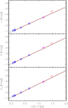 |
Fig. 7. Top: J-band PL relation of T2Cs in GGCs. Symbols for ω Cen are the same as in Figs. 1 and 4, the T2Cs from other GGCs are displayed as black crosses. The dashed black line displays the PL found by Matsunaga et al. (2006), and the dashed red line displays our own PL. Middle: same as in the top panel, but for the H-band PL relation. Bottom: same as in the top panel, but for the Ks-band PL relation. |
Empirical NIR PL relations of T2Cs in GGCs.
We point out that NGC 6256 is a bulge GGC, affected by high extinction, with a large uncertainty: E(B − V) ranges from 0.84 (Harris 1996) to 1.66 mag (Schlegel et al. 1998). Moreover, there is solid empirical evidence that the reddening in NGC 6256 most probably is differential (Valenti et al. 2007). We also verified that V1 is not blended in the IRSF JHKs images of Matsunaga et al. (2006). In the end, we cannot exclude the possibility that NGC 6256 V1 is a pWV. This type of object is slightly brighter than WVs and is likely to belong to a binary system (Soszyński et al. 2008). This would be the first pWV found in a GGC because pWVs have previously been identified in the MCs (Soszyński et al. 2008, 2010), in the field (κ Pav, Matsunaga et al. 2009), and in the bulge (Soszyński et al. 2017).
4.2. The PL transition from RRLs and T2Cs and distance determination
Figure 8 displays the PL relations of RRLs and T2Cs of ω Cen from the I to the Ks band (see Table 6). Because RRLs do not follow tight PL relations in passbands bluer than R (Catelan et al. 2004; Braga et al. 2015), we do not display the B and V PL relations. The R-band PL relations are not discussed because the light curves are hampered by poor or modest sampling. Theory and observations indicate that the PL relations of RRLs are mildly affected by metallicity (Marconi et al. 2015), while T2Cs are not (Di Criscienzo et al. 2007; Lemasle et al. 2015), therefore we decided to rescale the magnitudes of all ω Cen RRLs to the value they would have at the average metallicity of the sample. To do so, we adopted the theoretical metallicity coefficients of the PLs by Marconi et al. (2015, see their Table 6) and the new spectroscopic [Fe/H] estimates by Magurno et al. (2019). The rescaled magnitudes in a generic filter X (XFe) were determined as
![$$ \begin{aligned} X_{\rm Fe} = X - c \cdot (\mathrm{[Fe/H]} - \langle \mathrm{[Fe/H]}\rangle ) \end{aligned} $$](/articles/aa/full_html/2020/12/aa39145-20/aa39145-20-eq1.gif)
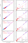 |
Fig. 8. IJHKs PL relations of RRLs and T2Cs in ω Cen. The symbols have the same meaning as in Figs. 1 and 4. Left panels: RRLs and T2Cs, and right panels: close-up of the period range of the transition between long-period RRab and BLHs. Red and purple lines show the PL relation of RRab and T2Cs, respectively. The dotted lines show the extension at longer and shorter periods of the RRab and T2Cs PL relations, respectively. The dispersions of the relations are displayed as bars in the lower right corner of the right panels. |
Empirical optical and NIR PL relations of T2Cs in ω Cen.
where c is the metallicity coefficient and ⟨[Fe/H]⟩ is the mean metallicity, calculated as log(⟨10[Fe/H]⟩), of ω Cen RRLs. These rescaled magnitudes were adopted to derive the PL relations of RRLs displayed in Fig. 8.
We note that with the only exception of the H-band, V29 (the WV) is always underluminous compared to the T2C relation, and V1 (the RVT) is always overluminous. If the PL relations of T2Cs were affected by metallicity in the same way as RRLs, we would expect the opposite behavior, based on the metal abundances by Gonzalez & Wallerstein (1994). This is further evidence that the effect of metallicity on the PL relations of T2Cs is negligible.
We note that in the JHKs bands, the long-period RRL stars follow both the RRab and the T2C relations. Most importantly, the coefficients of the RRab and T2C relations are the same within 1σ in the J and Ks bands, and they are practically identical in the H band. This means that RRab and T2Cs obey a common NIR PL relation, as has been suggested by Majaess (2010), based on optical data of GGCs and MCs, and by Navarrete et al. (2017), based on Ks-band photometry of ω Cen itself.
To estimate the DM0 of ω Cen, we adopted both our own empirical calibration of the NIR PL relation based on GGC T2Cs (Table 5) and as a comparison, that by Matsunaga et al. (2006)1 Finally, we derived the distance moduli that are listed in Table 7.
True distance moduli to ω Cen.
By following the referee’s suggestion, we obtained the Ks, J − Ks Period–Wesenheit (PW) relation, adopting the total-to-selective extinction ratio both by Cardelli et al. (1989,  = 0.69) and by Majaess et al. (2016,
  = 0.49) to derive the DM0. We found DM0 = 13.571 ± 0.073 ± 0.049 mag and DM0 = 13.718 ± 0.075 ± 0.052 mag, respectively. The use of different reddening laws affects the estimate of the true distance modulus at the level of ±1σ, but in opposite directions. Therefore we did not take the DMs derived from the PW into account and simply adopted the average value from the PLs as our final estimate of DM0. We note that the overall estimate agrees within 1σ with previous estimates based on RRLs and using the same photometry (Braga et al. 2016, 2018b).
5. Summary and final remarks
We have adopted optical (UBVRI) and NIR (JHKs) point spread function photometry of ω Cen (Braga et al. 2016, 2018b) and derived the pulsation properties (periods, mean magnitudes, light amplitudes, and light-curve Fourier coefficients) of its seven T2Cs. We discussed the transition between RRLs and T2Cs in detail by also using data from the OGLE-IV survey and adopting several diagnostics (CMD, Bailey diagram, Fourier coefficients, and light-curve template). We found that the period threshold at one day, which is commonly adopted to separate RRLs and T2Cs, is not universal. This was already evident in the literature (Sandage et al. 1994), but this problem has not been investigated for a long time. After 25 years, based on an unprecedented amount of data including the OGLE -IV time series (Udalski et al. 2015), we have obtained the results we list below.
Three main mechanisms severely hamper the reliability of the period threshold as a method for separating RRLs and T2Cs.
Evolutionary effects: RRLs with periods longer than one day, overlapping with the shortest-period T2Cs, are predicted by pulsation models for evolved objects approaching helium exhaustion (Marconi et al. 2015, 2018).
Helium abundance: Although there is no direct evidence of helium enhancement of the RRLs and T2Cs of ω Cen, pulsation models predict that helium-enhanced RRLs have periods longer than one day (Marconi et al. 2018). This means that helium-enhanced RRLs can also overlap in period with the shortest period T2Cs.
Period aliasing: The most severe periodicity alias for ground-based observations when various types of techniques are used to estimate periodicity (e.g., Lomb-Scargle, Phase Dispersion Minimization, string length) is at one day because of the daily cycle of telescope activity. The lack of variable stars around this period is at least in part due to this alias, which makes it more difficult to detect the correct period. Only OGLE (thanks to its huge number of observations) and Gaia (Gaia Collaboration 2016), the latter being a space telescope, easily overcome this limitation among the largest surveys. In the future, the LSST is also expected to be less affected by this period alias because its final time series will be extended.
To summarize, the period threshold is not universal, and when it is adopted, it brings an approximate separation. Based on the diagnostics discussed in Sect. 2.1 (especially the ϕ31 − log P diagram and the residuals from template light curves), we propose that V92 (P = 1.346 days) be reclassified as a candidate RRab. We also found that 15 bulge variables, previously classified as BLHs in the OGLE survey (Soszyński et al. 2017), are more similar to long-period RRab than to other T2Cs. Therefore we suggest that these variables be reclassified as candidate RRab stars.
We therefore suggest a more rigorous although less immediate approach to separating RRLs and T2Cs based on the evolutionary status of the star. We consider as RRLs all the pulsating stars of the RRL and Cepheid IS that are in their core helium-burning stage, regardless of their period. Only stars that have exhausted helium in their cores should be classified as T2Cs.
Unfortunately, it is hard to provide a solid diagnostic to follow this evolutionary criterion for several reasons. (i) The ZAHB and helium-exhaustion tracks in the CMD depend on metallicity and helium abundance. Moreover, each stellar evolutionary code generates slightly different tracks, depending on model assumptions (e.g., convection efficiency). In addition, a proper comparison with empirical data would require a supplementary spectroscopic investigation to estimate the [Fe/H] abundance of the T2Cs. (ii) Although the ϕ31 − log P diagram is very informative, we verified that the morphological subclasses of BLHs (the so-called AHB1, AHB2, and AHB3, where AHB1 are commonly associated with RRab) are not well separated in this diagram. Moreover, at least some dozen phase points are required for deriving a reliable estimate of the Fourier coefficients, which is not always the case for extensive surveys where variability is not among the main science cases.
We have studied the properties of the PL relations of RRLs and T2Cs. We found empirical evidence that RRab and T2Cs obey the same JHKs-band PL relations, thus confirming the preliminary working hypothesis by Majaess (2010). This has remarkable consequences for distance estimates and in turn for the setting of an extragalactic distance scale anchored only on Population II stars. The most severe limitation to the use of RRLs as distance indicators is their faintness, even though they are ubiquitous and very numerous. T2Cs are 1 to 5 mag brighter, meaning that they can be detected in both farther and more reddened environments. On the other hand, the use of T2Cs is hampered by their modest number (at least one order of magnitude smaller than RRLs). By virtue of the existence of a common PLs, RRLs and T2Cs might therefore be employed together, as if they were the same class of variable stars, and their respective weaknesses as distance indicators might thus be overcome. A more solid calibration based on more objects is needed, but this assumption still opens the path to adopting a RRL+T2C calibration of SNIa, leading to an independent estimate of H0.
Although at the time of writing, there is no possibility to calibrate the RRL+T2C NIR PL relations based on a large sample of both types of variables, upcoming instrumentation in the near future will provide this opportunity. First of all, WFIRST and JWST (Gardner et al. 2006) will provide NIR photometry of wide and shallow and narrow and deep areas, respectively. Moreover, the next Gaia data releases will provide not only more accurate parallaxes for a geometrical calibration, but also more extended time series. On the other hand, LSST (LSST Science Collaboration 2009) will provide an unprecedented wealth of time series in six passbands (ugrizy). These will be crucial for establishing more quantitative criteria to separate RRLs from T2Cs by using both the quoted diagnostics and eventually, the color-color curves (Diethelm 1983) for which an optimal coverage of the light curves in at least three passbands is required.
The coefficients in Table 5 were obtained by including ω Cen T2Cs. In principle, for a rigorous estimate of ω Cen distance we should rederive the coefficients of the NIR PL relations by removing ω Cen T2Cs from the sample discussed in Sect. 4.1. However, we confirmed that within the errors, the coefficients are the same regardless of whether ω Cen T2Cs are included in the sample.
Acknowledgments
We thank the anonymous refere for his/her valuable suggestions, which helped to improve the content and shape of the paper. V.F.B. acknowledges the financial support of the Istituto Nazionale di Astrofisica (INAF), Osservatorio Astronomico di Roma, and Agenzia Spaziale Italiana (ASI) under contract to INAF: ASI 2014-049- R.0 dedicated to SSDC. G.F. has been supported by the Futuro in Ricerca 2013 (grant RBFR13J716).
References
- Abolfathi, B., Aguado, D. S., Aguilar, G., et al. 2018, ApJS, 235, 42 [NASA ADS] [CrossRef] [Google Scholar]
- Baade, W. 1956, PASP, 68, 5 [CrossRef] [Google Scholar]
- Bailey, S. I. 1902, Ann. Harvard Coll. Obs., 38, 252 [Google Scholar]
- Baumgardt, H., Hilker, M., Sollima, A., & Bellini, A. 2019, MNRAS, 482, 5138 [Google Scholar]
- Beaton, R. L., Freedman, W. L., Madore, B. F., et al. 2016, ApJ, 832, 210 [Google Scholar]
- Beaton, R. L., Bono, G., Braga, V. F., et al. 2018, Space Sci. Rev., 214, 113 [CrossRef] [Google Scholar]
- Beaton, R. L., Seibert, M., Hatt, D., et al. 2019, ApJ, 885, 141 [NASA ADS] [CrossRef] [Google Scholar]
- Bekki, K., & Tsujimoto, T. 2019, ApJ, 886, 121 [CrossRef] [Google Scholar]
- Bellini, A., Piotto, G., Milone, A. P., et al. 2013, ApJ, 765, 32 [NASA ADS] [CrossRef] [Google Scholar]
- Benedict, G. F., McArthur, B. E., Feast, M. W., et al. 2011, AJ, 142, 187 [Google Scholar]
- Bhardwaj, A., Rejkuba, M., Minniti, D., et al. 2017a, A&A, 605, A100 [NASA ADS] [CrossRef] [EDP Sciences] [Google Scholar]
- Bhardwaj, A., Macri, L. M., Rejkuba, M., et al. 2017b, AJ, 153, 154 [NASA ADS] [CrossRef] [Google Scholar]
- Bono, G., Caputo, F., & Santolamazza, P. 1997a, A&A, 317, 171 [NASA ADS] [Google Scholar]
- Bono, G., Caputo, F., Cassisi, S., Incerpi, R., & Marconi, M. 1997b, ApJ, 483, 811 [NASA ADS] [CrossRef] [Google Scholar]
- Bono, G., Caputo, F., Castellani, V., & Marconi, M. 1997c, A&AS, 121, 327 [NASA ADS] [CrossRef] [EDP Sciences] [Google Scholar]
- Bono, G., Braga, V. F., Fiorentino, G., et al. 2020, A&A, 644, A96 [CrossRef] [EDP Sciences] [Google Scholar]
- Braga, V. F., Dall’Ora, M., Bono, G., et al. 2015, ApJ, 799, 165 [CrossRef] [Google Scholar]
- Braga, V. F., Stetson, P. B., Bono, G., et al. 2016, AJ, 152, 170 [NASA ADS] [CrossRef] [Google Scholar]
- Braga, V. F., Bhardwaj, A., Contreras Ramos, R., et al. 2018a, A&A, 619, A51 [NASA ADS] [CrossRef] [EDP Sciences] [Google Scholar]
- Braga, V. F., Stetson, P. B., Bono, G., et al. 2018b, AJ, 155, 137 [NASA ADS] [CrossRef] [Google Scholar]
- Braga, V. F., Contreras Ramos, R., Minniti, D., et al. 2019, A&A, 625, A151 [CrossRef] [EDP Sciences] [Google Scholar]
- Busso, G., Cassisi, S., Piotto, G., et al. 2007, A&A, 474, 105 [NASA ADS] [CrossRef] [EDP Sciences] [Google Scholar]
- Calamida, A., Zocchi, A., Bono, G., et al. 2020, ApJ, 891, 167 [CrossRef] [Google Scholar]
- Caldwell, C. N., & Butler, D. 1978, AJ, 83, 1190 [CrossRef] [Google Scholar]
- Caputo, F., Castellani, V., Marconi, M., & Ripepi, V. 2000, MNRAS, 316, 819 [Google Scholar]
- Cardelli, J. A., Clayton, G. C., & Mathis, J. S. 1989, ApJ, 345, 245 [NASA ADS] [CrossRef] [Google Scholar]
- Cassisi, S., Salaris, M., Anderson, J., et al. 2009, ApJ, 702, 1530 [NASA ADS] [CrossRef] [Google Scholar]
- Castellani, V., Calamida, A., Bono, G., et al. 2007, ApJ, 663, 1021 [NASA ADS] [CrossRef] [Google Scholar]
- Catelan, M., & Smith, H. A. 2015, Pulsating Stars (Weinheim: Wiley-VCH) [CrossRef] [Google Scholar]
- Catelan, M., Pritzl, B. J., & Smith, H. A. 2004, ApJS, 154, 633 [Google Scholar]
- Clement, C. M., Muzzin, A., Dufton, Q., et al. 2001, AJ, 122, 2587 [NASA ADS] [CrossRef] [Google Scholar]
- Clementini, G., Gratton, R. G., Bragaglia, A., et al. 2005, ApJ, 630, L145 [NASA ADS] [CrossRef] [Google Scholar]
- Constantino, T., Campbell, S. W., Lattanzio, J. C., & van Duijneveldt, A. 2016, MNRAS, 456, 3866 [NASA ADS] [CrossRef] [Google Scholar]
- Dalessandro, E., Salaris, M., Ferraro, F. R., et al. 2011, MNRAS, 410, 694 [NASA ADS] [CrossRef] [Google Scholar]
- Dawson, D. W. 1979, ApJS, 41, 97 [NASA ADS] [CrossRef] [Google Scholar]
- Di Criscienzo, M., Caputo, F., Marconi, M., & Cassisi, S. 2007, A&A, 471, 893 [NASA ADS] [CrossRef] [EDP Sciences] [Google Scholar]
- Diethelm, R. 1983, A&A, 124, 108 [NASA ADS] [Google Scholar]
- Diethelm, R. 1990, A&A, 239, 186 [Google Scholar]
- Fabrizio, M., Bono, G., Braga, V. F., et al. 2019, ApJ, 882, 169 [NASA ADS] [CrossRef] [Google Scholar]
- Ferraro, F. R., Messineo, M., Fusi Pecci, F., et al. 1999, AJ, 118, 1738 [NASA ADS] [CrossRef] [Google Scholar]
- Freedman, W. L., Madore, B. F., Hoyt, T., et al. 2020, ApJ, 891, 57 [Google Scholar]
- Gaia Collaboration (Prusti, T., et al.) 2016, A&A, 595, A1 [NASA ADS] [CrossRef] [EDP Sciences] [Google Scholar]
- Gaia Collaboration (Brown, A. G. A., et al.) 2018, A&A, 616, A17 [Google Scholar]
- Gardner, J. P., Mather, J. C., Clampin, M., et al. 2006, Space Sci. Rev., 123, 485 [NASA ADS] [CrossRef] [Google Scholar]
- Gautschy, A., & Saio, H. 1996, ARA&A, 34, 551 [NASA ADS] [CrossRef] [Google Scholar]
- Gingold, R. A. 1974, ApJ, 193, 177 [NASA ADS] [CrossRef] [Google Scholar]
- Gingold, R. A. 1985, Mem. Soc. Astron. It., 56, 169 [Google Scholar]
- Gonzalez, G., & Wallerstein, G. 1994, AJ, 108, 1325 [NASA ADS] [CrossRef] [Google Scholar]
- Harris, W. E. 1996, AJ, 112, 1487 [NASA ADS] [CrossRef] [Google Scholar]
- Helmi, A. 2020, ARA&A, 58, 205 [CrossRef] [Google Scholar]
- Helmi, A., Babusiaux, C., Koppelman, H. H., et al. 2018, Nature, 563, 85 [NASA ADS] [CrossRef] [Google Scholar]
- Ibata, R. A., Bellazzini, M., Malhan, K., Martin, N., & Bianchini, P. 2019, Nat. Astron., 3, 667 [NASA ADS] [CrossRef] [Google Scholar]
- Ivanov, V. D., Borissova, J., Alonso-Herrero, A., & Russeva, T. 2000, AJ, 119, 2274 [NASA ADS] [CrossRef] [Google Scholar]
- Jayasinghe, T., Stanek, K. Z., Kochanek, C. S., et al. 2019, MNRAS, 485, 961 [NASA ADS] [CrossRef] [Google Scholar]
- Johnson, C. I., & Pilachowski, C. A. 2010, ApJ, 722, 1373 [NASA ADS] [CrossRef] [Google Scholar]
- Johnson, C. I., Dupree, A. K., Mateo, M., et al. 2020, AJ, 159, 254 [CrossRef] [Google Scholar]
- Jurcsik, J., Clement, C., Geyer, E. H., & Domsa, I. 2001, AJ, 121, 951 [NASA ADS] [CrossRef] [Google Scholar]
- Kaisler, D., Harris, W. E., & McLaughlin, D. E. 1997, PASP, 109, 920 [NASA ADS] [CrossRef] [Google Scholar]
- Kaluzny, J., Olech, A., Thompson, I. B., et al. 2004, A&A, 424, 1101 [NASA ADS] [CrossRef] [EDP Sciences] [Google Scholar]
- Kodric, M., Riffeser, A., Hopp, U., et al. 2018, AJ, 156, 130 [CrossRef] [Google Scholar]
- Kovtyukh, V., Wallerstein, G., Yegorova, I., et al. 2018a, PASP, 130, 054201 [CrossRef] [Google Scholar]
- Kovtyukh, V., Yegorova, I., Andrievsky, S., et al. 2018b, MNRAS, 477, 2276 [CrossRef] [Google Scholar]
- Kruijssen, J. M. D., Pfeffer, J. L., Chevance, M., et al. 2020, MNRAS, 498, 2472 [CrossRef] [Google Scholar]
- Kunder, A., Salaris, M., Cassisi, S., et al. 2013, AJ, 145, 25 [CrossRef] [Google Scholar]
- Latour, M., Randall, S. K., Calamida, A., Geier, S., & Moehler, S. 2018, A&A, 618, A15 [CrossRef] [EDP Sciences] [Google Scholar]
- Lázaro, C., Arellano Ferro, A., Arévalo, M. J., et al. 2006, MNRAS, 372, 69 [NASA ADS] [CrossRef] [Google Scholar]
- Lee, Y. W., Joo, J. M., Sohn, Y. J., et al. 1999, Nature, 402, 55 [NASA ADS] [CrossRef] [Google Scholar]
- Lemasle, B., Kovtyukh, V., Bono, G., et al. 2015, A&A, 579, A47 [NASA ADS] [CrossRef] [EDP Sciences] [Google Scholar]
- LSST Science Collaboration (Abell, P. A., et al.) 2009, ArXiv e-prints [arXiv:0912.0201] [Google Scholar]
- Maas, T., Giridhar, S., & Lambert, D. L. 2007, ApJ, 666, 378 [NASA ADS] [CrossRef] [Google Scholar]
- Macri, L. M., Stanek, K. Z., Bersier, D., Greenhill, L. J., & Reid, M. J. 2006, ApJ, 652, 1133 [NASA ADS] [CrossRef] [Google Scholar]
- Magurno, D., Sneden, C., Bono, G., et al. 2019, ApJ, 881, 104 [CrossRef] [Google Scholar]
- Majaess, D. J. 2010, J. Am. Assoc. Var. Star Obs., 38, 100 [Google Scholar]
- Majaess, D. J. 2020, ApJ, 897, 13 [CrossRef] [Google Scholar]
- Majaess, D., Turner, D., & Lane, D. 2009, Acta Astron., 59, 403 [NASA ADS] [Google Scholar]
- Majaess, D., Turner, D., Dékány, I., Minniti, D., & Gieren, W. 2016, A&A, 593, A124 [NASA ADS] [CrossRef] [EDP Sciences] [Google Scholar]
- Marconi, M., & Minniti, D. 2018, ApJ, 853, L20 [NASA ADS] [CrossRef] [Google Scholar]
- Marconi, M., Bono, G., Caputo, F., et al. 2011, ApJ, 738, 111 [NASA ADS] [CrossRef] [Google Scholar]
- Marconi, M., Coppola, G., Bono, G., et al. 2015, ApJ, 808, 50 [NASA ADS] [CrossRef] [Google Scholar]
- Marconi, M., Bono, G., Pietrinferni, A., et al. 2018, ApJ, 864, L13 [CrossRef] [Google Scholar]
- Massari, D., Koppelman, H. H., & Helmi, A. 2019, A&A, 630, L4 [NASA ADS] [CrossRef] [EDP Sciences] [Google Scholar]
- Matsunaga, N., Fukushi, H., Nakada, Y., et al. 2006, MNRAS, 370, 1979 [Google Scholar]
- Matsunaga, N., Feast, M. W., & Menzies, J. W. 2009, MNRAS, 397, 933 [NASA ADS] [CrossRef] [Google Scholar]
- Matsunaga, N., Feast, M. W., Kawadu, T., et al. 2013, MNRAS, 429, 385 [NASA ADS] [CrossRef] [Google Scholar]
- Myeong, G. C., Vasiliev, E., Iorio, G., Evans, N. W., & Belokurov, V. 2019, MNRAS, 488, 1235 [NASA ADS] [CrossRef] [Google Scholar]
- Navarrete, C., Contreras Ramos, R., Catelan, M., et al. 2015, A&A, 577, A99 [NASA ADS] [CrossRef] [EDP Sciences] [Google Scholar]
- Navarrete, C., Catelan, M., Contreras Ramos, R., et al. 2017, A&A, 604, A120 [CrossRef] [EDP Sciences] [Google Scholar]
- Origlia, L., Rood, R. T., Fabbri, S., et al. 2007, ApJ, 667, L85 [NASA ADS] [CrossRef] [Google Scholar]
- Pietrinferni, A., Cassisi, S., Salaris, M., & Castelli, F. 2006, ApJ, 642, 797 [NASA ADS] [CrossRef] [Google Scholar]
- Pilecki, B., Gieren, W., Smolec, R., et al. 2017, ApJ, 842, 110 [NASA ADS] [CrossRef] [Google Scholar]
- Pilecki, B., Dervişoğlu, A., Gieren, W., et al. 2018, ApJ, 868, 30 [CrossRef] [Google Scholar]
- Planck Collaboration VI. 2020, A&A, 641, A6 [NASA ADS] [CrossRef] [EDP Sciences] [Google Scholar]
- Pojmanski, G. 1997, Acta Astron., 47, 467 [Google Scholar]
- Pritzl, B. J., Smith, H. A., Catelan, M., & Sweigart, A. V. 2002, AJ, 124, 949 [NASA ADS] [CrossRef] [Google Scholar]
- Riess, A. G., Casertano, S., Yuan, W., Macri, L. M., & Scolnic, D. 2019, ApJ, 876, 85 [NASA ADS] [CrossRef] [Google Scholar]
- Ripepi, V., Moretti, M. I., Marconi, M., et al. 2015, MNRAS, 446, 3034 [NASA ADS] [CrossRef] [Google Scholar]
- Ripepi, V., Molinaro, R., Musella, I., et al. 2019, A&A, 625, A14 [NASA ADS] [CrossRef] [EDP Sciences] [Google Scholar]
- Samus’, N. N., Kazarovets, E. V., Durlevich, O. V., Kireeva, N. N., & Pastukhova, E. N. 2017, Astron. Rep., 61, 80 [NASA ADS] [CrossRef] [Google Scholar]
- Sandage, A., Diethelm, R., & Tammann, G. A. 1994, A&A, 283, 111 [Google Scholar]
- Schlegel, D. J., Finkbeiner, D. P., & Davis, M. 1998, ApJ, 500, 525 [NASA ADS] [CrossRef] [Google Scholar]
- Shappee, B. J., Prieto, J. L., Grupe, D., et al. 2014, ApJ, 788, 48 [NASA ADS] [CrossRef] [Google Scholar]
- Sollima, A., Cacciari, C., & Valenti, E. 2006, MNRAS, 372, 1675 [Google Scholar]
- Soszyński, I., Udalski, A., Szymański, M. K., et al. 2008, Acta Astron., 58, 293 [NASA ADS] [Google Scholar]
- Soszyński, I., Udalski, A., Szymański, M. K., et al. 2010, Acta Astron., 60, 91 [NASA ADS] [Google Scholar]
- Soszyński, I., Udalski, A., Pietrukowicz, P., et al. 2011, Acta Astron., 61, 285 [NASA ADS] [Google Scholar]
- Soszyński, I., Udalski, A., Szymański, M. K., et al. 2014, Acta Astron., 64, 177 [NASA ADS] [Google Scholar]
- Soszyński, I., Udalski, A., Szymański, M. K., et al. 2017, Acta Astron., 67, 297 [NASA ADS] [Google Scholar]
- Soszyński, I., Udalski, A., Szymański, M. K., et al. 2018, Acta Astron., 68, 89 [NASA ADS] [Google Scholar]
- Soszyński, I., Udalski, A., Wrona, M., et al. 2019, Acta Astron., 69, 321 [Google Scholar]
- Stetson, P. B., Saha, A., Ferrarese, L., et al. 1998, ApJ, 508, 491 [NASA ADS] [CrossRef] [Google Scholar]
- Stetson, P. B., Braga, V. F., Dall’Ora, M., et al. 2014, PASP, 126, 521 [NASA ADS] [CrossRef] [Google Scholar]
- Strom, S. E., Strom, K. M., Rood, R. T., & Iben, I., Jr. 1970, A&A, 8, 243 [Google Scholar]
- Sweigart, A. V., Greggio, L., & Renzini, A. 1989, ApJS, 69, 911 [NASA ADS] [CrossRef] [Google Scholar]
- Tailo, M., Di Criscienzo, M., D’Antona, F., Caloi, V., & Ventura, P. 2016, MNRAS, 457, 4525 [NASA ADS] [CrossRef] [Google Scholar]
- Tailo, M., Milone, A. P., Marino, A. F., et al. 2019, ApJ, 873, 123 [CrossRef] [Google Scholar]
- Udalski, A., Szymański, M. K., & Szymański, G. 2015, Acta Astron., 65, 1 [NASA ADS] [Google Scholar]
- Valenti, E., Ferraro, F. R., & Origlia, L. 2007, AJ, 133, 1287 [NASA ADS] [CrossRef] [Google Scholar]
- Valenti, E., Ferraro, F. R., & Origlia, L. 2010, MNRAS, 402, 1729 [NASA ADS] [CrossRef] [Google Scholar]
- van Loon, J. T. 2008, Mem. Soc. Astron. It., 79, 412 [Google Scholar]
- Vasiliev, E. 2019, MNRAS, 484, 2832 [NASA ADS] [CrossRef] [Google Scholar]
- Wallerstein, G. 2002, PASP, 114, 689 [Google Scholar]
- Wallerstein, G., & Cox, A. N. 1984, PASP, 96, 677 [Google Scholar]
- Wallerstein, G., & Farrell, E. M. 2018, AJ, 156, 299 [CrossRef] [Google Scholar]
- Warren, P. R., & Harvey, G. M. 1976, MNRAS, 175, 129 [CrossRef] [Google Scholar]
- Woolley, R. 1966, The Observatory, 86, 76 [Google Scholar]
- Yuan, W., Fausnaugh, M. M., Hoffmann, S. L., et al. 2020, ApJ, 902, 26 [CrossRef] [Google Scholar]
- Zsoldos, E. 1998, Acta Astron., 48, 775 [NASA ADS] [Google Scholar]
Appendix A: Identification
We did not find any new T2C within our new data, therefore we considered only the seven sources in the Clement catalog (Clement et al. 2001) that are classified as Population II Cepheids by Kaluzny et al. (2004). We discuss the transition between long-period RRLs and BLHs in Sect. 2.1.
We retrieved all the seven T2Cs in our images by cross-matching our astrometric solution (with an accuracy of 0.1″, see Braga et al. 2016) with the coordinates from the Clement et al. (2001) catalog. We provide updated RA and Dec of the T2Cs of ω Cen in Table A.1. We matched our coordinates with the Gaia DR2 (Gaia Collaboration 2018) astrometric catalog and found that they all match within 0.12″, except for V43. Its Gaia coordinates are ∼2.8″ away from ours. However, V43 has no measurements in the BP and RP bands, and its Gaia astrometric solution has only two parameters (RA, Dec instead of the more accurate five-parameter (RA, Dec, μRA, μDec, and π), solution. Therefore we assume that the best coordinates for V43 are ours.
Astrometric properties and classification of the T2Cs in ω Cen.
Appendix B: Light curves
For the optical and NIR light curves we adopted the photometry by Braga et al. (2016, 2018b). For V1, we added photometry from the ASAS Survey (Pojmanski 1997).
By following a suggestion of the referee, we quantitatively verified the effect of blending. Figure B.2 displays the residuals of the H-band magnitudes of T2Cs and long-period RRLs with respect to the empirical PL (H) derived in Sect. 4.2, plotted versus the angular distance from the center of the cluster. The small sample and wide dispersion of the residuals do not allow us to reach firm conclusions. However, there is no clear trend, suggesting that within the errors, blending does not affect our estimates.
Figure B.1 displays the optical and NIR phased light curves of the T2Cs. Their periods are displayed in Table B.1 and were derived with the multiband approach described in Stetson et al. (2014), using both optical and NIR data. We did not find any significant difference between our periods and those in the Clement et al. (2001) catalog; the relative offsets are smaller than 5 × 10⁻⁴ for all the T2Cs.
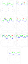 |
Fig. B.1. Top panels: optical light curves of the T2Cs of ω Cen. Purple sbows U, blue presents B, green shows V, red indicates R, and gray presents I. Names and periods are labeled in the top left and top right corners, respectively. Bottom panels: NIR light curves of the T2Cs of ω Cen. Blue shows J, green presents H, and red shows Ks. |
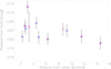 |
Fig. B.2. Residuals between measured and predicted H-band magnitude vs. angular distance from the center. Symbols have the same meaning as in Figs. 1 and 4. The bars represent the squared sum of photometric error plus the PL intrinsic dispersion. |
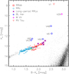 |
Fig. B.3. Optical-NIR(Ks, B − Ks) CMD of ω Cen (close-up of RRLs and T2Cs). The symbols have the same meaning as in Figs. 1 and 4. |
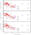 |
Fig. B.4. Bailey diagram of RRab and T2C stars in ω Cen. The symbols are the same as in Fig. B.3. Dashed lines represent the Oosterhoff 0 (Oo0, see Sect. 2.2), Oosterhoff I (OoI), and Oosterhoff II (OoII) loci of RRab stars. The Oo0 linear relation was derived by us in Sect. 2.2. OoI and OoII were adopted from Fabrizio et al. (2019). We rescaled the relations using the amplitude ratios provided by Braga et al. (2016). |
Optical mean magnitudes, amplitudes, and periods of the T2Cs in ω Cen.
NIR photometric properties of the T2Cs in ω Cen.
V1 does not show clear signs of alternating deep and shallow minima, typical of field RVTs with presumably intermediate mass. Moreover, it follows the same PL and PW relations as BLHs and WVs (see Sect. 4.1), which are the common features of GGC RVTs. According to Gonzalez & Wallerstein (1994), it is also metal poor ([Fe/H] = −1.77 dex) and highly enhanced in α elements ([α/Fe] > 0.4 dex). Therefore we consider V1 as a bona fide (low-mass and old) T2C.
V29 displays an almost sinusoidal light curve, typical of WVs with similar periods. It shows no signs of overluminosity, therefore it should be classified as a bona fide WV.
On the other hand, BLHs display varied light-curve morphologies, also at similar periods (see Fig. B.1). This is a known issue: Diethelm (1990) and Sandage et al. (1994) defined three different classes of T2Cs with periods shorter than three days: AHB1, AHB2, and AHB3 (see Appendix C). Because of the wide magnitude range covered by T2Cs and the accordingly broad range of evolutionary phases they experience, the classification of their light curve morphology and their correlation with physical parameters (stellar mass and chemical composition) is difficult. We inspected the light-curve morphologies of the BLHs in ω Cen. The results are the following, as summarized in Table A.1:
V43. The light curve of V43 displays a steep rising branch and a shallower decreasing branch. These are typical features of AHB1 stars.
V48. Its light curve is almost sinusoidal and does not look like any of the quoted morphological types. This is not unexpected because its period is ∼4.5 days, which is outside of the period range of the AHBs. It is the brightest BLH in ω Cen and the only one for which elemental abundances were derived (Gonzalez & Wallerstein 1994). Its low metallicity ([Fe/H] = −1.66) and the enhancement in α elements suggest that it is of the spectroscopic class UY Eri, recently proposed by Kovtyukh et al. (2018b).
V60. The light curve displays a flat maximum, typical of AHB3 stars.
V61. The light curve displays the typical bump of AHB2 class.
V92. The light curve displays a flat maximum, typical of AHB3 stars.
Our morphological classification matches that provided by Sandage et al. (1994) except for V60 and V92: they were classified as borderline AHB1 and anomalous Cepheid (AC). We rule out the possibility that V92 is an AC because based on its proper motion (see Table A.1), it is a cluster member (the proper motion of ω Cen is  = −3.24 ± 0.01 mas yr−1;
  = −6.73 ± 0.01 mas yr−1, Baumgardt et al. 2019), but does not follow the PL relation of cluster-member ACs, while it does follow the PL relation of cluster-member BLHs (see Sect. 4.2).
Appendix C: Variable subclasses above the horizontal branch
As Diethelm (1983) pointed out, variable AHB stars come in three different flavors, which were later labeled AHB1, AHB2, and AHB3 by Sandage et al. (1994). Their classification is based on the morphology of their optical light curves (see Fig. C.1).
 |
Fig. C.1. Sample-normalized I-band light curves of bulge AHB variables from OGLE-IV (Soszyński et al. 2017). |
AHB1 display saw-tooth RRab-like light curves (they were associated with RRLs by Diethelm (1983); AHB2 display a prominent secondary peak before the rising branch, and AHB3 stars display either a bump on the decreasing branch or a plateau that covers ∼20% of the pulsation cycle around the maximum light. The prototype BL Her itself is an AHB3 star with a solar-like metallicity, higher than the majority of T2Cs (Caldwell & Butler 1978; Maas et al. 2007). We verified that AHB1 and AHB3 variables are not well separated in the Bailey and the ϕ31 versus log P diagrams, but AHB2 are more easily detectable.
Appendix D: Light-curve template of long-period RRLs
To build the I-band light curve template of long-period RRLs, we selected 16 RRLs with periods between 0.97 and 1.00 days, that is, a sample that has no intersection with either the candidate RRLs or the short-period T2Cs groups. We normalized and cophased their I-band light curves by adopting the I-band amplitude and epoch of maximum provided by the OGLE collaboration. Their cumulated normalized light curve was fit with a eighth-order Fourier series (see Fig. D.1).
 |
Fig. D.1. Cumulated normalized light curve of long-period RRLs and the Fourier fit adopted as template light curve (red line). |
The coefficients are shown in Table D.1. We adopt this fit as the light-curve template for long-period RRLs.
Coefficients of the light-curve template.
All Tables
All Figures
|
Fig. 1. Optical (V vs. B − I) CMD of ω Cen. Light blue circles show RRc, red squares present RRab, purple asterisks indicate long-period-RRab, and blue diamonds show BLHs. Black and red lines display the ZAHB (solid) and helium-exhaustion (dotted) sequences for α-enhanced, helium-normal HB models (Pietrinferni et al. 2006) for two different metal contents: Z = 0.0006 ([Fe/H] = −1.84) and Z = 0.004 ([Fe/H] = −1.01). |
| In the text | |
|
Fig. 2. Top: ϕ21 − log P diagram of long-period RRLs and short-period T2Cs in ω Cen and Galactic bulge. Red dots present RRab, blue dots show T2Cs (I-band Fourier coefficients), and magenta dots present T2Cs (V-band Fourier coefficients). Middle: same as the top panel, but for the ϕ31 coefficients. The green box contains variables in the short-period T2C sample, the black box contains variables in the candidate RRL sample, and the light blue box contains variables in the RRL template sample. Bottom: bailey diagram of the same variables as in the top and middle panel. Light blue, black, and green cicles display variables in the short-period T2C, candidate RRL, and RRL template samples, respectively. |
| In the text | |
|
Fig. 3. Top: residuals of the I-band light curve of all candidate RRLs from the template fit. All the variables were phased with the period and epoch of maximum provided by OGLE, meaning that phase 0 is the phase of maximum brightness. Bottom: same as in the top panel, but for all the short-period T2Cs. |
| In the text | |
|
Fig. 4. Bailey diagram of T2Cs in the halo (gray points), and in ω Cen (same symbols as in Fig. 1, plus magenta star for the WV and an orange upside-down triangle for the RVT). |
| In the text | |
|
Fig. 5. Top: Bailey diagram of bulge and ω Cen T2Cs in the V band. Gray shows bulge BLHs, red crosses present bulge pWVs, and the other symbols are for ω Cen T2Cs and have the same meaning as in Figs. 1 and 4. The uncertainties of the light-curve amplitudes of ω Cen T2Cs are displayed as black error bars. Middle: same as in the top panel, but for the I band. The OGLE catalogs do not provide the uncertainties on the Amp(I), therefore we assumed an uncertainty of 0.05 mag. This is a conservative assumption because the median of the uncertainties on Amp(V) is 0.052 mag, and the I-band time series of OGLE have about one order of magnitude more points than the V-band time series. Bottom: same as in the top panel, but for the Ks band. |
| In the text | |
|
Fig. 6. Panel a: B over V amplitude ratios of GGC T2Cs. Black shows T2Cs from NGC 6388 and NGC 6441, and the other symbols have the same meaning as in Figs. 1 and 4. The solid red line denotes the average, and the dotted lines denote the 1σ dispersion. Panel b: I over V amplitude ratios of bulge and ω Cen T2Cs. The red line displays a linear fit. The symbols have the same meaning as in Fig. 5. Panel c: same as in panel b, but for Ks over V amplitude ratios. The red line displays a linear fit for log P < 1.3 and the average for log P > 1.3. Panel d: same as in panel b, but for Ks over I amplitude ratios. The red line displays a linear fit for log P < 1.3 and the average for log P > 1.3. |
| In the text | |
|
Fig. 7. Top: J-band PL relation of T2Cs in GGCs. Symbols for ω Cen are the same as in Figs. 1 and 4, the T2Cs from other GGCs are displayed as black crosses. The dashed black line displays the PL found by Matsunaga et al. (2006), and the dashed red line displays our own PL. Middle: same as in the top panel, but for the H-band PL relation. Bottom: same as in the top panel, but for the Ks-band PL relation. |
| In the text | |
|
Fig. 8. IJHKs PL relations of RRLs and T2Cs in ω Cen. The symbols have the same meaning as in Figs. 1 and 4. Left panels: RRLs and T2Cs, and right panels: close-up of the period range of the transition between long-period RRab and BLHs. Red and purple lines show the PL relation of RRab and T2Cs, respectively. The dotted lines show the extension at longer and shorter periods of the RRab and T2Cs PL relations, respectively. The dispersions of the relations are displayed as bars in the lower right corner of the right panels. |
| In the text | |
|
Fig. B.1. Top panels: optical light curves of the T2Cs of ω Cen. Purple sbows U, blue presents B, green shows V, red indicates R, and gray presents I. Names and periods are labeled in the top left and top right corners, respectively. Bottom panels: NIR light curves of the T2Cs of ω Cen. Blue shows J, green presents H, and red shows Ks. |
| In the text | |
|
Fig. B.2. Residuals between measured and predicted H-band magnitude vs. angular distance from the center. Symbols have the same meaning as in Figs. 1 and 4. The bars represent the squared sum of photometric error plus the PL intrinsic dispersion. |
| In the text | |
|
Fig. B.3. Optical-NIR(Ks, B − Ks) CMD of ω Cen (close-up of RRLs and T2Cs). The symbols have the same meaning as in Figs. 1 and 4. |
| In the text | |
|
Fig. B.4. Bailey diagram of RRab and T2C stars in ω Cen. The symbols are the same as in Fig. B.3. Dashed lines represent the Oosterhoff 0 (Oo0, see Sect. 2.2), Oosterhoff I (OoI), and Oosterhoff II (OoII) loci of RRab stars. The Oo0 linear relation was derived by us in Sect. 2.2. OoI and OoII were adopted from Fabrizio et al. (2019). We rescaled the relations using the amplitude ratios provided by Braga et al. (2016). |
| In the text | |
|
Fig. C.1. Sample-normalized I-band light curves of bulge AHB variables from OGLE-IV (Soszyński et al. 2017). |
| In the text | |
|
Fig. D.1. Cumulated normalized light curve of long-period RRLs and the Fourier fit adopted as template light curve (red line). |
| In the text | |
Current usage metrics show cumulative count of Article Views (full-text article views including HTML views, PDF and ePub downloads, according to the available data) and Abstracts Views on Vision4Press platform.
Data correspond to usage on the plateform after 2015. The current usage metrics is available 48-96 hours after online publication and is updated daily on week days.
Initial download of the metrics may take a while.