| Issue |
A&A
Volume 646, February 2021
|
|
|---|---|---|
| Article Number | A165 | |
| Number of page(s) | 10 | |
| Section | Extragalactic astronomy | |
| DOI | https://doi.org/10.1051/0004-6361/202038770 | |
| Published online | 22 February 2021 | |
Resolving the inner accretion flow towards the central supermassive black hole in SDSS J1339+1310⋆
1
Departamento de Física Moderna, Universidad de Cantabria, Avda. de Los Castros s/n, 39005 Santander, Spain
e-mail: This email address is being protected from spambots. You need JavaScript enabled to view it.
; This email address is being protected from spambots. You need JavaScript enabled to view it.
2
O.Ya. Usikov Institute for Radiophysics and Electronics, National Academy of Sciences of Ukraine, 12 Acad. Proscury St., 61085 Kharkiv, Ukraine
3
Institute of Astronomy of V.N. Karazin Kharkiv National University, Svobody Sq. 4, 61022 Kharkiv, Ukraine
4
Department of Physics, United States Naval Academy, 572C Holloway Rd., Annapolis, MD 21402, USA
5
Institute of Radio Astronomy of the National Academy of Sciences of Ukraine, 4 Mystetstv St., 61002 Kharkiv, Ukraine
Received:
26
June
2020
Accepted:
25
December
2020
Abstract
We studied the accretion disc structure in the doubly imaged lensed quasar SDSS J1339+1310 using r-band light curves and UV-visible to near-IR spectra from the first 11 observational seasons after its discovery. The 2009−2019 light curves displayed pronounced microlensing variations on different timescales, and this microlensing signal permitted us to constrain the half-light radius of the 1930 Å continuum-emitting region. Assuming an accretion disc with an axis inclined at 60° to the line of sight, we obtained log(r1/2/cm) = 15.4−0.4+0.93. We also estimated the central black hole mass from spectroscopic data. The width of the C IV, Mg II, and Hβ emission lines, and the continuum luminosity at 1350, 3000, and 5100 Å, led to log(MBH/M⊙) = 8.6 ± 0.4. Thus, hot gas responsible for the 1930 Å continuum emission is likely orbiting a 4.0 × 10⁸ M⊙ black hole at an r1/2 of only a few tens of Schwarzschild radii.
Key words: accretion / accretion disks / gravitational lensing: micro / gravitational lensing: strong / quasars: individual: SDSS J1339+1310 / quasars: supermassive black holes
Tables 1, 3 and 4 are only available at the CDS via anonymous ftp to cdsarc.u-strasbg.fr (130.79.128.5) or via http://cdsarc.u-strasbg.fr/viz-bin/cat/J/A+A/646/A165
© ESO 2021
1. Introduction
Microlensing-induced variability in gravitationally lensed quasars allows astronomers to determine the sizes of compact continuum-emission regions in distant active galactic nuclei (e.g. Wambsganss 1998). Hence, this extrinsic variability has become an extremely powerful tool, as evidenced by results for QSO 2237+0305 (e.g. Kochanek 2004; Eigenbrod et al. 2008; Mosquera et al. 2013). In particular, visible continuum light curves of a lensed quasar at redshift z ∼ 1 − 2 may provide radii for UV continuum sources in the accretion disc around its central supermassive black hole (SMBH). To gain a more complete perspective of the inner accretion flow, it is also necessary to measure the SMBH mass from spectroscopic data (e.g. Morgan et al. 2018, and references therein). For a Schwarzschild black hole, its mass defines the innermost stable circular orbit (ISCO) of the gas in the disc, and thus, it provides information about the relative sizes of UV continuum sources. Furthermore, using data for 11 lensed quasars, Morgan et al. (2010) found a physically relevant correlation between disc size and SMBH mass. The precision of this correlation continues to be improved by the addition of measurements from new lensed quasar systems (Morgan et al. 2018; Cornachione et al. 2020).
Inada et al. (2009) reported the discovery of a set of doubly imaged gravitationally lensed quasars, which included SDSS J1339+1310. The two images (A and B) of this quasar are located at the same redshift, zs = 2.231, while the early-type galaxy G at zl = 0.607 acts as a gravitational lens (Shalyapin & Goicoechea 2014; Goicoechea & Shalyapin 2016). It is also thought that stellar mass objects in G act as gravitational microlenses, strongly affecting image B (Shalyapin & Goicoechea 2014, henceforth Paper I). Thus, SDSS J1339+1310 is very well suited to the study of its central engine from visible continuum light curves and spectroscopic observations. In order to reproduce observed microlensing variations via numerical simulations, and measure the SMBH mass, reliable extinction and (macro)lens models are also required. These models should rely on robust observational constraints, some of which were presented in Table 1 of Paper I. In addition to the astro-photometric solution in the last column of that table, we simultaneously obtained the macrolens magnification1 ratio μB/μA = 0.175 ± 0.015 and the dust extinction ratio ϵG, B/ϵG, A = 1.33 ± 0.11 at 5500 Å in the G rest-frame using some emission line cores and narrow components of carbon emission lines that presumably come from very extended regions not affected by microlensing (linear extinction; Goicoechea & Shalyapin 2016, henceforth Paper II). In Paper II, we also measured the time delay  d (A is leading), which is a critical quantity for accurately isolating the microlensing-induced variability from the source quasar’s intrinsic variability.
In this paper, we mainly focus on the structure of the inner accretion flow in SDSS J1339+1310. Section 2 presents r-band light curves and UV-visible to near-IR (NIR) spectra spanning 11 years (2009−2019). Our extinction and lens models for the system are described in Sect. 3. Section 4 is devoted to determining the mass of the central SMBH, and the r–band microlensing variability and the size of the corresponding continuum source are discussed in Sect. 5. Our conclusions appear in Sect. 6. Throughout the paper, we use a flat cosmology with H0 = 70 km s−1 Mpc−1, ΩM = 0.3, and ΩΛ = 0.7 (Hinshaw et al. 2009).
2. Observational data
2.1. Light curves in the r band
Within the framework of the Gravitational LENses and DArk MAtter (GLENDAMA) project2, whose objective is to perform and analyse observations of a sample of ten gravitationally lensed quasars (Gil-Merino et al. 2018), we are conducting an r-band monitoring of SDSS J1339+1310 with the 2.0 m Liverpool Telescope (LT; Steele et al. 2004). Light curves basically covering the first visibility season after the discovery of the double quasar, as well as four additional seasons in 2012−2015, were presented in Paper II. Here, we add four new seasons of LT data (2016−2019) and combine our LT light curves with magnitudes from other facilities. It is noteworthy that these complementary data are used to fill the 2010−2011 gap in LT brightness records and improve the sampling in other monitoring years.
The updated light curves of SDSS J1339+1310 consist of 241 observing epochs (nights). On the LT, we used the RATCam Charge-Coupled Device (CCD) camera and the Sloan r filter with a central wavelength (CWL) of 6247 Å during 68 epochs, and the IO:O CCD camera (Sloan r filter with CWL = 6187 Å) during 145 epochs. The properties of both cameras, exposure times, and pre-processing tasks were described in Paper II. For the LT monitoring campaign between 2009 and 2019, the median value of the full-width at half-maximum (FWHM) of the seeing disc was  . The first part of the Panoramic Survey Telescope and Rapid Response System project (PS1; Chambers et al. 2016) also imaged the double quasar in the r band with CWL = 6215 Å. The PS1 Data Release 23 (Flewelling et al. 2020) included warp frames at six epochs over the 2011−2014 period. Despite the use of short exposures of only 40 s, the pixel scale of
  pixel−1 and good seeing conditions (median FWHM of
  ) yielded useful photometric data (see below).
We also used frames of the lens system taken with the 1.5 m Maidanak Telescope (MT) on six nights in July and December 2010. These observations were carried out with the SNUCAM camera and the Bessell R filter (CWL = 6462 Å; Im et al. 2010). SNUCAM uses a CCD detector with a  pixel−1 scale, and several 180 or 300 s exposures were obtained at each of the six epochs. Basic pre-processing tasks were then applied to MT frames: bias subtraction, trimming, flat fielding, and World Coordinate System mapping. The median FWHM was
  . In addition, the science archive of the National Optical Astronomy Observatory4 provides public access to frames of SDSS J1339+1310 taken with the ANDICAM instrument (DePoy et al. 2003) on the 1.3 m SMARTS Telescope (ST). We selected the R-band exposures (CWL = 6576 Å) at 16 epochs over the 2013−2016 period. ANDICAM has a
  pixel−1 scale, and three 300 s exposures are available for each observation night. These ST frames were conveniently pre-processed before starting photometry. The median FWHM for the 16 observing epochs was
  .
.
Our photometric technique is detailed in Paper II, but we give a brief outline of main steps here. We obtained quasar fluxes through point-spread function (PSF) fitting as well as the IRAF (Tody 1986, 1993) and IMFITFITS (McLeod et al. 1998) software programs. The photometric model consisted of two PSFs (images A and B), a de Vaucouleurs profile convolved with the PSF (light distribution of G) and a constant sky background, and it was applied to all LT, PS1, MT, and ST frames. The Sloan Digital Sky Survey (SDSS) r-band magnitude of a reference star was used for calibrating quasar magnitudes, and typical errors of new LT data were estimated from root-mean-square deviations between magnitudes on consecutive nights (see Paper II). MT errors were derived from standard deviations of magnitudes on each observation night, while we adopted the typical errors in LT records as the PS1 and ST photometric uncertainties. The 11-year light curves are available in Table 1 at the CDS: Column 1 lists the observing date (MJD−50 000), Cols. 2−3 give magnitudes and magnitude errors of A, and Cols. 4−5 give magnitudes and magnitude errors of B. These curves are also displayed in Fig. 1. Although we mostly use observations in standard r bands (in 219 out of 241 epochs), there are data at slightly redder wavelengths in 22 epochs. This results in an effective, weighted average wavelength of 6237 Å, which translates to a UV continuum emission at 1930 Å. We also note that the LT data are in reasonably good agreement with those from PS1 and ST.
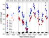 |
Fig. 1. Light curves of SDSS J1339+1310AB from its discovery to 2019. These r-band brightness records of the two quasar images are based on observations from four different facilities that are labelled as LT, MT, ST, and PS1 (see main text). Magnitudes of a field star are offset by +2.0 (triangles) to facilitate comparison with strong quasar variations. Dates of spectroscopic observations are marked by vertical dotted lines. |
The light curves over the full observing period 2009−2019 were initially used to cross-check the time delay measured in Paper II. In Appendix A, we confirm the delay based on a shorter monitoring period and show that the adopted error bar is very conservative.
2.2. UV-visible-NIR spectra
Spectroscopic observations of SDSS J1339+1310 were also performed between 2009 and 2019. Main details are incorporated into Table 2, and observing epochs are indicated in Fig. 1. The calibrated SDSS-BOSS spectra are publicly available in the SDSS database5. However, the BOSS spectrograph collected light into a 2″-diameter optical fibre (Dawson et al. 2013), which was centred on image A in the first epoch and on image B in the second. Hence, the two-epoch observations do not provide clean spectra of A or B. For instance, in the first epoch, although the spectral energy distribution mainly corresponds to A, a significant contribution of B and the lensing galaxy is also expected. We also conducted long-slit spectroscopy with the GTC, the TNG, and the NOT as part of the GLENDAMA project. The GTC-OSIRIS observations allowed us to resolve A, B, and G, and accurately extract their individual spectra (Paper I; Paper II). Using the R500R grism, the C IV emission line in quasar spectra appears close to its blue edge, whereas the Mg II emission line is located on its red edge. The C IV emission of the quasar is, however, seen in the central part of the R500B grism wavelength range. Additionally, our spectroscopic follow-up of both quasar images with NOT-ALFOSC and TNG-NICS, provided relatively noisy shapes for the C IV emission line and the first detection of Hα emission. These recent spectra will be presented in a future paper and not further considered here.
Spectroscopic observations in the 2009−2019 period.
The HST Data Archive6 also contains slitless spectroscopy of SDSS J1339+1310 with the WFC3 instrument. The observations were made using the G280 grism in the UVIS channel, and were presented by Lusso et al. (2018). Unfortunately, Lusso et al. (2018) only displayed resulting spectra for the two quasar images in their Fig. 2. Thus, we downloaded the HST-WFC3-UVIS original data and then extracted the quasar spectra that are plotted in Fig. 2. The overall shape of +1st order spectra (labelled as A+ and B+) agrees with that of −1st order ones (A− and B−). However, the throughput of the G280 grism is higher for the +1st order, and the associated spectra are less noisy. We accordingly take A+ and B+ as our final data. These HST-WFC3-UVIS spectra are available in tabular format at the CDS: Table 3a includes wavelengths in Å (Col. 1), and fluxes and flux errors of A in 10−17 erg cm−2 s−1 Å−1 (Cols. 2 and 3), while Table 3b includes wavelengths in Å (Col. 1), and fluxes and flux errors of B in 10−17 erg cm−2 s−1 Å−1 (Cols. 2 and 3). The spectral energy distributions show the C IV emission line around 5000 Å (∼1550 Å in the quasar rest-frame).
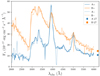 |
Fig. 2. HST-WFC3-UVIS spectra of SDSS J1339+1310AB in February 2016. The first order spectra are A+ and B+ (+1st order data), as well as A− and B− (−1st order data). Fluxes from LT r-band frames on 14 February 2016 are also shown for comparison purposes. |
We also downloaded and analysed observations in the three arms (UVB, VIS, and NIR) of VLT-X-shooter (Vernet et al. 2011). These are publicly available at the ESO Science Archive Facility7, and details on the observing programme are given in Table 2. For each of the two epochs, we used the 2700 (3 × 900) s exposure and a three-component fitting to resolve the spectra of A, B, and G. Our multi-component extraction technique is robust and has been recently applied to some lens systems (e.g. Sluse et al. 2007; Shalyapin & Goicoechea 2017; Goicoechea & Shalyapin 2019). The model we used can be described in a nutshell as follows: three 1D Moffat profiles in the spatial direction for each wavelength bin. Telluric absorption in the VIS and NIR arms was also corrected via the Molecfit software (Smette et al. 2015; Kausch et al. 2015). Final calibrated spectra of A, B, and G on 6 April 2017 are available at the CDS: Table 4 contains wavelengths in Å (Col. 1), fluxes and flux errors of A (Cols. 2 and 3), fluxes and flux errors of B (Cols. 4 and 5), and fluxes and flux errors of G (Cols. 6 and 7). The wavelength coverage ranges from 3050−20 700 Å (UVB, VIS, and NIR arms), and the fluxes and their errors are expressed in units of 10−17 erg cm−2 s−1 Å−1. These VLT-X-shooter spectra are also shown in Fig. 3. In addition to C IV emission of the quasar in the UVB arm spectra (top panel), Mg II and Hβ emissions are also seen around 9000 Å (∼2800 Å in the quasar rest-frame; middle panel) and 15 700 Å (∼4860 Å in the quasar rest-frame; bottom panel), respectively.
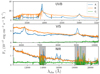 |
Fig. 3. VLT-X-shooter spectra of SDSS J1339+1310ABG in April 2017. The fluxes in the UVB, VIS, and NIR arms are depicted in the top, middle, and bottom panels, respectively. Grey highlighted regions display very noisy behaviours that are related to strong atmospheric absorption. |
3. Extinction and lens models
The position on the sky of SDSS J1339+1310 was used to estimate its extinction in the Milky Way at three wavelengths of interest. Based on the results of Schlafly & Finkbeiner (2011), the NASA/IPAC Extragalactic Database8 provided Milky Way transmission factors (ϵMW) of 0.93 at 4362 Å, 0.98 at 9693 Å, and 0.99 at 16 478 Å. These wavelengths correspond to 1350, 3000, and 5100 Å in the quasar rest-frame (see Sect. 4). While the Galaxy produces equal extinction in both quasar images, the lensing galaxy gives rise to a differential extinction between images. According to Paper II, emission lines in GTC-OSIRIS spectra and a linear extinction law in G (e.g. Prévot et al. 1984) lead to a dust extinction ratio (ratio between the transmission of B and that of A) of 1.33 ± 0.11 at 5500 Å in the lens rest-frame. Additionally, GTC-OSIRIS and VLT-X-shooter spectra indicate that Mg II absorption at the lens redshift is much stronger in A than in B. Therefore, it is reasonable to assume that the lens galaxy’s dust essentially affects image A, which translates to transmission factors (ϵG, A) of 0.56 ± 0.09, 0.77 ± 0.06, and 0.86 ± 0.04 for light emission at 1350, 3000, and 5100 Å, respectively (adopting an achromatic transmission factor ϵG, B = 1 for image B).
We also modelled the (macro)lensing mass using observational constraints in previous papers. We took the image positions, and the galaxy position, effective radius, ellipticity, and position angle in the fifth column of Table 1 of Paper I as constraints. The image fluxes were also considered to derive lens models. These fluxes are consistent with the macrolens magnification ratio measured in Paper II (see Sect. 1). The overall set of constraints allowed us to fit 11 free parameters with d.o.f. = 0, where ‘d.o.f.’ denotes the degrees of freedom. We used the GRAVLENS/LENSMODEL software (Keeton 2001), adopting a gravitational lens scenario that consists of three components. De Vaucouleurs (DV) and Navarro-Frenk-White (NFW; e.g. Navarro et al. 1996, 1997) mass profiles describe the stellar (light traces mass) and dark components of the main deflector G, whereas an external shear (ES) accounts for additional deflectors.
The sequence of DV+NFW+ES models started by assuming that all mass of G is traced by light, namely constant mass-to-light ratio model. The free parameters of such a model were the position, mass scale, effective radius, ellipticity, and position angle of the DV profile, the strength and direction of the ES, and the position and flux of the source quasar. By progressively decreasing the luminous component of G and adding a concentric dark matter halo, we completed a sequence of ten realistic lens models with f* ranging between 1.0 and 0.1, where f* is the mass of G in stars (DV profile) relative to its maximum value in the absence of a dark matter halo (we note that f* was called fM/L in several previous papers; e.g. Morgan et al. 2018; Cornachione et al. 2020). For the f* < 1 models, the free parameters were the common position, ellipticity, and position angle for both components of G (DV and NFW profiles), the effective radius of the DV profile, the mass scale of the NFW profile, the strength and direction of the ES, and the position and flux of the source quasar.
Some local parameters (at image positions) of the DV+NFW+ES models are shown in Table 5. The last three columns of Table 5 give the magnification factor of A and B for each time delay, so we took the measured delay ( d; Paper II, and discussion in Appendix A) as an additional constraint to estimate reliable intervals for μA and μB. First, results for the models in the range 0.6 ≤ f* ≤ 0.8 were used to construct power-law cross-correlations between magnifications and delays. If y = μA (or μB) and x = ΔtAB, we derived laws y ∝ x−α, where the power-law index is α ≈ 2. Second, these x–y relationships and the extreme values of the measured delay interval (x = 41 and 52 d) led to μA = 9.4 ± 2.2 and μB = 1.6 ± 0.4.
DV+NFW+ES lens models.
4. Black hole mass
For a given broad emission line, it is thought that the line-emitting gas is distributed within the gravitational potential of the central SMBH, so there is a relationship between its motion, the size of the region, and the SMBH mass (MBH; e.g. Vestergaard & Peterson 2006, and references therein). The gas motion is responsible for the emission-line width, while the radius of the line-emitting region scales roughly as the square root of the continuum luminosity (e.g. Koratkar & Gaskell 1991; Bentz et al. 2009). Hence, we aimed to use the single-epoch spectra of SDSS J1339+1310 in Table 2 to measure the black hole mass of the quasar. Although there are spectra for the two quasar images, image B is strongly affected by microlensing. Thus, we only considered image A when estimating MBH. We were primarily interested in the width of the C IV, Mg II, and Hβ emission lines, as well as the continuum flux for emissions at 1350, 3000, and 5100 Å (e.g. Vestergaard & Peterson 2006; Vestergaard & Osmer 2009). After the de-redshifting of the observed spectra of A to the quasar rest-frame, λrest = λobs/(1 + zs), if the continuum flux Fcont, A(λrest) is in 10−17 erg cm−2 s−1 Å−1 and the corresponding luminosity Lcont(λrest) is in erg s−1, then both quantities are related through the equation
 (1)
(1)
All factors in the denominator of Eq. (1) are discussed in Sect. 3.
The C IV emission line is well resolved in the GTC-OSIRIS-R500B spectrum of image A. In Fig. 4 of Paper II, we presented a multi-component decomposition of its profile in both images. For clarity, the carbon line profile in A is also depicted in the top panel of Fig. 4. After subtracting the local continuum, the residual signal is modelled as a sum of three Gaussian contributions. We focused on the C IV total (broad + narrow) emission line and calculated the square root of its second moment (σline; Peterson et al. 2004). The line width was then estimated from the spectral resolution-corrected line dispersion  km s−1. Moreover, the continuum flux at λrest = 1350 Å in May 2014 reached a level of 5.9 × 10⁻¹⁷ erg cm−2 s−1 Å−1, that is Fcont,A(1350 Å) = 5.9. We additionally considered the HST-WFC3-UVIS spectrum of A and analysed the region around the C IV line (see the bottom panel of Fig. 4). Thus, we obtained an independent line width σl = 4294 km s−1 based on HST data. Despite the fact that both spectra (GTC and HST) yield similar values of σl, the Fcont,A(1350 Å) values in the two observing epochs were very different. The continuum flux in February 2016 was Fcont,A(1350 Å) = 15.6. A dramatic change in the r-band flux between May 2014 (minimum level) and February 2016 (maximum level) is also seen in Fig. 1. From Eq. (1), accounting for uncertainties in the dust extinction and macrolens magnification of image A, we found log[Lcont(1350 Å)] = 45.30 ± 0.13 (GTC) and 45.72 ± 0.13 (HST).
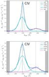 |
Fig. 4. Multi-component decomposition of the C IV line profile in SDSS J1339+1310A. The profile is decomposed into three Gaussian components: C IV broad + C IV narrow + He II complex. The grey rectangles highlight the two spectral regions that we used to remove a linear continuum under the emission line, and the vertical dotted lines correspond to the centres of the Gaussians. Top panel: GTC-OSIRIS-R500B data in May 2014, while bottom panel: HST-WFC3-UVIS data in February 2016. |
Vestergaard & Peterson (2006) derived equations for estimating the central black hole mass in a quasar from the C IV line width and Lcont(1350 Å), and we used their Eq. (8) to obtain C IV-based masses. The spectral observations in May 2014 (GTC) and February 2016 (HST) led to log[MBH(C IV)/M⊙ = 8.62 ± 0.33 and 8.91 ± 0.33, respectively. We have not considered uncertainties generated by errors in σl and Lcont(1350 Å) since the uncertainty in log[MBH(C IV)/M⊙] is dominated by an intrinsic scatter of ±0.33 dex rather than contributions from such errors. An error of 100 km s−1 in σl propagates to ±0.02 dex in log[MBH(C IV)/M⊙], whereas the uncertainties in Lcont(1350 Å) propagate to ±0.07 dex in the logarithm of the mass. Typical mass logarithms of 8.56 (GTC) and 8.83 (HST) were also inferred from Eq. (2) of Park et al. (2013).
Although both C IV-based masses are consistent within errors, and this would permit us to ‘confidently’ calculate the average, we carefully analysed the Mg II and Hβ emission lines in the VLT-X-shooter spectrum of A in April 2017. These VLT observations were made at an epoch for which the r-band flux reached an intermediate level (see Fig. 1), and therefore they may help to decide whether one of the two C IV-based estimates is relatively biased or not. In Fig. 5, we show multi-component decompositions of the Mg II and Hβ profiles (see the caption for details). First, we measured FWHM(Mg II) = 3984 km s−1 and Fcont,A(3000 Å) = 2.3. In addition, Eq. (1) provided the relevant continuum luminosity at 3000 Å, namely log[Lcont(3000 Å)] = 45.08 ± 0.11. Using Eq. (1) of Vestergaard & Osmer (2009) at λrest = 3000 Å, Eq. (10) of Wang et al. (2009), and Eq. (3) of Shen & Liu (2012), we obtained typical log[MBH(Mg II)/M⊙] values ranging between 8.58 and 8.70, in good agreement with those from the C IV line width and Lcont(1350 Å) in the GTC spectrum taken in May 2014.
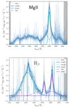 |
Fig. 5. Multi-component decomposition of the Mg II and Hβ line profiles in SDSS J1339+1310A. The data correspond to VLT-X-shooter observations in April 2017. The original wavelength bins contain a very noisy signal (lighter blue), so a nine-point median filter is used to smooth original data (darker blue). In the top panel, after subtracting a power-law continuum, the residual signal is modelled as a sum of two contributions, i.e. Mg II broad emission (Gaussian curve around the vertical dotted line) and Fe II pseudo-continuum. There is no evidence of a Mg II narrow line or an additional very broad component. The continuum windows at 2195−2215 Å and 3020−3070 Å are highlighted using grey rectangles, and the Fe II pseudo-continuum is created from the Fe II template of Tsuzuki et al. (2006) convolved with a Gaussian function to account for the Doppler broadening of Fe II lines. Bottom panel: decomposition in the spectral region around the Hβ emission. The grey rectangle highlights one of the two windows that we used to remove a power-law continuum under emission lines (3790−3810 Å and 5080−5100 Å; Kuraszkiewicz et al. 2002). The residual signal is decomposed into four Gaussian components: Hβ broad + Hβ narrow + [O III] doublet, plus the Fe II contribution from two individual lines in the spectral range 4750−5100 Å (e.g. Kovačević et al. 2010). Vertical dotted lines show the centres of the four Gaussians. |
From the decomposition in the bottom panel of Fig. 5 and Eq. (1), we also derived FWHM(Hβ) = 4928 km s−1, Fcont,A(5100 Å) = 0.53, and log[Lcont(5100 Å)]] = 44.61 ± 0.11. Following the prescription of Vestergaard & Peterson (2006), we only used the broad component of the Hβ emission to determine FWHM(Hβ). The FWHM(Hβ) and log[Lcont(5100 Å)] values yielded log[MBH(Hβ)/M⊙] = 8.60 ± 0.43 (Eq. (5) of Vestergaard & Peterson 2006), indicating an excellent agreement between the new measurement and log[MBH(C IV)/M⊙] from GTC data. We finally adopted log(MBH/M⊙) = 8.6 ± 0.4. This interval encompasses all our black-hole mass measurements from GTC and VLT spectra.
5. Accretion disc size from microlensing variability
We analysed the r-band light curves using the Monte Carlo analysis technique in Kochanek (2004). The method is fully described in that paper, but we provide a brief summary here. Using the convergence κ, convergence due to stars κ*, shear γ, and shear position angle θγ from each of the models in our sequence (see Table 5), we generated a set of 40 magnification patterns per macro model to represent the microlensing conditions at the location of each lensed image. Our model sequence has 10 macro models in the range 0.1 ≤ f* ≤ 1.0 (see Sect. 3), so we generated a total of 400 sets of magnification patterns.
Each of the 400 realisations was generated randomly using the inverse ray-shooting technique as described by Kochanek et al. (2006), the distribution of stellar masses for which were drawn from the Galactic bulge IMF of Gould (2000) in which dN(M)/dM ∝ M−1.3. The square magnification patterns represent a region 40 rE on a side, where rE is the source-plane projection of the Einstein radius of a 1 M⊙ star. With dimensions of 8192 × 8192 pixels, each pixel represents a physical distance of 1.60 × 10¹⁴⟨M*/M⊙⟩1/2 cm on the source plane, where ⟨M*⟩ is the mean mass of a lens galaxy star.
We convolved the magnification patterns with a simple Shakura & Sunyaev (1973) thin disc model for the surface brightness profile of the accretion disc at a range of source sizes  . The quantity
  is a thin disc scale radius where the hat indicates that the distance is being reported in ‘Einstein units’ in which quantities are scaled by a factor of the mean mass of a star in the lens galaxy. For example, converting a scale radius or velocity in Einstein units into a physical unit is accomplished using
  and
and  , respectively.
In essence our technique is an attempt to reproduce the observed microlensing variability using a realistic model for conditions in the lens galaxy. We run our model magnification patterns by a range of model source sizes on a range of trajectories in an attempt to fit the observed data. According to Bayes’ theorem, the likelihood of the set of physical ξp and trajectory ξt parameters given the data D is
 (2)
(2)
where P(ξt) and P(ξp) are the prior probabilities for the trajectory and physical variables, respectively. In a given trial, we chose the velocity randomly from the uniform logarithmic prior ![Mathematical equation: $ 1.0 \leq \log[\hat{v}_{\mathrm{e}} / ({\langle M_*/{M}_\odot \rangle}^{1/2} \, \mathrm{km \, s^{-1}})] \leq 5.0 $](/articles/aa/full_html/2021/02/aa38770-20/aa38770-20-eq18.gif) . We evaluated the goodness-of-fit with the chi-square statistic in real time during each trial, and for computational efficiency we aborted and discarded any fit with χ2/d.o.f. ≥ 1.6 since they do not contribute significantly to the Bayesian integrals. We attempted 107 Monte Carlo fits per set of magnification patterns for a grand total of 4 × 10⁹ trials. Of those trials, ∼105 met our χ2 threshold, and the remainder of our analysis was performed on those solutions. In Fig. 6, we display examples of five good fits to the observed microlensing variability.
. We evaluated the goodness-of-fit with the chi-square statistic in real time during each trial, and for computational efficiency we aborted and discarded any fit with χ2/d.o.f. ≥ 1.6 since they do not contribute significantly to the Bayesian integrals. We attempted 107 Monte Carlo fits per set of magnification patterns for a grand total of 4 × 10⁹ trials. Of those trials, ∼105 met our χ2 threshold, and the remainder of our analysis was performed on those solutions. In Fig. 6, we display examples of five good fits to the observed microlensing variability.
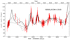 |
Fig. 6. Image Br-band light curve from the LT shifted by the 47-d time delay and subtracted from the contemporaneous magnitude of image A, i.e. mA(t)−mB(t + 47 d) (equivalent to a ratio in flux units), leaving only variability that is not intrinsic to the source itself. Plotted in black are five good fits to the microlensing variability from our Monte Carlo routine. |
We generated a statistical prior for the effective velocity between source, lens and observer using four components. We found the transverse velocity of the observer by calculating the northern (vO, n = −110.7 km s−1) and eastern (vO, e = −218.5 km s−1) components of the CMB dipole across the line of sight to the target. Following Bolton et al. (2008), we estimated the velocity dispersion σ* = 379 km s−1 in the lens galaxy using the monopole term of its gravitational potential. We estimated the peculiar velocity of source and lens using their redshifts, following the prescription of Mosquera & Kochanek (2011). Using the technique presented in Kochanek (2004), we combined the velocities to generate a probability density for the effective velocity (see the left panel of Fig. 7). Also shown in the left panel of Fig. 7 is the probability density for the effective velocity in Einstein units  yielded by marginalising over the other variables in the set of successful solutions from the Monte Carlo run
 (3)
(3)
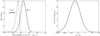 |
Fig. 7. Distributions for the effective source velocity and mean microlens mass. Left panel: probability density for the effective velocity |


where  is the probability of fitting the data in a particular trial, P(p) sets the priors on the microlensing variables ξp & ξt, and
  is the (uniform) prior on the effective velocity. The total probability is then normalised so that
  . We carried out an analogous Bayesian integral to find the probability density for the source size in Einstein units,
  , which we display in the left panel of Fig. 8.
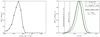 |
Fig. 8. Accretion disc structure in SDSS J1339+1310. Left panel: probability density for the source size in Einstein units (⟨M*/M⊙⟩1/2 cm). The distribution levels off at ∼2 × 1014 cm since the pixel scale in our magnification patterns is 1.6 × 1014 cm. All solutions become equally likely below that size scale. Right panel: probability density for the half light radius of the continuum-emission region in SDSS J1339+1310 at λrest = 1930 Å assuming an inclination angle cos i = 0.5. The solid black curve was derived by convolving our probability density for ⟨M*⟩ (right panel of Fig. 7) with that of |

Now, to convert our result from Einstein units to true physical units, we developed a probability density for the mean microlens mass ⟨M*⟩ (see the right panel of Fig. 7) by convolving the prior on ve with the probability density on  from the simulation since
  . To find the probability density for the source size in physical units, dP(rs)/d log rs, we convolved the probability density for ⟨M*⟩ with that of
  . Assuming an inclination angle of 60°, we display the resulting distribution for the half-light radius (r1/2) in the right panel of Fig. 8. In Fig. 8, we also show the probability density for r1/2 using an assumed uniform prior on the mean microlens mass 0.1 ≤ ⟨M*/M⊙⟩ ≤ 1.0. While the two results are fully consistent, we promote the measurement without the uniform mass prior, the expectation value for which is
 ![Mathematical equation: $ \log\{(r_{1/2}/\mathrm{cm})[\cos i/0.5]^{1/2}\} = 15.4^{+0.3}_{-0.4} $](/articles/aa/full_html/2021/02/aa38770-20/aa38770-20-eq33.gif) . This measurement is the half-light radius of the quasar continuum source at the rest-frame effective wavelength λrest = 1930 Å (see the end of Sect. 2.1).
. This measurement is the half-light radius of the quasar continuum source at the rest-frame effective wavelength λrest = 1930 Å (see the end of Sect. 2.1).
We also investigated the impact of uncertainty in the time delay on our measured microlensing sizes. We repeated our microlensing analysis at both the lower and upper 1σ bounds of the time delay, 41 and 52 d. We found size measurements of ![Mathematical equation: $ \log\{(r_{1/2}/\mathrm{cm})[\cos i/0.5]^{1/2}\}\,{=}\,15.5^{+0.3}_{-0.4} $](/articles/aa/full_html/2021/02/aa38770-20/aa38770-20-eq34.gif) and log{(r1/2/cm)
and log{(r1/2/cm) ![Mathematical equation: $ [\cos i/0.5]^{1/2}\} = 15.4^{+0.3}_{-0.3} $](/articles/aa/full_html/2021/02/aa38770-20/aa38770-20-eq35.gif) , respectively. These are fully consistent with the size measurement for the 47-d delay, demonstrating that time delay uncertainty has a small impact on the size.
, respectively. These are fully consistent with the size measurement for the 47-d delay, demonstrating that time delay uncertainty has a small impact on the size.
6. Conclusions
We measured the virial mass of the SMBH at the centre of SDSS J1339+1310 using optical-NIR spectra of image A. This resulted in log(MBH/M⊙) = 8.6 ± 0.4. Our black hole mass estimate is robust against the choice of the emission line and continuum luminosity, and it takes into account the macrolens magnification, and the dust extinction in the Milky Way and lensing galaxy. Additional disregarded effects (e.g. extinction in the quasar host galaxy and microlens magnification) are expected to play a secondary role or even offset each other. While it is difficult to accurately quantify these effects, when correction factors ranging from 2/3 to 3/2 are applied to the denominator of Eq. (1), changes in the logarithm of the mass (≲0.1 dex) are well below its uncertainty. There are previous efforts to obtain virial black hole masses from samples of lensed quasars (e.g. Peng et al. 2006; Greene et al. 2010; Assef et al. 2011). The sixth and eighth columns of Table 5 in Assef et al. (2011) show black hole mass estimates based on Balmer lines for a sample of twelve objects. A quarter of the 12 lensed quasars harbour SMBHs with a typical mass ≤4.5 × 10⁸ M⊙, and SDSS J1339+1310 belongs to this population of light objects.
For a black hole of mass MBH = 4.0 × 10⁸ M⊙, the gravitational radius is rg = GMBH/c2 = 5.9 × 1013 cm. This black hole mass also determines the ISCO radius of the gas in a Schwarzschild geometry, which amounts to rISCO = 3.5 × 1014 cm. In addition, the observed microlensing variability in the r band allowed us to constrain the half-light radius of the region where the UV continuum at 1930 Å is emitted. We found ![Mathematical equation: $ \log\{(r_{1/2}/\mathrm{cm})[\cos i/0.5]^{1/2}\} = 15.4^{+0.3}_{-0.4} $](/articles/aa/full_html/2021/02/aa38770-20/aa38770-20-eq36.gif) , leading to a radial size of about 2.5 × 1015 cm ∼ 7 rISCO for i = 60°. Therefore, although UV observations are required to resolve the ISCO around the SMBH powering SDSS J1339+1310, our microlensing analysis resolves gas rings that are relatively close to the inner edge of the accretion disc. Moreover, using the simple thin-disc theory of Shakura & Sunyaev (1973), our two measurements (MBH and r1/2) yielded an Eddington factor log(L/ηLE) = 0.8 ± 1.3 for i = 60°. Despite the large uncertainty, the central value of this factor is consistent with a reasonable radiative efficiency η ≈ 0.16(L/LE).
, leading to a radial size of about 2.5 × 1015 cm ∼ 7 rISCO for i = 60°. Therefore, although UV observations are required to resolve the ISCO around the SMBH powering SDSS J1339+1310, our microlensing analysis resolves gas rings that are relatively close to the inner edge of the accretion disc. Moreover, using the simple thin-disc theory of Shakura & Sunyaev (1973), our two measurements (MBH and r1/2) yielded an Eddington factor log(L/ηLE) = 0.8 ± 1.3 for i = 60°. Despite the large uncertainty, the central value of this factor is consistent with a reasonable radiative efficiency η ≈ 0.16(L/LE).
In Fig. 8, we also display the probability density for the half-light radius of the accretion disc in SDSS J1339+1310 scaled to λrest = 2500 Å according to the standard thin-disc physics (Shakura & Sunyaev 1973). The expectation value for the 2500 Å half-light radius ![Mathematical equation: $ \log\{(r_{1/2}/\mathrm{cm})[\cos i/0.5]^{1/2}\} = 15.5^{+0.3}_{-0.4} $](/articles/aa/full_html/2021/02/aa38770-20/aa38770-20-eq37.gif) is at 21−107 rg for an inclination of 60°. This 1σ interval is barely consistent with the prediction of the accretion disc size – black hole mass relation (Morgan et al. 2010) as updated by Morgan et al. (2018)
is at 21−107 rg for an inclination of 60°. This 1σ interval is barely consistent with the prediction of the accretion disc size – black hole mass relation (Morgan et al. 2010) as updated by Morgan et al. (2018)
![Mathematical equation: $$ \begin{aligned} \log [r_{1/2}/\mathrm{cm}]=(16.24\pm 0.12) + (0.66\pm 0.15)\log (M_{\rm BH}/10^9{M_{\odot }}), \end{aligned} $$](/articles/aa/full_html/2021/02/aa38770-20/aa38770-20-eq38.gif) (4)
(4)
which predicts an accretion disc half-light radius at 2500 Å of 106 ≤ r1/2/rg ≤ 243 for a black hole of mass MBH = 4.0 × 10⁸ M⊙. The minor discrepancy could easily be explained by the scatter in the SDSS J1339+1310 black hole mass estimate. If the disc is more edge-on than our 60° assumption, the inclination correction would also bring the measurement into closer agreement with the Morgan et al. (2018) scaling relation. However, it is important to realise that very high inclinations are unlikely in the presence of a dusty torus surrounding the gas disc (Antonucci 1993).
The macrolens magnification is usually denoted by M, but we use μ instead to avoid any confusion with masses.
Acknowledgments
We thank the anonymous referee for helpful comments that contributed to improve the original manuscript. This paper is based on observations made with the Liverpool Telescope (LT) and the AZT-22 Telescope at the Maidanak Observatory. The LT is operated on the island of La Palma by Liverpool John Moores University in the Spanish Observatorio del Roque de los Muchachos (ORM) of the Instituto de Astrofisica de Canarias (IAC) with financial support from the UK Science and Technology Facilities Council. We thank the staff of the LT for a kind interaction before, during and after the observations. The Maidanak Observatory is a facility of the Ulugh Beg Astronomical Institute (UBAI) of the Uzbekistan Academy of Sciences, which is operated in the framework of scientific agreements between UBAI and Russian, Ukrainian, US, German, French, Italian, Japanese, Korean, Taiwan, Swiss and other countries astronomical institutions. We also present observations with the Nordic Optical Telescope (NOT) and the Italian TNG, operated on the island of La Palma by the NOT Scientific Association and the Fundación Galileo Galilei of the Istituto Nazionale di Astrofisica, respectively, in the Spanish ORM of the IAC. We also used data taken from several archives: National Optical Astronomy Observatory Science Archive, Pan-STARRS1 Data Archive, Sloan Digital Sky Survey Data Releases, HST Data Archive, and ESO Science Archive Facility, and we are grateful to the many individuals and institutions who helped to create and maintain these public databases. This research has been supported by the MINECO/AEI/FEDER-UE grant AYA2017-89815-P and University of Cantabria funds to L.J.G. and V.N.S. This work was also supported by NSF award AST-1614018 to C.W.M. and M.A.C.
References
- Antonucci, R. 1993, ARA&A, 31, 473 [Google Scholar]
- Assef, R. J., Denney, K. D., Kochanek, C. S., et al. 2011, ApJ, 742, 93 [NASA ADS] [CrossRef] [Google Scholar]
- Bentz, M. C., Peterson, B. M., Netzer, H., Pogge, R. W., & Vestergaard, M. 2009, ApJ, 697, 160 [Google Scholar]
- Bolton, A. S., Treu, T., Koopmans, L. V. E., et al. 2008, ApJ, 684, 248 [NASA ADS] [CrossRef] [Google Scholar]
- Bonvin, V., Tewes, M., Courbin, F., et al. 2016, A&A, 585, A88 [NASA ADS] [CrossRef] [EDP Sciences] [Google Scholar]
- Chambers, K. C., Magnier, E. A., Metcalfe, N., et al. 2016, ArXiv e-prints [arXiv:1612.05560v4] [Google Scholar]
- Cornachione, M. A., Morgan, C. W., Millon, M., et al. 2020, ApJ, 895, 125 [Google Scholar]
- Dawson, K. S., Schlegel, D. J., Ahn, C. P., et al. 2013, AJ, 145, 10 [Google Scholar]
- DePoy, D. L., Atwood, B., Belville, S. R., et al. 2003, Proc. SPIE, 4841, 827 [NASA ADS] [CrossRef] [Google Scholar]
- Eigenbrod, A., Courbin, F., Meylan, G., et al. 2008, A&A, 490, 933 [NASA ADS] [CrossRef] [EDP Sciences] [Google Scholar]
- Flewelling, H. A., Magnier, E. A., Chambers, K. C., et al. 2020, ApJS, 251, 7 [NASA ADS] [CrossRef] [Google Scholar]
- Gil-Merino, R., Goicoechea, L. J., Shalyapin, V. N., & Oscoz, A. 2018, A&A, 616, A118 [NASA ADS] [CrossRef] [EDP Sciences] [Google Scholar]
- Goicoechea, L. J., & Shalyapin, V. N. 2016, A&A, 596, A77 [NASA ADS] [CrossRef] [EDP Sciences] [Google Scholar]
- Goicoechea, L. J., & Shalyapin, V. N. 2019, ApJ, 887, 126 [NASA ADS] [CrossRef] [Google Scholar]
- Gould, A. 2000, ApJ, 535, 928 [NASA ADS] [CrossRef] [Google Scholar]
- Greene, J. E., Peng, C. Y., & Ludwig, R. R. 2010, ApJ, 709, 937 [Google Scholar]
- Hinshaw, G., Weiland, J. L., Hill, R. S., et al. 2009, ApJS, 180, 225 [NASA ADS] [CrossRef] [Google Scholar]
- Im, M., Ko, J., Cho, Y., et al. 2010, JKAS, 43, 75 [NASA ADS] [CrossRef] [Google Scholar]
- Inada, N., Oguri, M., Shin, M., et al. 2009, AJ, 137, 4118 [NASA ADS] [CrossRef] [Google Scholar]
- Kausch, W., Noll, S., Smette, A., et al. 2015, A&A, 576, A78 [NASA ADS] [CrossRef] [EDP Sciences] [Google Scholar]
- Keeton, C. R. 2001, ArXiv e-prints [arXiv:astro-ph/0102340] [Google Scholar]
- Kochanek, C. S. 2004, ApJ, 605, 58 [Google Scholar]
- Kochanek, C. S., Morgan, N. D., Falco, E. E., et al. 2006, ApJ, 640, 47 [NASA ADS] [CrossRef] [Google Scholar]
- Koratkar, A. P., & Gaskell, C. M. 1991, ApJ, 370, L61 [NASA ADS] [CrossRef] [Google Scholar]
- Kovačević, J., Popović, L. Č., & Dimitrijević, M. S. 2010, ApJS, 189, 15 [NASA ADS] [CrossRef] [Google Scholar]
- Kuraszkiewicz, J. K., Green, P. J., Forster, K., et al. 2002, ApJS, 143, 257 [NASA ADS] [CrossRef] [Google Scholar]
- Lusso, E., Fumagalli, M., Rafelski, M., et al. 2018, ApJ, 860, 41 [NASA ADS] [CrossRef] [Google Scholar]
- McLeod, B. A., Bernstein, G. M., Rieke, M. J., & Weedman, D. W. 1998, ApJ, 115, 1377 [Google Scholar]
- Morgan, C. W., Kochanek, C. S., Morgan, N. D., & Falco, E. E. 2010, ApJ, 712, 1129 [NASA ADS] [CrossRef] [Google Scholar]
- Morgan, C. W., Hyer, G. E., Bonvin, V., et al. 2018, ApJ, 869, 106 [Google Scholar]
- Mosquera, A. M., & Kochanek, C. S. 2011, ApJ, 738, 96 [NASA ADS] [CrossRef] [Google Scholar]
- Mosquera, A. M., Kochanek, C. S., Chen, B., et al. 2013, ApJ, 769, 53 [NASA ADS] [CrossRef] [Google Scholar]
- Navarro, J. F., Frenk, C. S., & White, S. D. M. 1996, ApJ, 462, 563 [Google Scholar]
- Navarro, J. F., Frenk, C. S., & White, S. D. M. 1997, ApJ, 490, 493 [NASA ADS] [CrossRef] [Google Scholar]
- Park, D., Woo, J.-H., Denney, K. D., & Shin, J. 2013, ApJ, 770, 87 [NASA ADS] [CrossRef] [Google Scholar]
- Peng, C. Y., Impey, C. D., Rix, H.-W., et al. 2006, ApJ, 649, 616 [Google Scholar]
- Peterson, B. M., Ferrarese, L., Gilbert, K. M., et al. 2004, ApJ, 613, 682 [Google Scholar]
- Prévot, M. L., Lequeux, J., Maurice, E., Prévot, L., & Rocca-Volmerange, B. 1984, A&A, 132, 389 [Google Scholar]
- Schlafly, E. F., & Finkbeiner, D. P. 2011, ApJ, 737, 103 [NASA ADS] [CrossRef] [Google Scholar]
- Shakura, N. I., & Sunyaev, R. A. 1973, A&A, 24, 337 [NASA ADS] [Google Scholar]
- Shalyapin, V. N., & Goicoechea, L. J. 2014, A&A, 568, A116 [NASA ADS] [CrossRef] [EDP Sciences] [Google Scholar]
- Shalyapin, V. N., & Goicoechea, L. J. 2017, ApJ, 836, 14 [NASA ADS] [CrossRef] [Google Scholar]
- Shen, Y., & Liu, X. 2012, ApJ, 753, 125 [NASA ADS] [CrossRef] [Google Scholar]
- Sluse, D., Claeskens, J. F., Hutsemékers, D., & Surdej, J. 2007, A&A, 468, 885 [NASA ADS] [CrossRef] [EDP Sciences] [Google Scholar]
- Smette, A., Sana, H., Noll, S., et al. 2015, A&A, 576, A77 [NASA ADS] [CrossRef] [EDP Sciences] [Google Scholar]
- Steele, I. A., Smith, R. J., Rees, P. C., et al. 2004, Proc. SPIE, 5489, 679 [NASA ADS] [CrossRef] [Google Scholar]
- Tewes, M., Courbin, F., & Meylan, G. 2013, A&A, 553, A120 [NASA ADS] [CrossRef] [EDP Sciences] [Google Scholar]
- Tody, D. 1986, Proc. SPIE, 627, 733 [NASA ADS] [CrossRef] [Google Scholar]
- Tody, D. 1993, ASP Conf. Ser., 52, 173 [NASA ADS] [Google Scholar]
- Tsuzuki, Y., Kawara, K., Yoshii, Y., et al. 2006, ApJ, 650, 57 [NASA ADS] [CrossRef] [Google Scholar]
- Vernet, J., Dekker, H., D’Odorico, S., et al. 2011, A&A, 536, A105 [NASA ADS] [CrossRef] [EDP Sciences] [Google Scholar]
- Vestergaard, M., & Osmer, P. S. 2009, ApJ, 699, 800 [Google Scholar]
- Vestergaard, M., & Peterson, B. M. 2006, ApJ, 641, 689 [Google Scholar]
- Wambsganss, J. 1998, Liv. Rev. Rel., 1, 12 [Google Scholar]
- Wang, J.-G., Dong, X.-B., Wang, T.-G., et al. 2009, ApJ, 707, 1334 [NASA ADS] [CrossRef] [Google Scholar]
Appendix A: Time delay through the updated dataset
The light curves of the two images of SDSS J1339+1310 display significant parallel variations on long timescales (see Fig. 1). Therefore, long-timescale variations must be closely related to quasar physics, providing an opportunity to estimate the time delay between A and B. We focused on the most densely sampled seasons, and as such, data in 2010−2011 were excluded for the time delay analysis. A reduced chi-square minimisation was then used to match the light curves of both images. In addition to a time delay ΔtAB, we considered a magnitude offset ΔmAB for each of the nine seasons in 2009 and 2012−2019. These seasonal offsets account for long-timescale extrinsic (microlensing) variability. Our technique is fully described in Sect. 5.1 of Paper II, and it relies on a comparison between the curve A and the time-shifted and binned curve B. The time-shifted magnitudes of B are binned around the dates of A, and the semisize of bins is denoted by α.
For α = 20 d, in Table A.1, we compare the best solution in Paper II and the new best solution through the updated light curves. The combined light curve for this new solution is also shown in the nine panels of Fig. A.1. As expected, there is a good agreement between the global trends of both images. Although a reasonably good agreement is also seen within some particular season (e.g. 2009, 2015 and 2018), short-timescale microlensing variability is present (e.g. intra-seasonal events/gradients in 2013−2014, 2016 and 2019). This rapid extrinsic variability is not taken into account in our reduced chi-square minimisation (see discussion below). From standard bins with α = 20 d, we also found a 47-d solution that is practically as good as the one in the third column of Table A.1. Additionally, using 1000 pairs of synthetic curves (see Paper II), we derived best solutions for α = 15, 20, and 25 d. The distribution of 3000 delays resulting from simulated light curves and a reasonable range of α values, permited us to estimate uncertainties. Only delays within the interval from 46 to 50 d have an individual probability greater than 10%, leading to an overall probability of 85%, and hence a conservative 1σ measurement ΔtAB = 48 ± 2 d. This delay interval basically coincides with the 1σ measurement from the seasonal microlensing model in Paper II ( d).
d).
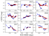 |
Fig. A.1. Combined light curve in the r band from the best solution in the third column of Table A.1. The A curve (red circles) is compared to the magnitude- and time-shifted B curve (blue squares). Open circles and squares are associated with the full brightness records, while filled circles and squares correspond to periods of overlap between both records. In the overlap periods, magnitudes of B are binned around dates of A using α = 20 d (filled squares; see main text). |
In Paper II, we also tried to account for all extrinsic variability using cubic splines and the PyCS software (Tewes et al. 2013; Bonvin et al. 2016). However, such a method did not produce very robust results because it was not originally designed to model extrinsic variations that are as fast as or faster than intrinsic ones (Tewes et al. 2013). Despite this fact, we obtained a 1σ confidence interval  d using simulated light curves and a weak prior on the true time delay (i.e. it cannot be shorter than 30 d or longer than 60 d). Hence, the spline-like microlensing model led to a significantly enlarged error bar, which is adopted in this paper. We think this 1σ interval is exaggeratedly large, and thus very conservative. First, considering only long-timescale extrinsic variability, a decade of monitoring observations with the LT and other telescopes strongly supports an error bar covering the delay range of 46−50 d (see above). This model exclusively has one non-linear parameter (time delay) and is appropriate. It accounts for extrinsic variations that distort the apparent long-term intrinsic signal, while the short-term extrinsic signal is assumed to be an extra-noise. Second, when all extrinsic variability is modelled, one deals with a complex non-linear optimisation, which may yield local minima, degeneracies, and so on. We have not yet found a fair way to simultaneously fit the delay and all microlensing activity. Despite these drawbacks, we are working on PyCS-based codes to account for the full microlensing signal in SDSS J1339+1310-like systems. These codes could produce robust results in a near future.
Best solutions for α = 20 d.
All Tables
All Figures
|
Fig. 1. Light curves of SDSS J1339+1310AB from its discovery to 2019. These r-band brightness records of the two quasar images are based on observations from four different facilities that are labelled as LT, MT, ST, and PS1 (see main text). Magnitudes of a field star are offset by +2.0 (triangles) to facilitate comparison with strong quasar variations. Dates of spectroscopic observations are marked by vertical dotted lines. |
| In the text | |
|
Fig. 2. HST-WFC3-UVIS spectra of SDSS J1339+1310AB in February 2016. The first order spectra are A+ and B+ (+1st order data), as well as A− and B− (−1st order data). Fluxes from LT r-band frames on 14 February 2016 are also shown for comparison purposes. |
| In the text | |
|
Fig. 3. VLT-X-shooter spectra of SDSS J1339+1310ABG in April 2017. The fluxes in the UVB, VIS, and NIR arms are depicted in the top, middle, and bottom panels, respectively. Grey highlighted regions display very noisy behaviours that are related to strong atmospheric absorption. |
| In the text | |
|
Fig. 4. Multi-component decomposition of the C IV line profile in SDSS J1339+1310A. The profile is decomposed into three Gaussian components: C IV broad + C IV narrow + He II complex. The grey rectangles highlight the two spectral regions that we used to remove a linear continuum under the emission line, and the vertical dotted lines correspond to the centres of the Gaussians. Top panel: GTC-OSIRIS-R500B data in May 2014, while bottom panel: HST-WFC3-UVIS data in February 2016. |
| In the text | |
|
Fig. 5. Multi-component decomposition of the Mg II and Hβ line profiles in SDSS J1339+1310A. The data correspond to VLT-X-shooter observations in April 2017. The original wavelength bins contain a very noisy signal (lighter blue), so a nine-point median filter is used to smooth original data (darker blue). In the top panel, after subtracting a power-law continuum, the residual signal is modelled as a sum of two contributions, i.e. Mg II broad emission (Gaussian curve around the vertical dotted line) and Fe II pseudo-continuum. There is no evidence of a Mg II narrow line or an additional very broad component. The continuum windows at 2195−2215 Å and 3020−3070 Å are highlighted using grey rectangles, and the Fe II pseudo-continuum is created from the Fe II template of Tsuzuki et al. (2006) convolved with a Gaussian function to account for the Doppler broadening of Fe II lines. Bottom panel: decomposition in the spectral region around the Hβ emission. The grey rectangle highlights one of the two windows that we used to remove a power-law continuum under emission lines (3790−3810 Å and 5080−5100 Å; Kuraszkiewicz et al. 2002). The residual signal is decomposed into four Gaussian components: Hβ broad + Hβ narrow + [O III] doublet, plus the Fe II contribution from two individual lines in the spectral range 4750−5100 Å (e.g. Kovačević et al. 2010). Vertical dotted lines show the centres of the four Gaussians. |
| In the text | |
|
Fig. 6. Image Br-band light curve from the LT shifted by the 47-d time delay and subtracted from the contemporaneous magnitude of image A, i.e. mA(t)−mB(t + 47 d) (equivalent to a ratio in flux units), leaving only variability that is not intrinsic to the source itself. Plotted in black are five good fits to the microlensing variability from our Monte Carlo routine. |
| In the text | |
|
Fig. 7. Distributions for the effective source velocity and mean microlens mass. Left panel: probability density for the effective velocity |
| In the text | |
|
Fig. 8. Accretion disc structure in SDSS J1339+1310. Left panel: probability density for the source size in Einstein units (⟨M*/M⊙⟩1/2 cm). The distribution levels off at ∼2 × 1014 cm since the pixel scale in our magnification patterns is 1.6 × 1014 cm. All solutions become equally likely below that size scale. Right panel: probability density for the half light radius of the continuum-emission region in SDSS J1339+1310 at λrest = 1930 Å assuming an inclination angle cos i = 0.5. The solid black curve was derived by convolving our probability density for ⟨M*⟩ (right panel of Fig. 7) with that of |
| In the text | |
|
Fig. A.1. Combined light curve in the r band from the best solution in the third column of Table A.1. The A curve (red circles) is compared to the magnitude- and time-shifted B curve (blue squares). Open circles and squares are associated with the full brightness records, while filled circles and squares correspond to periods of overlap between both records. In the overlap periods, magnitudes of B are binned around dates of A using α = 20 d (filled squares; see main text). |
| In the text | |
Current usage metrics show cumulative count of Article Views (full-text article views including HTML views, PDF and ePub downloads, according to the available data) and Abstracts Views on Vision4Press platform.
Data correspond to usage on the plateform after 2015. The current usage metrics is available 48-96 hours after online publication and is updated daily on week days.
Initial download of the metrics may take a while.