| Issue |
A&A
Volume 643, November 2020
|
|
|---|---|---|
| Article Number | A87 | |
| Number of page(s) | 20 | |
| Section | Planets and planetary systems | |
| DOI | https://doi.org/10.1051/0004-6361/202038311 | |
| Published online | 06 November 2020 | |
Migration jumps of planets in transition discs
1
Institut für Astronomie und Astrophysik, Universität Tübingen,
Auf der Morgenstelle 10,
72076
Tübingen, Germany
e-mail: thomas.rometsch@uni-tuebingen.de
2
Institute for Theoretical Astrophysics, Zentrum für Astronomie, Heidelberg University,
Albert Ueberle Str. 2,
69120
Heidelberg, Germany
Received:
29
April
2020
Accepted:
5
September
2020
Context. Transition discs form a special class of protoplanetary discs that are characterised by a deficiency of disc material close to the star. In a subgroup, inner holes in these discs can stretch out to a few tens of au while there is still mass accretion onto the central star observed at the same time.
Aims. We analyse the proposition that this type of wide transition disc is generated by the interaction of the disc with a system of embedded planets.
Methods. We performed two-dimensional hydrodynamics simulations of a flat disc. Different equations of state were used including locally isothermal models and more realistic cases that consider viscous heating, radiative cooling, and stellar heating. Two massive planets (with masses of between three and nine Jupiter masses) were embedded in the disc and their dynamical evolution due to disc–planet interaction was followed for over 100 000 yr. The simulations account for mass accretion onto the star and planets. We included models with parameters reminiscent of the system PDS 70. To assess the observability of features in our models we performed synthetic ALMA observations.
Results. For systems with a more massive inner planet, there are phases where both planets migrate outward engaged in a 2:1 mean motion resonance via the Masset-Snellgrove mechanism. In sufficiently massive discs, the resulting formation of a vortex and the interaction with it can trigger rapid outward migration of the outer planet where its distance can increase by tens of au in a few thousand years. After another few thousand years, the outer planet rapidly migrates back inwards into resonance with the inner planet. We call this emerging composite phenomenon a migration jump. Outward migration and the migration jumps are accompanied by a high mass accretion rate onto the star. The synthetic images reveal numerous substructures depending on the type of dynamical behaviour.
Conclusions. Our results suggest that the outward migration of two embedded planets is a prime candidate for the explanation of the observed high stellar mass accretion rate in wide transition discs. The models for PDS 70 indicate it is not currently undergoing a migration jump but might very well be in a phase of outward migration.
Key words: accretion, accretion disks / protoplanetary disks / planet–disk interactions / hydrodynamics / methods: numerical
© ESO 2020
1 Introduction
Observationally, transition discs are characterised by a lack of flux in the micrometre (near- to mid-infrared) range as seen in the spectral energy distributions (SEDs) of young stars. This flux deficit is typically associated with “missing” dust and with temperatures of 200–1000 K (Calvet et al. 2002; D’Alessio et al. 2005) corresponding to the inner regions of accretion discs. Despite this lack of dust, there are still signatures of gas accretion in several systems with large inner (dust) holes that are a few tens of astronomical units (au) in width (see e.g. Espaillat et al. 2014).
The observational properties of transitional discs (TDs) and previous modelling attempts have been reviewed by Owen (2016) and here we mention only the main aspects relevant to this paper. The origin of the inner disc clearing is primarily attributed to three different processes: photoevaporation from the inside out through high-energy radiation from the central young protostar (e.g. Shu et al. 1993; Alexander et al. 2006), magnetically driven disc winds (e.g. Rodenkirch et al. 2020), or embedded massive companions that carve deep gaps into the disc (e.g. Varnière et al. 2006). Additionally, TDs appear to come in two flavours, millimetre(mm)-faint discs with low mm fluxes, small inner holes (≲10au), and low accretion rates onto the stars (≈10−10−10−9 M⊙ yr−1), and mm-bright discs with large mm fluxes, large holes (≳20 au), and high accretion rates ≈10−8 M⊙ yr−1 (Owen & Clarke 2012) to which we refer here as Type I and Type II discs, respectively.
While photoevaporation is certainly at work in some systems (Type I TDs), it is believed that it can only operate for systems with a sufficiently low mass accretion rate below 10−8M⊙ yr−1 and is otherwise quenched by the accretion flow (Owen & Clarke 2012). At the same time the persistence of gas accretion within the inner (dust) holes is taken as an additional indication that other mechanisms should operate that create these gaps (Manara et al. 2014). The very likely mechanism for this second class of TDs is related to the growth of planets in the discs, because young planets embedded in their nascent discs will not only open a gap in the gas disc but will create an even stronger depletion of the dust near the planetary orbit (Paardekooper & Mellema 2004).
Consequently, it was suggested early on that the presence of a massive (Jupiter-sized) planet might be responsible for the gap creation (Varnière et al. 2006; Rice et al. 2006), but at the same time it has been reported that the gap created by a single embedded planet is significantly narrower than suggested by observations of transition discs. Given the problems with a single planet and the photoevaporation models, it has been proposed that the main observational features can be created by the presence of a system of (three to four) massive planets. Following this line of thought, Zhu et al. (2011) and Dodson-Robinson & Salyk (2011) performed numerical simulations and argue that TDs are in fact signposts of young multi-planet systems. In this scenario, the embedded planets act as a “barrier” for the gas flow through the disc, allowing some gas to enter the inner region, causing the observed accretional features near the star, while the dust is filtered out at the pressuremaximum just beyond the outer edge of the gap and cannot enter the inner disc regions. Following this line of thought, theoretical models with embedded planets and dust in discs have been constructed to match the observed spectral energy distributions at sub-millimetre wavelengths (de Juan Ovelar et al. 2013; Pinilla et al. 2015).
New ALMA observations focusing on CO-rotational lines have allowed the gas content to be determined in the inner disc region in more detail. These results show that the inner disc gas depleted by factors of about 102 (van der Marel et al. 2015), or even by a factor of 104 with gas holes about a factor 2–3 smaller than the dust gaps (van der Marel et al. 2016), which is taken as another example of massive planets in discs (Ho 2016). The conclusion that all or the majority of Type II TDs are shaped by massive planets was questioned by Dong & Dawson (2016) who argue that there may not be enough giant planets to explain all the observed Type II TDs; see also Cumming et al. (2008) for the occurrence rate of massive planets at larger separations. The solution to this problem is either that current numerical models of planet–disc interactions are too inefficient at gap opening compared to what is seen in nature, or that Type II TDs are intrinsically rare objects rather than being common and short-lived as is probably the case for their Type I counterparts. Considering that the arguments of Dong & Dawson (2016) are based on analytical approximations of gap widths and sizes that are based on isothermal disc models, it may well be that the theoretical models have not reached the degree of sophistication necessary to produce reliable results.
Recent evidence in favour of the planet-based origin of Type II TDs came through the direct detection of embedded planets in such systems. For the T Cha system, the presence of a planet was suggested based on observations in the L-band (Huélamo et al. 2011) which were later supported by ALMA observations indicating a gap in the disc ranging from 18 and 28 au compatible with a 1.2 MJup planet (Hendler et al. 2018). However, direct confirmation is still pending. A point-like source was detected in the L-band in the transition disc system MWC 758 at a deprojected distance of about 20 au from the star (Reggiani et al. 2018), directly hinting at the presence of an embedded planet. However, the clearest evidence comes from the PDS 70 system. A first point like object was detected in the near-infrared at a projected distance of 22 au, which was attributed to a planet (PDS 70b) orbiting within a gap that stretches from about 17–54 au in size (Keppler et al. 2018). The large gap size in PDS 70 suggested a second companion which was detected last year (Haffert et al. 2019). The authors confirmed the earlier Hα detection of PDS 70b and found a second point-like Hα source near the outer edge of the gap. This Hα emission is taken as evidence for ongoing accretion onto two proto-planets (Haffert et al. 2019). In addition, the spatial separation of the two planets indicates that they are close to a 2:1 mean motion resonance (MMR).
With respect to PDS 70, a few simulations of embedded planets have been performed. The first study (Muley et al. 2019) considered only one planet and a possible explanation of the wide gap was the creation of a large eccentric cavity by a massive planet of about 2.5 MJup. While this is in principle a possible scenario for sculpting transition discs, as shown also by Müller & Kley (2013), the direct observation of a second planet ruled out this scenario for PDS 70. Consequently, two-planet simulations were presented that show that a system engaged in a 2:1 MMR can in fact be stable for several million years (Bae et al. 2019).
In this paper we study the evolution of planets embedded in protoplanetary discs using two-dimensional hydrodynamical simulations. Our simulations include planet migration and mass accretion and either assume a locally isothermal equation of state or incorporate stellar heating and radiative cooling from the disc. This work extends an earlier study (Müller & Kley 2013) where only one planet was considered, which remained on a fixed orbit around the star and was not allowed to migrate through the disc. First, we present generic models to demonstrate our new findings on the occurrence of migration jumps. We then present our study of the system PDS 70. For both cases, we generate synthetic images and discuss the observability of the features.
In Sect. 2, we introduce our numerical model. In Sect. 3, we present the evolution of the planetary system in our numerical simulations and describe migration jumps in detail. In Sect. 4, we generate synthetic images of a disc in our simulations and identify possible observational features. Section 5 is a case study of how migration jumps apply to the PDS 70 system. We discuss our findings in Sect. 6 and give a summary in Sect. 7.
2 Modelling
In this section we describe the physical and numerical setup used in our simulations. To give an overview of the cases investigated, Table 1 lists all models and summarises their most important parameters. Specific models are referred to using a short label in sans serif font.
2.1 Physical setup
We model an accretion disc around a young protostar solving the two-dimensional (2D, r− ϕ) viscous hydrodynamical equations obtained by averaging over the vertical direction. Most of our models assume a locally isothermal equation of state (T = T(r) is constant over time). For selected models (IRR, PDS70 IRR, PDS70 IRR M/5) we solve the energy equation and include heating by irradiation from the star (analogous to Ziampras et al. 2020), viscous heating, and radiative cooling, using an averaged opacity. All the details of the used set of equations are stated in Müller & Kley (2012, 2013). Here, we do not solve for radiative transport within the plane of the disc.
For the systems investigated here, the locally isothermal assumption and the inclusion of the radiative effects yield comparable results as the test in Appendix B shows.
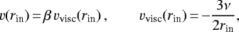
Viscosity is parameterised with the α viscosity model (Shakura & Sunyaev 1973) using a value α = 10−3. The kinematic viscosity is then ν = αcsH with the sound speed cs and the vertical pressure scale height of the disc H. Together with the choices for Σ and H∕r (as given below) this value of α corresponds to a viscous mass accretion rate Ṁdisc = 3πΣν = 5.3 × 10⁻⁹ M⊙ yr−1 at 2 au for the initial profile (see also panel 2 of Fig. 1).
The host star mass is M* = 1 M⊙. There are two planets embedded in the disc. The inner planet (1) is initially located at a1 = 4 aJup = 20.8 au with a mass of M1 = 3–9 MJup and the outer planet (2) is initially located at a2 = 7 aJup = 36.4 au with a mass of M2 = 1–9 MJup. These models are labelled with Mk-l where k/l is the mass of the inner/outer planet in MJup, respectively.The exact combinations of masses can be found in Table 1. For all combinations of planet masses, a large deep gap can be expected in the disc.
To simplify the simulations, self-gravity of the disc is neglected in most of them. For the initial conditions of our standard model M9-3 the Toomre Q parameter isabove 3 at 100 au and above 8 close to the location of the planet. Thus, self-gravity should not play a dominant role in the system considered. This assumption is verified by two additional models with self-gravity included. The corresponding models are described in Sect. 2.8.
Model parameters and outcome of the simulations.
2.2 Simulation code
The hydrodynamics equations are solved on a 2D polar grid (using r− ϕ coordinates). Radially, the domain ranges from 2.08–208 au covered by 602 cells that are logarithmically spaced. Azimuthally, the grid is uniformly spaced from 0 to 2π with 821 cells.
We use a custom version of the FARGO code (Masset 2000), which was also used by Müller & Kley (2013) in an earlier version, and is further developed and maintained by our group at the University of Tübingen. N-body calculations are performed with the IAS15 integrator in REBOUND (Rein & Liu 2012) which is integrated into our version of FARGO.
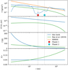 |
Fig. 1 Initial conditions for the disc around the 1 M⊙ star used in our simulations (blue). These are compared to the initial conditions of the disc in Bae et al. (2019) (green) in which the PDS70 system (0.85 M⊙ star) was modelled. For context, the surface density of the minimum mass solar nebula (MMSN; Hayashi 1981) is plotted in orange. Physical initial conditions after the equilibration phase (see Fig. 2) at t = 26 kyr are shown for model M9-3 as a dashed blue line. The panels, from top to bottom, show the radial profile of the: surface density, viscous mass accretion rate (Ṁdisc = 3πΣν with α = 10−3), temperature, and aspect ratio. The initial location of the planets are marked by the vertical, dotted lines which span over all panels and are indicated by the red and cyan circles. |
2.3 Initial conditions
Initially, the surface density of the disc Σ is set to a power-law profile of the form
 (1)
(1)
The aspect ratio of the disc is chosen as  throughout the disc, which is equivalent to choosing a temperature power law of
 (2)
(2)
We checked this assumption by performing additional simulations using irradiated discs; see Appendix B.
Both initial conditions are visualised in Fig. 1. The top panel shows Σ(r). The second panel from the top shows the viscous mass accretion rate, Ṁdisc = 3πΣν, at each radius in the disc assuming α = 10−3. The panel below that, and the bottom panel, show T(r) and the resulting disc aspect ratio, H∕r, respectively. To establish a context, we also show the initial conditions of a PDS 70 simulation by Bae et al. (2019, hereafter B19) and the minimum mass solar nebula (MMSN; Hayashi 1981). Our disc has a lower Σ than the MMSN in the inner ≈ 60 au and is about five times larger than the Σ in B19, who model the 5.4 Myr old PDS 70 system with a 0.85 M⊙ star. Their disc is lighter, as might be expected for an older system due to disc dispersal, and has lower temperatures in the inner parts of the disc due to lower stellar luminosity. The first panel also displays Σ(r) after the initial equilibration phase as the dashed blue line. The locations of the planets are marked by the dotted vertical lines and the red and cyan circles in the top panel.
These power-law initial conditions do not take into account the presence of embedded planets. To obtain more physical initial conditions which are consistent with two massive embedded planets, we insert the planets by ramping up their masses over 0.5 kyr while they are fixed at their orbits for an initialequilibration time, Teq. During this time, the N-body system evolves without being subjected to the gravitational force of the disc while the disc is exposed to the forces of the N-body system and a common gap forms around the planets. To determine Teq, we analysed test simulations and checked for the time when the density waves caused by the insertion of the planets left the computational domain and the time after which the gap depth no longer changed significantly. The second condition is fulfilled at a later time and yields Teq = 26 kyr which corresponds to 274 orbits at the initial location of the inner planet. After this time, the disc feedback onto star and planets is turned onwhich causes them to migrate. The equilibration process is sketched by the flow chart in Fig. 2.
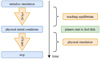 |
Fig. 2 Flow chart illustrating the equilibration and simulation phase. The disc properties are initialised according to the power laws in Eqs. (1) and (2). During the equilibration process (taking 26 kyr, equivalent to 274 orbits at the initial location of the inner planet) where the disc begins to “feel” the planets, the density profile changes significantly; see the first panel of Fig. 1 for the difference, where the equilibrated profile is shown as the dashed blue line. |
2.4 Boundary conditions
We employ an outflow boundary (O) condition at both radial boundaries, Rmin and Rmax. This is doneto let the disc evolve on its own, for example by allowing for an eccentric disc close to the inner boundary which might be unphysically suppressed by the use of a wave damping boundary, for example, that imposes an azimuthal symmetry close to the boundary. Additionally, this choice of boundary condition allows density waves that are created by the insertion of the planets to leave the computational domain.
For our outflow boundary condition, only mass flow leaving the domain is allowed. This is implemented by enforcing a vanishing gradient of the energy density and Σ, and by setting the radial velocity to zero at the boundary in cases where the velocity vector points into the domain and by setting its gradient to zero otherwise. This way, no mass can be generated. The azimuthal velocity is left unchanged.
In order to check the validity of these boundary conditions for our physical setup, we studied other options. This is important because the open boundary condition leads to an unphysical drop in surface density close to the boundary, as can be seen in the top panel of Fig. 1.
One alternative is to employ an additional wave damping (WD) zone (de Val-Borro et al. 2006) between Rmin and 2 Rmin where Σ and the velocities are exponentially damped to their initial values on a timescale of 5% of the orbital timescale at Rmin (models WD at half resolution). We combine this wave damping zone with the outflow boundary and with another common choice: a closed, reflective boundary. This reflective boundary does not allow mass flow through the boundary which is implemented by applying a zero gradient for energy density and Σ, and by setting the radial velocities of the ghost cells to zero at the boundary and to the negative of the first active cell’s radial velocity at the next ghost cell interface, thus reflecting momentum at the boundary. A combination of a reflective boundary and a wave damping zone is used in model WDR.
An outflow boundary as used in our simulations might overestimate the mass flow across the inner domain. In a real system, the properties of the accretion process onto the star are likely to limit the mass flow at the inner disc edge. To test for the implication of this, we also employed a viscous internal boundary. For this, the velocities of the inner ghost cells are set to a multiple of the viscous speed:
 (3)
(3)
with ν being kinematic viscosity. We used β = 1 (model VB) and β = 5 (model VB5) which was found to yield a boundary comparable to simulations where the 2D grid is embedded in a larger 1D domain (Crida et al. 2007). This boundary is also used to compare to similar models in the literature (e.g. Marzari et al. 2019).
2.5 Centre-of-mass frame
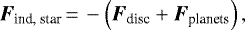
Many simulations of planet–disc interactions use a grid centred on the primary star. If there is only one gravitating object, this is an inertial frame. However, with the addition of one or more planets, it is not an inertial system any more and the so-called indirect term, which is the negative of the force acting on the star,
 (4)
(4)
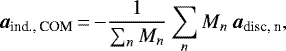
has to be applied to the bodies and the gas. For more massive planets, this causes the disc to oscillate for as much as the star oscillates around the centre of mass, which is undesirable from a numerical point of view. For a full planetary system, we obtain an inertial system by choosing the centre of mass of the N-body system as the origin. The indirect term therefore vanishes except for the contribution from the disc, which reads
 (5)
(5)
for all N-body objects indexed by n with mass Mn. To avoid any numerical drift of the centre of mass away from the origin, we shift the whole N-body system at every hydrodynamical time-step such that the centre of mass coincides with the origin, see also Thun & Kley (2018).
2.6 Gravitational interactions
Star and planets are modelled as point masses. The gravitational pull from the point masses onto the disc is implemented via their gravitational potential, which is
 (6)
(6)
at location r, and the index n runs over all point masses with masses Mn and position vectors rn. The smoothing length is chosen to be ɛsm = 0.6H(r), with the local disc scale height H(r), to approximate the gravitational force in a 3D disc (Müller et al. 2012).
The back reaction from the disc onto the point masses is calculated by direct summation over all grid cells, which are indexed by k, and have masses mk and positions rk. The total disc force acting on a point mass with index n is
 (7)
(7)
where ɛsm is the same as used for the potential.
2.7 Implementation of planetary accretion
In some simulations we include the possibility of mass accretion onto the embedded planets. We use the prescription from Dürmann & Kley (2017) and remove a fraction of mass every time-step Δt from the hydrodynamical simulation in the vicinity of the planet. More mass is removed from close to the planet than from further away. No mass is removed beyond a distance of 0.5 RHill from the planet’s location. For full details see Dürmann & Kley (2017). The mass removed at each time-step follows the relation
 (8)
(8)
where facc is a free parameter to control the efficiency of the accretion process. We use values of facc = 10−4, 10−3, 10−2 and 10−1 (models Afacc with facc in decimal notation). Mass and angular momentum are conserved by adding the mass removed from the hydrodynamical simulation to the mass of the planet and adding an equivalent amount of angular momentum.
2.8 Additional models
In order to test our model choices, we ran additional simulations with different parameters.
To check the impact of a constant aspect ratio, we reran the standard model M9-3 with a flaring aspect ratio of  (model FLARE). This flaring corresponds to a disc dominated by irradiation and h = 0.05 is reached at 30 au.
A resolution test was carried out by reducing or increasing the resolution by a factor of two ( in each direction, models M9-3 HR and M9-3 DR). See Appendix A for the comparison. To test the influence of the domain size, half resolution models (same Δr∕r as M9-3 HR) were done with a larger grid spanning from 5.2 to 520.0 au (models L, L M/2, L M/10). For the larger domain, density waves which are caused by the insertion of planets take longer to leave the domain. Therefore, Teq = 59 kyr is chosen.
Some models were run with a lower surface density but otherwise identical parameters to their sibling models. These are indicated by the M/N in their label and were initialised with N times smaller surface density compared to Eq. (2) (models M9-3 M/10, L M/2, L M/10 and PDS70 IRR M/5).
To test the effect of the centre of mass frame, we repeated some models with a coordinate system centred on the primary star. These are indicated by a -P in their labels (models VB-P, VB5-P, WD-P, WDR-P).
Most of our models do not include self-gravity. To test the implications of self-gravity, we ran two additional models with self-gravity included. This was implemented in the same way as in Baruteau (2008), but with a modified smoothing length that includes a dependence on radius in order to fulfil Newton’s third law (Moldenhauer & Kley, in prep.). The two models are based on model VB5-P for runtime reasons because this model has the largest time-step. Model SG has only self-gravity enabled and SG IRR additionally solves the energy equation and considers irradiation like model IRR.
We also ran a set of models to simulate the PDS 70 system. The parameters and results are discussed separately in Sect. 5.
3 Results
In this section, we analyse the simulations listed in Table 1 with respect to their dynamical evolution and accretion properties. Each effect is described in a separate subsection.
Due to the large number of simulations performed, we do not visualise all of them. Instead, we used a representative selection to highlight the various dynamical evolutions. Unless stated otherwise, the features observed in those simulations that are not displayed are very similar but might happen at a different point in time.
The simulation outcomes are described in the following sections and an overview can be found in Table 1. The different properties listed are: outward and inward migration (↗ and ↘, Sect. 3.1), migration jumps (indicated by ✓, Sect. 3.2), single/double orbit swaps (S/DS, Sect. 3.3), and planet ejections (E, Sect. 3.6). Table 1 also refers to the corresponding figures, which show the migration history of the respective simulations.
3.1 Direction of migration
In all simulations, the planets start to migrate after gravitational feedback from the disc onto the planets is turned on. A selection of migrationtracks for simulations with different planetary masses and mass ratios is shown in Fig. 3. The selection showcases the different possible behaviours of the systems.
For all combinations of planetary masses, the inner planet is migrating outward for the first 10 kyr because it only feels the positive torque contribution from the inner disc. There is no substantial contribution to the torque from the outer disc because of the large common gap opened by the two planets. Regions where the interaction of the disc would be strongest (Ward 1997) are cleared by the outer planet (Sándor et al. 2007). Vice versa, the outer planet migrates inward for the first 10 kyr. After this time, the planets are captured in a 2:1 MMR. We verified this by checking the resonant angles for an inner MMR,  (Forgács-Dajka et al. 2018), where λ = M + ϖ is the mean orbital longitude with the mean anomaly, M, and ϖ = ω + Ω is the longitude of periapsis with the argument of periapsis, ω, and the longitude of the ascending node, Ω. These angles are indeed librating around zero (see Fig. 4 where
  are displayed). Being locked in resonance, the planets then migrate in unison with a direction that depends on whether the positive torque contribution of the inner disc (inside the common gap) is larger in magnitude than the negative torque contribution from the outer disc (outside the common gap). As these torque contributions depend on the respective planetary mass, the direction of migration can vary. If the inner planet is more massive than the outer planet, the system can migrate outwards as found initially for the Jupiter–Saturn system by Masset & Snellgrove (2001). Indeed, Fig. 3 shows outward migration for the M9-3 and M9-4.5 models for which the inner planet is more massive than the outer one. Conversely, the planets migrate inward for a more massive outer planet as in model M3-9. For equal-mass planets (M6-6), the system still migrates inward, but with a lower migration rate.
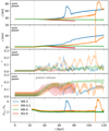 |
Fig. 3 Migration history for a selection of models described in Table 1 to highlight the different possible dynamical evolution of the embedded planets. The panels show, from top to bottom, the evolution of: the semi-major axis, a, of the outer and inner planet, their eccentricities, e, and their period ratio. The release time of the planets is marked by the vertical dotted line. Most prominent is the occurrence of fast outward migration (migration jump) for model M9-3 (blue) between 60 and 80 kyr, and a double orbit swap at 110 kyr followed by a migration jump for model M9-4.5. At the time of the double orbit swap at t ~ 110 kyr, ein = 0.38 and eout = 0.58. They are cut out to increase the visibility of the rest of the data. |
3.2 Migration jumps
Simulations in which the planet pair shows outward migration occasionally exhibit an additional process, which we call a “migration jump”:
- 1.
the outer planet embarks on a rapid outward migration covering tens of au in a time period of a few thousand years;
- 2.
after reaching a maximum radius, it stays in this region for several thousand years, occasionally for up to tens of thousands of years;
- 3.
it migrates back inward, again on a short timescale, until it locks back into resonance with the inner planet.
Two examples of a migration jump can be seen in Fig. 3. This process can repeat itself multiple times (see Fig. B.1).
Figure 4 shows a zoom into one migration jump of our standard M9-3 model focussed on the time leading up to the event and some time afterwards. It shows from top to bottom: the semi-major axis of both planets, their eccentricities, the 2:1 MMR angles, and the 4:1 MMR angles. The MMR angle variables correspond to an inner MMR (Forgács-Dajka et al. 2018). The two-dimensional surface density distribution of model M9-3 is displayed in Fig. 5, where panels a–f show the disc prior, during, and after the migration jump. The times of the individual snapshots are indicated in Fig. 4 by the vertical lines. Panel a of Fig. 5 shows the disc at that point in time when disc feedback is turned on and the planets are allowed to migrate.
In the following paragraphs we examine the migration jump process more closely by analysing the behaviour around the time of each of the six snapshots of model M9-3.
- a)
Prior to the migration jump, both planets migrate outward in 2:1 MMR. During this time, the eccentricity of the inner planet, ein, grows up to 0.15, while the eccentricity of the outer planet, eout, fluctuates up to 0.125. The increase in eccentricity comes from the interaction of the planets with the vortex that is formed outside the common gap. Faint spiral arms are visible in the common gap during this epoch (see panel b in Fig. 5).
- b)
At 64 kyr, ein drops significantly while eout rises up to 0.2 and the 2:1 MMR is broken. Due to its eccentric orbit, the outer planet comes close to the inner edge of the outer disc (see panel b of Fig. 5). This is close enough to sufficiently enhance the mass flow across the planet’s orbit and produce co-orbital torques. These torques are positive, because gas with higher angular momentum flows inwards where it has a lower angular momentum. The difference in angular momentum is deposited onto the planet causing a positive torque. What follows is a phase of type III rapid outward migration (Pepliński et al. 2008) and the outer planet moves out from 40 au at 65 kyr to 72 au at 70 kyr, covering 32 au in only 5 kyr. More complex structures can be seen in the disc (see panel c in Fig. 5) which are the result of overlapping spiral arms and the outer planet opening a gap. During this time eout relaxes backto low values.
- c)
The fast outward migration stops at the location of the 4:1 MMR with the inner planet (see the third panel from the top in Fig. 4 where the resonant angles
 are displayed). The two planets remain in the 4:1 MMR for about 4 kyr at t ~ 70 kyr, where the outer planet remains around 75 au.
 - d)
Afterwards the 4:1 resonance is broken and the outer planet migrates back inward by 22 au within 3.5 kyr.
- e)
It ends up back in 2:1 MMR with the inner planet. The inner planet migrates outwards during the jump since the positive torque from the inner disc is dominating over the negative contribution from the outside which is weakened due to the common gap.
Migration jumps occur in a variety of models but details such as the distance or duration of specific sub-processes vary from model to model. The location where the jump stops is not necessarily at the 4:1 period commensurability for all simulations, as can be seen for example in Fig. B.1 which also shows period ratios close to 4.5 and 5. In general, the location can be expected to be determined by the interplay of N-body dynamics (the resonances), gas dynamics, and the rearrangement of gas density around the outer planet. Migration jumps only happen in the models in which: migration is directed outward, a vortex forms outside the common gap, and the disc mass is sufficiently high.
From these observations we can decipher two criteria that must be met for migration jumps to occur. First, the planet mass ratio must be such that the pair of planets migrates outwards. This can be the case when the inner planet is more massive than the outer one. Second, the disc mass needs to be high enough to facilitate sufficiently fast outward migration. This migration speed is needed to allow for the formation of a significantly massive vortex which in turn leads to large eccentricities of the outer planet. These large eccentricities are needed for type III rapid outward migration to be triggered. For insufficiently high disc masses, the system only migrates outward smoothly and no vortex forms (see also the low-disc-mass results for model PDS70 IRR M/5, Fig. 11).
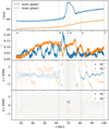 |
Fig. 4 Zoom-in on a migration jump in model M9-3 including the time leading up to and following the event. The panels show, from top to bottom, the evolution of: the semi-major axis of both planets, their eccentricities, the 2:1 MMR angles,
|

3.3 Orbit swaps
In addition to migration jumps, some models show other features as well. For example, the planets in model M9-4.5 swap their orbits in close succession just before a migration jump (Fig. 3 at 110 kyr). The orbital eccentricities reach very high values during the swapping process, for example eout = 0.58 in model M9-4.5. The accreting model, A0.01, also experiences a double swap (Fig. 7 at 90 kyr). A model with different resolution, model L, shows a single orbit swap (see Fig. 9). As a consequence, the inner planet is less massive than the outer one and the migration direction changes from outward to inward. Just after the single orbit swap, the outer, more massive planet undergoes a small migration jump (5 au). The models with self-gravity enabled also show orbit swaps. Model SG shows a single orbit swap following two migration jumps and model SG IRR shows a migration jump followed by a double orbit swap and a subsequent single orbit swap. In each of our non-self-gravitating simulations where an orbit swap (single or double) happens, a migration jump follows after a few more orbits. Events like orbit swaps have already been observed in the literature, especially in planetary systems with more than two massive planets (e.g. Marzari et al. 2010; Zhu et al. 2011).
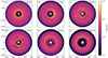 |
Fig. 5 Snapshots of the surface density for model M9-3 showing the disc at different times: prior (panels a and b), during (c and d), and after (e and f) a migration jump. The current orbits of the two planets are marked by the dotted white ellipses and the planetary Hill spheres are indicated by the small circles. Coordinate labels show the position in au. The snapshots are rotated to have the outer planet fixed on the horizontal axis to the right of the origin. Time inside the simulation is shown in the upper right corner. The time of a particular snapshot in the time-line of the simulation can be located on the annotated vertical lines in Fig. 4. For synthetic observations of the snapshots, see Fig. 10. |
3.4 Vortex outside the gap
During the regular outward migration of the planet pair, an overdensity is formed just outside the common gap, which is visible as the banana-shaped high-density structure just beyond the outer planet in panel b of Fig. 5. This is a sign of vortex formation by embedded planets in discs, which are known to occur for massive planets and/or low viscosity discs (e.g. Koller et al. 2003; Ataiee et al. 2013). Figure 6 shows a zoomed-in view of the overdensity and shows the surface density and streamlines in a system corotating with the overdensity. The eye of the vortex is visible in the upper right quadrant. Vortensity and surface density are analysed in more detail in Appendix C, where it is confirmed that the overdensity is indeed a vortex. In all our simulations in which a migration jump happened we also observed a vortex forming outside the common gap.
 |
Fig. 6 Zoom-in on panel b of Fig. 5 showing the surface density and velocity streamlines. The streamlines are computed in a frame corotating with the disc at 59 au. The streamlines are closed in the region indicated by the black arrow, showing that the overdensity is a vortex. The orbits of the planets are indicated as the green dotted lines. |
3.5 Accretion onto the star and planets
3.5.1 Planetary accretion
The accretion rates onto the planets and the star are shown alongside the dynamical evolution of the system in Fig. 7. Mass accretion onto the planets is turned on when the planets are released. The accretion rates onto the inner planet and the outer planet, Ṁin/out, scale approximately linearly with facc, as one might expect (see Eq. (8)). This behaviour holds during the inward migration of the outer planet into 2:1 MMR and during outward migration of the pair as long as the eccentricity of the outer planet remains below eout = 0.1. Due to the larger relative size of the inner planet’s Hill sphere (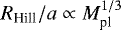 ) and its smaller orbital period, Ṁin is larger than Ṁout. This is because the mass available for accretion onto the inner planet is supplied via the streamers within the common gap. The accretion rate is then determined by the ratio between a planet’s region of influence (RHill) and the length of its orbit (a), that is, by how much of the mass around its orbit is accessible to it, and by its orbital frequency, in other words, how often it encounters these streamers. The larger accretion rate of the inner planet also shows that the outer planet only receives a small fraction of the gas that otherwise travels through the common gap and does not starve the accretion of the inner planet. During these quieter times, the models behave very similarly, and independently of facc, although the facc = 0.1 case shows the same events at a slightly earlier time.
Around t = 47 kyr (first vertical dashed line in Fig. 7) when eout rises to values above 0.1, Ṁin/out increases as well. This can be explained by the following argument. When the outer planet comes close to the outer gap edge at apastron, it “shovels” disc material inwards into the common gap (see panel b in Fig. 5 for the emerging structures). Thus, there is more gas available inside the planets’ Hill spheres to be accreted. This way, outward migration with pumping of eccentricities can enhance planetary accretion. Variabilities of Ṁin/out occur on timescales of around two times the period of the outer orbit. Ṁin follows the same trends as Ṁout with a delay of around one outer period (~200 yr) because of the finite gap-crossing time.
At around t = 50 kyr (second vertical dashed line in Fig. 7), Ṁin/out reach their highest values prior to the migration jumps before they decrease when eout relaxes to lower values. During the smooth phase of outward migration, Ṁin/out can be increased by a factor of 10–20 compared to inward migration.
Just before the onset of a migration jump (third vertical dashed line in Fig. 7), eout and Ṁin/out rise again. Models A0.0001, A0.001, and A0.1 show a migration jump soon after, at around t ~ 66 kyr. During the jump (fourth vertical dashed line in Fig. 7), Ṁout is comparable to Ṁin because the outer planet moves through the disc and has a higher density of gas inside its Hill sphere. Ṁin also rises as significant amounts of gas are scattered inward during the jump. This can result in a 50–100 fold increase compared to the values during inward migration.
A notable exception to the described behaviour is model A0.01. There, the first migration jump fails, which gives rise to another distinct behaviour. Similar to the other models, the outer planet increases the mass flow through the gap by “shovelling” gas into it. However, unlike the other models, it does not embark on a jump and continues to supply material to the inner planet. This causes the gas density of the inner planets Hill sphere to rise and Ṁin to rise tenfold, matching the rates of the A0.1 model. At t = 91.7 kyr (fifth vertical dashed line in Fig. 7), Ṁout on A0.01 also matches the values of A0.1, where it finally embarks on a jump and its eccentricity has risen to eout = 0.2.
Figure 8 shows the time evolution of the mass accreted onto the planets and the star and the total disk mass. Depending on the efficiency of planetary accretion, facc, the changes in planet mass can be substantial, as seen in the first two panels. The most extreme case is the outer planet of model A0.1 which has almost doubled its mass at the end of the simulation.
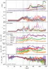 |
Fig. 7 Evolution of accretion rates, migration, and eccentricities for the models with planetary accretion.Then panels show from top to bottom: the semi-major axis of both planets, ain/out, the eccentricity of the inner planet and that of the outer planet, ein/out, planetary mass accretion rate onto the inner and outer planet, Ṁin/out, and the mass accretion rate onto the star smoothed with a moving average of length 1.185 kyr, Ṁ*. The vertical dashed lines indicate events of interest and are referred to in Sect. 3.5. Model A0.0 is an alias for model M9-3. |
3.5.2 Stellar accretion
Mass accretion onto the star, Ṁ*, is calculated by summing the mass that leaves the inner boundary over the output interval of 11.8 yr. It does not show a dependence on the efficiency of planetary accretion, facc. The mass lost through the inner boundary is not added to the primary star because its contribution to the total stellar mass over the time-span of the simulations would be smaller than 1% (see third panel of Fig. 8) and can be neglected. For a theoretical estimate of the stellar mass accretion rate we can use the viscous mass accretion rate of the unperturbed disc at the inner boundary (≈2 au) which is Ṁdisc = 3πΣν = 5.3 × 10⁻⁹ M⊙ yr−1. In the simulations, the mass accretion rates onto the star through the inner boundary fluctuate between 10−8 and 10−7 M⊙ yr−1. One should keep in mind that the theoretical estimate does not take into account the presence of the massive embedded planets, which can be expected to substantially alter the dynamics of the disc. This discrepancy could be explained by the inner outflow boundary and changes in the disc structure. Because there is no pressure support from the inside, there is a high mass flow in the radial direction. An additional contribution arises when the disc becomes eccentric in its inner region. The simulations show gas eccentricities between 0.1 and 0.4 in the inner 10 au of the domain, which are a result of the gravitational interaction of the planets and the disc. Since the boundary is perfectly circular by design, any gas that is on an eccentric orbit which overlaps with the boundary is lost through the boundary because it cannot reenter, although its orbit would bring it back into the domain. Therefore, the accretion rate onto the star, Ṁ*, can only be seenas an upper limit.
Models VB-P and VB5-P, which employ a viscous boundary to avoid abnormally high mass flow through the inner boundary, show mass accretion rates at a similar level, with values around Ṁ* ~ 2 × 10⁻⁸ M⊙ yr−1 for both choices of vin (β = 1 or 5 in Eq. (3)). This means, that the surface density of the inner disc must be enhanced compared to the initial condition, which is indeed the case for simulations showing outward migration. This result can be taken as an indication that the outflow boundary in our simulations does not strongly overestimate the mass accretion through the inner boundary. On the contrary, in our simulations, the stellar accretion rate seems to be determined by the amount of gas that can be supplied from further out in the disc.
A special behaviour was observed in model L which exhibits a single orbit swap, as explained in Sect. 3.3. Because migration changes from outward to inward in an otherwise unchanged disc, this model gives us the opportunity to study how Ṁ* depends on the direction of migrationand the ordering of the planets. Figure 9 shows migration and eccentricities of both planets (top and middle panel) and Ṁ* smoothed with a moving average of length 1.185 kyr (bottom panel) for model L. The small Ṁ* at t = 100 kyr is due to the initialisation phase when the inner disc is mostly depleted by accretion through the inner boundary. In the time after planet release, the inner disc recovers parts of its mass and reaches up to a tenth of its initial value of Σ at t = 150 kyr and a fourth at t = 250 kyr by mass transfer through the gap. This is enough to start outward migration. In the 120 kyr of outward migration leading up to the migration jump, accretion is enhanced to Ṁ*≈ 2 × 10⁻⁸ M⊙ yr−1 (see bottom panel of Fig. 9). After the planets swap orbits at 300 kyr, migration changes its direction to inward and accretion deceases to values Ṁ* < 10−9 M⊙ yr−1. The eccentricity of the massive planet and the value of Ṁ* follow similar trends (see Fig. 9). However, both values are not proportional which can be seen by comparing the values at 200 and 520 kyr where the eccentricity of the massive planet is at a value of 0.1, but Ṁ* is at least ten times smaller at the later time. This rules out the possibility that the increase in Ṁ* during outward migration is a result of the outflow boundary effect explained in the last paragraph. During the event of the orbit swap, there is no abnormally high mass loss of the disc. The disc mass in the whole domain only changes from 0.145 to 0.14 M⊙ after the planets are released, and so the change in Ṁ* cannot be explained by the disc suddenly loosing most of its mass. Thus, Ṁ* depends on the direction of migration and it is enhanced for outward-directed migration. The model also shows that mass can be transported through a common planet gap at a substantial rate. Summarising the results, we can report the following findings:
- 1.
Mass accretion through the disc can be sustained even in the presence of a large common gap carved by a pair of massive planets.
- 2.
Planetary accretion can be substantially increased when a pair of planets is migrating outward in 2:1 MMR where the increase in mass accretion can be 10–20 fold compared to inward migration.
- 3.
During extreme events like a migration jump, when a planet travels through previously unperturbed disc regions, the increase can be even higher with values increased 50–100 fold compared to inward migration.
- 4.
Migration rates seem not to be affected by the choice of facc during times of smooth outward migration. However, the accretion efficiency can change the type of occurring events and the timing when they happen.
- 5.
Mass accretion rates onto the star seem not to be affected by the choice of facc.
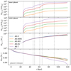 |
Fig. 8 Evolution of the mass accreted onto the planets and the star and the disk mass for the models with planetary accretion. The panels show from top to bottom: the mass accreted onto the inner and outer planet, Macc,pl, the mass which leaves the disc through the inner domain, Macc, *, (i.e. the mass that would be accreted onto the star, but which is not added to it in the simulations), and the evolution of the total disc mass, Mdisc. The evolution of Mdisk also includes the mass leaving the outer domain. The values are in units of the initial mass of the respective object for the accreted masses and in stellar masses for the disc mass. The dashed vertical lines correspond to the ones in Fig. 7. |
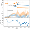 |
Fig. 9 Migration and accretion for model L showing the orbit swap and how Ṁ* depends on the direction of migration. The panels show (top) semi-major axis, a, (middle) eccentricity, e, and (bottom) migration onto the star Ṁ*. The verticaldashed line indicates the time when planets are allowed to migrate. |
3.6 Planet ejection
In some models, the planetary system is ejected either during a first or second migration jump. The outer planet is ejected first and the inner planet is ejected 2–3 kyr later. The models affected are VB, VB5, WD, and WDR. All of them use a disc (hydrodynamical simulation) centred around the centre of mass of the star and the two planets and have an inner boundary condition different from outflow. The affected inner boundary conditions are the viscous boundary with vin = vvisc and vin = 5vvisc, the outflowboundary with an additional wave-damping zone, and the reflective boundary with an additional wave-damping zone. We repeated all the affected models with the disc (hydrodynamical simulation) centred on the primary star (models VB-P, VB5-P, WD-P, and WDR-P). In the primary frame, no ejection occurred during the simulation time which was chosen to be at least 50 kyr longer than the time when the ejection happened in the corresponding centre-of-mass model.
In all the models, the inner boundary is located at 2.08 au and the wave damping zone stretches from the inner boundary to 4.16 au. This comparison shows that the inner boundary can be crucial for determining the fate of an embedded planetary system, even if planets are further out at around 50 au.
All ejection occurred in models where the primary star was moving with respect to the boundary. In the centre-of-mass frame, the primary moves up to 0.4 au, which is 20% of the inner boundary radius. This equivalently means that the boundary is moving 0.4 au relative to the star.
The difference is not only a numerical artefact, but the physical boundary condition is different for the models in the centre-of-mass frame compared to the primary frame. Using the viscous boundary condition in the primary frame for example, the radial speedat a fixed radius from the star is set to the viscous speed. This is a physically motivated choice. Since the hydrodynamical grid is centred on the primary, this boundary condition can be implemented in a simple way by setting the velocity at the inner boundary, which is at a constant distance from the star in all directions. Using the same implementation in a centre-of-mass frame, as we did in our models, the distance at which the radial velocity is set to the viscous speed is different depending on the azimuthal direction and is even varying over time. Thus, the resulting boundary condition is physically different from the case of the primary frame and is no longer physically plausible.
In all cases, except the zero-gradient boundary condition case, the unphysical boundary condition leads to strong perturbations close to the inner boundary, which at some point in time can no longer be resolved by the hydrodynamical simulations. In the resulting numerical instability, the perturbations grow unbound and destroy the disc and coincidently also eject the planets without any close encounter or instability in the N-body system.
3.7 Final location of outward migration
Most models were run for a simulation time of 120 kyr. At this point in time, outward migration did not halt in any of the models. Some models were integrated for a longer time, such as for example the M9-3 model in which the outer planet reached 133 au at t = 226 kyr. In this specific case, the outer gap edge is located at 162 au and the surface density of the outer disc is two orders of magnitude lower than that of the inner disc. As a result, the negative torque contribution from the outer disc becomes diminished and outward migration continues. Our models suggest that, in the scenario studied here, in the case of outward migration of a pair of planets in a disc of sufficiently high mass, the final location of the planet pair will be near the outer edge of the disc.
4 Observability
To evaluate the possibility whether or not the effects of migration jumps could be observed in real systems we performed synthetic observations. Though the timescale of the processes discussed here is quite short, some tens of thousands of years if we also include the time the structural changes last in the disc (see panels e and f of Figs. 5 and 10), the synthetic observations might be applicable to systems in which we directly observe embedded planets, such as PDS 70. These observations are, after all, just snapshots in time of the real system. With a disc lifetime of the order of roughly 1 Myr, the migration jump timescale of 10 kyr amounts to a significant fraction, that is, in the region of 1%. Considering the ever-increasing number of detected (proto-)planetary systems and the apparent richness in substructure therein (Andrews et al. 2018), the following synthetic images might provide an explanation for a subset of future disc observations. Our synthetic images were produced by calculating the thermal emission using RADMC3D (Dullemond et al. 2012). This emission was then postprocessed using the CASA package (McMullin et al. 2007) to simulate the instrumental effects produced by ALMA. The resulting synthetic observations of the M9-3 model are shown in Fig. 10 and can be directly compared to the plots of surface density in Fig. 5. The simulation snapshots are the same in the respective panels.
4.1 Radiative transfer model
In order to compute the thermal dust emission for the individual snapshots of the M9-3 model we convert the gas surface density profiles into a three-dimensional dust density model which serves as input for the radiative transfer calculations with RADMC3D. Please keep in mind that, in principle, dust follows its own dynamics and is only partially coupled to the gas. Our synthetic images are therefore only an approximation of what would be the result of the actual dust distribution taking into account the proper gas–dust interaction. In the model we employ eight dust species with a combined dust to gas mass ratio of 10−2. The dust grain sizes are logarithmically evenly spaced, ranging from 0.1 μm to 1 mm. The number density size distribution of the dust grains follows the MRN distribution n(a) ∝ a−3.5, where a is the grain size.
Dust settling towards the midplane is considered following the diffusion model of Dubrulle et al. (1995) with dust vertical scale height:
 (9)
(9)
where St is the local Stokes number,
 (10)
(10)
where the grain density ρd = 3.0 g cm−3. We assume a Schmidt number of one. Furthermore, the aspect ratio is assumed to be flared with radius, that is, H∕r scales as  where γ is the flaring index. In all the synthetic images, a flaring index of γ = 0.25 was chosen.
For the extension in the polar direction, 32 cells are equally spaced in their angular extent between θlim = π∕2 ± 0.3 resulting in a maximal spacial extent of zlim = r sin(±0.3). The vertical disc density profile is assumed to be isothermal and the conversion from the surface density to the local volume density is calculated as follows:
![\begin{align*} \rho_{\mathrm{cell}}\,{=}\,\frac{\Sigma}{\sqrt{2\pi} H_{\mathrm{d}}} & \cdot \mathrm{erf}^{-1} \left(\frac{z_{\mathrm{lim}}}{\sqrt{2} H_{\mathrm{d}}} \right) \\ &\cdot \frac{\pi}{2} H_{\mathrm{d}} \frac{\ \left[ \mathrm{erf}\left(\frac{z_+}{\sqrt{2} H_{\mathrm{d}}} \right) - \mathrm{erf}\left(\frac{z_-}{\sqrt{2} H_{\mathrm{d}}} \right) \right]}{z_+ - z_-}. \end{align*}](/articles/aa/full_html/2020/11/aa38311-20/aa38311-20-eq19.png)
The error function term is a correction for the limited domain extent in the vertical direction that would otherwise lead to an underestimation of the total dust mass. Similarly, the second correction term accounts for the finite vertical resolution, which is especially important for thin dust layers with strong settling towards the midplane. The coordinates z+ and z− are the cell interface locations in the polar direction along the numerical grid. For each grain size bin and a wavelength of 855 μm, the corresponding dust opacities were taken from the dsharp_opac package which provides the opacities presented in Birnstiel et al. (2018). These opacities are based on a mixture of water ice, silicate, troilite, and refractory organic material. In the RADMC3D model, the central star is assumed to have solar properties with an effective temperature of 6000 K at a distance of 100 pc. For the thermal Monte-Carlo simulation a number of nphot = 108 photon packages were used, and nphot_scat = 107 photon packages were used for the image reconstruction. Scattering of photons is assumed to be isotropic.
As a result of our assumption that gas and dust share the same spacial distribution, the surface density of dust in the inner disc is very high. This leads to the formation of a hot dusty wall on the inside that prevents us from seeing the features in the outer disc close to the planets. Therefore, we reduce the dust density for the inner region by a factor of 10−5 in the radiative transfer model. The cutoff radius for this reduction in dust density is set to 23 au for the first five snapshots in Fig. 10 whereas this is extended to 26 au in Fig. 10. Since dust is expected to drift within the inner disc isolated by the two planets, which leads to a reduction in dust density there, this numerically motivated measure has also some physical foundation. However, full consideration of the gas–dust interaction would be necessary to clarify the difference in strength between the effects. Here, the reduction is a numerical measure to help visualisation.
RADMC3D uses different and arguably more realistic opacities to calculate the dust temperatures compared to the opacities used in the hydrodynamical simulations, which is why the dust temperatures are different. Compared to the gas temperature in the IRR model (Fig. B.2) and depending on the dust grain size, the resulting dust temperatures are three to five times higher in the gap region, which is directly illuminated because of the reduction in dust density of the inner disc, and two to three times higher in the outer disc close to the gap and approximately the same value at 100 au.
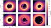 |
Fig. 10 Synthetic ALMA observations at 855 μm of the disc in model M9-3 (assuming a distance of 100 pc) at different times: prior (a and b), during (c and d), and after (e and f) a migration jump. The panels coincide with the ones in Fig. 5 but they show the intensity from simulated observations instead of surface density and are zoomed-in to the inner ± 100 au of the disc. Coordinate ticks are the same in all panels and values are given in arcseconds in the top left panel and the corresponding values in au are shown in the bottom left panel. The ellipse in the bottom right corner of each panel indicates the beam size of 33 × 30 mas. The location of the star is indicated by the small cross symbol in the centre. The current orbits of the two planets are marked by the dotted white ellipses and the planetary Hill spheres are indicated by the small circles. |
4.2 Synthetic imaging
We use the task simalma from the CASA-5.6.1 software to simulate the detectability of the various features present in the model. A combination of the antenna configurations alma.cycle5.8 and alma.cycle5.5 was chosen. The simulated observation time for configuration “8” is 4 h while the more compact configuration is integrated over a shorter time of 53 min.
A simple auto-cleaning procedure was applied to reduce the artificial artefacts from the incomplete uv-coverage. In the scope of this paper the prescription is sufficient for estimating the observability of the features of interest. Consistent with the radiative transfer model, the observed wavelength is simulated to be at 855 μm, corresponding to ALMA band 7. The resulting beam size is 33 × 30 mas. For model M9-3, the rms noise intensity ranges from 40 μJy beam−1 to 70 μJy beam−1. The synthetic images are shown in Fig. 10. In the rest of this section, we describe the different features that are visible in the synthetic images. All references are to Fig. 10, unless stating otherwise.
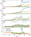 |
Fig. 11 Migration history (as in Fig. 3) for the PDS 70 models. A migration jump occurs for both equations of state in the case of a high-surface-density model (PDS70 ISO and PDS70 IRR). The model with a fifth of the surface density (PDS70 IRR M/5) shows only very moderate outward migration. The left vertical dotted line shows the time of planet release. The right vertical dotted line shows the time of the synthetic observations shown in Fig. 12. |
4.3 Features in synthetic images
Our synthetic images show a large inner hole in the disc which is growing over time. This can appear as a circular hole at some points in time (panels a and f of Fig. 10) or as an eccentric hole at other times (panels b–d). As we removed the dust artificially, the inner hole might actually be partially filled with dust and still be showing a visible inner disc. Because our cut-off radius is 26 au at maximum, such a system with an inner disc would show a large gap ranging from about 20 au in size for panel b to around 75 au for the disc in panel f. For an example where only part of the dust is removed, see the PDS 70 models in Fig. 12.
Our simulations produce a number of non-axisymmetric features in the synthetic observations. In the following sections, we investigate these in more detail. Emission from the location of the planets is clearly visible in the synthetic observations. Very localised, point-like features around the planet are visible either from a single planet (panels a, c, and d) or from both planets (panels b, e,and f). These emerge because of mass accumulations in the planets’ Hill spheres. During a migration jump (panels c and d), the outer planet is deeply embedded in the disc, and so no separate point-like emission is visible from the outer planet.
The vortex discussed in Sect. 3.4 is also visible in the synthetic images. It appears as a bright region on the right side of panel b causing a visible non-axisymmetric feature. Depending on the line-of-sight inclination of the disc and beam size, the asymmetry caused by the vortex can even be enhanced (see panels b and d of Fig. 12).
When the outer or inner planet gets close to the gap edge, the outer part of the spiral arm can be visible in the synthetic images, connecting the planet with the outer disc with a visible spur. This is the case for panels b, e and f with the outer planet and panels c and e with the inner planet.
At the time when the planets are released, there is still some material present in the L4 and L5 points of the outer planet. This is an artefact of the initialisation process. Although it is also visible in the synthetic observations (panel a), it does not constitute a realistically observable feature but rather an artefact of the initialisation and the assumption that dust and gas share the same spacial distribution. However, when the outer planet migrates back in during a migration jump, a substantial amount of material survives as a mass accumulation in Lagrangian point L5 (trailing theplanet). The accumulation is clearly visible in panel e. This feature can persist for more than 20 kyr as shown by its presence in panel f.
During times of high mass transfer through the common gap, surface density in the spiral arms in enhanced. Panels b, c, and e show clearsigns of spiral arms even in the synthetic images. The spiral arms of both planets are periodically cut off by the passing of the other planet and locally merge with parts of other spiral arms. This causes additional arc-like features such as the ones in panels b and e.
Another arc-like feature can be produced during the migration jump. Panels c and d show a void behind the planet in the lower right quadrant at a radius of approximately 75 au. These voids are 30° (panel c) to 60° (panel d) in width in the azimuthal direction and are caused by the gap being carved into the previously unperturbed disc during rapid outward migration (Pepliński et al. 2008).
Just after the migration jump (panel e), multiple substructures can be seen inside the orbits of the planets. This shows that more than one of the features presented above can exist in a disc at the same time.
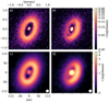 |
Fig. 12 Synthetic observations of the PDS 70 models. Disc mass increases from left to right and resolution decreases from top to bottom. For a lower disc mass, the appearance is smooth and symmetric, showing a large gap. At higher disc mass, azimuthal asymmetries appear and additional substructures emerge for higher resolution. Left column (a and c): low-disc-mass model (PDS70 IRR M/5) at t = 70.3 kyr (see vertical line in Fig. 11) and right column (b and d): high-disc-mass model (PDS70 IRR) at the same point in time. Top row (a and b): generated with the same angular resolution as Fig. 10 while only the smaller ALMA antenna configuration was used for the bottom row (c and d), resulting in a larger beam size. The beam size is indicated in the bottom right corner of each image. |
5 Modelling of a real system: PDS 70
PDS 70a is a 5.4 ± 1.0 Myr-old K7-type star with a mass of 0.76 ± 0.02 M⊙ and luminosity outflow L* = 0.35 ± 0.09 L⊙ (Müller et al. 2018). It is at a distance of 113.43 ± 0.52 pc (Gaia Collaboration 2018). Recently, it was found to host two giant planets, PDS 70b and PDS 70c, which were observed via direct imaging. Their orbits are close to a 2:1 MMR with distances of about ab = 20.6 ± 1.2 au and ac = 34.5 ± 2 au (Keppler et al. 2018; Haffert et al. 2019). The inner planet is believed to be more massive than the outer one while their mass estimates are still uncertain at Mb = 5−14 MJup (Keppler et al. 2018) and Mc = 4−12 MJup (Haffert et al. 2019). These masses were estimated by comparing photometry of the sources to synthetic colours from planet evolution models.
Recently, Bae et al. (2019) showed that ALMA dust continuum observations at 890 μm can be convincingly reproduced by a pair of outward migrating planets. These latter authors performed 2D locally isothermal hydrodynamical simulations with a temperature profile obtained from radiative transfer calculations and using a stellar mass of 0.85 M⊙ and two planets close to 2:1 MMR with masses of Mb = 10 MJup and Mc = 2.5 MJup. They found the system to be stable for 1 Myr while smoothly migrating outward.
We ran additional simulations to model PDS 70 in order to test whether migration jumps could occur in that system. The PDS 70 models differ only slightly from our standard M9-3 setup, that is, the stellar mass is lowered to M* = 0.76 M⊙. One PDS 70 simulation uses the locally isothermal equation of state (PDS70 ISO), while a second and third one use the ideal equation of state with irradiation from the star, like the IRR model above, with stellar luminosity L* = 0.35 ± 0.09 L⊙ (Müller et al. 2018). The first two models use the standard Σ(r) profile (PDS70 ISO, PDS70 IRR) and the last one has a five-times-smaller Σ (PDS70 IRR M/5). All three models were integrated for 100 kr and are included in Table 1. Our models have a higher surface density compared to the ones in Bae et al. (2019). At a distance of 40 au this amounts to Σ = 11.6 g cm−2 and Σ = 2.4 g cm−2 (PDS 70 IRR M/5) in our models compared to their Σ = 1 g cm−2.
5.1 Dynamical results
Figure 11 shows the dynamical outcome of the PDS 70 models. The model with a lighter disc (PDS70 IRR M/5) shows no special events. The inner planet migrates outward very slowly while the outer planet migrates inward until the system is locked into 2:1 MMR around t ≈ 80 kyr (54 kyr after planet release). The system then migrates slowly outward together, maintaining the 2:1 resonance. The inner planet moves less than 0.5 au over the remaining 20 kyr.
Both models with high Σ show one migration jump until the end of the simulation at 100 kyr. The outer planet first migrates inward for approximately 10 kyr until the planets lock in 2:1 MMR. Rapid outward migration then starts in both cases leading up to a migration jump 30 kyr later.
In the PDS70 ISO case, the outer planet travels 10 au during that time and a migration jump takes it out to nearly 70 au with a period commensurability of Pout∕Pin ≈ 4. During the 16 kyr duration of the migration jump, the inner planet travels out by 5 au, because the negative torque contribution from the outside is missing. Due to the fast outward migration of the inner planet, when the outer planet migrates back in from the jump, the location of the 2:1 MMR is much further out. When the system goes back into 2:1 MMR, the outer planet is at 60 au from which point outward migration continues.
The sibling simulation with a more realistic equation of state and irradiation from the star (PDS70 IRR) shows similar, though less extreme effects. The outer planet travels out by 4 au following the point at which the planets become locked into resonance 30 kyr before the migration jump is about to happen. The smaller migration jump moves the outer planet further out by 6–46 au, where it has a period commensurability of Pout∕Pin ≈ 2.75. Again, the migration jump takes around 16 kyr, but the inner planet only migrates approximately 1 au during that time. Thus the location of 2:1 MMR for the outer planet is further in, at 44 au, to where it migrates back over a time-span of 6 kyr (instead of jumping back) until it locks into 2:1 MMR again. The different stopping location of the jump between models PDS70 and PDS70 IRR does not seem to stem from a difference in aspect ratio. Indeed, the aspect ratio in model PDS70 IRR is nearly identical to the one in model IRR, which is displayed in Fig. B.2, and is close to 0.05 around 40 au, exactly as in the locally isothermal model.
Along with the migration jumps, both models with a higher surface density show the formation of a vortex outside the gap already when the planets lock into 2:1 MMR. In the PDS70 IRR model, the vortex survives the small migration jump and lives on until the end of the simulation. In the PDS70 ISO model, it lives until the migration jump when it is disrupted by the outer planet and does not form again during the simulation time.
5.2 Synthetic images
Similarly to the model outcomes presented in Sects. 4.1 and 4.2, the outcomes of the PDS 70 models are post-processed in order to allow a comparison to the observed system. A modification of the procedure was made regarding the temperature and radius of the central star which have been set to 3972 K and 1.26 R⊙, respectively (Keppler et al. 2018). The mass of the inner disc was reduced by a factor of 10−2 instead of 10−5 to keep some emission from the inner disc which can be seen in the observation (Keppler et al. 2019). We additionally apply an inclination angle of 51.7 degrees and a position angle of 156.7 degrees.
Figure 12 shows the synthetic observations of the model PDS70 IRR (panels b and d) and the model with lower disc mass PDS70 IRR M/5 (panels a and c), where the synthetic observations are calculated using two different ALMA antenna configurations. The first configuration (panels a and b) is unchanged from the one in Sect. 4.2. The second configuration (panels c and d) only uses the smaller alma.cycle5.5 antenna configuration which results in a larger beam size.
Because the inner disc is more massive in gas, our assumption of a gas to dust ratio of 100 results in a very bright inner disc for higher disc masses. For each configuration, the colour scale is chosen such that its maximum value is the maximum intensity from the low-disc-mass models (panels a and c). This is done to make the outer parts of the disc visible in both models on the same colour scale.
The low-mass disc at high resolution (panel a) shows a hole in the inner disc. This is due to the inner hole of the computational domain. In the high-disc-mass case (panel b) this is no longer visible due to the selection of the maximum value for the colour scale. For the smaller ALMA configuration with larger beam size (panels c and d), the hole is simply smeared out.
There isa clear difference between the model PDS70 IRR M/5 with lower disc mass and smooth outward migration (panels a and c) and model PDS70 IRR with higher disc mass and a migration jump (panels b and d). The low-disc-mass model (panels a and c) qualitatively reproduces the dust continuum observations presented in Keppler et al. (2019) showing the dust ring at a large distance from the star and a clearly visible and wide gap. Here, the location of the dust ring is closer in compared to the observations.
For a higher disc mass, the ring becomes azimuthally asymmetric with the right side being pronounced due to the existence of a vortex. Atlower resolution (panel d), only the brighter right side is visible. At higher resolution (panel b), additional substructure is visible in the disc; for example the spur feature is visible to the right of the centre. Also clearly visible is an arc-like feature in the gap in the bottom left quadrant. The arc is located closer to the centre of the gap and emerges because the spiral arm of the inner planet is enhanced in density at that point in time. During the previous orbits, the outer planetcame close to the outer gap edge on its eccentric orbit which results in a higher mass flow across its orbit. This higher mass flow across the orbit of the outer planet subsequently leads to higher densities in the spiral arm of the inner planet. Therefore, the arc is a result of the dynamic nature of the system with its high eccentricities.
6 Discussion
In this section, we discuss the implications of our findings, put them into context, and discuss their limitations. Results are discussed in reverse chronological order starting with our PDS 70 models (Sect. 6.1) and followed by the synthetic observations (Sect. 6.2), their implications (Sect. 6.3), and migration jumps (Sect. 6.4). We then go on to discuss simulation aspects such as the role of the inner boundary condition (Sect. 6.5) and choices concerning the equation of state and self-gravity (Sect. 6.6). We conclude by discussing the implications of our findings for transition discs (Sect. 6.7) and directly imaged systems of planets at large distances from their host stars (Sect. 6.8).
6.1 PDS 70
Our synthetic observations of the PDS 70 system show a dust ring at slightly smaller radii compared to Keppler et al. (2019). If we had simulated the system for a longer time, the pair of planets would have migrated further out also pushing the location of the ring further out. This way the synthetic models could be fine-tuned to match the actual observations.
In the case of PDS 70, our results suggest that no migration jump is happening in the system at this moment in time. This is likely due to the disc mass being lower than needed for migration jumps to happen, as the comparison between models PDS70 IRR and PDS70 IRR M/5 shows. Following this line of thought, our results might be used to put an upper limit on the disc mass. The disc mass must be lower than the one in model PDS70 IRR, Mdisc = 0.048 M⊙, at the time when the migration jump happens. We note that for simulations, the disc mass depends on the extent of the domain and the numbers quoted here refer to a disc with the inner and outer radius of our models, rin = 2.08 au and rout = 208 au. Scaled with a power-law profile as in Eq. (1), this corresponds to a surface density of Σ = 8.24 g cm−2 at 40 au which is in agreement with the Σ ≈1 g cm−2 at 40 au which has been used in models of PDS70 before (Keppler et al. 2018, 2019). Another upper bound could be obtained by verifying the non-existence of features due to gravitational instability such as fragmentation which would require even more massive discs. Our threshold is lower than this self-gravity-induced upper bound because our discs have a Σ which is lower than the value required for fragmentation. The Toomre Q parameter islarger than 1 at any location and time. The upper bound could likely be improved by performing a parameter study which is outof the reach of this work.
Given the age of PDS 70, namely 5.4 ± 1.0 Myr, it cannot beruled out that a migration jump happened at earlier times, and that the system relaxed back into a quieter state as the disc dispersed due to effects like photoevaporation or magnetically driven disc winds (Rodenkirch et al. 2020). Long-term simulations including disc dispersal effects would be required to answer this question.
In our synthetic images, we also observe the spur at the outer gap edge reported by Keppler et al. (2018, 2019) which has already been reproduced using a similar model to ours (Bae et al. 2019). Such a feature also appeared in our generic models (see Fig. 10 panels b, e, and f), suggesting that this kind of feature can generally appear for an outward migrating pair of planets.
6.2 Synthetic observations and dust treatment
In Sect. 4.2, we model dust emission by assuming a uniform dust-to-gas mass ratio of 10−2. Thus, we use gas dynamics as a proxy for dust dynamics. As a result, effects like dust drift, dust size filtration, and dust diffusion (Weber et al. 2018), which are probably at play in a protoplanetary disc, are not considered. The inclusion of a proper dust treatment might therefore change the appearance of some features in the synthetic images.
Nonetheless, similar features have been observed to also emerge when dust is handled properly. A dust ring growing in size because of outward migration of a pair of massive planets was reported by Marzari et al. (2019) for a close-in (inside 10 au) Jupiter–Saturn pair in a massive disc (Σ0(10 au) = 75 g cm−2 versus Σ0 (10 au) ≈ 46 g cm−2 here) and by Bae et al. (2019) for a model of the PDS 70 system with 10 and 2.5 MJup planets in a lighter disc (Σ0(10 au) ≈ 9 g cm−2). The latter study also found the PDS 70 spur feature (Keppler et al. 2019; Bae et al. 2019), supporting the idea that similar features also appear with proper dust treatment. However, to judge how dust dynamics influences the features found in our synthetic observations, simulations including dust treatment are needed. We plan to investigate this in a follow-up study.
We want to highlight that multiple distinct observational features can be created by the same planetary system at different points in time if the system exhibits sufficiently strong dynamic effects such as a migration jump. Except for the choice of planet mass ratio, all presented observational features emerged for a disc with standard parameters without the need of fine-tuning.
6.3 Observational signposts for dynamic effects
For our PDS 70 models (see Sect. 5), we observed non-axisymmetric features in the higher disc mass model. The higher surface density caused faster outward migration and thus a higher mass flow through the common gap. The first effect was the appearance of a vortex, visible as asymmetry in the intensity distribution (Figs. 12 b and d). The second effect was an arc-like feature in the gap region caused by an enhancement of density in the spiral arm of the inner planet. Together with the spur feature discussed above, if detected in real observations, these features might hint at outward migration and enhanced mass flow through the gap region.
Contrasting the smooth synthetic observations of our low-mass PDS 70 model, or the model by Bae et al. (2019) in which the planetary system undergoes smooth and slow outward migration, with our synthetic observations in Fig. 10, we can identify which features could be “signposts” for strong dynamical effects like migration jumps. We can identify these potential signposts as very eccentric holes or gaps, vortices, arc-shaped voids, mass accumulations in Lagrangian points, and visible spiral arms. The latter two might be the easiest to discover in real observations because they are located in the gap region where the surrounding emission is weak. Indeed, similar features such as an arc inside a gap have already been observed, for example in the disc of HD 163296 (Isella et al. 2018). Fast outward migration of a single planet might lead to comparable observational signatures such as arc-shaped voids behind the planet (Pepliński et al. 2008). Therefore, only the combinationof one of the signposts listed above with a large gap will provide a strong indication for a migration jump.
Our simulations show that a higher disc mass facilitates stronger planetary system dynamics. Thus, by pointing toward strong dynamic effects, these signposts might indirectly hint at a high gas mass.
6.4 Migration jumps
Migration jumps are introduced in Sect. 3.2. To our knowledge, we are the first to name, describe, and analyse this dynamical process in detail. We observed migration jumps for different resolutions (Appendix A), for different choices of equation of state and treatments of the energy equation (Sect. 5 and Appendix B), for different domain sizes (models L and L M/2), independent of accretion onto the planet (Sect. 3.5), for different choices of inner boundary conditions (models VB* and WD*), and for models with and without self-gravity (models SG and SG IRR). These tests reinforce our confidence that migration jumps are indeed a physical effect.
There isat least one example in the literature where migration jumps appeared in simulations. Figure 1 of Chametla et al. (2020) shows two migration jumps in their model 7b in which a Jupiter–Saturn pair (mass ratio 3:1) is migrating outwards in 3:2 MMRand experiences two small migration jumps between 5 and 8 au. This indicates that migration jumps can also happen for other types of MMRs, at smaller radii, and for planet masses down to a Jupiter–Saturn-sized pair. A natural question to ask refers to why migration jumps were not found before, in studies like Marzari et al. (2019) or Bae et al. (2019), for example.
For the case of Marzari et al. (2019), we repeated similar simulations with different boundary conditions and the domain size from 0.5 to 15 au. We found smooth outward migration at similar rates. In these simulations, the surface density, Σ, is about twice as high as in our model M9-3. The non-appearance of a migration jump is likely due to the non-existence of a vortex in these simulations. This is probably due to the smaller outer radius and the wave damping zone close to the outer boundary which prevents the formation of a vortex at the location where we would expect it by scaling down the location from our simulations. This suggests that vortices are important for the mechanism of migration jumps.
In the case of Bae et al. (2019), the non-appearance of migration jumps is very likely due to the lower value of Σ, which is comparable to that of our model M9-3 M/10 which also does not show a migration jump.
Migration jumps could have profound effects for planetary systems. During the jump, dust can be gravitationally scattered by the planets which might be a way to redistribute dust trapped in a pressure maximum and possibly even dust trapped in the vortex. We plan to perform simulations with embedded dust to explore these hypotheses.
A jump might also have significant effects for the accretion process as shown in Sect. 3.5. Mass accretion rates onto the planets can be enhanced by two orders of magnitude by moving the outer planet to regions outside the planet gap where the surface density is high. This in turn also increases the mass accretion onto the inner planet. Together this might provide a mechanism by which massive planets can accrete mass more efficiently by tapping into mass reservoirs far away from their initial orbit.
In our view, migration jumps are a composite phenomenon in which resonant outward migration via the Masset & Snellgrove (2001) mechanism, the interaction of a planet with a vortex, and the subsequently triggered type III rapid outward migration are combined to give rise to an emerging effect.
6.5 Planet ejections and internal boundary condition
Planet ejections occurred in models where an inner boundary different from outflow was used in combination with a disc centred in the centre of mass of the N-body system due to a numerical instability (Sect. 3.6). Our results suggest that if a viscous boundary, a reflective boundary, or wave-damping zones are used, the hydrodynamical simulation should be centred on the primary star. It might also be possible to adjust the boundary condition to follow the moving star in the other case, but we did not implement this more complicated feature. Such a dependence of the dynamical behaviour of planets on the treatment of the inner boundary, which lies well inside the actual realm of the planets, has been observed in other simulations of embedded planets, for example for the system GJ 876 (Crida et al. 2008; Cimerman et al. 2018). The outflow boundary condition seems to give more freedom to the inner disc by allowing a moving inner disc edge. Indeed, this boundary condition is also a good choice to simulate eccentric discs around binary stars (Thun & Kley 2018).
6.6 Equation of state and self-gravity
Recent studies have shown that radiative effects can play an important role for the spiral arm and gap structure in the case of low-mass planets where radiative effects cause significant changes compared to a purely locally isothermal assumption (Ziampras et al. 2020). In our case, we see a qualitatively similar behaviour for locally isothermal simulations and simulations considering radiative effects (see Appendix B). However, the size of migration jumps and the rate of outward migration depend on the inclusion of radiative effects in our PDS 70 models (Sect. 11). The appearance of migration jumps for both radiative and locally isothermal models hints at the dynamic nature of the process. Migration jumps are likely dominated by resonant N-body interactions pumping eccentricities and the interaction with the vortex formed outside the gap.
For reasons of simplicity and runtime, we neglected self-gravity in most of our simulations. Judging by the value of the Toomre Q parameter which stays above 1 at all times, the disc is not prone to fragmentation. However, other processes might be slightly altered when self-gravity is taken into account. Firstly, self-gravity might play a role in the migration of massive planets as is the case for low-mass planets (Ataiee & Kley 2020). Secondly, in our simulations, the occurrence of migration jumps coincides with the existence of a vortex. When self-gravity is considered, vortices will weaken and can stretch out even for low-mass discs as long as the Toomre Q parameter is lower than 50 or  (Lovelace & Hohlfeld 2013; Regály & Vorobyov 2017; Zhu & Baruteau 2016). Both conditions are fulfilled in the standard M9-3 model with Q ≈ 6 and h Q ≈ 0.3 for the initial profile at the location of the vortex.
Models SG and SG IRR with self-gravity enabled indeed show that there is no disc fragmentation, but stretching of the vortex. Hence, our finding that migration jumps still occur with self-gravity considered is one more indication that they are indeed a physical phenomenon.
6.7 Mass accretion and Type II transition discs
In all our models, mass accretion onto the star, as measured by the mass flow rate through the inner boundary, was higher (10−8 to 10−7 M⊙ yr−1) than the viscous mass accretion rate of the unperturbed disc (<10−8 M⊙ yr−1). The inner disc was building up mass over time in these models, showing higher surface densities compared to the initial profile. We suspect that mass transfer through the gap is enhanced by the “shoveling” mechanism (Sect. 3.5). As the outer planet comes close to the outer gap edge at apastron on its eccentric orbit, it scatters mass inwards. Additionally, outward migration must necessarily enhance mass flow through the gap. When the planets migrate outward, they gain angular momentum. Because angular momentum is conserved, the angular momentum gained by the planets has to be extracted from the gas requiring that some gas has to move from outside the gap (outside the planetary orbits) to inside the gap (inside the planetary orbits) to supply the angular momentum. This mechanism of shovelling matter from outside in is after all the basic mechanism behind the Masset–Snellgrove mechanism of outward migration, as the material crossing the joint gap is collected in the inner disc which generates the positive torque to drive the planets outward (Masset & Snellgrove 2001). Our models serve to quantify this process in more detail.
A particularly clear example of this mechanism is model L for which we reported the dependency of mass accretion through the gap on the direction of migration in Sect. 3.5. There, mass flow through the gap is present during both in- and outward migration but is strongly enhanced for the outward case. This means that the common gap formed by the planets is not an impermeable barrier for mass accretion. Model L illustrates that mass flow through the gap is possible for both directions of migration and that it can be enhanced by over one order of magnitude in the case of outward migration.
The large gap in dust emission reported in Sects. 4 and 5 (see also Marzari et al. 2019; Bae et al. 2019) together with an enhanced stellar mass accretion make outwardly migrating pairs of planets prime candidates for a consistent explanation of Type II transition discs (Owen & Clarke 2012) which feature large gaps or holes and high accretion rates at the same time.
6.8 Directly imaged planets at large distances
There are several examples of giant planets observed at large distances from their host star. At such large distances, in situ formation by gravitational instability is challenging (Zhu et al. 2012). Assuming they formed further in, it is still challenging to explain how they moved outwards over long distances, even though models based on the smooth outward resonant migration have been invoked to explain such systems (Pepliński et al. 2008; Crida et al. 2009; Kimmig et al. 2020). The advantage of our migration jumps is the very short timescale on which they occur and the large radial range covered.
PDS 70is one example, with the outer planet located at 35.5 ± 2 au (Haffert et al. 2019), for which outward migration seems a promising scenario, as a comparison with our simulations shows. In our simulations, the outer planet reaches distances from its host star of up to 133 au after 226 kyr, providing an explanation of how planets can reach such large distances from their host after being formed further inside. The actual process is likely a balance between speed of migration and dispersal of the disc, allowing for a range of final locations.
HR 8799 is another famous example of a directly observed planetary system that features a chain of four planets which might be in 8:4:2:1resonance (Marois et al. 2010; Goździewski & Migaszewski 2014). There, the outer planet HR 8799 b is located around 70 au (Wang et al. 2018). It is unclear whether or not outward migration in resonance can also produce such an intricate system, yet formation of the planets closer to the star followed by outward migration should be considered as a formation scenario. More extended simulations with more planets are needed to elucidate this problem.
7 Summary
We studied the dynamical evolution of a system of two massive planets (in a mass range of 3–9 MJup) embedded in a protoplanetary disc using two-dimensional, viscous hydrodynamical simulations carried out with the FARGO code. The planets were treated as smoothed point masses that in some simulations were allowed to accrete mass which was added to their dynamical mass. For the disc, we assumed either a locally isothermal equation or a more realistic situation where we solved for an energy equation that included viscous heating, radiative cooling, and stellar irradiation.
Concerning the migration of the planets, we found two different basic behaviours depending on the mass order of the two planets. In the case of a more massive outer planet, the planets migrate inward engaged in 2:1 MMR. For a more massive inner planet with mass ratios of 2:1 or 3:1, we find outward migration of both planets, again engaged in a 2:1 MMR. As found before, this resonant migration process, originally described by Masset & Snellgrove (2001) for the Jupiter–Saturn system, can lead to a resonant outward migration in 2:1 MMR in the case of massive planets (Pepliński et al. 2008; Crida et al. 2009).
The new feature that we discovered is an occurrence of what we call a “migration jump”. A migration jump is a composite phenomenon in which outward migration in resonance and interaction with a vortex cause conditions such that type III rapid outward migration is triggered. The outer (lighter) planet covers a large radial distance on a very short timescale, for example from 40 to 72 au in only 5000 yr; see Fig. 4. The phase of outward migration is usually followed by a phase of inward migration back into the initial resonant configuration. Migration jumps are a generic, robust feature of our models. They occur for different equations of state and accretion rates onto the planet, with or without self-gravity, and for different resolutions, as long as the surface density of the disc is sufficiently high.
In addition to the dynamical behaviour of the embedded planets, we monitored the mass accretion onto the central star, as this is a standard observable feature in transition discs (Owen 2016). For our models we find that during the smooth outward migration phase of the resonantly locked planet pair the accretion rate is significantly higher than in the situation when the outer planet has a higher mass and the planets migrate inward. During the outward migration phases the planetary system gains angular momentum which is lost by the disc. As a consequence, the disc material moves inwards and is “shovelled” towards the star by the pair of planets. This increases the mass flow rate onto the star by more than one order of magnitude, much higher than in the regular phases of smooth inward migration. This effect can be even more enhanced during the short phase of a migration jump; see Figs. 7 and 9. A combination of outward migration and high stellar mass accretion, as found in our models, could serve as a consistent explanation for the phenomenon of Type II transition discs with large inner holes and nevertheless high stellar accretion rates (Owen & Clarke 2012).
Using the outcome of our hydrodynamical models, we calculated synthetic images that show a surprising variety of non-axisymmetric features appearing over time in a single system; see Fig. 10. Depending on their dynamical state, a bright ring just beyond the planets was seen, followed by vortex structures, and then additional structures in the main gap created by the planets. These initial images were based on a constant dust-to-gas ratio and for more realistic cases the dust dynamics will have to be followed simultaneously to the gas dynamics. Nevertheless, the initial models provide insight into the possible observational effects generated by the planets. In our study, we also included models with parameters reminiscent of the system PDS 70, which contains two massive embedded planets. From our synthetic images for this system we may conclude that it does not currently undergo a migration jump but might very well be in a phase of outward migration, compatible with Bae et al. (2019). The non-occurrence of the signposts of a migration jump indicates a disc mass lower than Mdisc < 0.048 M⊙ for a disc extending out to 200 au which serves an independent upper bound compatible with radiative transfer models reproducing the observationsof the system (Keppler et al. 2018, 2019). A more detailed comparison between simulations and observations will have to consider dust embedded in the disc. From our models we can finally conclude that Type II transition discs with large inner holes but significant stellar accretion are indeed signposts for highly dynamic embedded planetary systems.
Acknowledgements
All authors acknowledge funding from the DFG research group FOR 2634 “’Planet Formation Witnesses and Probes: Transition Disks” under grant DU 414/22-1 and KL 650/29-1, 650/30-1. The authors acknowledge support by the High Performance and Cloud Computing Group at the Zentrum für Datenverarbeitung of the University of Tübingen, the state of Baden-Württemberg through bwHPC and the German Research Foundation (DFG) through grant INST 37/935-1 FUGG. Plots in this paper were made with the Python library matplotlib (Hunter 2007).
Appendix A Convergence with resolution
To test convergence of the simulations with respect to spatial resolution, we ran a model with the 2D resolution lowered andincreased by a factor of two, i.e. in each direction the resolution is changed by a factor of  . Model M9-3 HR has Nr × Nϕ = (426, 580) and model M9-3 DR has Nr × Nϕ = 851 × 1161 cells. They are otherwise identical to the M9-3 model which has Nr × Nϕ = 602 × 821 cells.
A comparison of the planet migration for the three cases is shown in Fig. A.1. The overall qualitative behaviour isthe same; the most noticeable difference is the time at which the migration jump occurs. For the first jump, this is only slightlydifferent. Since the changes are small, we conclude that the simulations are converged with respect to resolution. In fact, the lower resolution is already sufficient to resolve the dynamics.
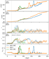 |
Fig. A.1 Migration history of models with standard, double (DR), and half (HR) 2D resolution to test convergence with spacial resolution. The panels show, from top to bottom, evolution of the semi-major axis of the outer planet, same for the inner planet, their eccentricities (middle and following panel), and their period ratio. |
Appendix B Dependence on equation of state
Using the locally isothermal equation of state is a valid approximation in the case of low optical thickness and negligible viscous heating compared to stellar irradiation. For the outer disc region, in which the planets in our simulations are located, thisshould be well justified. To test the assumption, we ran additional simulations where the energy equation is solved and viscous heating and cooling from the disc surfaces are included as in Müller & Kley (2012), and irradiation from the star is treated analogously to Ziampras et al. (2020) with their choices of parameters. Additionally, we repeated the standard M9-3 with a radial temperature profile that is set by stellar irradiation, which resembles the temperature profile in model IRR very well resulting in a flared disc (see Fig. B.2 below).
Figure B.1 shows a comparison of the migration history between the reference model M9-3 and the irradiation model IRR. Although the outward migration happens with a slower speed, a migration jump still occurs. Model IRR shows a first event at around 80 kyr where the eccentricity of the outer planet suddenly drops from 0.2 down to small values, but only jumps about 5 au. A second event occurs around 170 kyr where the outer planet jumps 45 au, comparable to the migration jumps observed in the M9-3 run. Model FLARE, which employs a locally isothermal equation of state, first follows the IRR model but instead of the failed small jump at 80 kyr it undergoes a full large jump. The comparison shows that, although details such as the migration rate depend on the aspect ratio profile, migration jumps appear also for flared discs.
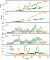 |
Fig. B.1 Comparison of the migration history of the standard M9-3 model and the more realistic and radiative model IRR and the model FLARE. Panels as in Fig. A.1. |
Figure B.2 shows the temperature and aspect ratio profiles for the three models. Around the region where the planets are located, the aspect ratios are comparable with values around 0.05. However, at the location where the planet jumps happens, h has increased to ~0.07 for the IRR and FLARE models. This might explain the difference in amplitude and period ratios during the migration jump. Finally, as there are only small qualitative differences, we conclude that the locally isothermal assumption is justified in this case to capture the most important dynamics.
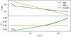 |
Fig. B.2 Temperature (top) and aspect ratio H ∕ r (bottom) forthe standard model M9-3, model IRR and model FLARE at 200 kyr. |
Appendix C Identification of the vortex
During the periods of resonant outward migration, a banana-shaped overdensity appears just outside the common gap. In this section, we analyse the snapshot in panel b of Fig. 5 of model M9-3 in more detail.
Figure C.1 shows the vortensity ω∕Σ normalised by its value from the initial profile. The numerator is the vorticity, which is defined as the z-component of the curl of the velocity,  . The orbits of both planets are shown as a dotted green line and the locations of the planets are indicated by the green crosses. By dividing the current value of the vortensity by the initial one at each location, the dependence on the steepness of the initial density profile and the background vorticity of the Keplerian disc are factored out. This results in a clear picture of what happens locally with the velocity field. A vortex in a disc appears as a region of lower vortensity as compared to its surroundings, due to its anticyclonic nature as seen in Fig. 6. This clearly identifies the overdensity at 59 au as a vortex.
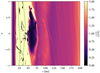 |
Fig. C.1 Vortensity normalized by the initial vortensity in r−ϕ coordinates for a ±100 au zoom-in to panel b of Fig. 5. The overdensity appears as a region of lower vortensity compared to its surroundings indicating that it is indeed a vortex. The orbits of the planets are shown as dotted green lines and the location of each planet is indicated by a small green cross symbol. |
References
- Alexander, R. D., Clarke, C. J., & Pringle, J. E. 2006, MNRAS, 369, 216 [NASA ADS] [CrossRef] [Google Scholar]
- Andrews, S. M., Huang, J., Pérez, L. M., et al. 2018, ApJ, 869, L41 [NASA ADS] [CrossRef] [Google Scholar]
- Ataiee, S., & Kley, W. 2020, A&A, 635, A204 [CrossRef] [EDP Sciences] [Google Scholar]
- Ataiee, S., Pinilla, P., Zsom, A., et al. 2013, A&A, 553, L3 [NASA ADS] [CrossRef] [EDP Sciences] [Google Scholar]
- Bae, J., Zhu, Z., Baruteau, C., et al. 2019, ApJ, 884, L41 [NASA ADS] [CrossRef] [Google Scholar]
- Baruteau, C. 2008, Theses, Observatoire de Paris [Google Scholar]
- Birnstiel, T., Dullemond, C. P., Zhu, Z., et al. 2018, ApJ, 869, L45 [NASA ADS] [CrossRef] [Google Scholar]
- Calvet, N., D’Alessio, P., Hartmann, L., et al. 2002, ApJ, 568, 1008 [NASA ADS] [CrossRef] [Google Scholar]
- Chametla, R. O., D’Angelo, G., Reyes-Ruiz, M., & Sánchez-Salcedo, F. J. 2020, MNRAS, 492, 6007 [CrossRef] [Google Scholar]
- Cimerman, N. P., Kley, W., & Kuiper, R. 2018, A&A, 618, A169 [CrossRef] [EDP Sciences] [Google Scholar]
- Crida, A., Morbidelli, A., & Masset, F. 2007, A&A, 461, 1173 [NASA ADS] [CrossRef] [EDP Sciences] [Google Scholar]
- Crida, A., Sándor, Z., & Kley, W. 2008, A&A, 483, 325 [NASA ADS] [CrossRef] [EDP Sciences] [Google Scholar]
- Crida, A., Masset, F., & Morbidelli, A. 2009, ApJ, 705, L148 [NASA ADS] [CrossRef] [Google Scholar]
- Cumming, A., Butler, R. P., Marcy, G. W., et al. 2008, PASP, 120, 531 [CrossRef] [Google Scholar]
- D’Alessio, P., Hartmann, L., Calvet, N., et al. 2005, ApJ, 621, 461 [NASA ADS] [CrossRef] [MathSciNet] [Google Scholar]
- de Juan Ovelar, M., Min, M., Dominik, C., et al. 2013, A&A, 560, A111 [NASA ADS] [CrossRef] [EDP Sciences] [Google Scholar]
- de Val-Borro, M., Edgar, R. G., Artymowicz, P., et al. 2006, MNRAS, 370, 529 [NASA ADS] [CrossRef] [Google Scholar]
- Dodson-Robinson, S. E., & Salyk, C. 2011, ApJ, 738, 131 [CrossRef] [Google Scholar]
- Dong, R., & Dawson, R. 2016, ApJ, 825, 77 [CrossRef] [Google Scholar]
- Dubrulle, B., Morfill, G., & Sterzik, M. 1995, Icarus, 114, 237 [NASA ADS] [CrossRef] [Google Scholar]
- Dullemond, C. P., Juhasz, A., Pohl, A., et al. 2012, Astrophysics Source Code Library [record ascl:1202.015] [Google Scholar]
- Dürmann, C., & Kley, W. 2017, A&A, 598, A80 [NASA ADS] [CrossRef] [EDP Sciences] [Google Scholar]
- Espaillat, C., Muzerolle, J., Najita, J., et al. 2014, Protostars and Planets VI, eds. H. Beuther, R. S. Klessen, C. P. Dullemond, & T. Henning (Tucson, AZ: University of Arizona Press), 497 [Google Scholar]
- Forgács-Dajka, E., Sándor, Z., & Érdi, B. 2018, MNRAS, 477, 3383 [Google Scholar]
- Gaia Collaboration (Brown, A. G. A., et al.) 2018, A&A, 616, A1 [NASA ADS] [CrossRef] [EDP Sciences] [Google Scholar]
- Goździewski,K., & Migaszewski, C. 2014, MNRAS, 440, 3140 [NASA ADS] [CrossRef] [Google Scholar]
- Haffert, S. Y., Bohn, A. J., de Boer, J., et al. 2019, Nat. Astron., 3, 749 [Google Scholar]
- Hayashi, C. 1981, Prog. Theor. Phys. Suppl., 70, 35 [NASA ADS] [CrossRef] [MathSciNet] [Google Scholar]
- Hendler, N. P., Pinilla, P., Pascucci, I., et al. 2018, MNRAS, 475, L62 [NASA ADS] [CrossRef] [Google Scholar]
- Ho, P. 2016, Nature, 530, 169 [CrossRef] [Google Scholar]
- Huélamo, N., Lacour, S., Tuthill, P., et al. 2011, A&A, 528, L7 [NASA ADS] [CrossRef] [EDP Sciences] [Google Scholar]
- Hunter, J. D. 2007, Comput. Sci. Eng., 9, 90 [NASA ADS] [CrossRef] [Google Scholar]
- Isella, A., Huang, J., Andrews, S. M., et al. 2018, ApJ, 869, L49 [NASA ADS] [CrossRef] [Google Scholar]
- Keppler, M., Benisty, M., Müller, A., et al. 2018, A&A, 617, A44 [NASA ADS] [CrossRef] [EDP Sciences] [Google Scholar]
- Keppler, M., Teague, R., Bae, J., et al. 2019, A&A, 625, A118 [NASA ADS] [CrossRef] [EDP Sciences] [Google Scholar]
- Kimmig, C. N., Dullemond, C. P., & Kley, W. 2020, A&A, 633, A4 [CrossRef] [EDP Sciences] [Google Scholar]
- Koller, J., Li, H., & Lin, D. N. C. 2003, ApJ, 596, L91 [NASA ADS] [CrossRef] [Google Scholar]
- Lovelace, R. V. E., & Hohlfeld, R. G. 2013, MNRAS, 429, 529 [NASA ADS] [CrossRef] [Google Scholar]
- Manara, C. F., Testi, L., Natta, A., et al. 2014, A&A, 568, A18 [NASA ADS] [CrossRef] [EDP Sciences] [Google Scholar]
- Marois, C., Zuckerman, B., Konopacky, Q. M., Macintosh, B., & Barman, T. 2010, Nature, 468, 1080 [NASA ADS] [CrossRef] [PubMed] [Google Scholar]
- Marzari, F., Baruteau, C., & Scholl, H. 2010, A&A, 514, L4 [NASA ADS] [CrossRef] [EDP Sciences] [Google Scholar]
- Marzari, F., D’Angelo, G., & Picogna, G. 2019, AJ, 157, 45 [CrossRef] [Google Scholar]
- Masset, F. 2000, A&AS, 141, 165 [NASA ADS] [CrossRef] [EDP Sciences] [Google Scholar]
- Masset, F., & Snellgrove, M. 2001, MNRAS, 320, L55 [NASA ADS] [CrossRef] [Google Scholar]
- McMullin, J. P., Waters, B., Schiebel, D., Young, W., & Golap, K. 2007, ASP Conf. Ser., 376, 127 [Google Scholar]
- Muley, D., Fung, J., & van der Marel, N. 2019, ApJ, 879, L2 [CrossRef] [Google Scholar]
- Müller, T. W. A., & Kley, W. 2012, A&A, 539, A18 [NASA ADS] [CrossRef] [EDP Sciences] [Google Scholar]
- Müller, T. W. A., & Kley, W. 2013, A&A, 560, A40 [NASA ADS] [CrossRef] [EDP Sciences] [Google Scholar]
- Müller, T. W. A., Kley, W., & Meru, F. 2012, A&A, 541, A123 [NASA ADS] [CrossRef] [EDP Sciences] [Google Scholar]
- Müller, A., Keppler, M., Henning, T., et al. 2018, A&A, 617, L2 [NASA ADS] [CrossRef] [EDP Sciences] [Google Scholar]
- Owen, J. E. 2016, PASA, 33, e005 [NASA ADS] [CrossRef] [Google Scholar]
- Owen, J. E., & Clarke, C. J. 2012, MNRAS, 426, L96 [NASA ADS] [CrossRef] [Google Scholar]
- Paardekooper,S. J., & Mellema, G. 2004, A&A, 425, L9 [NASA ADS] [CrossRef] [EDP Sciences] [Google Scholar]
- Pepliński, A., Artymowicz, P., & Mellema, G. 2008, MNRAS, 387, 1063 [NASA ADS] [CrossRef] [Google Scholar]
- Pinilla, P., de Juan Ovelar, M., Ataiee, S., et al. 2015, A&A, 573, A9 [NASA ADS] [CrossRef] [EDP Sciences] [Google Scholar]
- Regály, Z., & Vorobyov, E. 2017, MNRAS, 471, 2204 [NASA ADS] [CrossRef] [Google Scholar]
- Reggiani, M., Christiaens, V., Absil, O., et al. 2018, A&A, 611, A74 [NASA ADS] [CrossRef] [EDP Sciences] [Google Scholar]
- Rein, H., & Liu, S. F. 2012, A&A, 537, A128 [NASA ADS] [CrossRef] [EDP Sciences] [Google Scholar]
- Rice, W. K. M., Armitage, P. J., Wood, K., & Lodato, G. 2006, MNRAS, 373, 1619 [Google Scholar]
- Rodenkirch, P. J., Klahr, H., Fendt, C., & Dullemond, C. P. 2020, A&A, 633, A21 [CrossRef] [EDP Sciences] [Google Scholar]
- Sándor, Z., Kley, W., & Klagyivik, P. 2007, A&A, 472, 981 [NASA ADS] [CrossRef] [EDP Sciences] [Google Scholar]
- Shakura, N. I., & Sunyaev, R. A. 1973, A&A, 500, 33 [NASA ADS] [Google Scholar]
- Shu, F. H., Johnstone, D., & Hollenbach, D. 1993, Icarus, 106, 92 [NASA ADS] [CrossRef] [Google Scholar]
- Thun, D., & Kley, W. 2018, A&A, 616, A47 [NASA ADS] [CrossRef] [EDP Sciences] [Google Scholar]
- van der Marel,N., van Dishoeck, E. F., Bruderer, S., Pérez, L., & Isella, A. 2015, A&A, 579, A106 [NASA ADS] [CrossRef] [EDP Sciences] [Google Scholar]
- van der Marel, N., van Dishoeck, E. F., Bruderer, S., et al. 2016, A&A, 585, A58 [NASA ADS] [CrossRef] [EDP Sciences] [Google Scholar]
- Varnière, P., Blackman, E. G., Frank, A., & Quillen, A. C. 2006, ApJ, 640, 1110 [NASA ADS] [CrossRef] [Google Scholar]
- Wang, J. J., Graham, J. R., Dawson, R., et al. 2018, AJ, 156, 192 [Google Scholar]
- Ward, W. R. 1997, Icarus, 126, 261 [Google Scholar]
- Weber, P., Benítez-Llambay, P., Gressel, O., Krapp, L., & Pessah, M. E. 2018, ApJ, 854, 153 [NASA ADS] [CrossRef] [Google Scholar]
- Zhu, Z., & Baruteau, C. 2016, MNRAS, 458, 3918 [NASA ADS] [CrossRef] [Google Scholar]
- Zhu, Z., Nelson, R. P., Hartmann, L., Espaillat, C., & Calvet, N. 2011, ApJ, 729, 47 [NASA ADS] [CrossRef] [Google Scholar]
- Zhu, Z., Hartmann, L., Nelson, R. P., & Gammie, C. F. 2012, ApJ, 746, 110 [NASA ADS] [CrossRef] [Google Scholar]
- Ziampras, A., Ataiee, S., Kley, W., Dullemond, C. P., & Baruteau, C. 2020, A&A, 633, A29 [NASA ADS] [CrossRef] [EDP Sciences] [Google Scholar]
All Tables
All Figures
|
Fig. 1 Initial conditions for the disc around the 1 M⊙ star used in our simulations (blue). These are compared to the initial conditions of the disc in Bae et al. (2019) (green) in which the PDS70 system (0.85 M⊙ star) was modelled. For context, the surface density of the minimum mass solar nebula (MMSN; Hayashi 1981) is plotted in orange. Physical initial conditions after the equilibration phase (see Fig. 2) at t = 26 kyr are shown for model M9-3 as a dashed blue line. The panels, from top to bottom, show the radial profile of the: surface density, viscous mass accretion rate (Ṁdisc = 3πΣν with α = 10−3), temperature, and aspect ratio. The initial location of the planets are marked by the vertical, dotted lines which span over all panels and are indicated by the red and cyan circles. |
| In the text | |
|
Fig. 2 Flow chart illustrating the equilibration and simulation phase. The disc properties are initialised according to the power laws in Eqs. (1) and (2). During the equilibration process (taking 26 kyr, equivalent to 274 orbits at the initial location of the inner planet) where the disc begins to “feel” the planets, the density profile changes significantly; see the first panel of Fig. 1 for the difference, where the equilibrated profile is shown as the dashed blue line. |
| In the text | |
|
Fig. 3 Migration history for a selection of models described in Table 1 to highlight the different possible dynamical evolution of the embedded planets. The panels show, from top to bottom, the evolution of: the semi-major axis, a, of the outer and inner planet, their eccentricities, e, and their period ratio. The release time of the planets is marked by the vertical dotted line. Most prominent is the occurrence of fast outward migration (migration jump) for model M9-3 (blue) between 60 and 80 kyr, and a double orbit swap at 110 kyr followed by a migration jump for model M9-4.5. At the time of the double orbit swap at t ~ 110 kyr, ein = 0.38 and eout = 0.58. They are cut out to increase the visibility of the rest of the data. |
| In the text | |
|
Fig. 4 Zoom-in on a migration jump in model M9-3 including the time leading up to and following the event. The panels show, from top to bottom, the evolution of: the semi-major axis of both planets, their eccentricities, the 2:1 MMR angles,
|
| In the text | |
|
Fig. 5 Snapshots of the surface density for model M9-3 showing the disc at different times: prior (panels a and b), during (c and d), and after (e and f) a migration jump. The current orbits of the two planets are marked by the dotted white ellipses and the planetary Hill spheres are indicated by the small circles. Coordinate labels show the position in au. The snapshots are rotated to have the outer planet fixed on the horizontal axis to the right of the origin. Time inside the simulation is shown in the upper right corner. The time of a particular snapshot in the time-line of the simulation can be located on the annotated vertical lines in Fig. 4. For synthetic observations of the snapshots, see Fig. 10. |
| In the text | |
|
Fig. 6 Zoom-in on panel b of Fig. 5 showing the surface density and velocity streamlines. The streamlines are computed in a frame corotating with the disc at 59 au. The streamlines are closed in the region indicated by the black arrow, showing that the overdensity is a vortex. The orbits of the planets are indicated as the green dotted lines. |
| In the text | |
|
Fig. 7 Evolution of accretion rates, migration, and eccentricities for the models with planetary accretion.Then panels show from top to bottom: the semi-major axis of both planets, ain/out, the eccentricity of the inner planet and that of the outer planet, ein/out, planetary mass accretion rate onto the inner and outer planet, Ṁin/out, and the mass accretion rate onto the star smoothed with a moving average of length 1.185 kyr, Ṁ*. The vertical dashed lines indicate events of interest and are referred to in Sect. 3.5. Model A0.0 is an alias for model M9-3. |
| In the text | |
|
Fig. 8 Evolution of the mass accreted onto the planets and the star and the disk mass for the models with planetary accretion. The panels show from top to bottom: the mass accreted onto the inner and outer planet, Macc,pl, the mass which leaves the disc through the inner domain, Macc, *, (i.e. the mass that would be accreted onto the star, but which is not added to it in the simulations), and the evolution of the total disc mass, Mdisc. The evolution of Mdisk also includes the mass leaving the outer domain. The values are in units of the initial mass of the respective object for the accreted masses and in stellar masses for the disc mass. The dashed vertical lines correspond to the ones in Fig. 7. |
| In the text | |
|
Fig. 9 Migration and accretion for model L showing the orbit swap and how Ṁ* depends on the direction of migration. The panels show (top) semi-major axis, a, (middle) eccentricity, e, and (bottom) migration onto the star Ṁ*. The verticaldashed line indicates the time when planets are allowed to migrate. |
| In the text | |
|
Fig. 10 Synthetic ALMA observations at 855 μm of the disc in model M9-3 (assuming a distance of 100 pc) at different times: prior (a and b), during (c and d), and after (e and f) a migration jump. The panels coincide with the ones in Fig. 5 but they show the intensity from simulated observations instead of surface density and are zoomed-in to the inner ± 100 au of the disc. Coordinate ticks are the same in all panels and values are given in arcseconds in the top left panel and the corresponding values in au are shown in the bottom left panel. The ellipse in the bottom right corner of each panel indicates the beam size of 33 × 30 mas. The location of the star is indicated by the small cross symbol in the centre. The current orbits of the two planets are marked by the dotted white ellipses and the planetary Hill spheres are indicated by the small circles. |
| In the text | |
|
Fig. 11 Migration history (as in Fig. 3) for the PDS 70 models. A migration jump occurs for both equations of state in the case of a high-surface-density model (PDS70 ISO and PDS70 IRR). The model with a fifth of the surface density (PDS70 IRR M/5) shows only very moderate outward migration. The left vertical dotted line shows the time of planet release. The right vertical dotted line shows the time of the synthetic observations shown in Fig. 12. |
| In the text | |
|
Fig. 12 Synthetic observations of the PDS 70 models. Disc mass increases from left to right and resolution decreases from top to bottom. For a lower disc mass, the appearance is smooth and symmetric, showing a large gap. At higher disc mass, azimuthal asymmetries appear and additional substructures emerge for higher resolution. Left column (a and c): low-disc-mass model (PDS70 IRR M/5) at t = 70.3 kyr (see vertical line in Fig. 11) and right column (b and d): high-disc-mass model (PDS70 IRR) at the same point in time. Top row (a and b): generated with the same angular resolution as Fig. 10 while only the smaller ALMA antenna configuration was used for the bottom row (c and d), resulting in a larger beam size. The beam size is indicated in the bottom right corner of each image. |
| In the text | |
|
Fig. A.1 Migration history of models with standard, double (DR), and half (HR) 2D resolution to test convergence with spacial resolution. The panels show, from top to bottom, evolution of the semi-major axis of the outer planet, same for the inner planet, their eccentricities (middle and following panel), and their period ratio. |
| In the text | |
|
Fig. B.1 Comparison of the migration history of the standard M9-3 model and the more realistic and radiative model IRR and the model FLARE. Panels as in Fig. A.1. |
| In the text | |
|
Fig. B.2 Temperature (top) and aspect ratio H ∕ r (bottom) forthe standard model M9-3, model IRR and model FLARE at 200 kyr. |
| In the text | |
|
Fig. C.1 Vortensity normalized by the initial vortensity in r−ϕ coordinates for a ±100 au zoom-in to panel b of Fig. 5. The overdensity appears as a region of lower vortensity compared to its surroundings indicating that it is indeed a vortex. The orbits of the planets are shown as dotted green lines and the location of each planet is indicated by a small green cross symbol. |
| In the text | |
Current usage metrics show cumulative count of Article Views (full-text article views including HTML views, PDF and ePub downloads, according to the available data) and Abstracts Views on Vision4Press platform.
Data correspond to usage on the plateform after 2015. The current usage metrics is available 48-96 hours after online publication and is updated daily on week days.
Initial download of the metrics may take a while.