| Issue |
A&A
Volume 624, April 2019
|
|
|---|---|---|
| Article Number | A100 | |
| Number of page(s) | 10 | |
| Section | Interstellar and circumstellar matter | |
| DOI | https://doi.org/10.1051/0004-6361/201834700 | |
| Published online | 19 April 2019 | |
In-depth study of the hypercompact H II region G24.78+0.08 A1★,★★
1
INAF, Osservatorio Astrofisico di Arcetri,
Largo E. Fermi 5,
50125 Firenze, Italy
e-mail: cesa@arcetri.astro.it
2
I. Physikalisches Institut, Universität zu Köln,
Zülpicher Strasse 77,
50937 Köln, Germany
3
Institut de Radioastronomie Millimétrique (IRAM),
300 rue de la Piscine,
38406 Saint Martin d’Hères, France
Received:
21
November
2018
Accepted:
6
February
2019
Context. The earliest phases of the evolution of a massive star are closely related to the developement of an H II region. Hypercompact H II regions are the most interesting in this respect because they are very young, and hence best suited to study the beginning of the expansion of the ionised gas inside the parental core.
Aims. We have analysed the geometrical and physical structure of the hypercompact H II region G24.78+0.08 A1, making use of new continuum and hydrogen recombination line data (H41α, H63α, H66α, H68α) and data from the literature (H30α, H35α).
Methods. We fit the continuum spectrum with a homogenous, isothermal shell of ionised gas at 104 K and derive the size of the H II region and the Lyman continuum luminosity of the ionising star. We also fit the recombination line spectra emitted from the same shell with a model taking into account expansion at constant speed.
Results. The best fits to the continuum and line spectra allow the derivation of the Lyman continuum luminosity of the ionising star, H II region size, geometrical thickness of the shell, and expansion velocity. Comparison between the 5 cm and 7 mm brightness temperature distributions demonstrates that a thin layer of ionised gas of a few 1000 K at the surface of the H II region is necessary to reproduce the morphology of the continuum emission at both wavelengths.
Conclusions. We confirm that the G24 A1 hypercompact H II region consists of a thin shell ionised by an O9.5 star. The shell is expanding at a speed comparable to the sound speed in the ionised gas. The radius of the H II region exceeds the critical value needed to trap the ionised gas by the gravitational field of the star, consistent with the observed expansion.
Key words: stars: early-type / HII regions / ISM: individual objects: G24.78+0.08 / stars: winds, outflows
A copy of the reduced images (FITS files) is available at the CDS via anonymous ftp to cdsarc.u-strasbg.fr (130.79.128.5) or via http://cdsarc.u-strasbg.fr/viz-bin/qcat?J/A+A/624/A100
© ESO 2019
1 Introduction
Understanding the earliest stages of the evolution of massive stars is of pivotal importance to shed light on their formation process and to investigate the pristine characteristics of their natal environments. Hypercompact (HC) H II regions provide us with an important piece of information in this context. They represent the first step in the ionisation/expansion of an ionised region around a newly born early type star, as indicated by their physical parameters. While the distinction between HC and other H II regions (ultracompact, compact, and extended) is not sharp and the classification is mostly based on their sizes and emission measures (typically ≲0.03 pc and ≳1010 pc cm−6 for HC H II regions; see Kurtz 2005), HC H II regions present an interesting peculiarity (Sewilo et al. 2004): the radio recombination lines (RRLs) emitted from these objects are often significantly broader than expected for pure thermal and pressure broadening and turbulence in the ionised gas appears insufficient to explain the observed line widths.
All the above suggests that in HC H II regions the ionised gas is undergoing systematic, large-scale motions. Infall, expansion, and rotation have all been observed in some of these objects (Sollins et al. 2005; Klaassen et al. 2018; Moscadelli et al. 2018, hereafter M2018). Some models (Peters et al. 2010; Galván-Madrid et al. 2011) even predict flickering of the continuum flux due to oscillations of the H II region led by the complex interaction between the gravitationally unstable accretion flow and the ionising radiation of the star. Studying the morphology and radio emission from these objects in their early stages will help to verify the validity of these models. In particular, HC H II regions are bound to play an important role in this context. However, because of their small angular sizes, the mere detection of such regions has been difficult and time consuming, and even more so their detailed study. Thanks to new or upgraded instruments such as the Karl G. Jansky Very Large Array (VLA), the e-MERLIN interferometer, the NOrthern Extended Millimeter Array (NOEMA), and the Atacama Large Millimeter/submillimeter Array (ALMA) the situation is rapidly changing and it is now possible to detect and image the RRL emission and resolve the free-free continuum emission from the ionised gas in many of these objects (e.g. Klaassen et al. 2018).
In this article, we focus on the HC H II region G24.78+0.08 A1 (hereafter G24 A1), for which we assume the distance of 6.7 ± 0.8 kpc recently determined for the BeSSeL survey by Reid et al. (in prep.), an improved estimate with respect to 7.2 ± 1.4 kpc adopted by M2018. This HC H II region lies inside a hot molecular core, which has been imaged at a variety of frequencies by several authors (see M2018 and references therein). Although the surroundings of G24 A1 are quite complex due to the presence of multiple cores, bipolar outflows, and the nearby ultracompact H II region G24 B (Furuya et al. 2002; Codella et al. 1997, 2013), the HC H II region itself does not seem to be affected by any of these phenomena, as indicated by the high-resolution observations (<100 mas or <670 au) of Moscadelli et al. (2007) and Beltrán et al. (2007). These authors conclude that the HC H II region has a shell structure and is expanding on a timescale as short as 21–66 yr. More recently, M2018 has imaged the H30α RRL with ALMA at 0.′′2 resolution and detected a clear velocity gradient in the ionised gas, directed approximately NE–SW. They propose that the H II region is expanding preferentially in this direction, although the degree of collimation of such an expansion is unknown due to insufficient angular resolution.
The goal of the present study is to improve on our knowledge of the physical structure and velocity field of G24 A1 by taking advantage of multifrequency observations that we performed in the past with a variety of instruments. We observed both the free–free continuum emission and different RRLs spanning from the centimetre to the millimetre regime. After describing the observationsin Sect. 2, we present our results in Sect. 3, and analyse them to derive the physical properties of the H II region in Sect. 4. Finally, we draw our conclusions in Sect. 5.
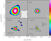 |
Fig. 1 Maps of the continuum emission from the HC H II region G24 A1 observed with the VLA at four wavelengths as indicated in each box. A logarithmic scale has been used to enhance the weakest features. The ellipse in the bottom right corner indicates the full width at half power of the synthesised beam of each map (see also Table 1). The black contours in the bottom right panel correspond to the 4σ level of the ALMA 1.4 mm map of Cesaroni et al. (2017) and M2018. The corresponding beam is shown in the bottom left of the panel. White contour levels range from 0.9 to 1.98 in steps of 0.36 mJy beam−1 at 20 cm, from 0.85 to 8.5 in steps of 2.55 mJy beam−1 at 6 cm, from 0.17 to 13.77 in steps of 3.4 mJy beam−1 at 3.6 cm, and from 0.115 to 13.915 in steps of 4.6 mJy beam−1 at 1.3 cm. In all cases, the minimum contour level corresponds to 5σ. |
2 Observations
In this section, we describe our observations of G24 A1 performed with the VLA, the IRAM/Plateau de Bure Interferometer, and the e-MERLIN. We also make use of already published ALMA data, whose observations are described in Cesaroni et al. (2017) and M2018.
We notethat in all cases the final maps presented in this article have been corrected for the apparent motion of the G24.78+0.08 region (2.6 mas yr−1 towards the west, 5.0 mas yr−1 towards the south), obtained by Moscadelli et al. (2007) by measuring the proper motions of the methanol masers associated with the hot molecular core A1N enshrouding the HC H II region A1 (see Fig. 1). The arbitrary reference date for this correction is September 20, 2015.
2.1 Very Large Array
We used the VLA to image the continuum emission from G24 A1 at various wavelengths. We also observed the H63α (at 25 686.28 MHz), H66α (at 22 364.17 MHz), and H68α (at 20 461.77 MHz) recombination lines. In all cases, the phase centre of the observations was set at the coordinates α(J2000) = 18h 36m 12. s66, δ(J2000) = −07° 12′ 10.′′15. We summarise the main characteristics of the observations in Table 1. The data reduction was made through standard procedures in the Astronomical Image Processing System (AIPS) of the National Radio Astronomy Observatory (NRAO) for all projects except 15A–019, for which we used the Common Astronomy Software Applications (CASA; McMullin et al. 2007). Further details on project 15A–019 can be found in M2018.
Since the H II region emission is sufficiently strong, in most cases the data have been self-calibrated. In order to filter out the extended emission present at the longest wavelengths, we excluded all data inside a u, v radius of 30 kλ at L band and 50 kλ at C band. When RRLs were observed (H66α in project AG732 and H63α and H68α in project 15A–019), the line data were obtained by subtracting the continuum in the u, v domain using line-free channels.
2.2 e-MERLIN
G24 A1 was observed with the e-MERLIN synthesis telescope during its cycle 0 in July 2012 (project 12A-032). The e-MERLIN array consists of seven antennas including the 76 m Lovell telescope, the 32 m dish at Cambridge, and five 25 m dish antennas distributed over the United Kingdom. The array reaches baselines up to 217 km, connected by an optical fibre network to the Jodrell Bank Observatory. The achieved angular resolution is60 mas in the C radio-frequency band of 5 GHz. We set the phase centre of the observations at α(J2000) = 18h36m12. s660, δ(J2000) = −07°12′10.′′146. The absolute flux scale was calibrated using the quasar 3C286 (1331+305) with a flux of 6.8 Jy. Gain and amplitude were corrected using the quasar 1846−0651 with a bootstrapped flux of 0.65 Jy. The bandpass response of the covered 512 MHz band was calibrated observing the bright quasar 1407+284, for which we derived a flux density of 2.287 Jy at 5.49 GHz, and a spectral index of − 0.61.
Data were reduced and analysed using AIPS. We followed the standard procedures for e-MERLIN data reduction. The calibrated visibilities of G24 A1 were imagedusing the IMAGR task of AIPS using multi-scale cleaning. We performed self-calibration to the data which marginally improved the final rms noise level down to 0.13 mJy beam−1, for a 60 mas synthesised beam.
2.3 IRAM/Plateau de Bure
We observedthe continuum and H41α recombination line at 92034.47 MHz towards G24 A1 with the interferometer on November 25, 2012. The array consisted of six elements laid out in a C configuration. The receivers were tuned at a frequency of 92.1 GHz. The bandpass and phase calibrator was 1749+096, while flux calibration was performed by means of observations of MWC349. The observations were performed with an on-source integration time of 180 min. Data calibration and imaging were made through standard procedures, using the GILDAS package1.
Maps were made with uniform weighting, with a synthesised beam with full width at half power of 3.′′ 75 × 3.′′75. The continuum maps were obtained by visually inspecting the data cubes and selecting channels with no evidence of line emission. These channels were then averaged in the u, v domain and pure continuum images were made from the averaged u, v data. The resulting continuum bandwidth was 56 MHz and the thermal noise level was 2 mJy beam−1. Line maps were obtained by subtracting the continuum data in the u, v domain. Self-calibration was performed using the line-free continuum emission. The self-calibration solutions were then applied to all the data. The resulting data cubes have a typical noise of 11 mJy beam−1 in a 0.5 km s−1 channel. Flux calibration is accurate to within 20% at both wavelengths.
Parameters of VLA observations.
3 Results
3.1 Continuum emission
In Fig. 1, we show our new VLA continuum maps of G24 A1 at 20, 6, 3.6, and 1.3 cm. Except the 6 cm image, which was obtained with the AB configuration, all the others were acquired with the A configuration of the array. The HC H II region looks basically unresolved at the two longest wavelengths, whereas a slightly elongated head-tail structure is visible at 3.6 and 1.3 cm. On the 1.3 cm map we also overlay the 4σ contour level of the 1.4 mm continuum map of Cesaroni et al. (2017) and M2018, and indicate the molecular, dusty cores identified byBeltrán et al. (2011) and M2018, using their nomenclature. We note that core A1N contains the HC H II region.
To the north-west of the HC H II region, two faint point-like sources are detected at 3.6 and 1.3 cm, both coinciding with core A2. Of the two sources, the one to the south was detected for the first time by Vig et al. (2008) with approximately twice much flux as we measured (~0.5 mJy). For the other source, we measure a flux of ~0.5 mJy, corresponding to ~ 5σ on the map of Vig et al. (2008), but these authors did not detect it. These results suggest that the two faint sources are variable, perhaps associated with shock-ionised material along the SE–NW jet/outflow imaged by Furuya et al. (2002), Beltrán et al. (2011), and Codella et al. (2013).
As noted by Beltrán et al. (2007) and confirmed by M2018, the spectral energy distribution (SED) of G24 A1 from the centimetre to the millimetre regime closely resembles that of a classical homogenous H II region, rising as ν2 in the optically thick part at long wavelengths, and flattening with flux density ∝ ν−0.1 when the emissionbecomes optically thin at high frequencies. This is shown in Fig. 2, where we plot the total flux densities integrated over the source, obtained from our data and other high-resolution data from the literature. These flux densitiesarealso given in Table 2 with the corresponding angular resolution, instrument, and reference. We note that the continuum flux density of 0.155 Jy measured by us at 92 GHz (see Sect. 2.3) in a 4.′′ 35×2.′′74 beam is not included in the table because it is significantly affected by dust emission from the surrounding molecular core, due to the beam being much greater than the angular size of the HC H II region. Therefore, this value is to be taken as an upper limit to the free-free emission and will not be considered in the following.
Beltrán et al. (2007) used the VLA in the most extended configuration complemented by the Pie Town antenna to observe G24 A1 with the best possible resolution at 1.3 cm and 7 mm. With a 56 mas beam at 7 mm, they could resolve the H II region and concluded that the emission was mostly arising from a thin shell. Our new e-MERLIN image at 5 cm with similar resolution (~60 mas) nicely complements the 7 mm image as the free–free opacity is ~70 times higher in the former than in the latter. Therefore, a comparison between the two maps can provide us with information on the internal structure of the HC H II region.
This comparison is made in Fig. 3a, where the 7 mm map of Beltrán et al. (2007) is overlaid on our e-MERLIN map. The most noticeable feature is the clear shift between the two images. Not only is the peak of the 5 cm emission offset by ~0.′′2 to the south-west of the 7 mm peak, but the 5 cm emission as a whole also appears to trace the fainter tail of the 7 mm emission and is basically undetected towards the bright north-eastern rim visible at 7 mm. We note that the observed offset between the 5 cm and 7 mm maps is not due to a positional error because the 6 cm map obtained with the VLA appears to perfectly match the e-MERLIN map despite the worse angular resolution (see Fig. 3b).
An interesting feature of the 7 mm map is the presence of a bright rim to the NE. Noticeably, the 5 cm emission appears to decrease just at the same location. The different behaviour of the emission at the two wavelengths could be ascribed to the different opacity, which is known to scale as ν−2.1. We investigate this issue in Sect. 4.3; the comparison between the two images is used to obtain information on the physical structure of the H II region.
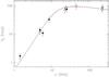 |
Fig. 2 Spectrum of the continuum emission from the HC H II region G24 A1. The points represent the measurements from our data (solid circles) and previously published data (empty circles), listed in Table 2. The error bars take into account both the errors given in the table and a conservative calibration uncertainty of 20%. The solid curve is the best fit to the data obtained for a spherical H II region, while the dashed curve is the best fit for a shell H II region with an inner radius 99% of the outer radius (see Sect. 4.1 for details on the model fit). |
Flux densities obtained by integrating the emission over the HC H II region G24 A1.
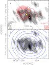 |
Fig. 3 Panel a: contour map of the 7 mm continuum emission from Beltrán et al. (2007) overlaid on our grey-scale image of the e-MERLIN map obtained at 5 cm. Contour levels range from 0.93 (=3σ) to 10.23 in steps of 1.55 mJy beam−1, while grey-scale levels range from 156 (=2σ) to 468 in steps of 78 μJy beam−1. The synthesised beams of the two maps (0.′′56 × 0.′′56 for the VLA and 0.′′097 × 0.′′038 with PA = 21° for the e-MERLIN image) are shown in the bottom left and right corners. The white dots denote the positions of the emission peaks at (from NE to SW) 7 mm, 1.3 cm, 3.6 cm, and 5 cm, while the dashed line is the best fit to these peaks. The star symbol indicates the estimated position of the star ionising the H II region (see Sect. 4.3). Panel b: same as upper panel, with a contour map of the 6 cm continuum emission imaged with the VLA. Contour levels range from 0.51 (=3σ) to 10.03 in steps of 1.3 mJy beam−1. The synthesised beam of the VLA image is 0.′′415 × 0.′′38 with PA = –16°. |
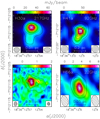 |
Fig. 4 Images of the integrated emission of the four recombination lines observed by us (colour scales) with overlaid contour maps of the continuum emission at the same frequencies. The cross indicates the peak of the H30α emission and helps comparison among the different panels. The synthesised beams of the RRL images are shown in the bottom left corners, those of the continuum maps in the bottom right corners. Contour levels range from 2.5 to 34.5 in steps of 3.4 mJy beam−1 at 217 GHz, from 10 to 154 in steps of 16 mJy beam−1 at 92 GHz, from 0.06 to 16.26 in steps of 1.8 mJy beam−1 at 25 GHz, and from 4.6 to 78.2 in steps of 9.2 mJy beam−1 at 22 GHz. In all cases, the minimum contour level corresponds to 5σ. |
3.2 Radio recombination lines
The new data presented in our study consist of four RRLs: H41α, H63α, H66α, and H68α. We also take advantage of previous observations of the H30α line, from M2018, and the H35α line, which belongs to the dataset of Furuya et al. (2002) and Cesaroni et al. (2003), although it is not explicitly mentioned in these articles.
In Fig. 4, the RRL emission is compared to the corresponding continuum emission at the same frequency. We do not show maps of the H35α and H68α lines because the former is heavily blended with other transitions of molecular species and the latter is toofaint. In all cases the RRL emission looks quite compact, even when observed with ≲0.′′2 resolution. Although the shape is very similar to the continuum emission, the latter appears to peak slightly more to the north-east of the H63α and H66α RRL peaks, possibly due to opacity effects.
In Table 3, we give the parameters of the RRLs obtained with Gaussian fits to the line profiles towards the peak of the emission. No fit was attempted to the H35α and H68α for the reasons explained above.
An interesting feature of the RRLs from G24 A1 is their broad line width (Sewilo et al. 2004). As for most HC H II regions, in this object the contribution of thermal and pressure broadening is insufficient to explain the observed line full width at half maximum (FWHM). In fact, from Eqs. (4.7) and (4.8) of Brocklehurst & Seaton (1972) we find, for example, that the pressure broadening is negligible (~0.06 km s−1) for the H30α line, even for densities as high as 106 cm−3, and for a typical electron temperature of 104 K the thermal FWHM is ~21 km s−1, significantly less than the value reported in Table 3. Therefore, a substantial contribution by large-scale motions is required. Indeed, by comparing the proper motions of the water masers surrounding the H II region to the shape of the free–free continuum emission, Moscadelli et al. (2007) and Beltrán et al. (2007) conclude that the ionised gas is confined in a shell expanding at high speed (~40 km s−1). A similar conclusion is reached by M2018, who determine a large velocity gradient through the H II region, directed approximately NE–SW and spanning ~60 km s−1. They interpret this gradient as the result of expansion of the ionised gas in a weakly collimated outflow. In Sect. 4.2, we demonstrate that an expanding shell-like H II region can indeed fit the observed profiles of the RRLs.
Integrated intensity, peak velocity, and full width at half maximum of RRLs, observed towards the peak of the emission in G24 A1.
4 Analysis and discussion
The purpose of our study is to derive the physical parameters of the H II region and determine its geometrical and kinematical structure bycombining the continuum and line data illustrated in the previous section. Based on the results of Beltrán et al. (2007), in the following we assume that the H II region is spherically symmetric and consists of a shell with inner radius Ri and outer radius Ro.
4.1 SED fit and stellar Lyman continuum
From the SED of the continuum emission we can derive a number of important quantities. The flux density of the free-free continuum emitted by a homogeneous, ionised, spherically symmetric shell is given by the following expression (see Appendix A for the derivation):
![\begin{eqnarray*} S_{\nu} & = & B_{\nu}(T_{\textrm{e}}) \, \frac{\pi\,R_{\textrm{o}}^2}{d^2} \nonumber \\ & & \times \left[ 1+\frac{2}{\tau_{\textrm{o}}} \left(\sqrt{1-r_{\textrm{i}}^2} \, {e}^{-\tau_{\textrm{o}}\sqrt{1-r_{\textrm{i}}^2}} + \frac{{e}^{-\tau_{\textrm{o}}\sqrt{1-r_{\textrm{i}}^2}}-1}{\tau_{\textrm{o}}}\right) \right.\\ & & \left. - \int_0^{r_{\textrm{i}}^2} { e}^{-\tau_{\textrm{o}}\left(\sqrt{1-x}-\sqrt{r_{\textrm{i}}^2-x}\right)} \textrm{d}x \right], \nonumber \end{eqnarray*}](/articles/aa/full_html/2019/04/aa34700-18/aa34700-18-eq1.png) (1)
(1)
where d is the source distance, Bν is the Planck function, Te is the electron temperature, ri = Ri∕Ro, and τo is the free-free opacity corresponding to a geometrical path 2Ro. The last is computed from Eq. (A-1a) of Mezger & Henderson (1967). In the optically thick and thin limits Eq. (1) takes the form

The balance between ionisations and recombinations in a shell H II region under the “on-the-spot” approximation (see e.g. Spitzer 1998) is given by the relation
 (4)
(4)
where ne is the electron density,  cm3 s−1 the recombination coefficient of a hydrogen plasma excluding recombinations to the ground state, and NLy is the number of Lyman continuum photons emitted by the star per unit time.
Using all these equations, it is possible to express Sν as a function of ν, Te, Ro, ri, NLy, and d and fit the SED in Fig. 2. Before searching for the best fit, it is worth minimising the numberof free parameters. The distance is fixed to 6.7 kpc. Moreover, although some temperature gradients could be present inside the H II region, it seems reasonable to assume that the bulk of the ionised gas has Te = 104 K. Finally, we argue that the flux density is very weakly dependent on ri. This can be seen in the optically thick and thin limits. Equation (2) is obviously independent of ri. Moreover, since  , from Eq. (4) we obtain
 ![$\tau_{\textrm{o}}\propto N_{\textrm{Ly}}/[{R_{\textrm{o}}}^2(1-{r_{\textrm{i}}}^3)]$](/articles/aa/full_html/2019/04/aa34700-18/aa34700-18-eq6.png) . This implies that Sν from Eq. (3) is also independent of ri.
. This implies that Sν from Eq. (3) is also independent of ri.
With this in mind, in the following we consider two extreme cases with ri = 0 and ri = 0.99, to confirm the expectation that the fit is basically insensitive to the value of ri. Assuming ri = 0, we are left with only two free parameters in Eq. (1): Ro and NLy. In order to determine the best fit, we minimise the χ2 by varying these parameters over the ranges shown in Fig. 5. The minimum χ2 is attained for Ro = 0.153 arcsec (i.e. 1025
 au) and NLy = (5.3 ± 0.7) × 1047 s−1, corresponding to an O9.5 zero age main sequence star (Panagia 1973). The best fit is shown by the solid curve in Fig. 2. The value of Ro compares nicely with the size of the head–tail structure observed in the continuum images of G24 A1 (see e.g. Fig. 3a), which confirms the goodness of the fit.
We repeated the procedure, this time assuming ri = 0.99 and obtained the same best-fit parameters, as expected. The corresponding fit is represented by the red dashed curve in Fig. 2, which is in practice indistinguishable from the previous fit.
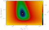 |
Fig. 5 Plot of χ2 obtained by fitting Eq. (1) to the data in Table 2. The minimum is marked by the white dot, while the contours correspond to 68% (1σ) and 99% reliability (see Table 1 in Lampton et al. 1976) and the corresponding levels are indicated in the colour scale to the right. |
4.2 Structure and density of the HC H II region
In the previous section, we show that the fit to the SED of a shell H II region is basically independent of ri. Therefore, we cannot obtain any morphological information nor do we know the value of the electron density. From Eq. (4) it is clear that ne is very sensitive to the thickness of the shell. It is thus important to obtain a reliable value of ri. Beltrán et al. (2007) estimated ri directly from the high-resolution map at 7 mm, obtaining ri ≃ 0.9. Here, we use a different approach, based on the RRL information.
The intensity and shape of RRLs provide us with a wealth of information on the physical parameters and velocity structure of the ionised gas. In particular, in the case of G24 A1 we want to establish whether the H II region is indeed expanding at high speed, as suggested by the H2O maser proper motions Moscadelli et al. (2007). For this purpose we have developed a numerical model that calculates the intensity of an RRL emerging from a homogenous shell H II region, expanding with constant radial velocity vo. The model solves the radiative transfer equation along a generic line of sight through the shell H II region, assuming constant electron density and temperature. The absorption and emission coefficients are obtained from Eqs. (3.19) and (3.25) of Brocklehurst & Seaton (1972). Non-LTE effects are taken into account using the program code in Appendix E of Gordon & Sorochenko (2002) to compute the departure coefficients that appear in Eqs. (3.13) and (3.14) of Brocklehurst & Seaton (1972). The coefficients are calculated for given electron temperature and density, assuming case B recombination. Although some asymmetry is visible in the continuum and line maps of Figs. 1 and 4, our assumption of spherical symmetry is sufficient for our purposes given the limited angular resolution of the RRL observations.
The input parameters of our model are Te, Ro, ri, ne, vo, and d. For G24 A1 we know that d = 6.7 kpc. For a given RRL, the model computes the line profile towards the centre of the H II region as a function of velocity (or frequency). The result is also convolved with a Gaussian beam to allow comparison with the observed spectrum. In the case of G24 A1 we decided to fit only three out of the six RRLs available, those with little or no contamination from molecular lines and with a good signal-to-noise ratio (S/N), namely the H30α, H41α, and H66α lines, which were all smoothed to the coarsest spectral resolution (~3.2 km s−1) before searching for the best fit. The best fit was obtained by minimising the expression
 (5)
(5)
where indices i and k respectively denote the recombination line and the spectral channel, ni and σi the number of channels and the noise of spectrum i, Vk the velocity of channel k,  the brightness temperature computed with our model at velocity Vk, and
  the measured brightness temperatureof spectrum i at channel k. We note that σi includes both thermal noise and the calibration error (20%) which are summed in quadrature. A systemic local standard of rest velocity VLSR = 112 km s−1 is summed to the velocity of the model spectra before computing the value of χ2.
To minimise the number of free parameters, we assume Te = 104 K and express ne as a function of Ro and Ri by means of Eq. (4), after fixing NLy = 5.3 × 1047 s−1 (see Sect. 4.1). For the line profile we assume a Voigt function, which contains both Doppler and pressure broadening, as described in Sect. 4 of Brocklehurst & Seaton (1972). Following their approach, we also take into account a contribution to the Doppler line width by turbulence, by introducing a “Doppler temperature” (see their Eq. (4.3)). In practice, this means that to the normal thermal broadening of the line of 21.5 km s−1 (corresponding to Te = 104 K) we sum in quadrature an additional line width due to turbulent broadening. This is assumed equal to the typical FWHM of the molecular transitions from the hot core enshrouding the H II region, i.e. ~7 km s−1 (see e.g. Beltrán et al. 2005), corresponding to ~1000 K. In conclusion, we assume a Doppler temperature of 11 000 K.
The minimum value of χ2 was searched for by varying Ro, ri, and vo over suitable ranges, as illustrated in Fig. 6. The best fit is shown in Fig. 7 and corresponds to Ro =  arcsec (i.e.
  au), ri =
  , and vo = 16 ± 4 km s−1. We note that the fitted spectra are those on the left side of the figure. The three spectra on the right side are shown for the sake of comparison with the model predictions, but were not used to compute the χ2 and hence constrain the fit.
While the best-fit model reproduces the intensities and widths of all RRLs quite well, there is some discrepancy in the line shape for the H63α and H68α lines. Both the observed and model profiles are slightly skewed to blue-shifted velocities (due to the interplay between expansion and opacity of the ionised gas), but the former seems to peak at lower velocities than the latter. This difference could be due to the asymmetry of the HC H II region due to its head–tail structure, which is not considered in our spherically symmetric model. The H63α and H68α lines are those observed with the smallest beams, which barely resolve the H II region. However, given the poor S/N of the two spectra we prefer not to speculate further on this issue.
The size obtained from the fit to the RRLs differs by ~30% from the value computed from the fit to the SED (see Sect. 4.1). This is not surprising because the RRL emission appears slightly more compact than the continuum emission, as can be seen in Fig. 4. This difference is probably due to the different S/N of the two datasets.
An important result of our fits is that the value of ri is consistent with the findings of Beltrán et al. (2007), confirming that G24 A1 consists of a thin shell ofionised gas. The density of such a shell can be estimated from Eq. (4) as ne =  cm−3.
cm−3.
A few considerations are in order on the expansion velocity. The mere fact that the ionised gas is expanding indicates that the H II region is not gravitationally trapped. According to Keto (2007) the critical radius below which the H II region is confined is given by his Eq. (3) and is ~50 au, much less than our estimation of 780 au. Moreover, vo ≃16 km s−1 is in good agreement with the H II region undergoing expansion at the sound speed in the ionised gas, which is ~13 km s−1. These values are at variance with the expansion velocity of ~40 km s−1 derived from the water maser proper motion measurements by Moscadelli et al. (2007) and Beltrán et al. (2007). This is about twice as high as the value we obtained for vo. This discrepancy suggests that the velocities of the H2O maser spotscould consist of two components, one due to the expansion of the H II region (vo), the other to the translational motion of the star and associated ionised gas across the molecular cloud. In turn, this implies that the expansion timescale of the HC H II region should be about twice that predicted by Beltrán et al. (2007), namely ~50–150 yr.
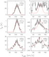 |
Fig. 7 Spectra of the RRLs observed towards G24 A1 (histograms) compared to the best-fit model (red curves). Only the three lines to the left have been used to constrain the fit; those to the right are shown for the sake of comparison with the model predictions. The shaded area indicates the calibration uncertainty (20%). The line name and the corresponding angular resolution are given in the top right corner of each box. |
4.3 The vanishing bright rim
An intriguing feature of the continuum maps of G24 A1 is that the bright rim to the NE appearing in the 7 mm map is not detected at all at 5 cm (see Fig. 3). It is very likely that opacity effects play a crucial role in this context. In fact, the peak of the continuum emission progressively shifts away from the 7 mm bright rim towards the 5 cm peak (i.e. from NE to SW) as the observing frequency decreases and the free–free continuum optical depth grows. This is shown in Fig. 3a, where the peak positions at 7 mm, 1.3 cm, 3.6 cm, and 5 cm are indicated by the white dots. We adopt a straight line, obtained as the best fit passing through these peaks (also indicated in Fig. 3a) as the symmetry axis of the head-tail structure. This line is perfectly consistent with the direction defined by the H30α velocity gradient derived by M2018 (see the dashed line in their Fig. 9).
Figure 8 shows the brightness temperature profiles at 7 mm and 5 cm along this axis. The presence of the bright rim at 7 mm and its absence at 5 cm are evident in this plot. In the following, we demonstrate that all of this cannot be explained with a simple model of a homogeneous shell H II region, but a combination of a temperature gradient and opacity effects is needed.
In order to demonstrate that this is the case, we slightly modified our model of a spherically symmetric shell H II region. We divided the shell into two parts with different Te, separated atradius Rl, namely:
![\begin{eqnarray*} T_{\textrm{e}}(R) & = & \left\{ \begin{array}{lcl} 10^4~\textrm{K} & \Leftrightarrow & R_{\textrm{i}} \le R < R_{\textrm{l}} \\[4pt] 3\times10^3~\textrm{K} & \Leftrightarrow & R_{\textrm{l}} \le R < R_{\textrm{o}}.\end{array} \right. \end{eqnarray*}](/articles/aa/full_html/2019/04/aa34700-18/aa34700-18-eq16.png) (6)
(6)
This is a simple way to parametrise the temperature drop at the border of H II regions predicted by numerical calculations (see e.g. Evans 1991). The temperature in the outer layer was arbitrarily chosen as equal to 3000 K because this is consistent with the mean value of the brightness temperature measured at the optically thick frequency of 5 GHz (see Fig. 8).
We then computed the brightness temperature profile along a radial direction at both 7 mm and 5 cm. The input parameters of the model for a given frequency are Ro, ne, ri, Rl ∕Ro, and d. Moreover, since we do not know the position of the star, we also introduced an unknown positional offset along the cut to be added to the radial profile computed by the model. For G24 A1 we have d = 6.7 kpc and, from our fit to the RRLs, we can also fix Ro = 0.′′116 and ri = 0.89. We are thus left with three free parameters: ne, Rl ∕Ro, and the positional offset.
The χ2 was computed from the difference between the observed profiles and the model profiles, after convolving the latter with the instrumental beams. The minimum χ2 was determined by varying the free parameters over the ranges shown in Fig. 9. The minimum is attained for ne =  cm−3, Rl ∕Ro = 0.989
 , and an offset of 0.′′0313 ± 0.′′ 006 corresponding to the position α(J2000) = 18h 36m 12. s5511, δ(J2000) = −07° 12′ 10.′′883, marked by the starred symbol in Fig. 3a.
The top panel of Fig. 9 demonstrates that an H II region with constant Te cannot fit the data, because for Rl∕Ro = 1 the value of χ2 lies well above the 99% confidence level, whatever the offset. This clearly shows that a low-temperature layer is needed toexplain the observed brightness profiles. Indeed, the best-fit profiles agree quite well with the data within the noise, as shown in Fig. 8. We conclude that the electron temperature in a thin layer at the surface of the H II region G24 A1 is significantly lower than the typical value of ~ 104 K.
Finally, we note that the best-fit value of ne is greater than that obtained in Sect. 4.2 (~ 7 × 105 cm−3) because we fit the brightness profile along the radial direction corresponding to the maximum brightness temperature and at the same time assumed a spherically symmetric model. The overall brightness of the model is thus greater than the observed value, which turns into an overestimate of ne with respectto the value obtained from integrated quantities over the whole HC H II region (see Sects. 4.1 and 4.2).
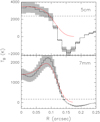 |
Fig. 8 Brightness temperature profiles of the continuum emission from G24 A1 at 7 mm and 5 cm obtained along the dashed line in Fig. 3a. Variable R is the angular distance from the star, which hence lies at R = 0 in our model (see text). The dashed horizontal lines denote the 3σ noise levels at the two wavelengths. The red curves are the best fit to the data. |
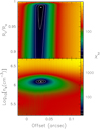 |
Fig. 9 Plot of χ2 for the difference between the data profiles in Fig. 8 and the profiles computed with the model described in the text. The free variables are the offset identifying the position of the star, the ratio Rl ∕Ro, and the electron density. The white dots and contour levels have the same meaning as in Fig. 5. |
5 Summary and conclusions
We have performed interferometric observations of the continuum and hydrogen recombination lines towards the HC H II region G24 A1. By complementing our new data with results from the literature, we have presented an analysis of the structure and kinematics of the ionised gas. We show that the H II region, which is shaped like a comet, can be successfully approximated with an expanding shell despite the presence of a tail of ionised gas towards SW. We have developed a simple model assuming such a shell structure and could fit both the free–free continuum and RRL emission deriving a number of physical parameters. In particular, we estimate a radius of 780–1030 au, a shell thickness ~90% of the radius, an expansion speed of ~16 km s−1, a stellar Lyman continuum of 5.3 × 1047 s−1 corresponding to an O9.5 star, and an electron density of ~ 106 cm−3. With respect to the previous findings of Beltrán et al. (2007), our results not only improve on the accuracy of the derived parameters, but also demonstrate that the HC H II region is expanding at about half the speed previously estimated. We conclude that G24 A1 is a young H II region which is both undergoing expansion and drifting inside the parental molecular core. Moreover, for the first time we find evidence of a sharp temperature gradient in the ionised gas of G24 A1, indicating a significant drop of the electron temperature (down to a few 1000 K) in a thin layer at the outer border of the shell H II region.
Acknowledgements
We express our appreciation to our late friend and colleague Malcolm Walmsley for all the stimulating discussions and his advice on the physics of RRLs, which have been crucial for the development of the model presented in this article. A.S.M. is thankful to Pierre-Emmanuel Belles for his support on the calibration and data reduction of the eMERLIN data. We thank the Italian ARC node and the IRAM technical staff for their support for this project. A.S.M. acknowledges support from the Deutsche Forschungsgemeinschaft (DFG) via the Sonderforschungsbereich SFB 956 (project A6). The research leading to these results has received funding from the European Unions Horizon 2020 research and innovation programme under grant agreement No 730562 [RadioNet]. e-MERLIN is a National Facility operated by the University of Manchester at Jodrell Bank Observatory on behalf of STFC. This study is based on observations made under projects AG732, AB1300, AB1278, AB1246, 15A–019 of the VLA of NRAO. The National Radio Astronomy Observatory is a facility of the National Science Foundation operated under cooperative agreement by Associated Universities, Inc. This work is also based on observations carried out under project number W072 with the IRAM interferometer. IRAM is supported by INSU/CNRS (France), MPG (Germany), and IGN (Spain).
Appendix A Flux density from a shell
In the following, we derive the expression of the flux density from a spherical, homogenous, isothermal shell in LTE, with outer radius Ro and inner radius Ri (see sketch in Fig. A.1).
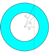 |
Fig. A.1 Sketch of shell with inner and outer radii Ri and Ro, respectively. The dashed line indicates a generic line of sight with impact parameter R. |
The total flux density from the shell, Sν, is obtained by integrating the brightness over the solid angle 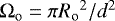 subtended by the shell, namely over all lines of sight crossing the shell
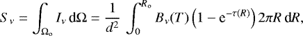 (A.1)
(A.1)
where Bν is the Planck function, T the gas temperature, d the source distance, and τ the opacity along a generic line of sight with impact parameter R. The optical depth can be expressed as
 (A.2)
(A.2)
where we have defined r = R∕Ro, ri = Ri∕Ro, and τo is the opacity corresponding to a geometrical path 2Ro.
Equation (A.1) can now be rewritten as
![\begin{eqnarray*} S_{\nu} & = & B_{\nu}(T) \, \frac{\pi{R_{\textrm{o}}}^2}{d^2} \times \left\{ \int_0^1 2 r \, \textrm{d}r \right. \nonumber\\ & & - \int_{{r_{\textrm{i}}}}^1 \exp\left(-{\tau_{\textrm{o}}}\sqrt{1-r^2}\right) 2 r \, \textrm{d}r \nonumber\\ & & \left. - \int_0^{{r_{\textrm{i}}}} \exp\left[-{\tau_{\textrm{o}}}\left(\sqrt{1-r^2}-\sqrt{r_{\textrm{i}}^2-r^2}\right)\right] 2 r \, \textrm{d}r \right\}. \end{eqnarray*}](/articles/aa/full_html/2019/04/aa34700-18/aa34700-18-eq22.png) (A.3)
(A.3)
From this, defining x = r2, we eventually obtain
![\begin{eqnarray*} S_{\nu} & = & B_{\nu}(T) \, \frac{\pi\,R_{\textrm{o}}^2}{d^2} \nonumber \\ & & \times \left[ 1+\frac{2}{\tau_{\textrm{o}}} \left(\sqrt{1-r_{\textrm{i}}^2} \, {e}^{-\tau_{\textrm{o}}\sqrt{1-r_{\textrm{i}}^2}} + \frac{{e}^{-\tau_{\textrm{o}}\sqrt{1-r_{\textrm{i}}^2}}-1}{\tau_{\textrm{o}}}\right) \right. \\ & & \left. - \int_0^{r_{\textrm{i}}^2} \textrm{e}^{-\tau_{\textrm{o}}\left(\sqrt{1-x}-\sqrt{r_{\textrm{i}}^2-x}\right)} \textrm{d}x \right]. \nonumber \end{eqnarray*}](/articles/aa/full_html/2019/04/aa34700-18/aa34700-18-eq23.png) (A.4)
(A.4)
References
- Beltrán, M. T., Cesaroni, R., Neri, R., et al. 2005, A&A, 435, 901 [NASA ADS] [CrossRef] [EDP Sciences] [Google Scholar]
- Beltrán, M. T., Cesaroni, R., Moscadelli, L., & Codella, C. 2007, A&A, 471, L13 [NASA ADS] [CrossRef] [EDP Sciences] [Google Scholar]
- Beltrán, M. T., Cesaroni, R., Zhang, Q., et al. 2011, A&A, 532, A9 [NASA ADS] [CrossRef] [EDP Sciences] [Google Scholar]
- Brocklehurst, M., & Seaton, M. J. 1972, MNRAS, 157, 179 [NASA ADS] [CrossRef] [Google Scholar]
- Cesaroni, R., Codella, C., Furuya, R. S., & Testi, L. 2003, A&A, 549, A146 [Google Scholar]
- Cesaroni, R., Sánchez-Monge, Á., Beltrán, M. T., et al. 2017, A&A, 602, A59 [NASA ADS] [CrossRef] [EDP Sciences] [Google Scholar]
- Codella, C., Testi, L., & Cesaroni, R. 1997, A&A, 325, 282 [NASA ADS] [Google Scholar]
- Codella, C., Beltrán, M. T., Cesaroni, R., et al. 2013, A&A, 550, A81 [NASA ADS] [CrossRef] [EDP Sciences] [Google Scholar]
- Evans, I. N. 1991, ApJS, 76, 985 [NASA ADS] [CrossRef] [Google Scholar]
- Furuya, R. S., Cesaroni, R., Codella, C., et al. 2002, A&A, 390, L1 [NASA ADS] [CrossRef] [EDP Sciences] [Google Scholar]
- Galván-Madrid, R., Peters, T., Keto, E., et al. 2011, MNRAS, 416, 1033 [NASA ADS] [CrossRef] [Google Scholar]
- Gordon, M. A., & Sorochenko, R. L. 2002, Radio Recombination Lines: Their Physics and Astronomical Applications, Astrophysics and Space Science Library (The Netherlands: Springer), 282 [Google Scholar]
- Hoare, M. G., Purcell, C. R., Churchwell, E. B., et al. 2012, PASP, 124, 939 [NASA ADS] [CrossRef] [Google Scholar]
- Keto, E. 2007, A&A, 666, 976 [Google Scholar]
- Klaassen, P. D., Johnston, K. G., Urquhart, J. S., et al. 2018, A&A, 611, A99 [NASA ADS] [CrossRef] [EDP Sciences] [Google Scholar]
- Kurtz, S. 2005, IAU Symp., 227, 111 [NASA ADS] [CrossRef] [Google Scholar]
- Lampton, M., Margon, B., & Bowyer, S. 1976, ApJ, 208, 177 [NASA ADS] [CrossRef] [Google Scholar]
- McMullin, J. P., Waters, B., Schiebel, D., Young, W., & Golap, K. 2007, ASP Conf. Ser., 376, 127 [Google Scholar]
- Mezger, P. G.,& Henderson, A. P. 1967, ApJ, 147, 471 [NASA ADS] [CrossRef] [Google Scholar]
- Moscadelli, L., Goddi, C., Cesaroni, R., Beltrán, M. T., & Furuya, R. 2007, A&A, 472, 867 [NASA ADS] [CrossRef] [EDP Sciences] [Google Scholar]
- Moscadelli, L., Rivilla, V. M., Cesaroni, R., et al. 2018, A&A, 616, A66 [NASA ADS] [CrossRef] [EDP Sciences] [Google Scholar]
- Panagia, N. 1973, AJ, 78, 929 [NASA ADS] [CrossRef] [Google Scholar]
- Peters, T., Banerjee, R., Klessen, R. S., et al. 2010, ApJ, 711, 1017 [NASA ADS] [CrossRef] [Google Scholar]
- Purcell, C. R., Hoare, M. G., Cotton, W. D., et al. 2013, ApJS, 205, 1 [NASA ADS] [CrossRef] [Google Scholar]
- Sewilo, M., Churchwell, E., Kurtz, S., Goss, W. M., & Hofner, P. 2004, ApJ, 605, 285 [NASA ADS] [CrossRef] [Google Scholar]
- Sollins, P. K., Zhang, Q., Keto, E., & Ho, P. T. P. 2005, ApJ, 624, L49 [NASA ADS] [CrossRef] [Google Scholar]
- Spitzer, L. 1998, Physical Processes in the Interstellar Medium (Weinheim: Wiley-VCH) [CrossRef] [Google Scholar]
- Vig, S., Cesaroni, R., Testi, L., Beltrán, M. T., & Codella, C. 2008, A&A, 488, 605 [NASA ADS] [CrossRef] [EDP Sciences] [Google Scholar]
The GILDAS software has been developed at IRAM and Observatoire de Grenoble; see http://www.iram.fr/IRAMFR/GILDAS
All Tables
Flux densities obtained by integrating the emission over the HC H II region G24 A1.
Integrated intensity, peak velocity, and full width at half maximum of RRLs, observed towards the peak of the emission in G24 A1.
All Figures
|
Fig. 1 Maps of the continuum emission from the HC H II region G24 A1 observed with the VLA at four wavelengths as indicated in each box. A logarithmic scale has been used to enhance the weakest features. The ellipse in the bottom right corner indicates the full width at half power of the synthesised beam of each map (see also Table 1). The black contours in the bottom right panel correspond to the 4σ level of the ALMA 1.4 mm map of Cesaroni et al. (2017) and M2018. The corresponding beam is shown in the bottom left of the panel. White contour levels range from 0.9 to 1.98 in steps of 0.36 mJy beam−1 at 20 cm, from 0.85 to 8.5 in steps of 2.55 mJy beam−1 at 6 cm, from 0.17 to 13.77 in steps of 3.4 mJy beam−1 at 3.6 cm, and from 0.115 to 13.915 in steps of 4.6 mJy beam−1 at 1.3 cm. In all cases, the minimum contour level corresponds to 5σ. |
| In the text | |
|
Fig. 2 Spectrum of the continuum emission from the HC H II region G24 A1. The points represent the measurements from our data (solid circles) and previously published data (empty circles), listed in Table 2. The error bars take into account both the errors given in the table and a conservative calibration uncertainty of 20%. The solid curve is the best fit to the data obtained for a spherical H II region, while the dashed curve is the best fit for a shell H II region with an inner radius 99% of the outer radius (see Sect. 4.1 for details on the model fit). |
| In the text | |
|
Fig. 3 Panel a: contour map of the 7 mm continuum emission from Beltrán et al. (2007) overlaid on our grey-scale image of the e-MERLIN map obtained at 5 cm. Contour levels range from 0.93 (=3σ) to 10.23 in steps of 1.55 mJy beam−1, while grey-scale levels range from 156 (=2σ) to 468 in steps of 78 μJy beam−1. The synthesised beams of the two maps (0.′′56 × 0.′′56 for the VLA and 0.′′097 × 0.′′038 with PA = 21° for the e-MERLIN image) are shown in the bottom left and right corners. The white dots denote the positions of the emission peaks at (from NE to SW) 7 mm, 1.3 cm, 3.6 cm, and 5 cm, while the dashed line is the best fit to these peaks. The star symbol indicates the estimated position of the star ionising the H II region (see Sect. 4.3). Panel b: same as upper panel, with a contour map of the 6 cm continuum emission imaged with the VLA. Contour levels range from 0.51 (=3σ) to 10.03 in steps of 1.3 mJy beam−1. The synthesised beam of the VLA image is 0.′′415 × 0.′′38 with PA = –16°. |
| In the text | |
|
Fig. 4 Images of the integrated emission of the four recombination lines observed by us (colour scales) with overlaid contour maps of the continuum emission at the same frequencies. The cross indicates the peak of the H30α emission and helps comparison among the different panels. The synthesised beams of the RRL images are shown in the bottom left corners, those of the continuum maps in the bottom right corners. Contour levels range from 2.5 to 34.5 in steps of 3.4 mJy beam−1 at 217 GHz, from 10 to 154 in steps of 16 mJy beam−1 at 92 GHz, from 0.06 to 16.26 in steps of 1.8 mJy beam−1 at 25 GHz, and from 4.6 to 78.2 in steps of 9.2 mJy beam−1 at 22 GHz. In all cases, the minimum contour level corresponds to 5σ. |
| In the text | |
|
Fig. 5 Plot of χ2 obtained by fitting Eq. (1) to the data in Table 2. The minimum is marked by the white dot, while the contours correspond to 68% (1σ) and 99% reliability (see Table 1 in Lampton et al. 1976) and the corresponding levels are indicated in the colour scale to the right. |
| In the text | |
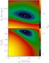 |
Fig. 6 Same as Fig. 5, but for the χ2 computed from Eq. (5) as a function of Ro, ri, and vo. |
| In the text | |
|
Fig. 7 Spectra of the RRLs observed towards G24 A1 (histograms) compared to the best-fit model (red curves). Only the three lines to the left have been used to constrain the fit; those to the right are shown for the sake of comparison with the model predictions. The shaded area indicates the calibration uncertainty (20%). The line name and the corresponding angular resolution are given in the top right corner of each box. |
| In the text | |
|
Fig. 8 Brightness temperature profiles of the continuum emission from G24 A1 at 7 mm and 5 cm obtained along the dashed line in Fig. 3a. Variable R is the angular distance from the star, which hence lies at R = 0 in our model (see text). The dashed horizontal lines denote the 3σ noise levels at the two wavelengths. The red curves are the best fit to the data. |
| In the text | |
|
Fig. 9 Plot of χ2 for the difference between the data profiles in Fig. 8 and the profiles computed with the model described in the text. The free variables are the offset identifying the position of the star, the ratio Rl ∕Ro, and the electron density. The white dots and contour levels have the same meaning as in Fig. 5. |
| In the text | |
|
Fig. A.1 Sketch of shell with inner and outer radii Ri and Ro, respectively. The dashed line indicates a generic line of sight with impact parameter R. |
| In the text | |
Current usage metrics show cumulative count of Article Views (full-text article views including HTML views, PDF and ePub downloads, according to the available data) and Abstracts Views on Vision4Press platform.
Data correspond to usage on the plateform after 2015. The current usage metrics is available 48-96 hours after online publication and is updated daily on week days.
Initial download of the metrics may take a while.