| Issue |
A&A
Volume 576, April 2015
|
|
|---|---|---|
| Article Number | A37 | |
| Number of page(s) | 16 | |
| Section | The Sun | |
| DOI | https://doi.org/10.1051/0004-6361/201323358 | |
| Published online | 24 March 2015 | |
Soft X-ray emission in kink-unstable coronal loops⋆
1
LESIA, Observatoire de Paris, CNRS, UPMC, Université
Paris-Diderot,
5 place Jules Janssen,
92195
Meudon,
France
e-mail:
rui.pinto@obspm.fr
2
Laboratoire AIM Paris-Saclay, CEA/Irfu Université Paris-Diderot
CNRS/INSU, 91191
Gif-sur-Yvette,
France
Received: 30 December 2013
Accepted: 21 January 2015
Context. Solar flares are associated with intense soft X-ray emission generated by the hot flaring plasma in coronal magnetic loops. Kink-unstable twisted flux-ropes provide a source of magnetic energy that can be released impulsively and may account for the heating of the plasma in flares.
Aims. We investigate the temporal, spectral, and spatial evolution of the properties of the thermal continuum X-ray emission produced in such kink-unstable magnetic flux-ropes and discuss the results of the simulations with respect to solar flare observations.
Methods. We computed the temporal evolution of the thermal X-ray emission in kink-unstable coronal loops based on a series of magnetohydrodynamical numerical simulations. The numerical setup consisted of a highly twisted loop embedded in a region of uniform and untwisted background coronal magnetic field. We let the kink instability develop, computed the evolution of the plasma properties in the loop (density, temperature) without accounting for mass exchange with the chromosphere. We then deduced the X-ray emission properties of the plasma during the whole flaring episode.
Results. During the initial (linear) phase of the instability, plasma heating is mostly adiabatic (as a result of compression). Ohmic diffusion takes over as the instability saturates, leading to strong and impulsive heating (up to more than 20 MK), to a quick enhancement of X-ray emission, and to the hardening of the thermal X-ray spectrum. The temperature distribution of the plasma becomes broad, with the emission measure depending strongly on temperature. Significant emission measures arise for plasma at temperatures higher than 9 MK. The magnetic flux-rope then relaxes progressively towards a lower energy state as it reconnects with the background flux. The loop plasma suffers smaller sporadic heating events, but cools down globally by thermal conduction. The total thermal X-ray emission slowly fades away during this phase, and the high-temperature component of the emission measure distribution converges to the power-law distribution EM ∝ T-4.2. The twist deduced directly from the X-ray emission patterns is considerably lower than the highest magnetic twist in the simulated flux-ropes.
Key words: Sun: corona / Sun: flares / Sun: X-rays, gamma rays
Movies associated to Figs. 4 and 5 are available in electronic form at http://www.aanda.org
© ESO, 2015
1. Introduction
Solar flares are energetic phenomena characterised by a quick enhancement of luminosity in a wide spectral range. In the soft X-ray domain, in particular, the emitting flux can increase on many orders of magnitudes on time-scales of tens of seconds to minutes (Fletcher et al. 2011). Solar flares are usually interpreted as fast releases of magnetic energy stored in the solar corona. Several energy-storage scenarios are envisioned in the literature. We consider here the scenario in which magnetic energy is stored in twisted magnetic flux-ropes in the corona. Such magnetic structures are unstable with respect to the kink mode if they are twisted above a certain threshold, whose value depends on geometrical properties specific to each individual flux-rope (such as their aspect ratio and transverse pitch angle distribution; Bareford et al. 2013). Mechanical perturbations either at their foot-points or at coronal heights may drive them out of their state of equilibrium and trigger the kink instability. Coronal loops undergoing a kink instability experience an initial linear growth phase until they start reconnecting with the background field (Browning et al. 2008). They then relax onto a lower energy state (with less twist), hence releasing a fraction of the magnetic free energy stored initially. This mechanism has been suggested to be at the origin of solar flares of different types (both confined and ejective) and at different spatial scales (from nano-flares to X class flares; Hood & Priest 1979; Linton et al. 1996; Galsgaard & Nordlund 1997; Lionello et al. 1998; Shibata & Yokoyama 1999; Török & Kliem 2005; Rappazzo et al. 2013, and references therein).
Large flares produce signatures of discrete plasma structures that are considerably hotter than the coronal background, while smaller and more frequent flares also contribute to the diffuse “background” coronal heating. The latter kind motivated many studies of coronal loop heating by multiple small amplitude impulsive heating events, such as nano-flares (Cargill & Bradshaw 2013; Bradshaw & Cargill 2013; West et al. 2008; Porter & Klimchuk 1995; Fisher & Hawley 1990; Klimchuk et al. 2008, among many others) and turbulent heating (Parenti et al. 2006; Buchlin et al. 2007; Verdini et al. 2012; van Ballegooijen et al. 2014). The majority of these studies focused on describing in detail the hydrodynamics and heat exchanges occurring in the direction parallel to the magnetic field at the expense of neglecting the transverse gradients and the effects of curvature (see, e.g., the review by Reale 2010). This strategy was initially inspired by observations of ultraviolet and X-ray emission structured into multiple thin arched structures that connect regions of opposite polarity at the surface (e.g. Vaiana et al. 1973, based on early rocket-launched missions). Improvements of this approach include models of multiple parallel one-dimensional loop strands (Reale & Peres 2000) and of groups of fine loop strands spreading throughout three-dimensional models of observed active regions (Winebarger et al. 2014), where each strand is treated as a single and independent system. These studies have been providing increasingly more sophisticated emission diagnostics, particularly in the extreme ultraviolet (EUV) range. However, this thin-thread approach is less appropriate for strong amplitude oscillations or if the loops undergo magnetic reconnection, as is the case in kink-unstable twisted loops that lead to larger flares with significant X-ray emission.
It is often pointed out that the kink-instability scenario requires very high twist in the flaring coronal loops. However, observations of flaring coronal loops most often indicate moderate twist, while highly twisted pre-flare coronal flux-ropes are indeed more rarely observed. Notable examples exist, nevertheless, such as the highly twisted flux-rope observed by Srivastava et al. (2010), which is presumably related to the occurrence of a B5.0 class flare. The total twist angle of the observed structure is of about 12π for a loop length of about 80 Mm and loop radius ≈4 Mm (placing it above the Kruskal-Shafranov twist threshold for the kink instability). Additionally, many studies of flux-rope buoyant rise and emergence suggest that highly twisted coronal loops are ubiquitous. These twisted magnetic structures are believed to be generated deep inside the solar convection zone (see e.g., Nelson et al. 2014). Under the correct circumstances, they will rise buoyantly across the turbulent convective layers and emerge into the chromosphere and the corona (Jouve & Brun 2009; Archontis & Hood 2012; Pinto & Brun 2013). Emonet & Moreno-Insertis (1998) have shown that there is a minimum amount of magnetic twist these flux-ropes must have to be able to maintain their coherence during the rise through the convection zone. Several of these works suggest that this threshold is high enough to be compatible with the kink-instability scenario. This is an important point because slow helical surface motions alone are unlikely to transmit enough twist to initially untwisted magnetic coronal structures (Hood et al. 1989; Grappin et al. 2008). The actual process of transmission of twist up to the corona remains elusive at the present date, however.
In an attempt to link magnetic twist and observations of twisted loops, Botha et al. (2012) investigated the emission properties in the EUV range of modelled straight coronal flux-ropes that undergo a kink instability by means of numerical magnetohydrodynamical (MHD) simulations. Gordovskyy & Browning (2011) studied the consequences of the reconnection driven by the onset of the kink instability on the acceleration of particles using similar MHD models and estimated the corresponding hard X-ray signature.
In this paper, we analyse the evolution of the soft X-ray continuum emission in a modelled kink-unstable coronal loop. Our aim is to investigate whether this type of models is capable of predicting the main properties of soft X-ray emission in solar flares, rather than providing exact reproductions of observations. We consider straight twisted magnetic flux ropes that are already kink-unstable. The determination of the physical mechanisms that lead to the formation of such unstable structures is beyond the scope of this manuscript. We begin with a system already at coronal temperatures and do not address the general problematic of coronal heating by steady or quasi-steady heat sources. Furthermore, we do not take into account mass transfer between the corona and the chromosphere (hence leave out the effects of chromospheric evaporation on the density structure of the loops, even during the relaxation phase). We chose to use a flux-rope model whose dynamical properties were well studied in the past (e.g., Hood et al. 2009; Botha et al. 2011; Gordovskyy & Browning 2012) and focus on determining the properties of thermal continuum emission in the soft X-ray energy range. We investigate how the spatial distribution of the emitted flux relates to the dynamical and geometrical properties of the simulated loops, how the total continuum emission spectra evolves in time, and on how the properties of the emission measures respond to the plasma-heating processes occurring in the magnetic loops.
In the remainder of this manuscript, Sect. 2 describes the methods and model used, and Sect. 3 presents the results obtained. A discussion follows in Sect. 4, and a summary of our results is presented in Sect. 5.
2. Methods
We study the evolution of kink-unstable coronal loops undergoing a flaring episode by means of MHD numerical simulations. We considered twisted magnetic flux-ropes embedded in a strongly magnetised coronal background. The triggering of the kink instability leads to magnetic reconnection (between the flux-rope and the background magnetic field) and to a burst of plasma heating. The simulations take into account viscous and ohmic plasma heating, and cooling by thermal conduction. The properties of the thermal X-ray photon emission are deduced from the temporal evolution of the plasma temperature and density. Section 2.1 describes the equations and the numerical code used to integrate them. Section 2.3 discusses the flux-rope model, the numerical set-up, and our choice of physical parameters.
2.1. Equations and numerical code
We solve the following set of compressible resistive MHD equations 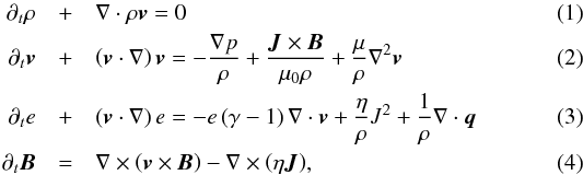 where ρ represents the density, v the flow velocity, e = (γ − 1)P/ρ the specific internal energy of the gas, and B the magnetic field. The magnetic resistivity and dynamical viscosity are represented as η and μ. The current density is J = ∇ × B/μ0, and μ0 is the magnetic permeability.
The heat flux q includes the contributions from the viscous heat flux qvisc and from the conductive heat flux qc. The former accounts for the dissipation of shear flows, according to  (5)where
  is the isotropic (shear) viscous stress tensor with components
 ![\hbox{${\cal D}_{ij}=-2\mu\left[e_{ij}-\frac{1}{3}\left(\nabla\cdot\vec{v}\right)\delta_{ij}\right]$}](/articles/aa/full_html/2015/04/aa23358-13/aa23358-13-eq22.png) , where eij is the strain rate tensor. The latter corresponds to a flux-limited Spitzer-Härm (SH) magnetic-field-aligned conductivity. The SH conductive flux vector is defined as
, where eij is the strain rate tensor. The latter corresponds to a flux-limited Spitzer-Härm (SH) magnetic-field-aligned conductivity. The SH conductive flux vector is defined as  (6)where
  is the unit vector in the direction of the magnetic field and κ0 the SH conductivity coefficient (Spitzer & Härm 1953). A correction is applied to this term, so that the conductive heat flux becomes independent of ∇T for extremely large temperature gradients (see, e.g., Orlando et al. 2010; West et al. 2008). This correction relies on the definition of the saturation flux qsat
 (7)where φ is an arbitrary coefficient set to 3 / 2 in our simulations,
  is the sound speed, where γ = 5 / 3 is the ratio of specific heats and T ∝ p/ρ is the fluid temperature. The value of φ was determined following the analysis by Cowie & McKee (1977), and by trying a few different values for this parameter (~0.1−1.5) and verifying that its variation has a negligible effect on our specific flux-rope setup (we decided to use the upper and more conservative value of the tested parameter range).
The total conductive heat flux is then defined as  (8)We also considered in some cases an additional right-hand side term for the energy equation (Eq. (3)) to account for the radiative losses in the corona. This term is written as
  , where n is the numerical density and
  represents the cooling rate as a function of the temperature for an optically thin plasma. The value of is obtained from tabulated data calibrated for solar abundances (generated with CLOUDY 90.01, Ferland et al. 2013). We did not use this radiative cooling term systematically because its amplitude is small for the model parameters we chose (see Sect. 2.3), and including it significantly increases the numerical cost of the simulations. We nevertheless verified the effects of radiative cooling by running some simulations with this term turned on (see Sect. 3.2).
The MHD Eqs. (1) to (4) are solved in dimensionless form using the dimensional scaling factors dependent on the assumed characteristic magnetic field strength B0, the characteristic length-scale L0, and the characteristic density ρ0. Hence, the characteristic speed is the Alfvén speed  , the characteristic time-scale is t0 = L0/v0, the characteristic temperature is given from the equation of state
 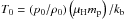 (where μH is the mean molecular mass for a fully ionised hydrogen gas, mp is the proton mass, and kb is the Boltzmann constant) and the characteristic resistivity is η0 = L0V0.
We integrated this set of equations using the numerical code PLUTO (Mignone et al. 2007). Our setup consists of a fixed and uniform Cartesian grid with coordinates x, y, and z such that the magnetic flux-rope is oriented in the z-direction. The foot-points of the magnetic flux-ropes lie on the planes z = 0 and z = L0. The system is advanced in time using explicit time-stepping (Hancock scheme associated with a low-diffusion slope limiter) and a hlld solver (Miyoshi & Kusano 2005), except for the diffusive terms (the viscous, resistive, and conductive terms). Spitzer-Härm (SH) thermal conduction, in particular, makes the explicit integration step become prohibitively small. For this reason we integrated all the parabolic (i.e., diffusive) terms using a super time-stepping implicit scheme (STS), while the other terms follow the usual explicit scheme. The solenoidal condition (∇·B = 0) is ensured by a hyperbolic divergence cleaning technique (Dedner et al. 2002). The boundary conditions are periodic in the x and y directions and are line-tied in the z direction (i.e., the loop foot-points are line-tied; see Sect. 2.3). The line-tying condition was applied at the external boundaries (faces) of the outermost numerical cells. The velocity, density, pressure, and magnetic field were held fixed there. The diffusive coefficients are null at these boundaries to ensure that the magnetic field remained line-tied. The velocity gradients were minimised in the first two numerical cells adjacent to the boundaries to ensure numerical stability (in a way similar to that in Aulanier et al. 2005). A finite conductive heat flux was allowed across the top and bottom boundaries (acting as a proxy to the heat flux from the corona to the chromosphere across the transition region; see Sect. 3.1 for a discussion of these effects).
2.2. Estimating the thermal X-ray emission
We estimated the thermal X-ray emission as a post-processing step based on the spatial distributions of density and temperature obtained from the MHD simulations. We focused on the continuum emission in the 1−25 keV photon energy range (at the low end of the detection range for RHESSI and for the future Solar Orbiter/STIX spectro-imager), and on how its properties evolve in time following reconnection events in the simulated flaring loops (see the discussion in Sect. 4.2). The continuum thermal X-ray emissivity of a fully ionised hydrogen plasma with uniform number density n and temperature T at a given photon energy hν is 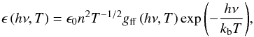 (9)where gff(hν,T) is the Gaunt factor for free-free bremsstrahlung emission, and the coefficient ϵ0 is 6.8 × 10-38 if the emissivity is to be expressed in erg cm-3 s-1 Hz-1 (Tucker 1975). We used the following piece-wise approximation to the Gaunt factor
 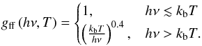 (10)The corresponding photon flux density emitted at the photon energy hν is defined as
 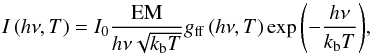 (11)where EM is the emission measure n2V of a finite volume of plasma (of density n and temperature T), and the coefficient I0 is 1.07 × 10-42 for a photon flux measured at a distance of 1 AU and 1.20 × 10-41 for a photon flux measured at the Solar Orbiter perihelion (~0.3 UA), if the photon flux density is expressed in units of photons cm-2 s-1 keV-1. The total photon flux over a given spectral band is computed by integrating Eq. (11) over the corresponding range of values of hν. We computed the photon flux at different photon energies for each individual grid cell (i.e., volume element), each one having a one-value emission measure (note that the density varies in the loop) and temperature. As the corona is optically thin to X-ray radiation, the total flux emitted is obtained by adding the individual contributions over the whole loop (or over a region of interest).
We estimated the distributions of  in our simulations by computing the total emission measure of the plasma regions whose temperature lies within successive temperature intervals at a given time. That is, the emission measure is defined as a function of temperature as
  (12)where the index k runs through all the plasma elements (grid-cells in the simulations) that lie within the temperature interval [T,T + δT], nk and δVk are the number density and volume of each element. In other words, we first computed a temperature histogram with a given temperature bin size δT. Then, we verified which grid cells have a temperature T within each of the bins and summed over all the corresponding individual EM. Variations in density in the plasma at a given temperature are therefore accounted for.
2.3. Model, dimensions, and parameters
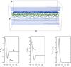 |
Fig. 1 Initial conditions for the standard case (magnetic field properties alone; see Table 1). The three-dimensional picture on the top shows a sample of magnetic field lines (coloured according to the magnetic field strength). The plots below show the amplitude of the magnetic field components Bz and Bθ, the current density components Jz and Jθ (with J = ∇ × B/μ0) and the twist angle |

We considered here twisted magnetic flux-ropes embedded in a region of background magnetic field that is uniform and aligned with the flux-rope axis direction (the z-direction in our setup). The flux-ropes are straight, and the effects of the large-scale loop curvature are therefore neglected. The initial state of the system is force-free and in hydrostatic equilibrium. The background medium is characterised by a uniform magnetic field oriented in the  direction, a uniform density ρ, and a uniform gas pressure
  , where β represents the ratio of gas to magnetic pressures. We set the parameter β to the value 0.01 to correctly represent the dynamics of the magnetically dominated corona. The twisted magnetic flux-rope is, initially, perfectly cylindrical with its main axis oriented in the
  direction. Its characteristic magnetic field is B = B0êz (at its axis). Its length L0 matches the numerical domains length, and its radius is denoted r0. The plasma is initially stationary everywhere in the domain (v = 0). For simplicity, we defined the flux-rope magnetic field components in the cylindrical components Br, Bθ , and Bz such that r is the distance to the z-aligned flux-rope axis and θ = tan-1(y/x) is the azimuthal angle. The radial component Br is null everywhere. The components Bz, and Bθ are defined in terms of the twist parameter λ. Inside the flux-rope (i.e., for r ≤ r0)
 ![\begin{eqnarray} \label{eq:flux_rope_field_in} B_{\theta} &=& B_0 \lambda \frac{r}{r_0} \left( 1 - \frac{r^2}{r_0^2} \right)^3 \\ B_z &=& B_0 \left[ 1 - \frac{\lambda^2}{7} + \frac{\lambda^2}{7}\left( 1 - \frac{r^2}{r_0^2}\right)^7 - \lambda^2\frac{r^2}{r_0^2} \left( 1 - \frac{r^2}{r_0^2}\right)^6 \right]^{1/2} , \nonumber \end{eqnarray}](/articles/aa/full_html/2015/04/aa23358-13/aa23358-13-eq104.png) (13)and outside (i.e., for r>r0)
(13)and outside (i.e., for r>r0)  (14)as in Hood et al. (2009), Botha et al. (2011), Gordovskyy & Browning (2012), and Gordovskyy et al. (2013). The flux-rope magnetic field matches the background field at r = r0. The value of the parameter λ controls the twist in the flux-rope, rendering it more or less susceptible to the kink instability. The magnetic field becomes purely axial everywhere in the domain for λ = 0 (because Bθ = 0 and Bz = B0 in that case). The highest value of the twist parameter is λ ≲ 2.438, ensuring that the square-rooted polynomial in Eq. (13) is positive. The flux-rope field is purely toroidal (Bz = 0) for this limiting value of λ. The threshold for the kink instability depends both on the specific transverse twist profile considered and on geometrical parameters such as the flux-rope aspect ratio (Bareford et al. 2013). In our case, and for an aspect ratio L0/r0 = 10, the kink instability is prone to develop for λ ≳ 1.6. Empirically, and given the constraints imposed by diffusive time in our simulations, we verified that cases with λ ≤ 1.8 are impractical to use. We deliberately chose higher values for the twist parameter (λ = 2.0−2.4) to guarantee that the kink instability would develop with the least amount of spurious magnetic diffusion. The system will remain stationary (in its initial state) for an indefinite amount of time unless some form of asymmetry is introduced. Hence, we introduced a small amplitude seed perturbation in the form of a harmonic velocity noise that is highest at the centre of the domain and null at the boundaries. The actual form of the perturbation is unimportant to the outcome of the simulations as long as its amplitude remains much smaller than the system’s characteristic sound and Alfvén speeds. This mechanical perturbation can be thought of as representing any kind of disturbance in the dynamical corona.
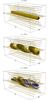 |
Fig. 2 Three snapshots showing the temporal evolution of the magnetic field and the current density in the standard case (Table 1). Blue lines: magnetic field-lines initially placed near the axis of the flux-rope. Yellow lines: magnetic field-lines initially crossing the periphery of the flux rope and the background field. The yellow volumes represent the current density distribution (light/dark yellow corresponding to moderate/strong amplitudes). The inner (blue) magnetic field-lines are concentrated well within the current-carrying region (hence hidden in the first two panels) before the reconnection event takes place. The instants represented correspond to the initial state (t = 0 s), to the peak in magnetic energy release rate (t = 75 s), and to the relaxation phase (t = 118 s). |
Figure 1 shows a three-dimensional rendering of the magnetic field at the initial state of one of our simulations. The blue and green lines represent magnetic field-lines connected, respectively, to the twisted flux-rope and the background field. The figure to the right shows the distribution of the twist angle  in a plane perpendicular to the flux-rope axis. Note that the twist profile
  is controlled by the parameter λ and that the effects of varying the latter can translate into qualitatively different twist distributions.
The rectangular numerical grid has a length Δlz = L0 = 10 and a width Δlx = Δly = 5 in normalised units, and the grid dimension is 2563, with the grid-cells thinner in the transverse x and y directions than in the longitudinal z direction. Other resolutions were tested, such as 256 × 256 × 512 and 512 × 512 × 1024 (i.e., different grid-cell sizes and aspect ratios) to verify numerical stability. The flux-rope radius is r0 = 1 in the standard case. The characteristic magnetic field strength B0 equals 2, the characteristic density equals unity, and the characteristic temperature is T0 = 5 × 10⁻³. The flux-rope Alfvén and sound longitudinal crossing time-scales therefore are τA = 5 and τs ≈ 110. To scale the simulations to coronal values, we set  ,
,  and
and  . As a consequence, the coronal temperature is
  (a typical coronal loop temperature) and the Alfvén and sound crossing times are
  and
and  . The typical size of the grid-cells then is ~100 km in the transverse directions (x and y) and ~200 km in the longitudinal direction (z). The flux-rope viscous and resistive time-scales τη = a2/η and τμ = ρa2/μ are ~500τA. The magnetic resistivity is uniform, with a value 2 × 1014 cm2 s-1, which more than ensures the stability of the numerical scheme, with magnetic Reynold’s numbers never larger than ~1 at the grid-scale (for comparison, this value is close to those reported by, e.g., Bingert & Peter 2011). As a consequence, the bulk magnetic diffusion at large scales is non-negligible, and low-twist scenarios become harder to calculate than high twist cases. This set of parameters ensures that the twisted flux-ropes are kink unstable, and that they are strongly and quickly heated during the first phase of the evolution of the instability (see Sect. 3), after which they experience a cooling phase. We expect plasma cooling to be dominated by thermal conduction rather than by radiation for our typical loop parameters during the dynamical time-scales we considered (~102−103 s; the estimated conductive to radiative cooling time-scales being of about 10-5−10-4 during that period). Hence, we did not account for the latter in most cases. We verified a posteriori that this assumption was correct (see Sect. 3.2 and Fig. 9). It should be noted, nevertheless, that the cooling time-scales depend strongly on the choice of model parameters. For example, substantially denser and colder loops could reach higher values for the ratio τcond/τrad, or even switch from conductively cooled to radiatively cooled regimes during the course of the relaxation phase (see, e.g., Cargill 1994; Cargill et al. 1995; Klimchuk et al. 2008). We did not consider such cases here. Table 1 shows a summary of our standard choice of dimensional scaling parameters, which we hereafter refer to as standard case. Variations to the standard case are referred to with the names in Table 2.
Summary of the model parameters and of the standard choice of physical dimensions (standard case).
Summary of the comparative cases and of the parameters that were changed with respect to those in the standard case.
3. Results
We describe below the different stages of the temporal evolution of the simulated kink-unstable loops. The main geometric features and the global dynamical behaviour of the system agree well with previous studies, as expected (e.g., Hood et al. 2009; Botha et al. 2011; Gordovskyy & Browning 2012). Our main contribution to this body of research lies in studying the properties of thermal X-ray emission of these systems. Section 3.1 describes the temporal evolution of the magnetic field and currents during the flaring episode and the overall energy balance. Section 3.2 describes the X-ray emission properties in detail. Section 3.3 describes the development of a multi-temperature plasma in the flaring loops. These results are discussed with respect to X-ray observations of flaring loops in Sect. 4.
3.1. Dynamical evolution
The temporal evolution of the kink-unstable twisted flux-rope is divided into three distinct phases, which we name the linear phase, the saturation phase, and the relaxation phase. Figure 2 shows a few snapshots that illustrate these phases. The yellow and blue lines represent magnetic field-lines rooted at the top and bottom boundaries, the yellow volumes represent the current density distribution. The twisted flux-rope is initially at rest, and the kink instability is triggered after an initial perturbation breaks its perfect cylindrical symmetry (perturbing its magnetic tension balance). From then on (and as long as the linear phase of the instability lasts), the flux-rope kinks about its axis and expands outwards. The plasma is heated by compression ahead of the boundaries between the expanding regions and the background medium. Helical-shaped and thin current sheets form and grow at these interfaces. At a certain point, the flux-rope magnetic field begins to reconnect with the background field, and the linear instability (exponential growth) saturates. The system’s magnetic geometry is quickly reconfigured, the peripheral current sheets begin to fragment and decay in amplitude, and strong and localised heating occurs there. The saturation time-scale directly depends on the values assumed for the diffusive coefficients and weakly depends on the amplitude of the initial perturbation. In particular, lower magnetic resistivities allow the plasma compression to proceed for a longer period of time and lead to stronger peak currents. In our numerical setup, the saturation time-scale is of the order of 4−5 Alfvén crossing times. From then on, the global magnetic field slowly converges to a state with lower twist, closer to a potential field configuration. During the saturation and relaxation phases, the current density looses its initially smooth and cylindrically symmetric distribution (see the plots in Fig. 1 and the first image in Fig. 2) and assumes a more intermittent spatial distribution, until it eventually fades away.
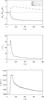 |
Fig. 3 Temporal evolution of the variations in total kinetic, magnetic, and internal energies (ΔEcin, ΔEmag, ΔEint), average current density squared ⟨ j2 ⟩, and average linear momentum ⟨ ρv ⟩ in the standard case (in dimensionless units). The grey lines in the top panel represent the same quantities for a case without thermal conduction for comparison. The total kinetic energy is always lower than the magnetic and internal energies. The thermal conductive flux then begins to grow fast as the plasma quickly heats up locally (as a result of the ohmic dissipation) and is responsible for the decay in internal energy during the relaxation phase (note that in our setup the conductive flux can transport heat outwards through the loop footpoints). |
Figure 3 shows the absolute variations of total kinetic, magnetic and internal energies in the system as a function of time, as well as the temporal evolution of the average current density and momentum. The total kinetic, magnetic, and internal energies are defined as  ,
,  and Eint = ∫VρedV. The overplotted grey lines show the same quantities, but for a model without thermal conductivity (Eqs. (6) to (8)). The initial excess of magnetic free energy is predominantly transferred into thermal energy, while only a small fraction is converted into kinetic energy. The plasma flow velocities remained low at all times (below 0.1cs), despite the initial impulsive acceleration and the low plasma β. The variations of total internal energy ΔEint and total magnetic energy ΔEmag are almost perfectly reciprocal during the linear phase (and especially so in the non-conductive case). During the saturation phase, the strong and localised increases in plasma temperature make the thermal conduction very efficient. As a result, the maximum ΔEint attained is slightly lower than in the non-conductive case. From then on, the total internal energy slowly decays and approaches its initial value. This occurs because thermal conduction is allowed to let heat flow through the loop foot-points in our setup. If this were not the case, the magnetic loops would reach higher maximum temperatures and would almost not cool down after the saturation phase, keeping ΔEint at a stable level. The current density peaks at about t = 110 s, which roughly corresponds to the instant represented in the second panel in Fig. 2, just before the magnetic reconnection event starts. The current density quickly decays from that moment on (as the magnetic field is reconfigured and relaxes). The plasma, initially at rest, is accelerated (essentially outwards) during the linear phase of the instability. After the initial push, the dominant large-scale flows consist of circulation patterns around the flux-rope, with the amplitude of the flows remaining very subsonic at all times (i.e., with no accumulation of mass at the boundaries of the domain). After reconnection is triggered, some longitudinal acceleration appears for a short period of time in some places of the flux-rope. This is at the origin of the second peak in the momentum curve (third panel in Fig. 3). These large-scale bulk flows are attenuated during the subsequent relaxation phase, but the smaller scale flows persist. Longitudinally propagating low-amplitude oscillations triggered during the initial burst survive for a long period of the relaxation phase (at least up to t = 1000 s).
3.2. Thermal X-ray emission
We focus now on the properties of the thermal bremsstrahlung X-ray emission deduced from our simulations.
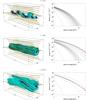 |
Fig. 4 Temporal evolution of the magnetic field, of the emissivity at 10 keV (as defined in Eq. (9)), and of the total emission spectrum (Eq. (11)) in the standard case (see movie online). The instants represented correspond, from top to bottom, to the linear phase (t = 75 s), the saturation phase (t = 90 s) and the relaxation phase (t = 475 s). Left column: three-dimensional renderings of the magnetic field (blue and yellow lines, as in Fig. 2) and of emissivity (green volumes) at these instants. Right column: corresponding emission spectra between 1 and 20 keV. The red lines show the spectra at the same instants as the figures to the left, and the light to dark grey lines show spectra at some preceding instants (with 2.5 s of time-delay between each line), hence giving an idea of the quickness of the evolution of the spectra. The black dashed lines show the initial (t = 0 s), end of linear phase (t ≈ 75 s) and peak spectra (t ≈ 90 s). (An associated movie is available online.) |
Figure 4 shows a sequence of three snapshots of the magnetic field and of three-dimensional renderings of the emissivity at 10 keV (see Eq. (9)), accompanied by the photon spectra at 1 AU (see Eq. (11)) at the same instants by the total loop volume. The instants represented are t = 75 s (end of the linear phase), t = 90 s (during the saturation phase and peak of emission), and t = 475 s (during the relaxation phase). The blue and yellow lines represent magnetic field lines initially within the twisted flux-rope and the background field (as in Fig. 2). The green volumes represent the regions of the plasma emitting strongly at 10 keV. The red lines in the plots to the right of the figure show the total photon spectra at 1 AU at the same instants as the figures to the left, and the light to dark grey lines show spectra at some preceding instants (hence giving an idea of the quickness of the evolution of the spectra). The time interval between consecutive grey lines is 2.5 s. The black dashed lines show the spectra at the initial state (t = 0 s), at the end of the linear phase (t ≈ 75 s), and the peak spectra (t ≈ 90 s).
The first signs of thermal emission appear close to the axis of the flux-rope in small discontinuous patches heated by compression. These very quickly extend along the corresponding magnetic field-lines, hence forming the filamentary and helical emission pattern which highlights the writhe (large-scale twist) of the flux-rope. A strong helical current sheet then begins to form around the flux-rope (in the zones more strongly compressed against the external medium; see Fig. 2, second panel). The ohmic heating grows quickly there, and the emission concentrated in these outermost layers overcomes that of the first sources of emission (as shown clearly in the first two panels of Fig. 5). This enhanced emission assumes the shape of a helical surface wrapped around the axis of the flux-rope, which coincides with the zones of maximal current density at that instant (cf. the second panel in Fig. 2 with the second panel in Fig. 5, both at 75 s). The emission rapidly grows as the kink instability proceeds, filling the adjacent zones and forming a compact and continuous emitting structure (see the second row in Fig. 4, left side, at t = 90 s). During the initial phases (for t ≤ 65 s), the photon flux spectrum is increased at a steady pace (first row in Fig. 4, plot on the right side), mostly as a result of the moderate compressional heating taking place at the emitting regions.
When the saturation phase is reached, the magnetic field is quickly reconfigured by reconnecting with the external field (see the second row in Fig. 4, t = 90 s). A strong ohmic heating burst accompanies the reconnection process. The total photon flux increases very sharply (note the larger gaps between consecutive lines in the plot to the right), and the photon spectrum increases dramatically at high energies. This spectral hardening occurs as the loop plasma transitions from a state with nearly uniform temperature to a state with a broad temperature distribution (with an extended upper tail, reaching as high as ~35 MK; cf. Sect. 3.3 and Fig. 10).
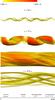 |
Fig. 5 Detail of the continuum emission at 5 keV at different instants for the standard case. The orange/red colour-table represents the emissivity, as defined in Eq. (9). Dark red represents ϵ = 1013 erg s-1 cm-3 Hz-1, a factor 10 stronger than yellow. The instants represented correspond, in order, to the final moments of the linear phase (t = 65 s), to the saturation phase/peak of emission (t = 75 s), to the early relaxation phase (t = 245 s), and to the later relaxation phase (t = 475 s). The scale at the bottom shows the corresponding pixel size for RHESSI and STIX both at the aphelion (~1 AU) and perihelion (~0.3 AU) of the spacecraft orbit. (An associated movie is available online.) |
During the relaxation phase, the emission begins to decay slowly while becoming again more fragmented and concentrated in field-aligned filaments (last row in Fig. 4). The plasma cools down globally (see Fig. 3), but maintains its multi-thermal character for a very long time (see Sect. 3.3). The photon spectrum hence decays as a whole approaching the initial one, but without becoming as soft as initially for the whole duration of the simulations.
The fine structure of the emission is shown in more detail in Fig. 5. The four panels represent volume renderings of the emissivity at 5 keV. The colour table covers a factor 103 in emissivity, from light yellow to dark red (see the inset colour-scale at the top of the figure). The scale at the bottom indicates the length of the loop (50 Mm) as well as the corresponding pixel sizes for RHESSI and STIX (at aphelion and perihelion of the orbit planned for the Solar Orbiter spacecraft). The instants represented illustrate the final moments of the linear phase (t = 65 s), the saturation phase (t = 75 s, when the current density is highest), the beginning of the relaxation phase (t = 245 s), and a later moment of the relaxation phase (t = 475 s). The first traces of thermal emission appear oriented along a few (and only a few) magnetic field-lines. This occurs because the thermal conductivity efficiently transports heat along the magnetic field (and not across), and because the plasma heating sources are initially very discontinuous in space. Note that the initial mechanical perturbation breaks the initial cylindrical symmetry, and that the resulting small-scale plasma flows are inhomogeneous from early on. Hence, reconnection is not forced in a perfectly symmetrical way. Emission nonetheless displays a rather symmetrical large-scale pattern.
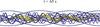 |
Fig. 6 First instant in Fig. 5 plotted together with some magnetic field-lines (also for the standard case, and with the same colour-table). The thermal X-ray emission pattern highlights only parts of the flux-rope with low twist during the initial phases of the flare. Later on, the emission pattern fills the entire flux-rope volume, but the flux-rope will have lost much of its twist by then. Throughout the flare evolution, the most highly twisted magnetic field-lines are very rarely visible. |
For a short period of time, the bulk of the thermal emission effectively traces a few magnetic field-lines in the flux-rope. The emission pattern then displays a clear helical pattern, with a perceived twist of about three turns (or a twist angle of 6π) at this instant. Note that this value is much lower than the initial magnetic twist angle in this region (8−18π; see Fig. 1). This difference occurs for two reasons. The first is that the loop has already lost an important fraction of its twist when the plasma becomes hot enough to produce distinguishable emission patterns. The second reason is that the corresponding field lines are well within the twisted flux-rope and hence have lower pitch angles (and lower total twist) than the more external ones (see the twist radial profiles in Fig. 1). This effect is seen more clearly in Fig. 6, where a sample of magnetic field-lines is plotted together with the emission pattern at the same instant. The bulk of the emission is indeed concentrated closely to the kinking flux-rope axis and is surrounded by more strongly twisted field-lines (for which there are no traces of emission at this moment). This emission pattern is only visible briefly, however (10−15 s). The second panel in Fig. 5 shows the moment when ohmic dissipation in the helical current sheet formed around the kinking flux-rope becomes important (compare with the second panel in Fig. 2). Note that the emission peak does not occur at the same time as the peak in ohmic heating rate (proportional to |j2|; see Fig. 3), but slightly later (about 20 s later). The third panel shows the beginning of the relaxation phase, when the emission becomes almost cylindrically symmetric. The last panel represents the later relaxation phases. The emission again traces a more threaded pattern, qualitatively similar to those in coronal loops observed in the EUV range. The apparent radius of the loop (the radius of the emitting plasma) varies as a function of time in our simulations (cf. Jeffrey & Kontar 2013). The width of the emitting region is initially smaller than that of the actual magnetic flux-rope, but increases quickly as the instability proceeds. It then stabilises during the relaxation phase as the emission fades away. The typical widths of the filamentary emission patterns described above are below the maximum spatial resolution obtained by RHESSI or by the future STIX instrument (Solar Orbiter). The overall helical structure would probably be unnoticed by these instruments. Later on and for most of the flaring episode, the emission pattern should be visible only as a cylindrically symmetric structure (with no apparent traces of helicity).
Figure 7 shows a series of light curves computed for different photon energy bands. The light curves were computed by integrating the spectra in Fig. 4 over each energy band at all instants. Emission from the whole numerical domain was taken into account. The light curves are normalised to their highest value to facilitate the comparison (the peak values differ by more than two orders of magnitude between the lowest and highest energy bands). The thermal X-ray emission peaks during the impulsive phase and decays asymptotically during the relaxation phase. The light curves peak almost synchronously. The longest time lag between different peaks is just slightly higher than 15 s, with the highest energy band (12−25 keV) preceding all the others, and with the lowest energy band (1−3 keV) being last. However, the lower energy light-curves begin to grow earlier and more progressively than the higher energy ones. More importantly, the decay time-scale is longer for the lower energy bands and shorter for the higher energy bands. This is consistent with the fact that thermal conduction efficiently dampens the high-temperature peaks because the conductive flux is proportional to T5 / 2∇T (see Eq. (6)).
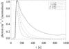 |
Fig. 7 Light curves of X-ray thermal emission at different energy bands for the standard case. The curves are all normalised to their peak value. The inset key shows which energy band corresponds to each line in the plot. Higher energy bands decay faster, lower energy bands decay more slowly. The longest time lag between different peaks is of about 10 s (the lowest energy bands peak earlier). |
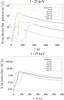 |
Fig. 8 Top panel: light curves for different cases in the 1−25 keV range. The cases represented are the standard case, a non-conductive case, a low-twist case, a case with a flux-rope twice as thin, a case with a flux-rope twice as long, a strong B-field case (twice as strong), and a case with strong B-field and a denser flux-rope such that the plasma beta and characteristic Alfvén speed are maintained (see the inset legend). Bottom panel: the same light-curves but with rescaled time and photon flux. The highest emission is approximately proportional to |
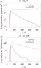 |
Fig. 9 Light curves for the standard case, for the standard case with radiative cooling, and for the standard case without thermal conduction. As expected, radiative cooling has very little effect for the chosen loop parameters. Conductive cooling (and leakage), on the other hand, plays a very important role during the whole relaxation phase. Top panel: light curves in the 3−6 keV range. Bottom panel: light curves in the 12−25 keV range. |
Figure 8 (top panel) shows a series of light curves for different cases, all in the broad 1−25 keV photon energy range. The cases represented are the standard case (black line), a low-twist case (blue line), a case with a flux-rope twice as thin (continuous green line), a case with a flux-rope twice as long (dashed green line), a weak B-field case (twice as weak; continuous orange line), and a case with strong B-field (by a factor 2) and a denser flux-rope (denser by a factor 4) such that the plasma beta and characteristic Alfvén speed are maintained (dashed orange line).
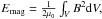
Variations in flux-rope geometry and magnetic field amplitude lead to different emitted peak fluxes and to different peaking time-scales. The strongest photon flux amplitude scales approximately linearly with the flux-rope’s initial magnetic energy and initial density. This can be easily seen by comparing the standard case (with initial magnetic energy  ) with the cases with a flux-rope twice as long, with a flux-rope twice as thin, and with a magnetic field amplitude twice as strong (but the same initial density n0). They have initial magnetic energies that are
  ,
,  and
and  , respectively. The corresponding peak fluxes deviate from that of the standard case by factors of 2.0, 1 / 3.67, and 4.2. The case with a strong-field (twice as strong) and denser flux-rope (four times as dense) shows that the peak emission also depends on the density, such that the emitted flux is proportional to
  . This is physically sound because the primary source of plasma heating is the initial (free) magnetic energy and because the resulting temperature increase is proportional to the transferred energy per particle (T0 ∝ 1 /n0). The photon flux is proportional to
  , and so the final scaling factor is also proportional to n0. The time-scales required to achieve the peak flux τpeak are proportional to r0/v0 (ratio of flux-rope radius to characteristic Alfvén speed), at least for all cases with the same transverse twist distribution. Indeed, the case with a thin flux-rope (twice as thin) has a peaking time that is about half that of the standard case, and so does the case with a strong magnetic field (twice as strong, and so with a characteristic Alfvén speed v0 twice as high) but with same radius r0. Taking the latter case and increasing the initial density ρ0 such that the initial characteristic Alfvén speed is maintained with respect to the standard case again leads to the same peaking time. Note that the expression
 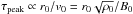 remains constant if the loop length L0 varies while keeping
  constant (compare the black and dashed green curves in Fig. 8). The bottom panel in Fig. 8 shows the same light curves normalised by the scaling factors discussed above. The curves fall much closer together, showing that these scaling factors proposed work well for an extended evolution period of the simulated coronal structures.
For completeness, we discuss two additional cases that are similar to the standard case (same loop parameters), but one with radiative cooling turned on and the other with thermal conduction turned off (see Sect. 2.1). Figure 9 compares the light curves obtained for the standard case (represented with continuous lines), for the case with radiative cooling (dotted lines), and for the case without thermal conduction (red continuous line). The total effect of the radiative cooling remains very weak during the whole simulated time, thus confirming that plasma cooling by radiation is negligible for the loop parameters we chose.
Thermal conduction (and foot-point heat leakage) has, on the other hand, a strong effect. The initial growth phase in the latter is similar in the conductive and non-conductive cases, but the emission peak is stronger in the latter (as the plasma reaches higher maximum temperatures without thermal conduction). More importantly, the relaxation phase is very different in the non-conductive case, as the plasma does not cool down globally and conserves its internal energy (see Fig. 3). Hence, the emitted photon flux does not decay in that case, as would be expected from observed flares. Thermal conduction is therefore a requirement for the correct modelling of the thermal emission in solar flares.
3.3. Temperature distribution and emission measures
The thermal X-ray spectra displayed in Fig. 4 show that the plasma becomes intrinsically multi-thermal after the kink instability is triggered. A small (but strongly emitting) fraction of the flux-rope plasma is heated up to temperatures one order of magnitude above that of the background plasma. More high-energy photons are produced, and the emission spectrum is elongated into the high photon-energy end.
We tried to fit the photon flux density in Eq. (11) to the spectra we obtained from the simulations to determine the best-fit values for the flare temperature and emission measure (Te and EMe hereafter). Note that this expression assumes a uniform temperature Te for the emitting plasma (which can be seen as an effective temperature). These fits were performed for different instants of the simulations to give an indication of the temporal evolution of the fitted parameters and to allow comparisons with the original simulation data. We found that the thermal spectra can be well approximated by the emission of a volume of plasma at uniform temperature during most of the linear phase (for t< 80 s, roughly). The fitted spectra remain very close to the original spectra, and Te ≈ ⟨ T ⟩ (where ⟨ T ⟩ is the volume-averaged temperature in the simulation). This changes dramatically as the saturation phase approaches and magnetic reconnection starts taking place. The ohmic heating generates a temperature distribution in which a very long upper tail and emission at higher energies suddenly becomes more important, which hardens the spectra. The fitted curves hardly match the original spectra during the saturation phase in the whole energy range we considered here (1−25 keV). A multi-temperature fit would probably yield more consistent results (we did not attempt such techniques in this manuscript).
The top panel in Fig. 10 represents the temporal evolution of the plasma temperature in our simulations. The maximum temperature Tmax is represented by a dotted-dashed line, the volume-averaged temperature ⟨ T ⟩ by a dotted line. The continuous line represents the volume-averaged temperature of the bulk of the hot plasma component, which we call Thot hereafter (providing an indication of the effective flare temperature). The loop plasma undergoes a strong and quick initial heating event and cools down more slowly afterwards. The actual cooling time-scale is naturally longer than the estimated conductive cooling time-scale. Small sporadic heating events with finite duration continue to occur during the relaxation phase as the magnetic field tries to approach a potential state and contribute to maintaining the loop plasma at a hotter temperature than the background in spite of the strong conductive cooling. The bottom panel displays a histogram of the temperature at one selected instant of the simulation (t = 125 s, just after the saturation phase) with markers identifying the values of Thot and ⟨ T ⟩ at that instant. The plasma temperature distribution develops an extended upper tail during the saturation and beginning of the relaxation phase. It indicates a cold plasma component and a hot flare component. The lower temperature peak (background plasma) is a consequence of the choice of initial conditions, however, and broadens as the simulation proceeds. The higher temperature peak is clearly visible during the first few minutes after the saturation, but is less pronounced and spreads outs afterwards under the action of the thermal conduction. Overall, the temperature distribution is broad and continuous, extending across more than one order of magnitude.
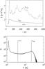 |
Fig. 10 Top panel: temperature Thot corresponding to the average temperature of the bulk of the hot plasma component that develops after the saturation phase (continuous line). The maximum temperature Tmax and the average temperatures ⟨ T ⟩ at each instant are represented by a dotted-dashed line and a dotted line. Bottom panel: histogram of the plasma temperature in the simulation at t = 125 s. The vertical lines in the bottom plot mark the positions of the hot-plasma-component temperature and of the volume-averaged temperatures (Thot and ⟨ T ⟩). |
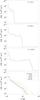 |
Fig. 11 Emission measure as a function of temperature |
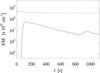 |
Fig. 12 Total emission measure (EM) of the cold and hot plasma components as a function of time (represented with a dashed and a continuous line). We define as “hot” all plasma at a temperature above 9 MK (cf. Sylwester et al. 2014). |
A more interesting spectral diagnostic tool consists of considering a temperature-dependant emission measure in the function I(hν,T) (see Eq. (11)). We computed a time-series of curves directly from our simulations (see Sect. 2 for a description of the method used). Figure 11 shows a sample of these curves for three representative instants of our standard case. These are t = 12 s (linear phase), t = 63 s (start of the saturation phase), and t = 125 s (early stage of the relaxation phase). Then, a series of curves corresponding to the relaxation phase for different cases are plotted together (at about t = 25τA for each of the cases represented). These correspond to a case with lower twist, to a flux-rope twice as thin, to a flux-rope twice as long, to a strong B, and to denser flux-rope (see the inset caption). The dotted black line in the bottom panel of the figure is a guideline indicating the slope of the curve EM ∝ T-4. The initial distribution is narrow (as expected for an isothermal plasma) and centred at T = T0 = 1.2 × 10⁶ K. It then quickly extends into the higher temperature range, especially as the plasma is strongly heated up by ohmic diffusion during the saturation phase. A transient bump forms in the higher temperature part of the  distribution, in a manner which is qualitatively similar to that of the temperature distribution described above (see Fig. 10). The dominant plasma populations are then composed of the unheated background plasma (i.e., at the initial temperature T0) and the strongly heated plasma. Significant emission measure is then found for a plasma with a temperature around 20 MK. The EM profile afterwards slowly converges to a power-law distribution as the hot component spreads out and disappears. As the dotted guidelines indicate, the curve settles close to EM ∝ T-4 for T ≳ 2 × 10⁶ K. Fitting the curve to a power-law between T = 2 × 10⁶ K and T = 1 × 10⁷ K yields a power-law exponent −4.2 ± 0.1. We found the same behaviour in all the simulation runs we performed, with the evolving in the same way and converging to a power-law with the same index (but different absolute values). The last panel in Fig. 11 shows a few illustrative cases, for which we varied the flux-rope length, thickness, level of twist and magnetic field strength. Cases with different numerical resolutions, viscosity, and magnetic resistivity were also verified. The only exception we found was the case similar to the standard one but without thermal conduction. In the latter, a fraction of the heated plasma reaches maximum temperatures higher by a factor ~5 (cf. Botha et al. 2011), and remains hot in the lack of a cooling mechanism as efficient as the Spitzer-Härm thermal conduction. This naturally translates into a EM distribution extending up to higher temperatures and to a flatter power-law.
Figure 12 shows the temporal evolution of the total emission measure of the hot and cold plasma components separately. We here define hot (cold) plasma as all plasma with a temperature above (below) a threshold of 9 MK, as in Sylwester et al. (2014). The emission measure of the hot plasma component increases abruptly during the linear/impulsive phase of the kink instability, reaching a highest value of 5 × 1047 cm-3 in ~125 s. It then slowly decays during the relaxation phase. This translates into an inverse variation of the total emission measure of the cold component with the same absolute amplitude (the relative amplitude is much smaller, however).
4. Discussion
We studied the properties of the thermal continuum X-ray emission in kink-unstable coronal loops by means of numerical MHD simulations. The model we used consisted of twisted magnetic flux-ropes embedded in a uniform coronal field. If the magnetic twist is strong enough, the development of the kink instability provides a viable mechanism for the liberation of large amounts of free magnetic energy initially stored in the twisted field, as demonstrated by many previous studies. The numerical simulations presented here aim at providing a good description of its thermodynamics and thermal X-ray emission properties, as they evolve in time from their initial highly-twisted and quasi-stationary state. For this purpose, it was imperative to consider a set of compressible MHD equations with viscous, resistive, and conductive effects taken into account self-consistently. Variations in plasma density and temperature reflect the dynamics and the heat transfers occurring in the system after the triggering of the kink instability. These translate into variations of the continuum X-ray emissivity (note that the emissivity strongly depends on temperature, but also on density; see Eqs. (9) and (11)).
4.1. Comparison with SXR observations
We now discuss the results described in this manuscript with respect to observations of solar flares in soft X-rays. Despite the simplicity of the underlying model, a few interesting conclusions can be drawn from our simulations.
As shown in Figs. 4 and 5 (and as described in Sect. 3.2), the thermal X-ray emission begins to appear near the axis of the flux-rope and assumes a helical and filamentary shape. It then fills up the entire flux-rope volume (during the peak of emission) and later fades away progressively during the relaxation phase. If our model had represented a real solar flare, these details would only be detectable as a fast initial increase in thickness and length of the flaring coronal loop (cf. Jeffrey & Kontar 2013), given the spatial resolution of the current X-ray instruments. Interestingly, the initial magnetic twist in the pre-flare flux-rope as perceived from the X-ray emission is much weaker than the highest twist at these instants. This effect would not be detected by X-ray instruments either (as a result of the spatial resolution constraints), but would probably be within reach of the current EUV observations. This partly is due to the geometry of the emission patterns in the initial phases of the simulated flare. Different flux-rope twist profiles and coronal loop global geometries might lead to a different scenario, thus requiring further investigation to assess whether this result is general or specific to our model. In any case, the flaring loop has already lost a significant fraction of its initial twist when it becomes visible.
As shown in Fig. 7, the emission light-curves show an impulsive initial growth followed by a slower decay. The decay phase is faster the higher the photon energy (and slower the lower the photon energy), as is the case for the solar flare light-curves measured by RHESSI and GOES in Sylwester et al. (2014) for the 1−8 Å, 0.5−1 Å, 6−12 keV and 12−25 keV bands. Figure 7 shows that the highest X-ray flux obtained is of about 1.2 × 10⁵ photons cm-2 s-1 in the 1−3 keV band, 2 × 10⁴ photons cm-2 s-1 in the 3−6 keV band, 2 × 10³ photons cm-2 s-1 in the 6−12 keV band, and 50 photons cm-2 s-1 in the 12−25 keV band. The predicted fluxes are consistently higher than the thermal emission of the B-class flares detected by RHESSI discussed by Hannah et al. (2008), and fall closer to fluxes typical of a C-class flare.
The simulated X-ray spectra are strongly multi-thermal (see the spectra in Fig. 4 and the temperature distribution in Fig. 10). This is due to the strong ohmic heating occurring during the saturation phase and translates into a broad distribution of the EM as a function of temperature (see Fig. 11). The distributions we obtained clearly show two distinct components (see Fig. 11). The low-temperature component is centred at the initial temperature in our model (slightly above 106 K), and represents the background coronal plasma temperature. The high-temperature component corresponds to the fraction of the plasma that is impulsively heated during the saturation phase (on a time-scale of about 150 s). The actual temperature of this hot component (corresponding to Thot in Fig. 10) depends on the exact parameters of the simulated coronal loops. Cases with stronger magnetic fields and/or lower densities reach higher Thot values than cases with weaker magnetic fields and/or higher densities. The lowest and highest values of Thot we obtained for the parameter range we explored were 5 MK and 30 MK. Our standard case reached Thot ≈ 20 MK (see Fig. 10).
These results share some similarities with the distributions deduced from recent flare observations. This quantity is accessible to observers by comparing photon flux measurements at different energy bands. This is a subject of active research in the field of the EUV wavelengths (e.g. Aschwanden et al. 2013; Hannah & Kontar 2012), but much less is known about the temperature dependence of the emission measure in the soft X-ray range (Reale et al. 2009; Battaglia & Kontar 2012). Using combined RHESSI and SDO/AIA data, Battaglia & Kontar (2012) found that the EM distribution of flaring loop plasma they studied had two temperature components, one at around 2 MK and one at or around 8 MK. Furthermore, the hot component became progressively more preponderant as the flare proceeded, while the cold component remained fairly unchanged during the same period of time. As in our simulations, they interpreted this feature as the contributions of the hot flare plasma (the hot component) and of the background coronal plasma (the cold component). Sylwester et al. (2014) have also shown similar results using RESIK data for a GOES class M1.0 flare showing a clear two-temperature structure during the peak phase. The colder plasma had an approximately constant temperature of about 3−6 MK, the hotter plasma a temperature in the range of 16−21 MK. Prato et al. (2006) have also found RHESSI spectra consistent with approximately isothermal plasma components at low temperature and very broad forms of the EM at high temperatures.
During the relaxation phase, as the simulated flux-ropes relax towards a much lower-twist state, the EM converges asymptotically to a power-law EM ∝ T-4.2 (see Fig. 11). It would be interesting to verify this result observationally, although the X-ray emissivity drops to very low values during this late phase (possibly below the detection threshold), the actual coronal plasma might be perturbed by other events, and additional physical processes might also come into play during these long post-flare time-scales (such as radiative cooling and mass loading processes). In fact, in most of the EM measurements cited above, the high-temperature tail of the EM distributions is considerably steeper than that of the asymptotic limit EM ∝ T-4.2 we propose here. The exception is perhaps that of the “region 2” in Battaglia & Kontar (2012). The EM distributions of this region particularly resembles those we calculated (Fig. 11). In this region, the hot component first grows in amplitude and then spreads out into a flatter power-law-like distribution, reaching temperatures above 30 MK. The steeper EM falloff at the high end of the distributions obtained in most observations is better represented in our simulations by the upper tail of the hot component, as it evolves from the saturation phase ahead (i.e., in the second and third panels in Fig. 11). The equivalent power-law index of the latter (to the right of the bump in Fig. 11) varies between − 9 and − 6, which is closer to the observed values. Our simulations thus suggest that the steep falloff in the high-temperature range is related to the transient heating phenomena that immediately follow a flare.
Figure 12 shows the temporal evolution of the total emission measure of the hot flare plasma (defined as having a temperature above 9 MK) in our simulations. At the peak of emission, the emission measure of the hot plasma reaches a value of the order of 5 × 1047 cm-3, which is, for example, one order of magnitude below what was measured by Sylwester et al. (2014) for an M-class flare.
4.2. Scope and caveats of the model
The origin of the twisted magnetic flux-ropes in the corona is most probably related to a combination of flux-emergence, magnetic shearing by surface motions, and magnetic reconnection in the corona, but the exact details are unknown at present (Jouve & Brun 2009; Fan et al. 2009; Jouve et al. 2013; Pinto & Brun 2013). We only considered here the dynamics of already existing coronal flux-ropes that have reached typical coronal background temperatures. Studying their generation is beyond the scope of this manuscript, as is the general problematic of the heating of the coronal loops. Furthermore, we only considered the coronal part of these magnetic loops and set up boundary conditions that were meant to represent the effects of the dense and cold sub-coronal layers. The magnetic field was line-tied to the top and bottom boundaries (which remain stationary), and heat was allowed to be conducted outwards to let the loop cool down conductively (see Sect. 2.1). It is worth noting that even though a finite heat flux across the foot-points was allowed, its magnitude might be underestimated with respect to the heat flux from the real corona onto the much colder chromosphere. The line-tying condition is widely used in this kind of study, being thought of as a proxy to the way the corona reacts quickly (on a time-scale of the order of the Alfvén crossing time) to the much slower surface dynamics. It must be noted, nevertheless, that this assumption may overestimate the amount of magnetic energy in coronal loops in time-scales longer than a few Alfvén crossing times (Grappin et al. 2008). To verify the severity of this problem, we performed additional runs of our standard case with different top and bottom boundary conditions (open and periodic). We found that the dynamical evolution of the system was nearly unaffected during the linear (impulsive) and saturation phases. The magnetic field relaxation is faster, however, if magnetic and kinetic energy are allowed to flow outwards through the footpoints. The magnetic field-lines approach their final state faster, show less low-amplitude oscillations and may loose all their helicity. But, more important for the outcome of this paper, the overall thermal behaviour of the system (heating and emission patterns) is maintained. Note that most of the plasma heating is due to local ohmic dissipation following the initial impulsive kinking phase (as opposed to the viscous dissipation of the flows, for example). Excluding the chromospheric layers from the numerical domain furthermore means that mass transfer between the corona and the chromosphere is not taken into account. It is well known, nevertheless, that thermal conduction and electron collisions may heat up the dense plasma near the loop footpoints and hence cause chromospheric evaporation during the course of a flare (Acton et al. 1982; Antonucci et al. 1984; Yokoyama & Shibata 1998, 2001; Benz 2008), and that subsequent mass draining can occur. Observations by McKenzie et al. (1980) and Saint-Hilaire et al. (2010) showed that the plasma upflows due to chromospheric evaporation can raise the flare plasma densities up to 1 × 1011 cm-3 at coronal heights. This can be important for assessing the overall energy budget of a flaring system because the radiative cooling efficiency and thermal emission strongly depend on plasma density. Present-day numerical models including (at least part of) the transition region and chromosphere, however, only show a modest degree of chromospheric evaporation following the onset of the kink instability in coronal loops and during the typical dynamical time-scales covered by this type of study (Gordovskyy, Browning, priv. comm.), perhaps for the reasons discussed in Bradshaw & Cargill (2013). Future work could help to fully assess the effects of mass and energy transfer between the chromospheric and the coronal layers, but this exercise is beyond the scope of this manuscript.
We estimated the properties of the thermal X-ray emission here as a post-processing step, which means that the associated energy losses are not self-consistently accounted for in the MHD simulations. However, the total energy radiated away in this energy range is negligible compared with the plasma thermal energy (see Sects. 2.3 and 3.2 for related discussions). In addition, our study covered a set of parameters for which plasma cooling is strongly dominated by conductive losses, not by radiative losses, for which the characteristic cooling time-scale of the latter is longer than the dynamical time-scales we examined. Substantially denser and/or colder coronal loops could, however, require radiative losses to be taken into account self-consistently (n.b., the ratio of conductive to radiative cooling rates is proportional to n2L2/T4). We verified a posteriori that the assumption of conductive cooling regime is correct for the cases studied here (see Fig. 9). For simplicity, we only considered the thermal continuum emission in the simulated flaring loops and did not take X-ray line emission into account. Line emission can be strong at low photon energies, however, and be superposed on the soft X-ray spectra (McKenzie et al. 1980; Phillips et al. 1982; Reale et al. 2001), but without contributing with much flux to the wide energy bands considered here. Non-thermal emission can be significant at the high end of the photon energy range considered here (e.g., Krucker et al. 2008), but this was not the aim of the current manuscript. The computed emission measures (EM) are not affected by these simplifications because they only depend on the density distribution in the simulated volume of plasma given directly by the MHD simulations (see the definitions in Sect. 2.2 and the discussion in Sect. 3.3).
5. Summary
We investigated the properties of the thermal continuum X-ray emission produced in kink-unstable magnetic flux-ropes by means of numerical MHD simulations. The model consists of a kink-unstable twisted magnetic flux-rope embedded in a uniform coronal background field (as in, e.g., Hood et al. 2009; Botha et al. 2011; Gordovskyy & Browning 2012). The system was initially at coronal temperatures (typically 1.2 MK), but the flux-rope plasma eventually reached temperatures as high as 30 MK following the triggering of the kink-instability. We analysed the variations of the plasma density and temperature to estimate thermal (continuum) emission in the soft X-ray range and the emission measure distributions (see Sect. 2.2). The (strong) density variations are only due to plasma compression because we did not take mass transfer between the corona and the chromosphere into account (meaning that we excluded the effects of chromospheric evaporation on the density structure of the loops).
The system experienced three distinct phases: a linear phase during which the kink instability is triggered and grows linearly, a saturation phase during which a strong reconnection event occurs accompanied by a strong enhancement in ohmic heating, and a relaxation phase during which the loop approaches its lowest energy state and cools down globally. During the initial (linear) phase of the instability, moderate plasma heating occurs due to compression (as the kinking motions of the flux-rope grow in amplitude). Ohmic diffusion then takes over as the instability saturates, provoking a strong and quick heating event. The flux-rope plasma is, as a consequence, heated up to temperatures between 10 and 30 MK (see Fig. 10). Correspondingly, a hot plasma component becomes readily visible in the  distributions in the same temperature interval (see Fig. 11). Overall, significant emission measures arise for plasma at temperatures higher than 9 MK during the peak/saturation phase (see Fig. 12). This type of behaviour agrees with measurements of emission measures in solar flares (e.g. Sylwester et al. 2014). The X-ray emission is quickly enhanced during the saturation phase (see Fig. 7), and the thermal X-ray spectrum becomes harder and clearly of a multi-thermal nature (see Figs. 4 and 11). The magnetic flux-rope then relaxes progressively towards a lower energy state as it reconnects with the background flux. The loop plasma continues to experience small sporadic heating events, but cools down globally by thermal conduction. During this phase, the thermal X-ray emission concentrates into field-aligned filaments and fades away progressively. The hot component of the emission measure distribution slowly spreads out and converges to the power-law distribution EM ∝ T-4.2.
Overall, the twist perceived directly from the continuum emission patterns is substantially lower than the highest twist in the simulated flux-ropes (by at least a factor 2; see Figs. 5 and 6). Individual field-lines are only clearly visible during the late phase of the instability, after the flux-rope has already lost most of its twist. During the saturation phase, when the emission flux is highest, the emission pattern traces the large-scale displacements of the flux-rope axis (writhe), not the actual twist of the magnetic field-lines. This effect is stronger if the spatial resolution and dynamical range are lowered to match those achievable by current and future X-ray instruments (because the details of the fine structure are lost). This result suggests that the observed lack of sufficient twist (i.e. flux-ropes twisted above the kink-instability threshold are very rarely observed) does not invalidate the kink-instability scenario for confined flares.
Future work needs to consider the effects on the chromospheric layers on the evolution of these systems to characterise the downward conductive heat flux and consequent plasma evaporation more precisely. Particle acceleration in the reconnection sites needs to be taken into account to provide a combined view of the non-thermal and thermal X-ray emission during a flare. Different (more realistic) magnetic configurations need to be tested and compared by introducing different twist profiles and more complex global loop geometries.
Online material
Movie of Fig. 4 Access here
Movie of Fig. 5 Access here
Acknowledgments
This work was supported by the French Space Agency (CNES) and used computational facilities from the IDRIS and the TGCC-CEA (GENCI project 1623). We thank the PNST programme and P. Browning, M. Gordovskyy, O. Limousin, A. Meuris, and K. Shibata for fruitful discussions. We acknowledge A. Mignogne and colleagues for the active development and maintenance of the code PLUTO. We thank the anonymous referee for her or his suggestions, which led to major improvements of this manuscript.
References
- Acton, L. W., Leibacher, J. W., Canfield, R. C., et al. 1982, ApJ, 263, 409 [NASA ADS] [CrossRef] [Google Scholar]
- Antonucci, E., Gabriel, A. H., & Dennis, B. R. 1984, ApJ, 287, 917 [NASA ADS] [CrossRef] [Google Scholar]
- Archontis, V., & Hood, A. W. 2012, A&A, 537, A62 [NASA ADS] [CrossRef] [EDP Sciences] [Google Scholar]
- Aschwanden, M. J., Boerner, P., Schrijver, C. J., & Malanushenko, A. 2013, Sol. Phys., 283, 5 [NASA ADS] [CrossRef] [Google Scholar]
- Aulanier, G., Démoulin, P., & Grappin, R. 2005, A&A, 430, 1067 [NASA ADS] [CrossRef] [EDP Sciences] [Google Scholar]
- Bareford, M. R., Hood, A. W., & Browning, P. K. 2013, A&A, 550, A40 [NASA ADS] [CrossRef] [EDP Sciences] [Google Scholar]
- Battaglia, M., & Kontar, E. P. 2012, ApJ, 760, 142 [NASA ADS] [CrossRef] [Google Scholar]
- Benz, A. O. 2008, Liv. Rev. Sol. Phys., 5, 1 [Google Scholar]
- Bingert, S., & Peter, H. 2011, A&A, 530, A112 [NASA ADS] [CrossRef] [EDP Sciences] [Google Scholar]
- Botha, G. J. J., Arber, T. D., & Hood, A. W. 2011, A&A, 525, A96 [NASA ADS] [CrossRef] [EDP Sciences] [Google Scholar]
- Botha, G. J. J., Arber, T. D., & Srivastava, A. K. 2012, ApJ, 745, 53 [NASA ADS] [CrossRef] [Google Scholar]
- Bradshaw, S. J., & Cargill, P. J. 2013, ApJ, 770, 12 [NASA ADS] [CrossRef] [Google Scholar]
- Browning, P. K., Gerrard, C., Hood, A. W., Kevis, R., & van der Linden, R. A. M. 2008, A&A, 485, 837 [NASA ADS] [CrossRef] [EDP Sciences] [Google Scholar]
- Buchlin, E., Cargill, P. J., Bradshaw, S. J., & Velli, M. 2007, A&A, 469, 347 [NASA ADS] [CrossRef] [EDP Sciences] [Google Scholar]
- Cargill, P. J. 1994, ApJ, 422, 381 [Google Scholar]
- Cargill, P. J., & Bradshaw, S. J. 2013, ApJ, 772, 40 [NASA ADS] [CrossRef] [Google Scholar]
- Cargill, P. J., Mariska, J. T., & Antiochos, S. K. 1995, ApJ, 439, 1034 [NASA ADS] [CrossRef] [Google Scholar]
- Cowie, L. L., & McKee, C. F. 1977, ApJ, 211, 135 [NASA ADS] [CrossRef] [Google Scholar]
- Dedner, A., Kemm, F., Kröner, D., et al. 2002, J. Comput. Phys., 175, 645 [Google Scholar]
- Emonet, T., & Moreno-Insertis, F. 1998, ApJ, 492, 804 [NASA ADS] [CrossRef] [Google Scholar]
- Fan, Y., Alexander, D., & Tian, L. 2009, ApJ, 707, 604 [NASA ADS] [CrossRef] [Google Scholar]
- Ferland, G. J., Porter, R. L., van Hoof, P. A. M., et al. 2013, Rev. Mex. Astron. Astrofis., 49, 137 [Google Scholar]
- Fisher, G. H., & Hawley, S. L. 1990, ApJ, 357, 243 [NASA ADS] [CrossRef] [Google Scholar]
- Fletcher, L., Dennis, B. R., Hudson, H. S., et al. 2011, Space Sci. Rev., 159, 19 [NASA ADS] [CrossRef] [Google Scholar]
- Galsgaard, K., & Nordlund, Å. 1997, J. Geophys. Res., 102, 219 [NASA ADS] [CrossRef] [Google Scholar]
- Gordovskyy, M., & Browning, P. K. 2011, ApJ, 729, 101 [NASA ADS] [CrossRef] [Google Scholar]
- Gordovskyy, M., & Browning, P. K. 2012, Sol. Phys., 277, 299 [NASA ADS] [CrossRef] [Google Scholar]
- Gordovskyy, M., Browning, P. K., Kontar, E. P., & Bian, N. H. 2013, Sol. Phys., 284, 489 [NASA ADS] [CrossRef] [Google Scholar]
- Grappin, R., Aulanier, G., & Pinto, R. 2008, A&A, 490, 353 [NASA ADS] [CrossRef] [EDP Sciences] [Google Scholar]
- Hannah, I. G., & Kontar, E. P. 2012, A&A, 539, A146 [NASA ADS] [CrossRef] [EDP Sciences] [Google Scholar]
- Hannah, I. G., Christe, S., Krucker, S., et al. 2008, ApJ, 677, 704 [NASA ADS] [CrossRef] [Google Scholar]
- Hood, A. W., & Priest, E. R. 1979, Sol. Phys., 64, 303 [NASA ADS] [CrossRef] [Google Scholar]
- Hood, A. W., van der Linden, R., & Goossens, M. 1989, Sol. Phys., 120, 261 [NASA ADS] [CrossRef] [Google Scholar]
- Hood, A. W., Browning, P. K., & van der Linden, R. A. M. 2009, A&A, 506, 913 [NASA ADS] [CrossRef] [EDP Sciences] [Google Scholar]
- Jeffrey, N. L. S., & Kontar, E. P. 2013, ApJ, 766, 75 [NASA ADS] [CrossRef] [Google Scholar]
- Jouve, L., & Brun, A. S. 2009, ApJ, 701, 1300 [NASA ADS] [CrossRef] [Google Scholar]
- Jouve, L., Brun, A. S., & Aulanier, G. 2013, ApJ, 762, 4 [NASA ADS] [CrossRef] [Google Scholar]
- Klimchuk, J. A., Patsourakos, S., & Cargill, P. J. 2008, ApJ, 682, 1351 [Google Scholar]
- Krucker, S., Battaglia, M., Cargill, P. J., et al. 2008, A&ARv, 16, 155 [Google Scholar]
- Linton, M. G., Longcope, D. W., & Fisher, G. H. 1996, ApJ, 469, 954 [NASA ADS] [CrossRef] [Google Scholar]
- Lionello, R., Velli, M., Einaudi, G., & Mikic, Z. 1998, ApJ, 494, 840 [NASA ADS] [CrossRef] [Google Scholar]
- McKenzie, D. L., Broussard, R. M., Landecker, P. B., et al. 1980, ApJ, 238, L43 [NASA ADS] [CrossRef] [Google Scholar]
- Mignone, A., Bodo, G., Massaglia, S., et al. 2007, ApJSS, 170, 228 [Google Scholar]
- Miyoshi, T., & Kusano, K. 2005, J. Comput. Phys., 208, 315 [NASA ADS] [CrossRef] [Google Scholar]
- Nelson, N. J., Brown, B. P., Sacha Brun, A., Miesch, M. S., & Toomre, J. 2014, Sol. Phys., 289, 441 [Google Scholar]
- Orlando, S., Bocchino, F., Miceli, M., et al. 2010, A&A, 514, A29 [NASA ADS] [CrossRef] [EDP Sciences] [Google Scholar]
- Parenti, S., Buchlin, E., Cargill, P. J., Galtier, S., & Vial, J.-C. 2006, ApJ, 651, 1219 [NASA ADS] [CrossRef] [Google Scholar]
- Phillips, K. J. H., Fawcett, B. C., Kent, B. J., et al. 1982, ApJ, 256, 774 [NASA ADS] [CrossRef] [Google Scholar]
- Pinto, R. F., & Brun, A. S. 2013, ApJ, 772, 55 [NASA ADS] [CrossRef] [Google Scholar]
- Porter, L. J., & Klimchuk, J. A. 1995, ApJ, 454, 499 [NASA ADS] [CrossRef] [Google Scholar]
- Prato, M., Piana, M., Brown, J. C., et al. 2006, Sol. Phys., 237, 61 [NASA ADS] [CrossRef] [Google Scholar]
- Rappazzo, A. F., Velli, M., & Einaudi, G. 2013, ApJ, 771, 76 [NASA ADS] [CrossRef] [Google Scholar]
- Reale, F. 2010, Liv. Rev. Sol. Phys., 7, 5 [Google Scholar]
- Reale, F., & Peres, G. 2000, ApJ, 528, L45 [NASA ADS] [CrossRef] [Google Scholar]
- Reale, F., Peres, G., & Orlando, S. 2001, ApJ, 557, 906 [NASA ADS] [CrossRef] [Google Scholar]
- Reale, F., Testa, P., Klimchuk, J. A., & Parenti, S. 2009, ApJ, 698, 756 [CrossRef] [Google Scholar]
- Saint-Hilaire, P., Krucker, S., & Lin, R. P. 2010, ApJ, 721, 1933 [NASA ADS] [CrossRef] [Google Scholar]
- Shibata, K., & Yokoyama, T. 1999, ApJ, 526, L49 [NASA ADS] [CrossRef] [PubMed] [Google Scholar]
- Spitzer, L., & Härm, R. 1953, Phys. Rev., 89, 977 [NASA ADS] [CrossRef] [Google Scholar]
- Srivastava, A. K., Zaqarashvili, T. V., Kumar, P., & Khodachenko, M. L. 2010, ApJ, 715, 292 [NASA ADS] [CrossRef] [Google Scholar]
- Sylwester, B., Sylwester, J., Phillips, K. J. H., Kepa, A., & Mrozek, T. 2014, ApJ, 787, 122 [NASA ADS] [CrossRef] [Google Scholar]
- Török, T., & Kliem, B. 2005, ApJ, 630, L97 [Google Scholar]
- Tucker, W. H. 1975, Radiation Processes in Astrophysics (Cambridge: MIT Press) [Google Scholar]
- Vaiana, G. S., Davis, J. M., Giacconi, R., et al. 1973, ApJ, 185, L47 [NASA ADS] [CrossRef] [Google Scholar]
- van Ballegooijen, A. A., Asgari-Targhi, M., & Berger, M. A. 2014, ApJ, 787, 87 [NASA ADS] [CrossRef] [Google Scholar]
- Verdini, A., Grappin, R., & Velli, M. 2012, A&A, 538, A70 [NASA ADS] [CrossRef] [EDP Sciences] [Google Scholar]
- West, M. J., Bradshaw, S. J., & Cargill, P. J. 2008, Sol. Phys., 252, 89 [NASA ADS] [CrossRef] [Google Scholar]
- Winebarger, A. R., Lionello, R., Mok, Y., Linker, J. A., & Mikic, Z. 2014, ApJ, 795, 138 [NASA ADS] [CrossRef] [Google Scholar]
- Yokoyama, T., & Shibata, K. 1998, ApJ, 494, L113 [NASA ADS] [CrossRef] [Google Scholar]
- Yokoyama, T., & Shibata, K. 2001, ApJ, 549, 1160 [NASA ADS] [CrossRef] [Google Scholar]
All Tables
Summary of the model parameters and of the standard choice of physical dimensions (standard case).
Summary of the comparative cases and of the parameters that were changed with respect to those in the standard case.
All Figures
|
Fig. 1 Initial conditions for the standard case (magnetic field properties alone; see Table 1). The three-dimensional picture on the top shows a sample of magnetic field lines (coloured according to the magnetic field strength). The plots below show the amplitude of the magnetic field components Bz and Bθ, the current density components Jz and Jθ (with J = ∇ × B/μ0) and the twist angle |
| In the text | |
|
Fig. 2 Three snapshots showing the temporal evolution of the magnetic field and the current density in the standard case (Table 1). Blue lines: magnetic field-lines initially placed near the axis of the flux-rope. Yellow lines: magnetic field-lines initially crossing the periphery of the flux rope and the background field. The yellow volumes represent the current density distribution (light/dark yellow corresponding to moderate/strong amplitudes). The inner (blue) magnetic field-lines are concentrated well within the current-carrying region (hence hidden in the first two panels) before the reconnection event takes place. The instants represented correspond to the initial state (t = 0 s), to the peak in magnetic energy release rate (t = 75 s), and to the relaxation phase (t = 118 s). |
| In the text | |
|
Fig. 3 Temporal evolution of the variations in total kinetic, magnetic, and internal energies (ΔEcin, ΔEmag, ΔEint), average current density squared ⟨ j2 ⟩, and average linear momentum ⟨ ρv ⟩ in the standard case (in dimensionless units). The grey lines in the top panel represent the same quantities for a case without thermal conduction for comparison. The total kinetic energy is always lower than the magnetic and internal energies. The thermal conductive flux then begins to grow fast as the plasma quickly heats up locally (as a result of the ohmic dissipation) and is responsible for the decay in internal energy during the relaxation phase (note that in our setup the conductive flux can transport heat outwards through the loop footpoints). |
| In the text | |
|
Fig. 4 Temporal evolution of the magnetic field, of the emissivity at 10 keV (as defined in Eq. (9)), and of the total emission spectrum (Eq. (11)) in the standard case (see movie online). The instants represented correspond, from top to bottom, to the linear phase (t = 75 s), the saturation phase (t = 90 s) and the relaxation phase (t = 475 s). Left column: three-dimensional renderings of the magnetic field (blue and yellow lines, as in Fig. 2) and of emissivity (green volumes) at these instants. Right column: corresponding emission spectra between 1 and 20 keV. The red lines show the spectra at the same instants as the figures to the left, and the light to dark grey lines show spectra at some preceding instants (with 2.5 s of time-delay between each line), hence giving an idea of the quickness of the evolution of the spectra. The black dashed lines show the initial (t = 0 s), end of linear phase (t ≈ 75 s) and peak spectra (t ≈ 90 s). (An associated movie is available online.) |
| In the text | |
|
Fig. 5 Detail of the continuum emission at 5 keV at different instants for the standard case. The orange/red colour-table represents the emissivity, as defined in Eq. (9). Dark red represents ϵ = 1013 erg s-1 cm-3 Hz-1, a factor 10 stronger than yellow. The instants represented correspond, in order, to the final moments of the linear phase (t = 65 s), to the saturation phase/peak of emission (t = 75 s), to the early relaxation phase (t = 245 s), and to the later relaxation phase (t = 475 s). The scale at the bottom shows the corresponding pixel size for RHESSI and STIX both at the aphelion (~1 AU) and perihelion (~0.3 AU) of the spacecraft orbit. (An associated movie is available online.) |
| In the text | |
|
Fig. 6 First instant in Fig. 5 plotted together with some magnetic field-lines (also for the standard case, and with the same colour-table). The thermal X-ray emission pattern highlights only parts of the flux-rope with low twist during the initial phases of the flare. Later on, the emission pattern fills the entire flux-rope volume, but the flux-rope will have lost much of its twist by then. Throughout the flare evolution, the most highly twisted magnetic field-lines are very rarely visible. |
| In the text | |
|
Fig. 7 Light curves of X-ray thermal emission at different energy bands for the standard case. The curves are all normalised to their peak value. The inset key shows which energy band corresponds to each line in the plot. Higher energy bands decay faster, lower energy bands decay more slowly. The longest time lag between different peaks is of about 10 s (the lowest energy bands peak earlier). |
| In the text | |
|
Fig. 8 Top panel: light curves for different cases in the 1−25 keV range. The cases represented are the standard case, a non-conductive case, a low-twist case, a case with a flux-rope twice as thin, a case with a flux-rope twice as long, a strong B-field case (twice as strong), and a case with strong B-field and a denser flux-rope such that the plasma beta and characteristic Alfvén speed are maintained (see the inset legend). Bottom panel: the same light-curves but with rescaled time and photon flux. The highest emission is approximately proportional to |
| In the text | |
|
Fig. 9 Light curves for the standard case, for the standard case with radiative cooling, and for the standard case without thermal conduction. As expected, radiative cooling has very little effect for the chosen loop parameters. Conductive cooling (and leakage), on the other hand, plays a very important role during the whole relaxation phase. Top panel: light curves in the 3−6 keV range. Bottom panel: light curves in the 12−25 keV range. |
| In the text | |
|
Fig. 10 Top panel: temperature Thot corresponding to the average temperature of the bulk of the hot plasma component that develops after the saturation phase (continuous line). The maximum temperature Tmax and the average temperatures ⟨ T ⟩ at each instant are represented by a dotted-dashed line and a dotted line. Bottom panel: histogram of the plasma temperature in the simulation at t = 125 s. The vertical lines in the bottom plot mark the positions of the hot-plasma-component temperature and of the volume-averaged temperatures (Thot and ⟨ T ⟩). |
| In the text | |
|
Fig. 11 Emission measure as a function of temperature |
| In the text | |
|
Fig. 12 Total emission measure (EM) of the cold and hot plasma components as a function of time (represented with a dashed and a continuous line). We define as “hot” all plasma at a temperature above 9 MK (cf. Sylwester et al. 2014). |
| In the text | |
Current usage metrics show cumulative count of Article Views (full-text article views including HTML views, PDF and ePub downloads, according to the available data) and Abstracts Views on Vision4Press platform.
Data correspond to usage on the plateform after 2015. The current usage metrics is available 48-96 hours after online publication and is updated daily on week days.
Initial download of the metrics may take a while.