| Issue |
A&A
Volume 682, February 2024
|
|
|---|---|---|
| Article Number | L25 | |
| Number of page(s) | 10 | |
| Section | Letters to the Editor | |
| DOI | https://doi.org/10.1051/0004-6361/202449175 | |
| Published online | 27 February 2024 | |
Letter to the Editor
Ubiquitous broad-line emission and the relation between ionized gas outflows and Lyman continuum escape in Green Pea galaxies
1
ARAID Foundation, Centro de Estudios de Física del Cosmos de Aragón (CEFCA), Unidad Asociada al CSIC, Plaza San Juan 1, 44001 Teruel, Spain
e-mail: ramorin@cefca.es
2
Departamento de Astronomía, Universidad de La Serena, Avda. Juan Cisternas 1200, La Serena, Chile
3
Gemini Observatory, 670 N. A’ohoku Place, Hilo, HI 96720, USA
4
University of Michigan, Department of Astronomy, 323 West Hall, 1085 S. University Ave, Ann Arbor, MI 48109, USA
5
Instituto de Investigación Multidisciplinar de Investigación y Posgrado, Universidad de La Serena, Raúl Bitrán 1305, La Serena, Chile
6
Instituto de Astrofísica de Andalucía, CSIC, Apartado de correos 3004, 18080 Granada, Spain
7
Department of Astronomy, University of Geneva, 51 Chemin Pegasi, 1290 Versoix, Switzerland
8
Bogolyubov Institute for Theoretical Physics, National Academy of Sciences of Ukraine, 14-b Metrolohichna str., Kyiv 03143, Ukraine
9
Gemini Observatory/NSF’s NOIRLab, Casilla 603, La Serena, Chile
10
Department of Astronomy, University of Massachusetts, Amherst, MA 01003, USA
11
Center for Cosmology and Computational Astrophysics, Institute for Advanced Study in Physics, Zhejiang University, Hangzhou 310058, PR China
12
Institute of Astronomy, School of Physics, Zhejiang University, Hangzhou 310058, PR China
13
Department of Astronomy, The University of Texas at Austin, 2515 Speedway, Stop C1400, Austin, TX 78712-1205, USA
14
Space Telescope Science Institute, 3700 San Martin Drive, Baltimore, MD 21218, USA
15
Department of Astronomy, Oskar Klein Centre, Stockholm University, 106 91 Stockholm, Sweden
16
Center for Astrophysical Sciences, Department of Physics & Astronomy, Johns Hopkins University, Baltimore, MD 21218, USA
17
Steward Observatory, University of Arizona, 933 N. Cherry Avenue, Tucson, AZ 85721, USA
18
INAF – Osservatorio Astronomico di Roma, Via di Frascati 33, 00078 Monte Porzio Catone, Italy
19
Astronomy Department, University of Virginia, PO Box 400325 Charlottesville, VA 22904-4325, USA
20
Kapteyn Astronomical Institute, University of Groningen, PO Box 800 9700 AV Groningen, The Netherlands
21
Department of Astronomy & Astrophysics, The Pennsylvania State University, University Park, PA 16802, USA
22
Institute for Computational & Data Sciences, The Pennsylvania State University, University Park, PA 16802, USA
23
Institute for Gravitation and the Cosmos, The Pennsylvania State University, University Park, PA 16802, USA
24
Institut für Physik und Astronomie, Universität Potsdam, Karl-Liebknecht-Str. 24/25, 14476 Potsdam, Germany
25
Center for Interdisciplinary Exploration and Research in Astrophysics, Northwestern University, Evanston, IL 60201, USA
Received:
8
January
2024
Accepted:
5
February
2024
We report observational evidence of highly turbulent ionized gas kinematics in a sample of 20 Lyman continuum (LyC) emitters (LCEs) at low redshift (z ∼ 0.3). Detailed Gaussian modeling of optical emission line profiles in high-dispersion spectra consistently shows that both bright recombination and collisionally excited lines can be fitted as one or two narrow components with intrinsic velocity dispersion of σ ∼ 40 − 100 km s−1, in addition to a broader component with σ ∼ 100 − 300 km s−1, which contributes up to ∼40% of the total flux and is preferentially blueshifted from the systemic velocity. We interpret the narrow emission as highly ionized gas close to the young massive star clusters and the broader emission as a signpost of unresolved ionized outflows, resulting from massive stars and supernova feedback. We find a significant correlation between the width of the broad emission and the LyC escape fraction, with strong LCEs exhibiting more complex and broader line profiles than galaxies with weaker or undetected LyC emission. We provide new observational evidence supporting predictions from models and simulations; our findings suggest that gas turbulence and outflows resulting from strong radiative and mechanical feedback play a key role in clearing channels through which LyC photons escape from galaxies. We propose that the detection of blueshifted broad emission in the nebular lines of compact extreme emission-line galaxies can provide a new indirect diagnostic of Lyman photon escape, which could be useful to identify potential LyC leakers in the epoch of reionization with the JWST.
Key words: galaxies: high-redshift / galaxies: starburst / dark ages / reionization / first stars
© The Authors 2024
 Open Access article, published by EDP Sciences, under the terms of the Creative Commons Attribution License (https://creativecommons.org/licenses/by/4.0), which permits unrestricted use, distribution, and reproduction in any medium, provided the original work is properly cited.
This article is published in open access under the Subscribe to Open model. Subscribe to A&A to support open access publication.
1. Introduction
Understanding cosmic reionization requires the identification of the physical mechanisms driving the escape of ionizing photons from galaxies. High-resolution hydrodynamical simulations of galaxy formation demonstrate the crucial role of winds from massive stars and the feedback from supernovae (SNe) as the primary drivers of turbulence, momentum, and energy into the interstellar medium (ISM; Nelson et al. 2019). Star formation-driven outflows are thus key ingredients to carve out optically thin channels in the ISM and enable Lyman continuum (LyC) photons to escape from star-forming galaxies (e.g., Wise & Cen 2009; Kimm & Cen 2014; Kimm et al. 2019; Ma et al. 2016; Trebitsch et al. 2017; Rosdahl et al. 2018; Barrow et al. 2020; Kakiichi & Gronke 2021). However, while the connection between stellar and SNe feedback and LyC escape predicted by theoretical work has been supported by observational studies (e.g., Heckman et al. 2011; Chisholm et al. 2017; Micheva et al. 2019; Kim et al. 2020; Bait et al. 2023), an empirical relation between outflows and the LyC escape fraction remains unclear (Marques-Chaves et al. 2022a; Mainali et al. 2022; Naidu et al. 2022).
Probing the nature and properties of outflows in LyC emitters can provide important clues about the spatial scales and timescales required to create the ISM conditions for LyC escape (Zastrow et al. 2013). Radiative feedback and winds from very young massive stars (< 3 Myr) are expected to contribute first, developing localized, subkiloparsec scale outflows that can erode the parent HI cloud, clear dust, and create density-bounded channels or holes that permeate LyC radiation (Ferrara 2024). Later, SNe feedback takes over when the LyC production from massive stars declines rapidly, developing kiloparsec-scale outflows that can clear out the neutral gas halo and maximize the LyC escape (e.g., Naidu et al. 2022). The two modes could eventually operate sequentially (e.g., Kakiichi & Gronke 2021; Katz et al. 2023).
New insight into the escape of ionizing photons can be obtained from green pea (GP) galaxies (Cardamone et al. 2009) at z ∼ 0.1 − 0.4, which includes the largest numbers of LyC emitters (LCEs) detected at low redshifts (e.g., Izotov et al. 2016a,b, 2018a, b; Flury et al. 2022a). The GPs are compact galaxies (R50 < 1 kpc), with high equivalent width (EW5007 ∼ 200 − 2000 Å), high specific star formation rate (sSFR ∼ 10−8–10−7 yr−1), and low metallicity (Z/Z⊙ ∼ 0.2, Amorín et al. 2010, 2012a) and low dust attenuation (Chisholm et al. 2022). While the most extreme GPs host very young starbursts (≲2 − 5 Myr) with ionization properties approaching density-bounded conditions (e.g., Jaskot & Oey 2013), in less extreme GPs we find more evolved signatures of Wolf-Rayet (WR) stars and SNe, which produce intense feedback (e.g., Amorín et al. 2012a,b). Signatures of turbulent ionized gas and outflows are often identified in emission lines as high-velocity wings and asymmetries (Amorín et al. 2012b; Bosch et al. 2019; Hogarth et al. 2020; Komarova et al. 2021). Although most LCEs confirmed so far at z < 0.4 are GPs, a detailed analysis of their ionized gas kinematics using high-resolution spectra is still lacking.
In this Letter, we report the first observational evidence of strong feedback from the complex ionized gas kinematics seen in galaxies with confirmed LyC emission at z ∼ 0.3. We investigate the kinematic imprints of strong turbulence and starburst-driven outflows via detailed modeling of nebular emission lines using high-resolution spectra, and we present a correlation between ionized gas kinematics and LyC escape fraction. Finally, we discuss the implications for LyC escape physics and the use of such kinematic imprints as an indication of LyC leakage in compact low-metallicity starbursts with strong Lyα emission at higher redshifts, which often show broad components in their ionized emission lines (e.g., Matthee et al. 2021; Vanzella et al. 2022; Mainali et al. 2022; Llerena et al. 2023).
2. Sample and observations
We used a sample of 20 GP galaxies at z ∼ 0.2 − 0.4 (Fig. A.1), including 14 galaxies from the Low-z Lyman Continuum Survey (LzLCS, Flury et al. 2022a,b; Saldana-Lopez et al. 2022), 5 galaxies from Izotov et al. (2016a,b, 2018a), and 1 from Wang et al. (2021) for which high-resolution optical spectra are available. We used the UV spectral properties and images from HST/COS presented in Flury et al. (2022a,b). Following their definitions, 6 galaxies are classified as Strong LCE (SLCE), 11 as Weak LCE (WLCE), and 3 as Non-LCE (NLCE), according to the significance and the signal-to-noise ratio (S/N) of the LyC detection.
For a subsample of seven galaxies, we used observations obtained with the Intermediate Dispersion Spectrograph and Imaging System (ISIS) on the 4.2 m William Herschel Telescope (WHT, Program P27, PI: R. Amorín), following the instrumental configuration presented by Hogarth et al. (2020).
In short, the R1200B and R1200R gratings were used for the light split by the D6100 dichroic into the blue and red arms of the spectrograph, respectively; each arm was centered around the observed wavelengths of Hβ and Hα. We used a long slit 0 9 in width, oriented at the parallactic angle. Observing nights were non-photometric and with an average seeing of 1″. The average spectral dispersion and full width at half maximuum (FWHM), as measured on sky lines and arcs of the blue (red) arm, were 0.23 (0.26) Å pixel−1 and 0.73 Å (0.65 Å), respectively, which correspond to a Hβ (Hα) FWHM velocity resolution of about 34 (24) km s−1. Each combined spectrum has a total exposure time of 3600–7200 s. We reduced and calibrated the data using standard IRAF subroutines by following Fernández et al. (2018). Wavelength calibration was performed using CuNe+CuAr lamp arcs obtained immediately after the science exposures and have uncertainties of ≲0.1 Å (∼5 km s−1). The spectra were corrected for atmospheric extinction and flux calibrated using spectrophotometric standard stars. Finally, 1D spectra were extracted using an optimal spatial aperture matching the spatial extent of the emission lines in the 2D spectra.
For the subsample of 13 galaxies, we used spectra obtained with the X-shooter instrument at the Very Large Telescope (102.B-0942 and 106.215K; PI: D. Schaerer). The spectra were reduced using the ESO Reflex reduction pipeline (version 2.11.5; Freudling et al. 2013) to produce flux-calibrated spectra by Marques-Chaves et al. (2022b). For 5 of the 13 galaxies we also used an additional set of fully calibrated X-shooter spectra presented and described by Guseva et al. (2020). For these datasets, we only used the VIS arm, which has a spectral dispersion (R ∼ 9000) and total exposure times (3000–6000 s) that are comparable to those of our ISIS spectra.
3. Emission-line modeling
We fitted emission line profiles of the galaxies following the multicomponent Gaussian method extensively described in Hogarth et al. (2020). We used the fitting codes FitELP (Firpo et al., in prep.) and LiMe1 (Fernández et al. 2023), which are Python tools specifically designed to perform kinematic analysis of emission lines in high-resolution spectra and to fit emission line profiles using the Non-Linear Least-Squares Minimization and Curve-Fitting package (LMFIT, Newville et al. 2014). For this work we deliberately restrict ourselves to the analysis of the following emission lines: Hβ, [O III]λ5007, [O I]λ6300, Hα, [N II]λλ6548,6584, and [S II]λλ6717,6731.
The fitting process starts with the bright lines (Hβ, [O III], and Hα) using a single Gaussian, and adds additional components based on the residuals and the reduced χ2 until the difference in the Akaike information criterion (AIC; Akaike 1974) between fits with n and n + 1 components remains minimal (Δ(AIC) < 10; Bosch et al. 2019). We fitted Hα and the [N II] doublet simultaneously. The peak velocity of each [N II] component was initially linked to that of Hα and was allowed to vary a few pixels. The amplitude of [N II]λ6548 was fixed to one-third of that in [N II]λ6584, which is a free parameter. The central velocity and velocity dispersion of the Hα components were then copied to [S II] and [O I], which were fitted leaving free the amplitude of each component. Finally, the intrinsic velocity dispersion (σ) was obtained from the fitted value after subtracting in quadrature the instrumental and thermal velocity dispersion for each ion, as in Hogarth et al. (2020).
In addition, we used LIME to perform a non-parametric model-independent calculation of the p-th percentile velocities vp of emission lines (Fig. A.2). We followed Liu et al. (2013) to derive the full width at zero intensity (FWZI) and the skewness or asymmetry parameter A = ((v90 − vmed)−(vmed − v10))/w80, with vmed the median velocity and w80 = v90 − v10 the velocity width enclosing 80% of the total [O III] flux, respectively.
4. Results and discussion
Figures 1–2 illustrate our Gaussian multicomponent line fitting. We show best-fit models for the Hβ, Hα+[N II], and [O III] observed profiles of a strong leaker (J0925) and the comparison of the [O III] modeling for strong and weak leakers, and for non-leakers. We find that all the bright emission lines in our sample of galaxies cannot be modeled with a single Gaussian without leaving a strong residual that accounts for more than 50% of the total line flux. Instead, they are best fitted as the superposition of three kinematic components. Some LCEs need at least two resolved narrow components (σnarrow< 100 km s−1) to fit the emissions, while other LCEs are fitted with one narrow component and two broader components (σbroad > 100 km s−1). The narrower component generally fits the main peak of the lines, while the broader component also fits the wings of emission lines with σbroad ∼ 120 − 300 km s−1. We find that the broad component is preferentially blueshifted from the systemic velocity derived from the peak of the lines (Δv ∼ |vbroad − vsys|∼20 − 70 km s−1). The complete kinematic analysis will be presented in Rodríguez-Henríquez et al. (in prep.).
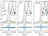 |
Fig. 1. Gaussian models (black dashed line) fitted to the observed Hβ (left), [O III] λ 5007 (center), and Hα+[NII] 6748,6584 (right) lines in the WHT/ISIS spectra of the SLCE J0925+1403. The bottom panels show residuals in the same flux units. The continuum (orange line) and the two narrow (N1, N2) and broad (B) components are shown in cyan, red, and green, respectively. The inset shows a zoomed-in image of the line wings. |
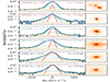 |
Fig. 2. Three-Gaussian model of [O III]5007 for a subsample observed with X-shooter. Galaxies are shown in order of increasing LyC fesc percentage. The two upper panels show galaxies classified as NLCE, the two middle panels show SLCEs, and the two bottom panels show SLCEs. The right panels show HST-COS NUV acquisition images of 1.4″ per side for each galaxy. The spectra are normalized to the peak flux and are shown in log scale to highlight low-surface-brightness wings. |
4.1. Evidence of outflows of highly turbulent ionized gas
Following Amorín et al. (2012b), we interpret the narrower emissions as resulting from the virial motions of the photoionized nebulae surrounding the brightest unresolved young star clusters, which may follow the rotation of the gaseous disk (Lofthouse et al. 2017; Bosch et al. 2019). Instead, the broad emission, which largely exceeds the velocity dispersion (∼60 km s−1) expected for rotating disks with M⋆ ≲ 1010 M⊙ (Simons et al. 2015), is ascribed to non-virial motions of high-velocity photoionized gas resulting from stellar feedback. The lack of typical AGN spectral signatures (Flury et al. 2022a) and the presence of broad components in Balmer lines and low- and high-ionization forbidden lines, strongly disfavor AGN broadening in this sample. In addition, similar objects with spatially resolved spectra show broad emissions extended to kiloparsec scales, which supports our interpretation (e.g., Bosch et al. 2019; Komarova et al. 2021)
Using a simple outflow model (Genzel et al. 2011), the broader components are consistent with a spatially unresolved outflow with vout = Δv + 2σbroad ∼ 200 − 600 km s−1. They are likely the result of the strong winds of massive star clusters in the youngest and brightest unresolved star-forming clumps, and SNe feedback. Although we cannot resolve spatially the broad emission in our spectra, we find that galaxies with a more compact and often dominant UV central clump (Fig. 2) have more complex line profiles and show broader wings, suggesting that the origin of the ionized outflows resides in the inner unresolved region of a few hundred parsecs or less.
4.2. Properties of outflowing gas from line ratios
In classic diagnostic diagrams, the excitation properties of the narrow and broad kinematic components of LCEs are consistent with line ratios driven by stellar photoionization (Fig. A.4). The narrow components show slightly higher [O III]/Hβ and lower [N II]/Hα than the broader components. However, for [O I]/Hα and [S II]/Hα we find that broad and narrow components tend to have lower ratios than normal galaxies, in line with the low [S II]/Hα found in a larger sample of LCEs using lower-resolution spectra (Wang et al. 2021). This suggests the outflow traced by the broad component may tend to optically thin conditions (Pellegrini et al. 2012) and have no significant contribution of shocks, in contrast to the higher [S II]/Hα broad components seen in more massive galaxies (e.g., luminous and ultra-luminous infrared galaxies, (U)LIRGs; Arribas et al. 2014).
In our sample, the broad component of [S II] lines is significantly fainter and has larger uncertainty than for [O III] and Hα and Hβ lines, so it should be taken with caution. With this caveat in mind, we follow Fernández et al. (2023) to derive [S II] electron densities for the individual Gaussian components. We find relatively high densities (ne ∼ 100 − 1000 cm−3), with values for the broad components that are comparable to or higher than the narrow components.
4.3. A correlation between outflow kinematics and LyC escape fraction
Revealing the nature of the broad emission in LCEs can provide new clues to how gas turbulence and stellar feedback affect Lyα and LyC photon escape. Using a small sample of GPs, Amorín et al. (2012a) found broad emission with FWZI ≳ 1000 km s−1 in recombination and forbidden nebular lines. More recent work suggests a causal connection between the complex kinematics and the high Lyα escape fractions of GPs (Orlitová et al. 2018; Bosch et al. 2019; Hogarth et al. 2020) and lower-z analogs (Herenz et al. 2016; Micheva et al. 2019; Komarova et al. 2021).
In this work we explore the above tendency using higher-resolution data for a larger sample that contains confirmed LCEs. In Fig. 3 we present a correlation between  and the intrinsic velocity dispersion (σbroad) of the Hα broad component and line asymmetry |A| (see Sect. 3) of [O III], respectively. We use the three metrics of
  obtained and discussed by Flury et al. (2022a): (i) the empirical ionizing–to–non-ionizing continuum ratio FλLyC/Fλ1100, (ii) using Hβ flux to infer the intrinsic LyC from STARBURST99 model spectra
  (Hβ), and (iii) using SED fits to the far-UV spectra to infer the intrinsic LyC
  (UV). In the upper panel of Fig. 3 the strongest leakers show a larger median velocity dispersion of σbroad > 220 km s−1 than the non-leakers, which show σbroad < 150 km s−1. Using our previous definitions (Sect. 4.1), this translates into median outflow velocities for strong leakers, weak leakers, and non-leakers of vout = 485 km s−1, 333 km s−1, and 276 km s−1, respectively. As a comparison, vout ∼ 327 km s−1 have been reported for the strong LCE Sunburst Arc (Mainali et al. 2022).
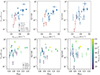 |
Fig. 3. Escape fraction traced by FλLyC/Fλ1100 (left), |


The above correlation is robust against the metric considered for the LyC escape fraction and the chosen emission line (see also Fig. A.5). This is shown in Table 1, in which we quantify the significance of the above correlations using a Kendall-τ test (Akritas & Siebert 1996). The above correlations are also evident if instead of σbroad we use the velocity widths computed from our non-parametric analysis (Fig. A.2), such as the FWZI (Fig. A.5) and w98 = v99 − v1 (i.e., the full width at the base of the line, excluding the noisy first and last 1% of the total flux contained in the blue and red wings), for which we find w98 = 640 km s−1 and w98 = 484 km s−1 for strong leakers and non-leakers, respectively.
Kendall-τ coefficients for LyC leakage and the Hα and [O III] broad-line widths.
In Fig. 3 (bottom) we note a prevalence of asymmetric [O III] profiles (|A|> 0), especially for LCEs of larger σbroad. Despite the large scatter, this relation appears evident when we compare the line profiles in Fig. A.3. Quantitively, if we consider v1, v5, and v10, which account for the velocity of the blueshifted emission line wing containing less than 1%, 5%, and 10% of the total integrated flux, respectively, we find that SLCEs have median values that are a factor of ∼1.5 larger than WLCES and NLCEs. However, no significant differences are found in the red wings (v90, v95, and v99), suggesting that the trends in Fig. 3 are driven by the escape of LyC along the same line of sight of the outflow.
4.4. Implications for LyC escape mechanisms
In our sample of galaxies, LyC photons originate in young massive stars, and a fraction of them can escape through physical processes that are still not well understood. In principle, LyC photons can either escape through density-bounded nebula or through low H I column density holes or channels carved in the ISM (e.g., Zackrisson et al. 2013; Jaskot & Oey 2013). Observations of LyC leakers have shown that the latter mechanism is largely at play (e.g., Reddy et al. 2016; Gazagnes et al. 2018; Saldana-Lopez et al. 2022; Xu et al. 2023a). However, how these optically thin channels are created is unclear. Simulations show that strong SNe feedback plays a key role in shaping the ISM and carving the holes through which LyC photons escape (e.g., Trebitsch et al. 2017; Kimm et al. 2019). In addition, intense stellar feedback injects strong turbulence in the ISM that can produce photoionized channels that favor LyC escape (Kakiichi & Gronke 2021).
We find a clear signature of turbulent ionized gas kinematics driven by stellar and SNe feedback in a sample of LCEs. The width of the broad-line emission correlates with  , providing new clues to the escaping mechanism. Assuming that LyC photons in our LCEs emerge from the youngest starbursts (≲5 Myr), radiative feedback due to strong radiation pressure in the late stages of the evolution of massive stars can create an outflowing bubble of gas surrounding dense young star clusters. On this short timescale, the first SNe explode and produce mechanical energy and momentum, and cosmic ray feedback. This is further supported by the recent study of Bait et al. (2023), who found evidence of SNe-driven non-thermal emission in the radio continuum observations of LzLCS galaxies, including 11 galaxies in our sample. In the youngest objects, however, the development of large-scale SNe-driven superwinds could be suppressed due to catastrophic cooling (Jaskot et al. 2019; Komarova et al. 2021; Oey et al. 2023). Thus, the relations we see in Fig. 3 may well be driven by radiatively driven outflows, which may carve dust-transparent ionized channels approaching density-bounded conditions (e.g., Jaskot & Oey 2013) that favor large escape fractions (Ferrara 2024).
In this scenario the broad emission-line wings of LCEs could originate from the bulk outflow near the starburst (Martin et al. 2015) and from dense pockets of highly ionized gas interacting with a high-velocity wind fluid, possibly entrained near the base of a larger-scale wind and close to the ionization source (Hayes 2023) or in the shell of the highly ionized bubble. On longer timescales (≳5 − 10 Myr), SNe feedback should take over when the LyC production from massive stars declines rapidly (e.g., Naidu et al. 2022). Outflows may have time enough to break the ionizing bubbles and produce larger cavities and holes in the ISM. Results from current models and simulations suggest that the two feedback modes could eventually operate sequentially (e.g., Kakiichi & Gronke 2021; Katz et al. 2023).
Observationally, a two-stage starburst has been proposed to explain the ionizing photon escape in some galaxies (Micheva et al. 2018). In this scenario, shocks induced by recent SNe explosions from an initial starburst episode with ages > 10 Myr may have enough time to clear out the surrounding ISM allowing the LyC photon production of a second younger starburst (< 5 Myr) to have an easier escaping path (e.g., Enders et al. 2023).
Triggered star formation in the denser shells of cold gas shaped by the mechanical feedback from a previous starburst episode has been reported in galactic and extragalactic nebulae (e.g., Egorov et al. 2023). The younger massive stars emerging from these regions can produce large amounts of ionizing photons that may escape from the nebula, as predicted by simulations (Ma et al. 2020). This scenario could be interesting to explain the observed scatter in the different relations between  and global properties (e.g., Flury et al. 2022b). Nevertheless, it is difficult to probe because the ongoing starburst generally dominates the observed nebular emission, and resolving the short timespan between two recent bursts from optical spectral synthesis is challenging, even with very high S/N spectra (Amorín et al. 2012a; Fernández et al. 2022). Future spatially resolved UV to near-IR spectroscopy will help to probe this scenario.
Finally, geometric effects have an important role in the connection between gas kinematics and the escape of ionizing photons (e.g., Zastrow et al. 2011; Bassett et al. 2019; Ramambason et al. 2020; Carr et al. 2021). LyC escape could be highly anisotropic and viewing-geometry dependent (Kim et al. 2023). The asymmetry of line profiles with a prevalence of blueshifted emission in our LCEs could indicate anisotropic leakage through favorable pencil-beam sightlines that are less affected by dust obscuration (Martin et al. 2015). We note that the stronger LCEs tend to have the most compact and least attenuated starbursts (i.e., very high SFR surface densities and βUV slopes; see also Flury et al. 2022b; Chisholm et al. 2022). This discussion will be expanded in a future study via the detailed comparison of the UV and optical line profiles.
5. Conclusions and outlook
In this work we present new high-resolution optical spectra of 6 strong ( ) and 11 weak LyC emitters (
 ), and 3 galaxies without significant LyC leakage (
 ). Using this data we performed a first kinematic analysis of resolved emission-line profiles using multicomponent Gaussian fitting.
Our results demonstrate the ubiquitous presence of broad emission-line wings (σbroad ∼ 100 − 300 km s−1), often blueshifted (Δvr ∼ 20 − 70 km s−1), tracing high-velocity emission-line components (FWZI ≳ 750 km s−1) that underlie narrower components (σnarrow ∼ 40 − 100 km s−1). The narrow emission traces HII regions, which follow the disk kinematics and are associated with young bright star-forming regions responsible for the production of the ionizing photons. The broad emission is instead interpreted as a turbulent photoionized gas tracing an unresolved outflow, likely driven by starburst feedback, namely strong radiation pressure, winds of young massive stars, and SNe.
We find a significant correlation between the intrinsic velocity dispersion and maximum line-width velocities of galaxies and their LyC escape fraction. Thus, strong LyC leakers show stronger broad components with larger line widths and a prevalence of larger asymmetries than weak leakers and non-leakers. This kinematic complexity of strong leakers contrasts with their otherwise simpler UV morphology from HST/COS imaging.
Although SNe-driven feedback should play a role in the entire galaxy sample (Bait et al. 2023), we speculate that in the stronger LCEs, the broad emission primarily emerges from the radiation pressure and strong winds of massive stars in the highly pressurized environment of extremely young and unresolved (< 250 pc) star-forming clumps that dominate the UV luminosity budget of these galaxies.
Overall, our results strongly suggest that the physical mechanisms driving the observed kinematic complexity play a significant role in the escape of ionizing photons in galaxies. This adds new observational support to predictions of models and simulations (e.g., Trebitsch et al. 2017; Kimm et al. 2019; Kakiichi & Gronke 2021), in which ongoing starbursts and their related radiative and mechanical feedback produce gas turbulence and outflows that are key in clearing channels through which ionizing radiation escapes into the intergalactic medium.
Future work will increase the number of galaxies with LyC observations at low and high redshifts, for which medium- or high-resolution spectra with ground-based spectrographs could extend this relation. Different fitting techniques and physically motivated models will also be explored (Komarova et al. 2021; Flury et al. 2023). In addition, spatially resolved high-resolution spectra are needed to identify the source of the outflow and the ionizing photons in LCEs. We find that detection of broad-line components in GPs could be indicative of LyC leakage. Features like these can be probed in reionization galaxies with the JWST/NIRSpec (e.g., Carniani et al. 2023; Xu et al. 2023b). Finally, future HST/COS high-resolution UV spectra are needed to better constrain the outflows seen in absorption and to compare Lyα and optical emission-line profiles, whereas HST optical narrowband imaging may provide additional hints for constraining the geometry of the emitting regions.
Acknowledgments
R.A. acknowledges the support of ANID FONDECYT Regular Grant 1202007 and DIDULS/ULS PTE2053851. V.F. and D.M. acknowledge support from ANID FONDECYT Postdoctoral grant 3200473 and ANID Scolarship Program 2019-21191543, respectively. J.M.V. acknowledges financial support from the State Agency for Research of the Spanish MCIU through “Center of Excellence Severo Ochoa” award to the IAA-CSIC (SEV-2017-0709) and CEX2021-001131-S and PID2022-136598NB-C32 funded by MCIN/AEI/10.13039/501100011033, and from project PID2019-107408GB-C44. N.G. and Y.I. acknowledge support from the National Academy of Sciences of Ukraine (Project No. 0121U109612). A.S.L. acknowledges support from Knut and Alice Wallenberg Foundation.
References
- Akaike, H. 1974, IEEE Trans. Automat. Control, 19, 716 [Google Scholar]
- Akritas, M. G., & Siebert, J. 1996, MNRAS, 278, 919 [NASA ADS] [CrossRef] [Google Scholar]
- Amorín, R. O., Pérez-Montero, E., & Vílchez, J. M. 2010, ApJ, 715, L128 [CrossRef] [Google Scholar]
- Amorín, R., Pérez-Montero, E., Vílchez, J. M., et al. 2012a, ApJ, 749, 185 [CrossRef] [Google Scholar]
- Amorín, R., Vílchez, J. M., Hägele, G. F., et al. 2012b, ApJ, 754, L22 [CrossRef] [Google Scholar]
- Arribas, S., Colina, L., Bellocchi, E., et al. 2014, A&A, 568, A14 [NASA ADS] [CrossRef] [EDP Sciences] [Google Scholar]
- Bait, O., Borthakur, S., Schaerer, D., et al. 2023, A&A, submitted [arXiv:2310.18817] [Google Scholar]
- Barrow, K. S. S., Robertson, B. E., Ellis, R. S., et al. 2020, ApJ, 902, L39 [NASA ADS] [CrossRef] [Google Scholar]
- Bassett, R., Ryan-Weber, E. V., Cooke, J., et al. 2019, MNRAS, 483, 5223 [Google Scholar]
- Bosch, G., Hägele, G. F., Amorín, R., et al. 2019, MNRAS, 489, 1787 [NASA ADS] [CrossRef] [Google Scholar]
- Cardamone, C., Schawinski, K., Sarzi, M., et al. 2009, MNRAS, 399, 1191 [NASA ADS] [CrossRef] [Google Scholar]
- Carniani, S., Venturi, G., Parlanti, E., et al. 2023, A&A, submitted [arXiv:2306.11801] [Google Scholar]
- Carr, C., Scarlata, C., Henry, A., et al. 2021, ApJ, 906, 104 [NASA ADS] [CrossRef] [Google Scholar]
- Chisholm, J., Orlitová, I., Schaerer, D., et al. 2017, A&A, 605, A67 [NASA ADS] [CrossRef] [EDP Sciences] [Google Scholar]
- Chisholm, J., Saldana-Lopez, A., Flury, S., et al. 2022, MNRAS, 517, 5104 [CrossRef] [Google Scholar]
- Egorov, O. V., Kreckel, K., Glover, S. C. O., et al. 2023, A&A, 678, A153 [NASA ADS] [CrossRef] [EDP Sciences] [Google Scholar]
- Enders, A. U., Bomans, D. J., & Wittje, A. 2023, A&A, 672, A11 [NASA ADS] [CrossRef] [EDP Sciences] [Google Scholar]
- Fernández, V., Terlevich, E., Díaz, A. I., et al. 2018, MNRAS, 478, 5301 [CrossRef] [Google Scholar]
- Fernández, V., Amorín, R., Pérez-Montero, E., et al. 2022, MNRAS, 511, 2515 [CrossRef] [Google Scholar]
- Fernández, V., Amorín, R., Sanchez-Janssen, R., et al. 2023, MNRAS, 520, 3576 [CrossRef] [Google Scholar]
- Ferrara, A. 2024, A&A, in press https://doi.org/10.1051/0004-6361/202348321 [NASA ADS] [CrossRef] [EDP Sciences] [Google Scholar]
- Flury, S. R., Jaskot, A. E., Ferguson, H. C., et al. 2022a, ApJS, 260, 1 [NASA ADS] [CrossRef] [Google Scholar]
- Flury, S. R., Jaskot, A. E., Ferguson, H. C., et al. 2022b, ApJ, 930, 126 [NASA ADS] [CrossRef] [Google Scholar]
- Flury, S. R., Moran, E. C., & Eleazer, M. 2023, MNRAS, 525, 4231 [NASA ADS] [CrossRef] [Google Scholar]
- Freudling, W., Romaniello, M., Bramich, D. M., et al. 2013, A&A, 559, A96 [NASA ADS] [CrossRef] [EDP Sciences] [Google Scholar]
- Gazagnes, S., Chisholm, J., Schaerer, D., et al. 2018, A&A, 616, A29 [NASA ADS] [CrossRef] [EDP Sciences] [Google Scholar]
- Genzel, R., Newman, S., Jones, T., et al. 2011, ApJ, 733, 101 [Google Scholar]
- Guseva, N. G., Izotov, Y. I., Schaerer, D., et al. 2020, MNRAS, 497, 4293 [CrossRef] [Google Scholar]
- Heckman, T. M., Borthakur, S., Overzier, R., et al. 2011, ApJ, 730, 5 [Google Scholar]
- Herenz, E. C., Gruyters, P., Orlitova, I., et al. 2016, A&A, 587, A78 [NASA ADS] [CrossRef] [EDP Sciences] [Google Scholar]
- Hayes, M. J. 2023, MNRAS, 519, L26 [Google Scholar]
- Hogarth, L., Amorín, R., Vílchez, J. M., et al. 2020, MNRAS, 494, 3541 [NASA ADS] [CrossRef] [Google Scholar]
- Izotov, Y. I., Orlitová, I., Schaerer, D., et al. 2016a, Nature, 529, 178 [Google Scholar]
- Izotov, Y. I., Schaerer, D., Thuan, T. X., et al. 2016b, MNRAS, 461, 3683 [Google Scholar]
- Izotov, Y. I., Schaerer, D., Worseck, G., et al. 2018a, MNRAS, 474, 4514 [Google Scholar]
- Izotov, Y. I., Worseck, G., Schaerer, D., et al. 2018b, MNRAS, 478, 4851 [Google Scholar]
- Jaskot, A. E., & Oey, M. S. 2013, ApJ, 766, 91 [Google Scholar]
- Jaskot, A. E., Dowd, T., Oey, M. S., et al. 2019, ApJ, 885, 96 [NASA ADS] [CrossRef] [Google Scholar]
- Kakiichi, K., & Gronke, M. 2021, ApJ, 908, 30 [CrossRef] [Google Scholar]
- Katz, H., Saxena, A., Rosdahl, J., et al. 2023, MNRAS, 518, 270 [Google Scholar]
- Kim, K., Malhotra, S., Rhoads, J. E., et al. 2020, ApJ, 893, 134 [NASA ADS] [CrossRef] [Google Scholar]
- Kim, K. J., Bayliss, M. B., Rigby, J. R., et al. 2023, ApJ, 955, L17 [NASA ADS] [CrossRef] [Google Scholar]
- Kimm, T., & Cen, R. 2014, ApJ, 788, 121 [NASA ADS] [CrossRef] [Google Scholar]
- Kimm, T., Blaizot, J., Garel, T., et al. 2019, MNRAS, 486, 2215 [Google Scholar]
- Komarova, L., Oey, M. S., Krumholz, M. R., et al. 2021, ApJ, 920, L46 [NASA ADS] [CrossRef] [Google Scholar]
- Liu, G., Zakamska, N. L., Greene, J. E., et al. 2013, MNRAS, 436, 2576 [NASA ADS] [CrossRef] [Google Scholar]
- Llerena, M., Amorín, R., Pentericci, L., et al. 2023, A&A, 676, A53 [NASA ADS] [CrossRef] [EDP Sciences] [Google Scholar]
- Lofthouse, E. K., Houghton, R. C. W., & Kaviraj, S. 2017, MNRAS, 471, 2311 [NASA ADS] [CrossRef] [Google Scholar]
- Ma, X., Hopkins, P. F., Kasen, D., et al. 2016, MNRAS, 459, 3614 [Google Scholar]
- Ma, X., Quataert, E., Wetzel, A., et al. 2020, MNRAS, 498, 2001 [Google Scholar]
- Mainali, R., Rigby, J. R., Chisholm, J., et al. 2022, ApJ, 940, 160 [NASA ADS] [CrossRef] [Google Scholar]
- Marques-Chaves, R., Schaerer, D., Álvarez-Márquez, J., et al. 2022a, MNRAS, 517, 2972 [CrossRef] [Google Scholar]
- Marques-Chaves, R., Schaerer, D., Amorín, R. O., et al. 2022b, A&A, 663, L1 [NASA ADS] [CrossRef] [EDP Sciences] [Google Scholar]
- Martin, C. L., Dijkstra, M., Henry, A., et al. 2015, ApJ, 803, 6 [Google Scholar]
- Matthee, J., Sobral, D., Hayes, M., et al. 2021, MNRAS, 505, 1382 [NASA ADS] [CrossRef] [Google Scholar]
- Micheva, G., Oey, M. S., Keenan, R. P., et al. 2018, ApJ, 867, 2 [NASA ADS] [CrossRef] [Google Scholar]
- Micheva, G., Christian Herenz, E., Roth, M. M., et al. 2019, A&A, 623, A145 [NASA ADS] [CrossRef] [EDP Sciences] [Google Scholar]
- Naidu, R. P., Matthee, J., Oesch, P. A., et al. 2022, MNRAS, 510, 4582 [CrossRef] [Google Scholar]
- Nelson, D., Pillepich, A., Springel, V., et al. 2019, MNRAS, 490, 3234 [Google Scholar]
- Newville, M., Stensitzki, T., Allen, D. B., & Ingargiola, A. 2014, https://doi.org/10.5281/zenodo.11813 [Google Scholar]
- Oey, M. S., Sawant, A. N., Danehkar, A., et al. 2023, ApJ, 958, L10 [NASA ADS] [CrossRef] [Google Scholar]
- Orlitová, I., Verhamme, A., Henry, A., et al. 2018, A&A, 616, A60 [Google Scholar]
- Pellegrini, E. W., Oey, M. S., Winkler, P. F., et al. 2012, ApJ, 755, 40 [NASA ADS] [CrossRef] [Google Scholar]
- Ramambason, L., Schaerer, D., Stasińska, G., et al. 2020, A&A, 644, A21 [NASA ADS] [CrossRef] [EDP Sciences] [Google Scholar]
- Reddy, N. A., Steidel, C. C., Pettini, M., et al. 2016, ApJ, 828, 108 [NASA ADS] [CrossRef] [Google Scholar]
- Rosdahl, J., Katz, H., Blaizot, J., et al. 2018, MNRAS, 479, 994 [NASA ADS] [Google Scholar]
- Saldana-Lopez, A., Schaerer, D., Chisholm, J., et al. 2022, A&A, 663, A59 [NASA ADS] [CrossRef] [EDP Sciences] [Google Scholar]
- Simons, R. C., Kassin, S. A., Weiner, B. J., et al. 2015, MNRAS, 452, 986 [Google Scholar]
- Trebitsch, M., Blaizot, J., Rosdahl, J., et al. 2017, MNRAS, 470, 224 [NASA ADS] [CrossRef] [Google Scholar]
- Vanzella, E., Castellano, M., Bergamini, P., et al. 2022, A&A, 659, A2 [NASA ADS] [CrossRef] [EDP Sciences] [Google Scholar]
- Wang, B., Heckman, T. M., Amorín, R., et al. 2021, ApJ, 916, 3 [NASA ADS] [CrossRef] [Google Scholar]
- Wise, J. H., & Cen, R. 2009, ApJ, 693, 984 [NASA ADS] [CrossRef] [Google Scholar]
- Xu, X., Heckman, T., Henry, A., et al. 2023a, ApJ, 948, 28 [NASA ADS] [CrossRef] [Google Scholar]
- Xu, Y., Ouchi, M., Nakajima, K., et al. 2023b, ApJ, submitted [arXiv:2310.06614] [Google Scholar]
- Zackrisson, E., Inoue, A. K., & Jensen, H. 2013, ApJ, 777, 39 [NASA ADS] [CrossRef] [Google Scholar]
- Zastrow, J., Oey, M. S., Veilleux, S., et al. 2011, ApJ, 741, L17 [NASA ADS] [CrossRef] [Google Scholar]
- Zastrow, J., Oey, M. S., Veilleux, S., et al. 2013, ApJ, 779, 76 [NASA ADS] [CrossRef] [Google Scholar]
Appendix A: Additional figures
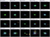 |
Fig. A.1. Sample of galaxies. SDSS-DR16 ugriz color cutouts are displayed. Galaxies are shown from top left to bottom right in order of decreasing |

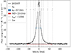 |
Fig. A.2. Illustration of the inter-percentile analysis performed by LiMe (Fernández et al. 2023, fully documented in https://lime-stable.readthedocs.io/en/latest/). Shown are the [O III] 5007 line profile of the LCE J115204+340049. The velocity percentiles vp enclosing p% of the total line integrated flux are indicated with vertical dotted lines. The red arrow line illustrates the full width at zero intensity (FWZI) computed as v100 − v0. The inset also shows values for the derived relevant quantities, including w80 (blue arrow) and the median (vmed) and peak velocity (vpeak), the latter assumed to be the systemic velocity (see Section 2). |
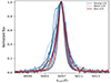 |
Fig. A.3. Superposition of normalized, continuum-subtracted, rest-frame [O III] 5007 line profiles for the galaxy sample. This illustrates the differences in asymmetry and the extent of emission line wings for SLCEs and WLCEs (blue solid and dotted line, respectively) and NLCEs (red). |
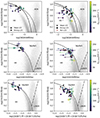 |
Fig. A.4. Classic diagnostic diagrams. Shown are gas excitation [O III]/Hβ vs. log([N II]/Hα) (top), vs. log([O I]/Hα) (middle), and vs. log([S II]/Hα) (bottom). The left and right panels show the (Izotov et al. 2016a,b, 2018a) and LzLCS (Wang et al. 2021; Flury et al. 2022a) samples (Section 2), respectively. Stars, squares, and open triangles represent integrated values. Circles indicate individual Gaussian components; the color bar gives their intrinsic velocity dispersion. |
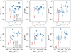 |
Fig. A.5. Escape fraction traced by FλLyC/Fλ1100 (left), |


All Tables
Kendall-τ coefficients for LyC leakage and the Hα and [O III] broad-line widths.
All Figures
|
Fig. 1. Gaussian models (black dashed line) fitted to the observed Hβ (left), [O III] λ 5007 (center), and Hα+[NII] 6748,6584 (right) lines in the WHT/ISIS spectra of the SLCE J0925+1403. The bottom panels show residuals in the same flux units. The continuum (orange line) and the two narrow (N1, N2) and broad (B) components are shown in cyan, red, and green, respectively. The inset shows a zoomed-in image of the line wings. |
| In the text | |
|
Fig. 2. Three-Gaussian model of [O III]5007 for a subsample observed with X-shooter. Galaxies are shown in order of increasing LyC fesc percentage. The two upper panels show galaxies classified as NLCE, the two middle panels show SLCEs, and the two bottom panels show SLCEs. The right panels show HST-COS NUV acquisition images of 1.4″ per side for each galaxy. The spectra are normalized to the peak flux and are shown in log scale to highlight low-surface-brightness wings. |
| In the text | |
|
Fig. 3. Escape fraction traced by FλLyC/Fλ1100 (left), |
| In the text | |
|
Fig. A.1. Sample of galaxies. SDSS-DR16 ugriz color cutouts are displayed. Galaxies are shown from top left to bottom right in order of decreasing |
| In the text | |
|
Fig. A.2. Illustration of the inter-percentile analysis performed by LiMe (Fernández et al. 2023, fully documented in https://lime-stable.readthedocs.io/en/latest/). Shown are the [O III] 5007 line profile of the LCE J115204+340049. The velocity percentiles vp enclosing p% of the total line integrated flux are indicated with vertical dotted lines. The red arrow line illustrates the full width at zero intensity (FWZI) computed as v100 − v0. The inset also shows values for the derived relevant quantities, including w80 (blue arrow) and the median (vmed) and peak velocity (vpeak), the latter assumed to be the systemic velocity (see Section 2). |
| In the text | |
|
Fig. A.3. Superposition of normalized, continuum-subtracted, rest-frame [O III] 5007 line profiles for the galaxy sample. This illustrates the differences in asymmetry and the extent of emission line wings for SLCEs and WLCEs (blue solid and dotted line, respectively) and NLCEs (red). |
| In the text | |
|
Fig. A.4. Classic diagnostic diagrams. Shown are gas excitation [O III]/Hβ vs. log([N II]/Hα) (top), vs. log([O I]/Hα) (middle), and vs. log([S II]/Hα) (bottom). The left and right panels show the (Izotov et al. 2016a,b, 2018a) and LzLCS (Wang et al. 2021; Flury et al. 2022a) samples (Section 2), respectively. Stars, squares, and open triangles represent integrated values. Circles indicate individual Gaussian components; the color bar gives their intrinsic velocity dispersion. |
| In the text | |
|
Fig. A.5. Escape fraction traced by FλLyC/Fλ1100 (left), |
| In the text | |
Current usage metrics show cumulative count of Article Views (full-text article views including HTML views, PDF and ePub downloads, according to the available data) and Abstracts Views on Vision4Press platform.
Data correspond to usage on the plateform after 2015. The current usage metrics is available 48-96 hours after online publication and is updated daily on week days.
Initial download of the metrics may take a while.