


| Issue |
A&A
Volume 711, July 2026
|
|
|---|---|---|
| Article Number | A157 | |
| Number of page(s) | 21 | |
| Section | Interstellar and circumstellar matter | |
| DOI | https://doi.org/10.1051/0004-6361/202659617 | |
| Published online | 13 July 2026 | |
B-FROST: B-Fields and star formation across scales with TRAO
CO abundances, dynamics, and relative orientations in the translucent high latitude cloud MBM12
1
Department of Physics, University of Helsinki,
Finland
2
Institut UTINAM - UMR 6213 - CNRS - Univ. Bourgogne Franche Comté,
OSU THETA, 41bis avenue de l’Observatoire,
25000
Besançon,
France
3
LPENS, Ecole Normale Supérieure, Université PSL, CNRS, Sorbonne Université, Université de Paris,
France
4
IRAP, Université de Toulouse, CNRS,
Toulouse,
France
5
Physics Department, School of Sciences and Humanities, Nazarbayev University,
Astana,
Kazakhstan
6
School of Astronomy and Space Science, Nanjing University,
Nanjing,
PR China
7
Key Laboratory of Modern Astronomy and Astrophysics (Nanjing), Ministry of Education,
Nanjing,
PR China
8
Korea Astronomy and Space Science Institute,
Daejeon,
Republic of Korea
9
Astronomy Program, Department of Physics and Astronomy, Seoul National University,
Seoul,
Korea
10
University of Science and Technology, Korea (UST),
Daejeon,
Republic of Korea
11
Shanghai Astronomical Observatory, Chinese Academy of Sciences,
Shanghai,
PR China
12
Department of Physics and Astronomy, University College London,
London,
UK
13
Institut de Ciències del Cosmos, Universitat de Barcelona,
Barcelona,
Spain
14
INAF-IAPS,
via Fosso del Cavaliere,
100,
Roma,
Italy
15
Institute of Physics and Astronomy, ELTE Eötvös Loránd University,
Budapest,
Hungary
16
Aix Marseille Univ, CNRS, CNES, LAM,
Marseille,
France
17
Institut Universitaire de France,
1 rue Descartes,
Paris,
France
18
Institute of Physics, University of Debrecen,
Hungary
★ Corresponding author: This email address is being protected from spambots. You need JavaScript enabled to view it.
Received:
26
February
2026
Accepted:
18
May
2026
Abstract
Context. On average, in our Galaxy, the star formation efficiency (SFE) is of the order of a few percent, which is lower than theoretical predictions. Detailed observational studies of individual molecular clouds may offer insight into the contributing factors to the low galactic SFE.
Aims. We investigated the high-latitude molecular cloud MBM12 as part of the B-fields and star formation across scales (B-FROST) survey with the Taeduk Radio Astronomical Observatory (TRAO) to assess why star formation activity in MBM12 is low.
Methods. We estimated N(H2) with Herschel dust emission and a dust opacity κν derived from near-infrared extinction, 21 cm HI column densities, and far-infrared emission. With 12CO and 13CO (J = 1-0) line observations, covering an area of 2.5° × 3° at 48″ resolution, we mapped the CO column density N(CO), CO-to-H2 factor X(CO), and abundance [CO/H2]. We estimated the multi-scale virial parameter αvir and constructed mass-size scaling laws of hierarchical structures with dendrograms. We computed the relative orientation between column density structures and magnetic fields using Planck observations of dust polarisation.
Results. We identified four main regions based on velocities with H2 column densities ranging from 2 × 10²⁰−1.3 × 1022 cm−2. The CO integrated line intensity, W(CO), increases linearly with N(H2), providing an average X(CO) factor close to the Galactic average. At a low N(H2), X(CO) varies below XGal due to the fall-off of collisional de-excitation in low-density gas, and above XGal due to the drop of CO abundances in poorly shielded cloud edges. The hierarchical structures follow a broken power law mass-size relation M = ARα. The values of αvir ranged from 3-60, with the smallest values at 0.1 pc scales. The mass-size relations for the structures with the lowest αvir have scaling factors, A, three times larger than those of high αvir structures, indicating external pressure one order of magnitude larger than the former. We found a transition from parallel to perpendicular relative orientations between column density structures and the magnetic field at N(H2) = 4.5 × 1021 cm−2.
Conclusions. We provide the first integrated chemical, dynamical, and magnetic field analysis of MBM12. Further investigation into the scale dependence of the mass-size relation and virial parameter can highlight the role of external pressure in regulating the star-formation efficiency.
Key words: methods: observational / ISM: abundances / ISM: clouds / ISM: kinematics and dynamics / ISM: magnetic fields / ISM: individual objects: MBM12
© The Authors 2026
 Open Access article, published by EDP Sciences, under the terms of the Creative Commons Attribution License (https://creativecommons.org/licenses/by/4.0), which permits unrestricted use, distribution, and reproduction in any medium, provided the original work is properly cited.
This article is published in open access under the Subscribe to Open model. This email address is being protected from spambots. You need JavaScript enabled to view it. to support open access publication.
1 Introduction
Molecular clouds (MCs) are among the densest and coldest large-scale structures in the interstellar medium (ISM), and they are the sites of star formation in galaxies. They evolve under the combined effects of self-gravity, turbulence, magnetic fields, radiation, and stellar feedback (Hennebelle & Falgarone 2012). The chemical evolution of MCs is closely linked to their dynamics due to comparable dynamical and chemical timescales (Dobbs et al. 2014; Chevance et al. 2023). The most commonly used tracers for large-scale (>1 pc) MC properties are carbon monoxide (CO) line emission, near-infrared (NIR) extinction, and far-infrared (FIR) dust emission, each offering complementary insights. Galactic surveys of 12CO (J = 1-0) line emission have been used for over 40 years to estimate MC masses, sizes, surface densities, densities, and velocity dispersions. These measurements underpin many of the classic MC scaling relations (Wilson et al. 1970; Solomon et al. 1987; Dame et al. 2001; Roman-Duval et al. 2010; Miville-Deschênes et al. 2017).
Near-infrared extinction is another dust-based tracer of MC structure, though the consequent column densities depend on the assumed extinction law, but NIR extinction is independent of dust temperature variations along the line of sight (Lada et al. 1994; Alves et al. 2001 ; Hasenberger et al. 2018). With the all-sky 2MASS survey, it is possible to produce ∼5′ resolution extinction maps for most of the sky (Skrutskie et al. 1997; Lombardi & Alves 2001; Lombardi 2009; Juvela & Montillaud 2016). However, the achievable resolution and dynamic range of column densities from NIR extinction are limited by stellar density.
Far-infrared dust emission is not limited by background stellar density. The Planck satellite observed the entire sky at 5′ resolution (e.g. Planck Collaboration 2014a), while the Herschel satellite allowed sub-arcminute resolution and a two-order-of-magnitude range in column density (Juvela et al. 2010; André et al. 2010; Juvela et al. 2011). Polarised dust emission also enables measurements of magnetic field orientation (Pattle et al. 2023).
Each tracer presents unique advantages and limitations. CO line emission can probe gas dynamics and chemistry, but transitions between sub-thermal, thermal, optically thick, and self-absorbing regimes complicate mass and column density estimates (e.g. Goodman et al. 2009). Extinction is among the most reliable tracers of hydrogen column density N(H) for a constant dust to gas ratio, though the extinction law may vary, and the attainable resolution is limited. Far-infrared dust emission offers high-resolution and a high dynamic range but depends on variable dust opacities and requires high-altitude or space-based observations. Magnetic field measurements are constrained by sensitivity and resolution, but they provide critical insight into the magnetohydrodynamic (MHD) processes shaping MCs (Pattle et al. 2023). A key limitation of all dust-based tracers is their inability to resolve structures along the line of sight at high-resolution (recent 3D extinction maps are addressing this problem at scales >10 pc Zucker et al. 2023).
With the advent of wide-field surveys and improved resolution, it is now possible to combine multiple tracers across large MC samples to test abundance variations, excitation conditions, and structural properties (Lombardi et al. 2006; Goodman et al. 2009; Pineda et al. 2010; Kong et al. 2015; Pety et al. 2017; Lewis et al. 2021). However, such multi-tracer analyses are rarely conducted systematically across large samples, with a few exceptions (e.g. Lewis et al. 2022; Santa-Maria et al. 2023). The B-Fields and staR formation across Scales with TRAO (BFROST) survey has completed over 2500 hours of 12CO and 13CO (J = 1-0) observations, covering nine star-forming regions across 90 square degrees (Montillaud et al., in prep.). The aim of B-FROST is to characterise the relationship between CO chemistry, multi-scale dynamics, and magnetic fields across a diverse set of environments: from high-mass star-forming regions (Monoceros OB1, W40), and feedback-dominated regions (two fields in the λ Orionis ring), to low-mass isolated clouds (MBM12,L183), and compact globules (G110-13, L1780). These sources are at distances of 100-700 pc, corresponding to spatial resolutions from ∼0.03 pc to ∼0.15 pc, respectively.
In single-tracer surveys, environmental diversity can be a weakness, introducing unknown systematics. However, because B-FROST is explicitly designed to help provide insight into how CO chemistry and dynamics interact with magnetic fields across environments, this diversity becomes a strength. Therefore, conducting in-depth studies across diverse environments allows us to identify both general trends in star-forming regions and environment-specific variations.
The most basic CO observable is the line area W(CO) = Σchan TbΔv, with Tb as the brightness temperature and Δv the channel width. The line area is related to the molecular hydrogen column density N(H2) through X(CO) = N(H2)/W(CO). For 12CO this factor has a Galactic average value of XGal = 2 × 1020 cm−2 (K km s−1)−1 (Bolatto et al. 2013). This conversion factor is essential in extragalactic studies, where high-resolution CO observations are often the only way to trace mass (e.g. Sun et al. 2018; Schinnerer & Leroy 2024; Leroy et al. 2025). The X(CO) factor is normally calculated as a means to an end (to convert CO intensity to mass), but it is rarely used as a tracer of physical properties in and of itself. It is well known that it varies on intra-cloud scales (e.g. Kong et al. 2015; Lewis et al. 2022). By definition, it is the H2 column density per CO photon, and it is therefore connected to processes of H2 and CO abundance variation, as well as CO line excitation and radiative transfer.
The CO column density N (CO) is another fundamental measure. With various assumptions, one can estimate the total CO content of an MC (see Sect. 3.2). When combined with independent measures of N(H2), one can get the projected CO abundance [CO/H2]. The CO abundance has been used to detect CO freezing onto dust grains in the coldest and densest parts of MCs (Pineda et al. 2010; Lewis et al. 2021). Although CO chemistry has been studied for decades, the relative role of UV-driven CO chemistry with dynamically induced chemistry is still an open question (van Dishoeck & Black 1988; Hennebelle & Falgarone 2012). Photodissociation region models of turbulent MCs fail to reproduce observed abundances in translucent gas (Levrier et al. 2012). Further, high-resolution maps of abundance have not yet been utilised on a large scale.
Complementary to environmental characteristics of MCs are their dynamics. Self-gravity competes with internal turbulence, magnetic tension, magnetic pressure gradients, and stellar feedback (Chevance et al. 2023). Molecular clouds are characterised by self-gravitating filamentary structures (e.g. André et al. 2010). There is some disagreement about whether the dominant mechanism shaping MC structure is self-gravity or supersonic turbulence (Vázquez-Semadeni et al. 2019; Padoan et al. 2020). There are a number of statistical tests that can be run on a position-position-velocity (PPV) cube, but projection effects and molecular abundances make direct comparison with simulations difficult (e.g. the tools in Koch et al. 2019). One controversial but easy to calculate measure of gravitational binding is the virial parameter αvir, where super- and sub-virial are relative to αvir = 2 (Bertoldi & McKee 1992), where
 (1)
(1)
with σv,st as the 1D velocity dispersion of the structure, Rst as the size, G as the gravitational constant, and Mst as the mass of the structure (Bertoldi & McKee 1992; Kauffmann et al. 2013). The case of αvir < 2 does not necessarily imply ‘bound’ and αvir > 2 ‘unbound’ (see the brief discussion in Appendix F). Yet, it can be useful when used in conjunction with other tracers and paired with a physically motivated definition of a cloud. The dendrogram algorithm by Rosolowsky et al. (2008) is a natural way to segment PPV cubes into hierarchical structures. Many analyses utilise the highest levels of dendrogram structures (e.g. Friesen & Jarvis 2024), yet only a few utilise the full multi-scale hierarchy produced by the dendrogram algorithm (Oakes et al. 2025). Tracing the scale dependence of αvir within an MC structure may yield additional insights into its stability.
Magnetic fields should not be ignored, as they increase in strength with density (Crutcher et al. 2010; Pattle et al. 2023). There has been a lot of work done mapping B-fields across scales in MCs (Arzoumanian et al. 2021; Hwang et al. 2025). In many MCs, magnetic fields transition from being parallel to column density structures at low column densities to perpendicular at high column densities, suggesting they influence cloud evolution (Soler et al. 2013; Soler 2019). Highly magnetised gas has preferential motion along field lines, leading to a perpendicular arrangement at the strong field in the high density limit (Soler et al. 2017; Suin et al. 2025). Algorithms such as FilDReaMS allow for a multi-scale consideration of B-field to column density relative orientations (Carrière et al. 2022a,b; Oers et al. 2026). Magnetic field studies are not often paired with CO virial analyses, but they may complement one another. Virial analysis with CO typically ignores magnetic fields, and relative orientation analysis cannot separate components along the line of sight.
The source we investigate as part of the B-FROST survey in this paper is the high-latitude MC MBM12 (Fig. 1). MBM12 has an estimated age of  Myr, and contains about a dozen T Tauri stars (Luhman 2001; Hogerheijde et al. 2002; Meeus et al. 2009; Kim et al. 2012). It is at a distance of
  ± 12 pc (Zucker et al. 2019), and is a well-studied MC from the MBM catalogue (Magnani et al. 1985). A previous analysis of large-scale CO mapping assumed a distance of 65 pc, and its authors concluded from a virial analysis that MBM12 is dispersing or pressure bound (Pound et al. 1990). Analysis of ammonia mapping of MBM12 concluded that it is not forming stars (Gómez et al. 2000). The MC MBM12 had an estimated mass of 1.2 × 10³ M⊙ when studied as part of the Galactic Cold Cores Herschel programme (Montillaud et al. 2015). A follow-up IRAM 30-m survey of one of the cores found rich prestellar chemistry, but did not detect deuterium or oxygen-bearing species, suggesting a quiescent core, or one at the early stages of star formation (Zhou et al. 2022). Virial analysis of a recent CO survey found αvir > 30 for most cores in the cloud (Xu et al. 2021). However, Moriarty-Schieven et al. (1997) used CO and HI observations to show that MBM12 might be pressure compressed at its southern end. So although most studies imply that MBM12 has finished forming stars and is dispersing into the environment, it may contain gas at the onset of triggered star formation.
As part of the B-FROST survey, we present an in-depth case study of MBM12. In this work, we aim to test whether MBM12 shows signs of gravitational instability despite previous indications of dispersal. We also assess how CO chemistry varies across the cloud, and whether magnetic field orientation correlates with structural or dynamical features. By combining 12CO and 13CO line emission with Herschel dust continuum data, we derive spatially resolved estimates of X(CO), N(CO), [CO/H2], and αvir across 0.05-1 pc scales. MBM12's high-latitude environment allows us to explore the role of magnetic fields and the interplay between CO chemistry and gravitational stability in a relatively pristine setting. In Section 2 we introduce the data from TRAO, Herschel and Planck observations. Then we describe our methods for estimates of H2 column density (Sect. 3.1), CO column density (Sect. 3.2), virial parameters (Sect. 3.3), and histogram of relative orientations (HROs, Sect. 3.4). In Section 4.1, we analyse the spatial distribution and probability density functions (PDFs) of N(H2), N(CO), X(CO), and [CO/H2] and compare these quantities against each other. We then look at multi-scale virial parameters (Sect. 4.2) and the histogram of relative orientation for MBM12 (Sect. 4.3). We discuss our findings in Section 5.
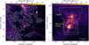 |
Fig. 1 Left: position of MBM12 relative to the galactic disk. The colour scale shows the Planck 857 GHz dust continuum, and the contours are the neutral hydrogen column density with contours at levels [1.0, 1.2, 1.4] ×1021 cm−2 from the HI4PI all sky survey (HI4PI Collaboration 2016). The beam sizes of Planck 857 GHz (orange) and H14PI (white) are shown in the bottom left. Assuming a distance of 252 pc to MBM12 and a solar height of 20 pc above the galactic plane, the distance of MBM12 from the galactic plane is shown in white. Right: zoom-in of MBM12 with the positions of T Tauri stars from Meeus et al. (2009) shown with cyan [×] markers. The observing field of view of the TRAO and Herschel observations used in this work are shown in white and yellow, respectively. A distance scale is shown in the bottom right. |
2 Observations
2.1 TRAO observations
The B-FROST survey observed MBM12 (l,b)= (159°00′00″,–34°00′00″) for 288 hours with the TRAO, operated by the Korean Astronomy and Space Science Institute (KASI)1. More details on the observations, data reduction and data quality are found in Montillaud et al. (in prep.). We observed the 12CO (J = 1-0) and the 13CO (J = 1-0) molecular lines simultaneously in on-the-fly mode with a spectral resolution of 0.2 km s−1. The angular resolution was between 46″ and 48″ for 110-115 GHz, and pointing accuracy was better than 10″(Jeong et al. 2019). We resampled all data to a grid resolution of 44″. MBM12 was mapped by scanning 0.6° × 0.6° tiles in orthogonal l and b directions. The average system temperature was 300 K and 660 K at 110 GHz and 115 GHz respectively, but we repeated the scans until the desired noise level was reached. The final map size was 2.5° × 3°. The tiles were gridded and averaged with the GILDAS CLASS2 software to make a single spectral cube for each line. We achieved a T*A sensitivity of σ12CO = 0.28 K and σ13CO = 0.13 K for most of the tiles, although some areas had a higher noise level. We converted the antenna temperature T*A to main beam temperature Tmb by dividing the antenna temperature by ηeff = 0.51 at 115 GHz and ηeff = 0.54 at 110 GHz.
2.2 Herschel and Planck observations
MBM12 was observed with the Herschel Space Observatory Spectral and Photometric Imaging REceiver (SPIRE, Griffin et al. 2010) at 250 μm, 350 μm and 500 μm as part of the Galactic Cold Cores open time programme (Juvela et al. 2010). We retrieved the MBM12 maps from the Herschel archive. The resolutions for these maps are about 18″, 25″, and 37″. The relative calibration accuracies of the Herschel SPIRE surface brightness maps are expected to be better than 4% (Bendo et al. 2013)3. We also used the Planck 353 GHz full mission data, which are available as part of the Product Release 2018 in the Planck Legacy Archive4, observed with the Planck High Frequency Instrument (HFI, Lamarre et al. 2010). We extracted from the all-sky Planck data 2° × 2° maps of the Stokes total intensity I and the Q and U parameters, which correspond to the linear polarisation components, and their uncertainties at 353 GHz centred on the Herschel maps of MBM12. We smoothed the Planck maps from an angular resolution of 4.7′ to 7′ to improve the signal-to-noise ratio. Appendix A describes our estimates of the polarisation angles.
3 Methods
3.1 H2 column density from dust emission
The Herschel SPIRE 250 μm, 350 μm and 500 μm maps were fit with modified black body (MBB) functions. Maps were colour corrected, background subtracted, and convolved to an angular resolution of 40″. The background subtraction was done by subtracting the average surface brightness of low-emission region centred on (α,δ) = (2h53m56s, +19°19′17″) with a radius of 4′ from each map. If the dust emission is optically thin, the intensity Iν can be written as:
 (2)
(2)
with Bν(Tdust) a black-body intensity with dust temperature Tdust. The values of τν and Tdust for each pixel, as well as their uncertainties, were estimated with Markov chain Monte Carlo (MCMC) runs as in Juvela et al. (2015). The H2 column density, N (H2), could then be estimated from:
 (3)
(3)
where τν is the dust optical depth at a frequency ν, κν is the dust opacity in cm2 g−1 assuming a dust-to-gas ratio of 100, mp the proton mass, and the molecular mass per H2 molecule μH2 = 2.74 (e.g. Heiderman et al. 2010). The opacity is known to vary by a factor of three between the dense and diffuse ISM (Planck Collaboration 2014a; Ysard et al. 2015; Juvela et al. 2015). Our source, MBM12, is a high-latitude cloud, so assuming a literature value of κ0 for the partly translucent ISM may be unreliable Therefore, we explored empirical calibration of κν. Calibration of κν to use with far-infrared emission requires a reference column density estimate from an independent tracer. We calibrated the 250 μm (1200 GHz) optical depth τ1200 against the K-band extinction AK (Lombardi et al. 2014; Lewis et al. 2022). For a Cardelli et al. (1989) extinction curve, RV = 3.1, and an extinction to atomic hydrogen column density conversion factor βK ≡ N(H)/AK = 1.67 × 1022 cm−2 mag−1, the dust opacity for N(H2) at 1200 GHz is given by (Lewis et al. 2022)
 (4)
(4)
where γ1200 = AK/τ1200 and fmol is the molecular gas fraction. We extracted a K-band extinction map from the iNICEST online platform (Lombardi & Alves 2001; Lombardi 2009)5. We chose a control field close to MBM12, and a smoothing full-width at half maximum of 5′, and a pixel size of 2.5′. We then convolved and reprojected the τ1200 map to the same grid and used Eq. (4) to produce the spatial variation in κ1200 (Fig. 2). We also took spatial variations in fmol into account (Appendix C). This N(H2) is then the molecular content, rather than the total hydrogen content along the line of sight. We are only considering the MC MBM12, as CO emission is emitted from inside an MC.
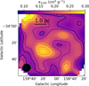 |
Fig. 2 Spatial variation in the 250 μm dust opacity in MBM12, κ1200, derived from the ratio of τ1200 and AK, accounting for the variable molecular gas fraction. The conversion assumes an extinction curve with RV = 3.1, and N(H)/Ak = 1.67 × 1022 cm−2 mag−1 (Cardelli et al. 1989; Bohlin et al. 1978; Lewis et al. 2022). Contours of κ1200 = [0.16,0.18,0.2,0.22,0.24] cm2 g−1 are overplotted. |
3.2 LTE CO column density
The method used to derive CO column densities for MBM12 is given in Montillaud et al. (in prep.). We give a brief overview of the methodology here. We derived the CO column densities, N(CO), with large-scale TRAO CO line observations. We followed Pineda et al. (2010) to estimate N(13CO). The main steps of the local thermodynamic equilibrium (LTE) estimate were estimating a Tex map from the peak Tmb of each pixel’s spectrum in the 12CO map, assuming the same Tex between 12CO and 13CO (Eq. (19) of Pineda et al. 2010). After the Tex estimate, the 13CO optical depth τ13(v) was calculated for each channel width Tmb and the Tex(Eq. (20) of Pineda et al. 2010). Lastly, 13CO column density was calculated from τ13(v) and Tex (Eq. (17) of Pineda et al. 2010). Then N(13CO) was converted to N(CO) by using the empirical isotopologue ratio with Eq. (4) of Szűcs et al. (2014), with the coefficients of model e in Table 3 of that paper. The different models consist of different initial conditions in their simulations. The choice of the model for the isotope ratio has around 20% systematic uncertainty, but it is much smaller than the uncertainty from assuming a constant isotope ratio (Szűcs et al. 2014). The assumption of the same excitation temperature between 12CO and 13CO adds uncertainty to our estimates (Padoan et al. 2000). To improve this estimate, one could either model the conversion of Tex between two isotopologues, or one could survey the cloud in the 13CO (J = 2-1) line. However, modelling the difference of Tex between the two isotopologues is non-trivial, and we did not have access to the 13CO (J = 2-1) line at 2.5° × 3° scales.
3.3 Virial analysis with CO
3.3.1 Dendrogram generation
We applied the dendrogram algorithm (Rosolowsky et al. 2008) with the astrodendro package to both CO spectral cubes. The algorithm assigns each voxel in the position-position-velocity (PPV) cube to one or more structures of connected isocontours. The structures are nested, with higher Tmb structures in PPV space always within lower Tmb structures. The trunk contains all the structures, while branches are structures with more structures within them. Structures that contain no further hierarchical structures are leaves. The minimum antenna temperature for a voxel to be considered for a structure is Tmin. The minimum number of voxels for a structure is determined by the parameter Nmin. The final parameter, ΔTmin, is the minimum Tmb difference between two peaks in PPV which could be considered as separate structures. We took Nmin = 27, Tmin = 3σrms, and ΔTmin = 3σrms, following the suggestion of Rosolowsky et al. (2008).
3.3.2 Virial parameter estimates
We estimated the virial parameter αvir for dendrogram structures assuming each structure corresponds to a sphere with mass Mst and radius Rst. We assume optically thin 13CO emission, corresponding to a direct conversion factor between the sum of Tmb of the structure and the mass Mst (Eq. (5)). The virial parameter αvir was calculated for structures at all levels with Eq. (1). We used a locally calibrated 〈X(13CO)〉 = 7.83 × 1020 cm−2 (K km s−1)−1 to convert Tmb to N(H2) (estimated in Sect. 4.1 and Fig. 5f). The benefit of using line observations with an empirical conversion from Tmb to N(H) to estimate αvir is that velocity components can be considered individually, under the assumption that each velocity component corresponds to a respective gas clump. Separating structures into a dendrogram avoids spurious increases in σv,st due to multiple velocity components along the line of sight. The mass estimate from the spectral cube was calculated as (Ladjelate et al. 2020)
 (5)
(5)
with δApixel the area of a single pixel, mH the mass of a hydrogen atom and Δv = 0.2 km s−1 the channel width. The mass of larger hierarchical structure includes the mass of that structure’s smaller scales. The pixel area δApixel = spixel,l spixel,b d2 with spixel referring to the pixel scale and d the distance to MBM12. The radius Rst was estimated as
 (6)
(6)
with A = Ppixels δApixel as the total pixel area. The velocity dispersion per pixel, σv,pixel, was calculated with
 (7)
(7)
with Ti the antenna temperature in K, vi the velocity of a channel i, ῡthe intensity-weighted mean velocity for the structure. The velocity dispersion σv,st was then the unweighted average of σv,pixel for all sky pixels. The largest systematic uncertainties in our estimate of αvir are spatial variation in X(CO), structure morphology, and distance. The 〈X(CO)〉 we use is the mean for MBM12; for low-density regions the true X(CO) can be significantly higher. The use of a constant X(CO) may underestimate the mass in low-density regions. Compared to the flux-weighted size from Rosolowsky et al. (2008), our estimate gives larger αvir as we use the total area for the radius. These considerations suggest that our estimates of αvir are upper limits (while αvir further neglects external pressure and magnetic fields, Ballesteros-Paredes 2006). However, we point out that our use of a calibrated X(CO) from κν-calibrated N(H2) reduces the uncertainty on the observed value of αvir significantly compared to assuming a X(CO) value from the literature. The distance we adopt has an uncertainty of 10%, which is systematic across the cloud, and so the uncertainty from distance is likely smaller than that from X(CO) and morphology.
3.4 Histogram of relative orientations
We applied FilDReaMS (Filament Detection and Reconstruction at Multiple Scales; Carrière et al. 2022a) to the Herschel dust column density maps of MBM12 described in Sect. 3.1. FilDReaMS is designed to detect elongated structures, which we will call filaments hereafter, in an image, and provides information on their widths, their orientations and the robustness of the detection. FilDReaMS uses a model template that has the shape of a rectangular bar (referred to as the model bar) defined by its length Lb, width Wb and aspect ratio rb = Lb/Wb. We adopt rb = 3 (Panopoulou et al. 2014; Arzoumanian et al. 2019; Carrière et al. 2022b), and we consider values of Wb spanning the range [(Wb)min, (Wb)max], with (Wb)min = 5 pix and (Wb)max = 29 pix equal to the broadest structure detected in the map. The orientation angle of the model bar, ψb, is defined in the range [−90°, +90°] and follows the IAU convention (Appendix A). For each value of Wb, FilDReaMS filters out structures broader than Wb and converts the resulting image into a binary map. At each pixel i of the binary map, FilDReaMS retrieves the orientation angle of the model bar that best matches the map, (ψb)i and computes the corresponding significance, Si, which compares the detected filament to an ideal case (see Carrière et al. 2022a for more details). If Si > 1, FilDReaMS confirms the detection of a filament with orientation angle (ψf)i = (ψb)i. Once all the pixels have been treated, FilDReaMS creates a filament mask by multiplying the above binary map with a model bar mask formed by the model bars of all the detected filaments. This filament mask is then applied to the initial image to reconstruct the physical network of detected filaments of bar width Wb with their true shapes. In case a given pixel belongs to two or more filaments, the filament orientation angle assigned to that pixel is the orientation angle of the most significant filament detected. This process is repeated over the entire range of Wb , leading to filamentary networks of different size scales.
4 Results
We identified four main regions separated by velocities in MBM12: the Horseshoe, the Bow, North Compact, and North Diffuse (Figs. 4 and 10). Figure 3 shows the mean spectra of the field. These maps were generated with emission Tmb > 5σrms. The Horseshoe is an isolated region around −6 km s−1. The Bow and North Compact are connected in emission in 12CO but not in 13CO at around −2 km s−1. North Diffuse consists of clumpy emission at > 1 km s−1.
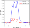 |
Fig. 3 Mean spectra over the entire MBM12 field. The velocities of each peak are indicated. |
4.1 Environmental variation
For MBM12, we show the relations between N (H2), N(CO), X(CO) and [CO/H2], and their spatial distributions and PDFs. Figure 5 shows a comparison of most of these quantities to each other. Figs. 6-9 show their spatial distributions and PDFs.
The dust-opacity-calibrated N(H2) maps of MBM12 range from N(H2) = 2 × 1020 cm−2 to 1.3 × 1022 cm−2. We generated a N(H2) probability density function (PDF) (Fig. 6). The PDF shows multiple bumps, which may be the result of the superposition of several independent column density distributions in the field.
We calculate X(12CO) and X(13CO) for the southern half of MBM12, by reprojecting the 40″ Herschel N(H2) map to the TRAO CO integrated intensity maps at 44″ resolution (Fig. 7). The morphology of X(CO) differs between the two isotopologues. In 12CO, the distribution is continuous, while in 13CO the Horseshoe is spatially disconnected from the Bow. The PDFs of X(12CO) and X(13CO) in Fig. 7 c show double-peaked distributions connected by a powerlaw. We decompose the X(CO) PDFs into a lognormal at the peak with a truncated power law. The fitting equations and results of the fit are given in Appendix E. The combination of these distributions well described the X(CO) PDFs, except an excess at X(12CO) = 10 XGal and X(13CO) = 40 XGal. Lognormal PDFs with deviations for X(CO) have been seen in 8.6′ resolution maps by Lewis et al. (2022, Appendix B). We consider physical explanations for the X(CO) PDF in Sect. 5.2.
The N(CO) varies in MBM12 from 1 × 1016 cm−2 up to 1 × 1018 cm−2 (Fig. 8). The distribution of N(CO) shows filamentary structure in the Horseshoe. In North Compact, there are some peaks, but N (CO) is relatively constant throughout the structure. The abundances [CO/H2] in MBM12 have an average of 5.9 × 10⁻⁵. The spatial distributions of the [CO/H2] have some interesting variation. At the centre of the Horseshoe, the abundances are between 4 × 10⁻⁵−1 × 10⁻⁴, with a clumpy spatial distribution. The northern islands in the Bow show centrally peaked [CO/H2] (Fig. 9). The abundances are lognormal, centred at the average abundance. The abundance shows a power-law tail at the lower end.
We compared our multi-tracer observables in Fig. 5. Three main features are (i) the quasi-linear dependence of N(CO) with N(H2 ) (panel d), leading to an average uniform CO abundance [CO/H2]=5.9×10−5. (ii) At low N(H2) (panel e), the two large excursions of W(12CO) below and above the average quasi-linear increase of W(12CO) with N(H2), corresponding to 〈X(12CO)〉 = XGal. These 1-dex excursions are responsible for the shape of the X(12CO) distribution with N(H2) (panel j). The former, at the origin of the rise of X(12CO) above XGal at N(H2) below 1.5 ×1021 cm−2, is due to the drop of the CO abundance in the least UV shielded layers, while the latter, at the origin of all the X(12CO) values below XGal, traces the fall-off of collisional de-excitation in low-density gas. (iii) The quasi-linear increase of W(13CO) with N(H2) (panel f) leading to a 13CO integrated intensity close to four times weaker than that of12CO, a result in agreement with early galactic CO and 13CO line surveys that found that 12CO lines are about five times brighter than 13CO lines (Stark et al. 1983).
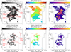 |
Fig. 4 Integrated intensity (a and d), intensity weighted mean velocity (b and e), and intensity weighted velocity dispersion (c and f) for 12CO (top) and 13CO (bottom) for MBM12 as observed with TRAO. The sub-regions of MBM12 referenced in the text are labelled in red. |
4.2 Multi-scale dynamics
4.2.1 How to interpret dendrograms
The dendrogram algorithm is a useful way of segmenting PPV cubes into hierarchical structures. Our use of dendrograms assumes each voxel in PPV corresponds to a mass proportional to the voxel’s Tmb(Rosolowsky et al. 2008). From Eq. (1) and the dendrogram algorithm, some considerations can be drawn. Higher in the hierarchy, the structures become smaller and have a higher average Tmb. Therefore, one would generally expect αvir to decrease as one moves up the dendrogram hierarchy. A similar pattern should be expected for velocity dispersion. Therefore, looking only at the leaves of a dendrogram will systematically underestimate αvir, as one ignores the pressure, shear and gravitational effects of the larger parent structure on αvir (Ballesteros-Paredes 2006). Therefore, it is helpful to look at the full hierarchy of αvir estimates. Virial parameters are calculated per structure, and are therefore difficult to visualise spatially. We produced a plot where we layer the contours of the structures, starting from the lowest hierarchical structure (i.e. the largest structure spatially). The contour is coloured by the value of the respective variable, either VLSR or αvir. We then successively layer the sub-structures on top of the largest structures to produce a two-dimensional visualisation. This works well for simpler dendrograms, such as 13CO in MBM12 (Fig. 10). We colour the dendrogram tree diagrams with VLSR and αvir, and annotated the respective sub-structures (panels c and d of Fig. 10). Virial parameters alone are not conclusive indicators of gravitational collapse, as they measure energy balance rather than stability. (Ballesteros-Paredes 2006; Offner et al. 2022; Chevance et al. 2023).
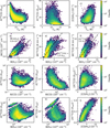 |
Fig. 5 Comparison of H2 and CO quantities observed in MBM12 with Herschel and TRAO. We compare N(H2) with CO linewidths W(CO), X-factors X(CO), 12CO excitation temperature Tex, CO column density N(CO)lte, and CO abundances [CO/H2]lte. Panels a)-c) and d)-l) have different colour scales. Panels d)-f) have linear fits shown in black lines, with the slope annotated on the respective panel. The linear striations at low N(H2) in panels j) and k) are artefacts of the sigma clipping in the W(CO) estimates. |
4.2.2 Hierarchical structure in MBM12
The 13CO emission is separated into the North Diffuse, Bow, North-Compact and Horseshoe subregions (Fig. 10). The North Diffuse subregion has a ring shape in the north of MBM12, with most structures having αvir > 4 (also seen in Pound et al. 1990). The North Diffuse region has the same velocity as the small northern clumps at VLSR ∼ 4 km s−1.
The Bow subregion has two components in 13CO, east at VLSR ~ −1 km s−1 and west at −2.5 km s−1. This subregion is also detected with Herschel. The eastern Bow at −1 km s−1 is likely denser than the western Bow, with αvir ≲ 2.5, and thin layers of large X(13CO) (middle panel of Fig. 7). The western Bow has two islands, the most western island with αvir > 5, and an eastern island with αvir ∼ 2. The western Bow has thicker layers of large X(13CO) (middle panel of Fig. 7) than the eastern Bow.
The North Compact subregion has complex hierarchical structure. It was not covered with Herschel. It has some substructures with αvir > 5 (panel d of Fig. 10), but the whole structure has αvir ∼ 3. The region has the largest N(CO) in the north of MBM12 (Fig. 8) but is not strongly centrally peaked. There are single structures in this subregion (Fig. 11) with αvir < 2, but most of this structure has αvir > 2.
The Horseshoe, at VLSR = −5.5 km s−1 has the most complex hierarchical structure in MBM12. Some structures at the southern part of the Horseshoe have αvir > 5 (Fig. 10b). Some of these may be fore- or background clumps, as they are also at different velocities. The Horseshoe has the largest average N(H2) in MBM12 and has αvir ∼ 3.
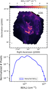 |
Fig. 6 Top: opacity-calibrated N(H2) map from Herschel observations. Bottom: dust-opacity-calibrated N(H2) PDF with Herschel for MBM12. The Herschel map covers only the southern half of MBM12. |
4.2.3 Scale dependence of αvir
We examine the interdependence of Mst and αvir on Rst for the largest structures identified in the 13CO dendrogram (Fig. 10c). We fitted a broken power law to the masses Mst and radii Rst of 13CO dendrogram structures in MBM12. The functional form is
 (8)
(8)
where i = 1 if Rst < Rbreak and i = 2 if Rst > Rbreak. The best fit parameters with uncertainties are shown in Table 1. To ensure continuity between the two power laws, from Eq. (8) the breakpoint R′break can be calculated directly:
 (9)
(9)
From the dendrogram we take trunk-level structures that have more than eleven sub-structures. Spatial investigation reveals that these structures are the Horseshoe, North Compact, eastern Bow, western Bow, southern North Diffuse, and eastern North Diffuse. We then plot the mass-size relation normalised by R2st, and the surface density dependence of αvir for all hierarchical structures (Fig. 11). Note that these data points are not independent, as they share voxels in PPV. Therefore we are rather estimating the slope of the change in mass with radius, comparable to the differential virial analysis of Krumholz et al. (2025). We found correlations between mass and radius, that are best described by a broken power laws (Fig. 11a). Table 1 show the scaling parameters Ai, power law slopes αi and break points Rbreak for all the substructures. The large scale (Rst > Rbreak) indices were close to M ∝ R2 for the Horseshoe and eastern Bow with α2 = 1.91 ± 0.02 and α = 1.92 ± 0.03 respectively. For the other subregions, the outer power law index is sub-Larson, with α2 < 1.5. The outer scaling factor A2 varies between 54169, with the largest value at the Horseshoe, and the smallest at North Diffuse subregions. However, the power law index is super-Larson for all low-mass subregions in the inner power law, with α1 > 2, and the statistically significant scaling factors A1 varying between 50−215. The virial parameter is increasing with decreasing Σst. The North Compact is the only region which contained αvir < 2 structures. However, αvir has some variation depending on the scale at which the structure is analysed. Many of the smallest scale structures in the Horseshoe and North Compact have large αvir > 2. The other structures have αvir ∼ 8 at parsec scales (Fig. 11 b), with variability in αvir towards smaller scales. No structures in eastern Bow, western Bow, southern North Diffuse, eastern North Diffuse have αvir ∼ 2 at any scale.
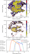 |
Fig. 7 Ratio of N(H2) and CO line area for 12CO and 13CO ground state rotational transitions in the southern half of MBM12. The figures are in units of XGal = 2 × 1020 cm−2 (K km s−1)−1. The beam size and linear scale are shown at the bottom left and right respectively. Contours of N(H2) are shown in red at levels of [1, 2, 5, 8, 10] × 1021 cm−2. The bottom panel shows the PDFs of X(12CO) and X(13CO). |
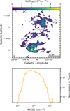 |
Fig. 8 Carbon monoxide column density N(CO) for MBM12, derived from TRAO 12CO and 13CO (J = 1-0) observations. The map shown on the top was estimated with standard LTE assumptions to derive N(13CO) and converted to total N(CO) with the isotopologue ratio function from Szűcs et al. (2014). The bottom panel shows the PDF for the N(CO) map. |
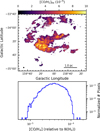 |
Fig. 9 Map of CO abundance relative to H2 column densities in the southern part of MBM12. The top panel shows N(CO) estimated from LTE assumptions. The bottom panel shows the abundance PDF. |
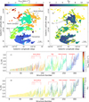 |
Fig. 10 Hierarchical structure and virial estimates for MBM12 with 13CO (J = 1-0) observations with the TRAO. Panel a: centre velocities for dendrogram structures. The plot was made by plotting the largest-scale structures first with a single colour corresponding to their Vcen, and then the smaller-scale structures have been plotted on top. Panel b: virial parameter estimates for dendrogram structures. The plot was made in the same way as panel a, but with the colour defined by the value of αvir. Panel c: tree diagram for 13CO observations of MBM12. The tree diagram is coloured according to the value of Vcen for the structure with the same colour scale as panel a. The structures with the four largest-scales are shown in red. Panel d: tree diagram for αvir estimated with the 13CO observations of MBM12. The tree diagram is coloured according to αvir with the same colour scale as panel b. |
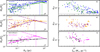 |
Fig. 11 Scale dependence of 13CO dendrogram structures in MBM12. The colours are for the Horseshoe (blue), North Compact (green), eastern Bow (yellow), western Bow (purple), southern North Diffuse (black), and eastern North Diffuse (grey). Broken power law fits are also shown, with the respective fit values in Table 1. Vertical lines indicate the power law breaking point. The vertical axis in panels a-c (Mst/R2st) is in units of solar mass per square parsec. |
4.3 Histograms of relative orientations
We examine the relative orientation between N(H2) structures and the plane-of-sky magnetic field BPoS. Figure 12 summarises our histogram of relative orientation analysis in MBM12. The top left panel shows the Herschel N(H2) map, from which networks of filaments were extracted. These networks are shown in the top middle and top right panels, with the largest-Wb and smallest- Wb filaments per pixel shown. These figures reveal very thin and low-N(H2) striations around the Horseshoe and Bow subregions. The Horseshoe has significantly thicker filaments than the Bow, with bar widths ∼0.6 pc, with a finer, continuous structure, while the Bow appears more disconnected, with bar widths of ∼0.4 pc. The middle row of Fig. 12 shows maps of the relative orientation between filaments and BPoS for the smallest-Wb filaments (left panel), largest-Wb filaments (right panel), and most significant filaments across all Wb (centre panel). The bottom row of Fig. 12 shows the histograms of relative orientations as a function of N(H2) for the same sets of filaments. At small scales, most filaments are roughly parallel to BPoS at low N(H2), with |ψf - ψb| ≲ 35° for NH2 ≤ 4.5 × 1021 cm−2, while high-N(H2) filaments have more random orientations, with a small preference towards −45°. The situation is clearer for the most significant and largest-Wb filaments. Similarly, most filaments at low-N(H2) are roughly parallel to BPoS while the high-N(H2) filaments, which correspond to the Horseshoe, shows that the northern part is mostly parallel to BPoS and the southern part is roughly perpendicular to BPoS. The HROs in MBM12 seem to indicate that at low-N(H2) filaments tend to be smaller and oriented parallel to the magnetic field. As the N(H2) increases, the filament size also increases, and these large scale filaments are either parallel or perpendicular to the magnetic field. At high N(H2), structures are located in the southern part of the Horseshoe, perpendicular to the magnetic field, where both the large scale filaments are co-spatial in the plane of the sky.
5 Discussion
5.1 Dust opacity variation and N(H2) estimation
The dust opacity κν is a function of various dust properties (size distribution, chemical composition, and structure). Dust models can predict κν among other things (e.g. Hensley & Draine 2023; Ysard et al. 2024). It is known that the far-infrared dust opacity varies in the diffuse ISM, with less pronounced variations in NIR extinction (Planck Collaboration 2014b; Reach et al. 2015; Nguyen et al. 2018). Between the diffuse ISM and MCs, there is a factor of three change in the ratio of the 250 μm and NIR opacities (Juvela et al. 2015). Empirical κν calibration is important as column density estimates propagate into mass, density and abundance estimates. We summarise some methods for estimating κ1200 in Table 2 (see Appendix D). We recommend the κν calibration method of Lewis et al. (2022) with NIR extinction. Even if NIR extinction maps do not have high-resolution, they can give a cloud averaged κν, or spatial variation in some cases that is better than assuming a constant from literature. The NIR extinction to column density ratio is not necessarily constant if RV varies, but the empirical models of Hensley & Draine (2023) can be used to quantify the uncertainty of Rv. Informed use of κν would remove bias in masses and chemical abundances in diverse star forming environments.
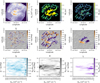 |
Fig. 12 Top left: MBM12 H2 column density map. Top middle: Network of filaments reconstructed with FilDReaMS, with the largest bar width, Wb, per pixel shown. Top right: same network of filaments with the smallest Wb per pixel shown. Middle left, middle, and right: Map of the relative orientation for the smallest Wb filaments, most significant filaments across Wb, and largest Wb filaments, respectively. BPoS orientation is visualised using line integral convolution in grayscale in the background. Bottom left, medium, and right: histograms of relative orientations as a function of N(H2) for the smallest Wb filaments, most significant filaments across Wb, and largest Wb filaments respectively. |
Summary of κ1200 estimating strategies and the consequent values.
5.2 Intra-cloud X(CO) variations
The X(CO) factor is a measure of H2 molecules per CO emission. On theoretical grounds we expect it to be affected by CO abundances, H2 kinetic temperature, H2 density, dust temperature and the surrounding radiation field (Shetty et al. 2011; Lewis et al. 2021). Molecular H2 and CO are photodissociated in the interstellar radiation field if shielding is too weak (van Dishoeck & Black 1988; Gong et al. 2018). Shielding can occur due to self-shielding, shielding by other molecules or attenuation by dust (van Dishoeck & Black 1988). Molecular hydrogen forms at low densities (>30 cm−3) with efficient self shielding, while CO requires dust to attenuate the radiation and therefore forms at hydrogen densities >100 cm−3 (van Dishoeck & Black 1988; Glover et al. 2010; Gong et al. 2018). In these intermediate densities 30-100 cm−3 is CO dark gas, which would lead one to expect X(CO) → ∞ as CO starts to form at the outer edges of MCs. However observations of diffuse clouds have rather found X(CO) ≤ XGal (Liszt et al. 2010; Liszt & Pety 2012). This can be explained by low collisional de-excitation for CO at low densities, where CO is more effective per H2 molecule at emission (Hennebelle & Falgarone 2012). The variance of the X(CO) factor is also very high in diffuse regions, where nH2 < 400 cm−3 (Shetty et al. 2011). Deeper into the cloud, where AV is between 1 and 2 mag, the dust shields the interstellar radiation field for the formation of CO, X(CO) exponentially decreases (Shetty et al. 2011; Szűcs et al. 2016). However, at the largest densities, the lines may self-absorb, or CO is frozen onto dust grains, which then increases X(CO) again (Pineda et al. 2010; Szűcs et al. 2016). We see these regimes in Figs. 5j and k. For N(H2) below 1021 cm−2, we have high X(12CO) values, but also many where X(12CO) < XGal. The mean value of X(12CO) was very close to the galactic average recommended by Bolatto et al. (2013). Our estimate is twice the value of ≈0.5XGal surrounding MBM12 from Remy et al. (2017). In Perseus X(12CO) was measured as 0.5-1.5XGal (Pineda et al. 2008). The relationship between X(CO) and N(H2) has been investigated theoretically and through observations of the California MC as well (Kong et al. 2015; Szűcs et al. 2016; Lewis et al. 2021). Magnani et al. (1988) calculated X(CO) for various high-latitude clouds (excluding MBM12) and found an average value of X(CO) = 3.2 ± 0.6 XGal for their full sample, or 1.6 XGal if they excluded some dark clouds. They also estimated abundances of 4-12 × 10−5 which is closer to our estimate of MBM12 than to the average Milky Way value. Cotten & Magnani (2013) estimated X(CO) = 0.65 XGal for MBM 40. In MBM16, X(CO) = 3.6 XGal and in MBM40 X(CO) = 1.3 XGal (Magnani et al. 1998). The X(CO) PDFs possibly encode this chemical behaviour (Fig. 7). Close to the average value of X(CO) the PDF was lognormal, with a similar standard deviation of around 1.4 XGal. In App E, we use the statistical behaviour of the X(CO) PDF to visualise the physical transitions in MBM12 Fig. E.1. If other MCs show similar lognormal and powerlaw behaviour in their X(CO) PDFs, the PDF properties can be used as a measure of chemistry and excitation. Most works only focus on X(CO) as a conversion factor for mass. However, our 44″ investigation of X(CO) implies that it may be a useful probe of MC substructure in its own right. Radiative transfer modelling of the X(CO) PDFs physical dependencies combined with estimates from more sources may reveal if X(CO) PDFs have any diagnostic potential.
5.3 CO abundances
The highest CO column densities in MBM12 was 1 × 1018 cm−2. The high column densities are associated with the Horseshoe and North Compact (Fig. 8). The measured N(CO) for MBM12 of a few 1017 is higher than any MBM clouds in the sample of van Dishoeck et al. (1991). The mean [CO/H2] of 5.91 × 10⁻⁵ of MBM12 is lower than the canonical 10−4 in Milky Way clouds such as Taurus and Orion B (Pineda et al. 2010; Bolatto et al. 2013; Roueff et al. 2021). Low abundances like this have been observed before (Burgh et al. 2007; Liu et al. 2013; Luo et al. 2023). The methodological assumptions that go into abundance calculations (κν for N(H2), constant Tex, isotope ratio, LTE only vs non-LTE) make precise comparison with other works difficult. In the case of Taurus Pineda et al. (2010), assumed a constant isotope ratio of 69, which increases their N (CO) estimate by up to 70%, compared to our use of a variable isotope ratio (Szűcs et al. 2014). Variable isotope ratio would also change the shape of the N(CO) and [CO/H2] PDFs. The environmental differences between Taurus and MBM12 play a role in the abundance differences.
5.4 Virial analysis in MBM12
We used virial analysis as one tool among many for assessing virial equilibrium. In Appendix F we discuss some of the historical ambiguities in the interpretation of αvir. We find αvir ≳ 3 for all regions in MBM12. In all cases, αvir did not vary significantly with scale. The scale independence of αvir has also been seen in other regions, including Serpens South and NGC 253 (Luo et al. 2024; Friesen & Jarvis 2024; Oakes et al. 2025). Scale independent αvir is expected for structures. If the structures follow Larson’s laws,  and
and  , then from Eq. (1)
  . The scaling factors in front of the mass-size relations (Fig. 11) in the Horseshoe are up to three times higher than that of the northern regions. The
  and
and  hierarchy is the locus of the gravitational instability threshold of self-gravitating polytropes of increasing temperature immersed in a common pressure reservoir Pext. The structures of this hierarchy are the result of fragmentation of the larger scales, which occurs prior to collapse, and behave as a N -body system in virial equilibrium (Chieze 1987). The interesting point here is that the pre-factor of the mass-size relation is proportional to
  which shows that the external pressure of the structures of lowest αvir is about 10 times larger than that of the structures of largest αvir. For a turbulent core with a constant surface density, an increased internal pressure (which is related to the external pressure) should increase αvir (McKee & Holliman 1999; McKee & Tan 2003). We do observe that the smaller scale structures Rst < Rbreak, with larger mass-size coefficients have larger virial parameters (Fig. 11d). Additional investigation will be required into the role of pressure in the scale dependent behaviour of αvir, such as the analysis proposed by Krumholz et al. (2025).
5.5 Magnetic fields and gravitational stability in MBM12
From the analysis of ideal MHD equations, Soler & Hennebelle (2017) showed that perpendicular and parallel alignments between magnetic field orientations and column density structures are attractors in the equations of motion. In strongly magnetised (plasma β ∼ 0.1) gas the transition between these two attractor modes are induced through convergent flows where ∇ ∙ u < 0 (Soler et al. 2013; Soler & Hennebelle 2017). Convergent flows can either be large scale flows or self-gravity, which dominates magnetic pressure gradients in MCs (Chen et al. 2016). Observational studies of ten Gould Belt regions with Planck dust emission and polarisation measurements found a transition column density  (Planck Collaboration 2016). This transition N(H) is close to the Nc→pl (H) = 1021 cm−2 where the upper limits of magnetic field strengths from Zeeman measurements transition from constant to power law (Crutcher 2012; Soler & Hennebelle 2017). The connection between the N||→⊥ to Nc→pl(H) may indicate a shared mechanism of super-critical filaments between these two transitions. However, this interpretation is weakened by the large scatter in measured N∥→⊥(H), which ranges from 2 × 1021 cm−2 to 23 × 1021 cm−2, or many clouds not displaying a transition at all (Planck Collaboration 2016; Soler et al. 2017; Carrière et al. 2022b). MBM12 displays a transition column density of N∥→⊥(H2) ~ 4.5 × 1021 cm−2 and α ≈ 3 in the Horseshoe. Our virial parameter ignores contributions from internal magnetic pressure or external thermal pressure, which brings up the question of whether the magnetic field is supporting MBM12 from collapse. For a single source, a parallel to perpendicular transition is difficult to interpret (Sect. 6.1.3 of Pattle et al. 2023). The presence of the relative orientation transition indicates the presence of strong magnetic fields β < 1, convergent velocity flows and possibly super-Alfvénic gas motions. The south of MBM12 Horseshoe would therefore be a candidate for higher resolution kinematic follow-up, to assess whether there are signs of infall or gravitational collapse.
6 Conclusion
We report large-scale 12CO and 13CO (J = 1-0) line observations of MBM12 with the TRAO radio telescope combined with Herschel and Planck column density estimates. For the first time in MBM12, we combined an analysis of molecular gas properties (N(H2), X(CO), N(CO), [CO/H2]), dynamics (multi-scale virial parameters αvir), and magnetic fields (with histogram of relative orientations):
We estimated the spatial variation in the molecular gas fraction and 1200 GHz dust opacity, with 〈κ1200〉 = (192 ± 7) × 10−3 cm2 g−1, resulting in column densities that range from 2 × 1020 cm−2 to 1.3 × 1022 cm−2;
The average CO-to-H2 conversion factors were X(12CO) = 2 × 1020 cm−2 (K km s−1)−1 and X(13CO) = 7.8 × 1020 cm−2 (K km s−1)−1 with significant variation across the field. The average X(12CO) value in MBM12 is equal to the galactic average. We decomposed the X(CO) PDFs into lognormal and power law components, with the power law slopes of X(12CO) = −1.21 ± 0.03 and X(13CO) = −0.78 ± 0.04. Future work will investigate the parameters which influence the statistical intracloud behaviour of X(CO);
We estimated the CO column density N (CO), and the CO abundances [CO/H2]. We incorporated variable 12CO/13CO isotope ratios calibrated by simulations. We measured N(CO) ranging from 1 × 1016 cm−2 to 1 × 1018 cm−2. The abundances [CO/H2] ranged from 0.9 × 10⁻⁵ to 1 × 10⁻⁴ with an average of 5.9×10⁻⁵;
We used dendrograms to calculate multi-scale virial parameters αvir for MBM12. For the Horseshoe and North Compact subregions, for most structures αvir ≃ 3 at scales of 0.05− 1 pc with masses scaling M ≃ R2 and Larson scaling σv ≃ R0.5. On the other hand for the North Diffuse and Bow regions αvir ≃ 8 at scales of 0.05− 1 pc. The Horseshoe has a mass-radius scaling coefficient three times larger than the other subregions, indicating an order of magnitude stronger external pressure on the Horseshoe, compared to the other subregions. Scale dependent αvir measurements can highlight the role of external pressure in regulating star formation MCs;
We estimated the histogram of relative orientations in MBM12, and found column density structures parallel to the magnetic field orientation for N(H2) < 4.5 × 1021 cm−2, and some perpendicular structures thereafter. Perpendicular structures were only detected in the south of the Horseshoe subregion, and may indicate the presence of strong magnetic fields and convergent velocity flows.
Our first case study of MBM12 in the B-FROST survey highlights the complementary value of tracing environment, dynamics, and magnetic fields. We also stress the value of empirical κν calibration for H2 column densities and assumptions about LTE and isotope ratios for CO column densities. The multi-tracer approach in MBM12 enables comparative studies of low- vs high-mass star formation under varying conditions of turbulence, feedback, and magnetisation in large scale MC surveys.
Data availability
Data products are available at the CDS via https://cdsarc.cds.unistra.fr/viz-bin/cat/J/A+A/711/A157. Included are the 12CO and 13CO (J = 1-0) cubes, integrated intensity and mean velocity for both lines, LTE N(CO) map and the local κν calibrated N(H2) map.
Acknowledgements
We thank Quentin Remy for supplying the opacity maps of anti-centre clouds. JMV and MJ acknowledge support from the Academy of Finland grant No. 348342. EM is funded by the University of Helsinki doctoral school in particle physics and universe sciences (PAPU). VMP acknowledges financial support by the grant PID2020-115892GB-I00, funded by MCIN/AEI/10.13039/501100011033 and by the grant CEX2019-000918-M funded by MCIN/AEI/10.13039/501100011033. VMP gratefully acknowledges also financial support from the European Research Council via the ERC Synergy Grant ‘ECOGAL’ (project ID 855130). DA acknowledges NU FDCRGP No201223FD8821. We acknowledge the use of data provided by the Centre d’Analyse de Données Etendues (CADE), a service ofIRAP-UPS/CNRS (http://cade.irap.omp.eu, Paradis et al. 2012). C.W.L. is supported by the Basic Science Research Program through the NRF funded by the Ministry of Education, Science and Technology (grant No. NRF- 2019R1A2C1010851) and by the Korea Astronomy and Space Science Institute grant funded by the Korea government (MSIT; project No. 2025-1-841-02). This research made use of astro-dendro, a Python package to compute dendrograms of Astronomical data (http://www.dendrograms.org/). This work made use of Astropy:6 a community-developed core Python package and an ecosystem of tools and resources for astronomy (Astropy Collaboration 2013, 2018, 2022).
References
- Alves, J. F., Lada, C. J., & Lada, E. A. 2001, Nature, 409, 159 [NASA ADS] [CrossRef] [Google Scholar]
- André, P., Men’shchikov, A., Bontemps, S., et al. 2010, A&A, 518, L102 [NASA ADS] [CrossRef] [EDP Sciences] [Google Scholar]
- Arzoumanian, D., André, P., Könyves, V., et al. 2019, A&A, 621, A42 [NASA ADS] [CrossRef] [EDP Sciences] [Google Scholar]
- Arzoumanian, D., Furuya, R. S., Hasegawa, T., et al. 2021, A&A, 647, A78 [NASA ADS] [CrossRef] [EDP Sciences] [Google Scholar]
- Astropy Collaboration (Robitaille, T. P., et al.) 2013, A&A, 558, A33 [NASA ADS] [CrossRef] [EDP Sciences] [Google Scholar]
- Astropy Collaboration (Price-Whelan, A. M., et al.) 2018, AJ, 156, 123 [Google Scholar]
- Astropy Collaboration (Price-Whelan, A. M., et al.) 2022, ApJ, 935, 167 [NASA ADS] [CrossRef] [Google Scholar]
- Ballesteros-Paredes, J. 2006, MNRAS, 372, 443 [NASA ADS] [CrossRef] [Google Scholar]
- Beckwith, S. V. W., Sargent, A. I., Chini, R. S., & Guesten, R. 1990, AJ, 99, 924 [Google Scholar]
- Bendo, G. J., Griffin, M. J., Bock, J. J., et al. 2013, MNRAS, 433, 3062 [Google Scholar]
- Bertoldi, F., & McKee, C. F. 1992, ApJ, 395, 140 [NASA ADS] [CrossRef] [Google Scholar]
- Bohlin, R. C., Savage, B. D., & Drake, J. F. 1978, ApJ, 224, 132 [Google Scholar]
- Bolatto, A. D., Wolfire, M., & Leroy, A. K. 2013, ARA&A, 51, 207 [Google Scholar]
- Burgh, E. B., France, K., & McCandliss, S. R. 2007, ApJ, 658, 446 [NASA ADS] [CrossRef] [Google Scholar]
- Cardelli, J. A., Clayton, G. C., & Mathis, J. S. 1989, ApJ, 345, 245 [Google Scholar]
- Carrière, J. S., Montier, L., Ferrière, K., & Ristorcelli, I. 2022a, A&A, 668, A41 [NASA ADS] [CrossRef] [EDP Sciences] [Google Scholar]
- Carrière, J. S., Ferrière, K., Ristorcelli, I., & Montier, L. 2022b, A&A, 668, A42 [NASA ADS] [CrossRef] [EDP Sciences] [Google Scholar]
- Chen, C.-Y., King, P. K., & Li, Z.-Y. 2016, ApJ, 829, 84 [Google Scholar]
- Chevance, M., Krumholz, M. R., McLeod, A. F., et al. 2023, in Astronomical Society of the Pacific Conference Series, 534, Protostars and Planets VII, eds. S. Inutsuka, Y. Aikawa, T. Muto, K. Tomida, & M. Tamura, 1 [Google Scholar]
- Chieze, J. P. 1987, A&A, 171, 225 [Google Scholar]
- Cotten, D. L., & Magnani, L. 2013, MNRAS, 436, 1152 [NASA ADS] [CrossRef] [Google Scholar]
- Crutcher, R. M. 2012, ARA&A, 50, 29 [Google Scholar]
- Crutcher, R. M., Wandelt, B., Heiles, C., Falgarone, E., & Troland, T. H. 2010, ApJ, 725, 466 [NASA ADS] [CrossRef] [Google Scholar]
- Dame, T. M., Hartmann, D., & Thaddeus, P. 2001, ApJ, 547, 792 [Google Scholar]
- Dib, S., Kim, J., Vázquez-Semadeni, E., Burkert, A., & Shadmehri, M. 2007, ApJ, 661, 262 [NASA ADS] [CrossRef] [Google Scholar]
- Dobbs, C. L., Krumholz, M. R., Ballesteros-Paredes, J., et al. 2014, in Protostars and Planets VI, eds. H. Beuther, R. S. Klessen, C. P. Dullemond, & T. Henning, 3 [Google Scholar]
- Friesen, R. K., Bourke, T. L., Di Francesco, J., Gutermuth, R., & Myers, P. C. 2016, ApJ, 833, 204 [Google Scholar]
- Friesen, R. K., & Jarvis, E. 2024, ApJ, 969, 70 [NASA ADS] [CrossRef] [Google Scholar]
- Glover, S. C. O., Federrath, C., Mac Low, M.-M., & Klessen, R. S. 2010, MNRAS, 404, 2 [NASA ADS] [Google Scholar]
- Gómez, J. F., Trapero, J., Pascual, S., et al. 2000, MNRAS, 314, 743 [Google Scholar]
- Gong, M., Ostriker, E. C., & Kim, C.-G. 2018, ApJ, 858, 16 [Google Scholar]
- Goodman, A. A., Pineda, J. E., & Schnee, S. L. 2009, ApJ, 692, 91 [Google Scholar]
- Griffin, M. J., Abergel, A., Abreu, A., et al. 2010, A&A, 518, L3 [EDP Sciences] [Google Scholar]
- Hasenberger, B., Lombardi, M., Alves, J., et al. 2018, A&A, 620, A24 [NASA ADS] [CrossRef] [EDP Sciences] [Google Scholar]
- Heiderman, A., Evans, II, N. J., Allen, L. E., Huard, T., & Heyer, M. 2010, ApJ, 723, 1019 [NASA ADS] [CrossRef] [Google Scholar]
- Hennebelle, P., & Falgarone, E. 2012, A&A Rev., 20, 55 [Google Scholar]
- Hensley, B. S., & Draine, B. T. 2023, ApJ, 948, 55 [Google Scholar]
- HI4PI Collaboration (Ben Bekhti, N., et al.) 2016, A&A, 594, A116 [NASA ADS] [CrossRef] [EDP Sciences] [Google Scholar]
- Hildebrand, R. H. 1983, QJRAS, 24, 267 [NASA ADS] [Google Scholar]
- Hogerheijde, M. R., Jayawardhana, R., Johnstone, D., Blake, G. A., & Kessler, J. E. 2002, AJ, 124, 3387 [Google Scholar]
- Hwang, J., Pattle, K., Lee, C. W., et al. 2025, ApJ, 985, 222 [Google Scholar]
- Jeong, I.-G., Kang, H., Jung, J., et al. 2019, J. Korean Astron. Soc., 52, 227 [NASA ADS] [Google Scholar]
- Juvela, M., & Montillaud, J. 2016, A&A, 585, A38 [NASA ADS] [CrossRef] [EDP Sciences] [Google Scholar]
- Juvela, M., Ristorcelli, I., Montier, L. A., et al. 2010, A&A, 518, L93 [NASA ADS] [CrossRef] [EDP Sciences] [Google Scholar]
- Juvela, M., Ristorcelli, I., Pelkonen, V. M., et al. 2011, A&A, 527, A111 [NASA ADS] [CrossRef] [EDP Sciences] [Google Scholar]
- Juvela, M., Ristorcelli, I., Marshall, D. J., et al. 2015, A&A, 584, A93 [NASA ADS] [CrossRef] [EDP Sciences] [Google Scholar]
- Kauffmann, J., Pillai, T., & Goldsmith, P. F. 2013, ApJ, 779, 185 [NASA ADS] [CrossRef] [Google Scholar]
- Kim, M. J., Kim, S., Youn, S., et al. 2012, ApJ, 746, 11 [Google Scholar]
- Kim, J.-G., Ostriker, E. C., & Filippova, N. 2021, ApJ, 911, 128 [NASA ADS] [CrossRef] [Google Scholar]
- Koch, E. W., Rosolowsky, E. W., Boyden, R. D., et al. 2019, AJ, 158, 1 [NASA ADS] [CrossRef] [Google Scholar]
- Kong, S., Lada, C. J., Lada, E. A., et al. 2015, ApJ, 805, 58 [NASA ADS] [CrossRef] [Google Scholar]
- Krumholz, M. R., Lada, C. J., & Forbrich, J. 2025, Open J. Astrophys., 8, 91 [Google Scholar]
- Lada, C. J., Lada, E. A., Clemens, D. P., & Bally, J. 1994, ApJ, 429, 694 [NASA ADS] [CrossRef] [Google Scholar]
- Ladjelate, B., André, P., Könyves, V., et al. 2020, A&A, 638, A74 [NASA ADS] [CrossRef] [EDP Sciences] [Google Scholar]
- Lamarre, J. M., Puget, J. L., Ade, P. A. R., et al. 2010, A&A, 520, A9 [NASA ADS] [CrossRef] [EDP Sciences] [Google Scholar]
- Lee, J., Saur, A., Mac Low, M.-M., & Li, H. 2025, ApJ, 988, 266 [Google Scholar]
- Leroy, A. K., Sun, J., Meidt, S., et al. 2025, ApJ, 985, 14 [Google Scholar]
- Levrier, F., Le Petit, F., Hennebelle, P., et al. 2012, A&A, 544, A22 [NASA ADS] [CrossRef] [EDP Sciences] [Google Scholar]
- Lewis, J. A., Lada, C. J., Bieging, J., et al. 2021, ApJ, 908, 76 [CrossRef] [Google Scholar]
- Lewis, J. A., Lada, C. J., & Dame, T. M. 2022, ApJ, 931, 9 [NASA ADS] [CrossRef] [Google Scholar]
- Li, G.-X., Wyrowski, F., Menten, K., Megeath, T., & Shi, X. 2015, A&A, 578, A97 [NASA ADS] [CrossRef] [EDP Sciences] [Google Scholar]
- Lis, D. C., & Goldsmith, P. F. 1989, ApJ, 337, 704 [NASA ADS] [CrossRef] [Google Scholar]
- Liszt, H. S., & Pety, J. 2012, A&A, 541, A58 [NASA ADS] [CrossRef] [EDP Sciences] [Google Scholar]
- Liszt, H. S., Pety, J., & Lucas, R. 2010, A&A, 518, A45 [NASA ADS] [CrossRef] [EDP Sciences] [Google Scholar]
- Liu, T., Wu, Y., & Zhang, H. 2013, ApJ, 775, L2 [NASA ADS] [CrossRef] [Google Scholar]
- Lombardi, M. 2009, A&A, 493, 735 [NASA ADS] [CrossRef] [EDP Sciences] [Google Scholar]
- Lombardi, M., & Alves, J. 2001, A&A, 377, 1023 [NASA ADS] [CrossRef] [EDP Sciences] [Google Scholar]
- Lombardi, M., Alves, J., & Lada, C. J. 2006, A&A, 454, 781 [NASA ADS] [CrossRef] [EDP Sciences] [Google Scholar]
- Lombardi, M., Bouy, H., Alves, J., & Lada, C. J. 2014, A&A, 566, A45 [NASA ADS] [CrossRef] [EDP Sciences] [Google Scholar]
- Luhman, K. L. 2001, ApJ, 560, 287 [Google Scholar]
- Luo, G., Zhang, Z.-Y., Bisbas, T. G., et al. 2023, ApJ, 942, 101 [NASA ADS] [CrossRef] [Google Scholar]
- Luo, A.-X., Liu, H.-L., Li, G.-X., Pan, S., & Yang, D.-T. 2024, Res. Astron. Astrophys., 24, 065003 [CrossRef] [Google Scholar]
- Magnani, L., Blitz, L., & Mundy, L. 1985, ApJ, 295, 402 [NASA ADS] [CrossRef] [Google Scholar]
- Magnani, L., Blitz, L., & Wouterloot, J. G. A. 1988, ApJ, 326, 909 [NASA ADS] [CrossRef] [Google Scholar]
- Magnani, L., Onello, J. S., Adams, N. G., Hartmann, D., & Thaddeus, P. 1998, ApJ, 504, 290 [NASA ADS] [CrossRef] [Google Scholar]
- McKee, C. F., & Holliman, II, J. H. 1999, ApJ, 522, 313 [CrossRef] [Google Scholar]
- McKee, C. F., & Tan, J. C. 2003, ApJ, 585, 850 [Google Scholar]
- Meeus, G., Juhász, A., Henning, T., et al. 2009, A&A, 497, 379 [NASA ADS] [CrossRef] [EDP Sciences] [Google Scholar]
- Miville-Deschênes, M.-A., Murray, N., & Lee, E. J. 2017, ApJ, 834, 57 [Google Scholar]
- Montier, L., Plaszczynski, S., Levrier, F., et al. 2015, A&A, 574, A135 [NASA ADS] [CrossRef] [EDP Sciences] [Google Scholar]
- Montillaud, J., Juvela, M., Rivera-Ingraham, A., et al. 2015, A&A, 584, A92 [NASA ADS] [CrossRef] [EDP Sciences] [Google Scholar]
- Mooney, T. J., & Solomon, P. M. 1988, ApJ, 334, L51 [CrossRef] [Google Scholar]
- Moriarty-Schieven, G. H., & Wannier, P. G. 1997, ApJ, 475, 642 [Google Scholar]
- Nguyen, H., Dawson, J. R., Miville-Deschênes, M. A., et al. 2018, ApJ, 862, 49 [NASA ADS] [CrossRef] [Google Scholar]
- Oakes, E. K., Faesi, C. M., Rosolowsky, E., et al. 2025, ApJ, 993, 193 [Google Scholar]
- Oers, J., Ristorcelli, I., Ferriere, K., et al. 2026, A&A, 711, A97 [NASA ADS] [CrossRef] [EDP Sciences] [Google Scholar]
- Offner, S. S. R., Taylor, J., Markey, C., et al. 2022, MNRAS, 517, 885 [NASA ADS] [CrossRef] [Google Scholar]
- Padoan, P., Juvela, M., Bally, J., & Nordlund, Â. 2000, ApJ, 529, 259 [Google Scholar]
- Padoan, P., Pan, L., Juvela, M., Haugbølle, T., & Nordlund, Â. 2020, ApJ, 900, 82 [CrossRef] [Google Scholar]
- Panopoulou, G. V., Tassis, K., Goldsmith, P. F., & Heyer, M. H. 2014, MNRAS, 444, 2507 [NASA ADS] [CrossRef] [Google Scholar]
- Paradis, D., Dobashi, K., Shimoikura, T., et al. 2012, A&A, 543, A103 [NASA ADS] [CrossRef] [EDP Sciences] [Google Scholar]
- Pattle, K., Fissel, L., Tahani, M., Liu, T., & Ntormousi, E. 2023, in Astronomical Society of the Pacific Conference Series, 534, Protostars and Planets VII, eds. S. Inutsuka, Y. Aikawa, T. Muto, K. Tomida, & M. Tamura, 193 [Google Scholar]
- Pety, J., Guzmán, V. V., Orkisz, J. H., et al. 2017, A&A, 599, A98 [NASA ADS] [CrossRef] [EDP Sciences] [Google Scholar]
- Pineda, J. E., Caselli, P., & Goodman, A. A. 2008, ApJ, 679, 481 [Google Scholar]
- Pineda, J. L., Goldsmith, P. F., Chapman, N., et al. 2010, ApJ, 721, 686 [NASA ADS] [CrossRef] [Google Scholar]
- Planck Collaboration XI. 2014a, A&A, 571, A11 [NASA ADS] [CrossRef] [EDP Sciences] [Google Scholar]
- Planck Collaboration LV. 2014b, A&A, 566, A55 [NASA ADS] [CrossRef] [EDP Sciences] [Google Scholar]
- Planck Collaboration CXXXVIII. 2016, A&A, 586, A138 [NASA ADS] [CrossRef] [EDP Sciences] [Google Scholar]
- Pound, M. W., Bania, T. M., & Wilson, R. W. 1990, ApJ, 351, 165 [Google Scholar]
- Reach, W. T., Heiles, C., & Bernard, J.-P. 2015, ApJ, 811, 118 [NASA ADS] [CrossRef] [Google Scholar]
- Remy, Q., Grenier, I. A., Marshall, D. J., & Casandjian, J. M. 2017, A&A, 601, A78 [NASA ADS] [CrossRef] [EDP Sciences] [Google Scholar]
- Roman-Duval, J., Jackson, J. M., Heyer, M., Rathborne, J., & Simon, R. 2010, ApJ, 723, 492 [NASA ADS] [CrossRef] [Google Scholar]
- Rosolowsky, E. W., Pineda, J. E., Kauffmann, J., & Goodman, A. A. 2008, ApJ, 679, 1338 [Google Scholar]
- Roueff, A., Gerin, M., Gratier, P., et al. 2021, A&A, 645, A26 [NASA ADS] [CrossRef] [EDP Sciences] [Google Scholar]
- Santa-Maria, M. G., Goicoechea, J. R., Pety, J., et al. 2023, A&A, 679, A4 [NASA ADS] [CrossRef] [EDP Sciences] [Google Scholar]
- Schinnerer, E., & Leroy, A. K. 2024, ARA&A, 62, 369 [Google Scholar]
- Shetty, R., Glover, S. C., Dullemond, C. P., et al. 2011, MNRAS, 415, 3253 [NASA ADS] [CrossRef] [Google Scholar]
- Singh, A., Matzner, C. D., Friesen, R. K., et al. 2021, ApJ, 922, 87 [CrossRef] [Google Scholar]
- Skrutskie, M. F., Schneider, S. E., Stiening, R., et al. 1997, in Astrophysics and Space Science Library, 210, The Impact of Large Scale Near-IR Sky Surveys, eds. F. Garzon, N. Epchtein, A. Omont, B. Burton, & P. Persi, 25 [Google Scholar]
- Soler, J. D. 2019, A&A, 629, A96 [NASA ADS] [CrossRef] [EDP Sciences] [Google Scholar]
- Soler, J. D., & Hennebelle, P. 2017, A&A, 607, A2 [NASA ADS] [CrossRef] [EDP Sciences] [Google Scholar]
- Soler, J. D., Hennebelle, P., Martin, P. G., et al. 2013, ApJ, 774, 128 [Google Scholar]
- Soler, J. D., Ade, P. A. R., Angilè, F. E., et al. 2017, A&A, 603, A64 [CrossRef] [EDP Sciences] [Google Scholar]
- Solomon, P. M., Rivolo, A. R., Barrett, J., & Yahil, A. 1987, ApJ, 319, 730 [Google Scholar]
- Stark, A. A., Penzias, A. A., & Beckman, B. 1983, in Surveys of the Southern Galaxy: Proceedings of a Workshop Held at the Leiden Observatory, The Netherlands, August 4-6, 1982 (Springer), 189 [Google Scholar]
- Suin, P., Arzoumanian, D., Zavagno, A., & Hennebelle, P. 2025, A&A, 698, A119 [NASA ADS] [CrossRef] [EDP Sciences] [Google Scholar]
- Sun, J., Leroy, A. K., Schruba, A., et al. 2018, ApJ, 860, 172 [NASA ADS] [CrossRef] [Google Scholar]
- Szúcs, L., Glover, S. C. O., & Klessen, R. S. 2014, MNRAS, 445, 4055 [CrossRef] [Google Scholar]
- Szúcs, L., Glover, S. C. O., & Klessen, R. S. 2016, MNRAS, 460, 82 [CrossRef] [Google Scholar]
- van Dishoeck, E. F., & Black, J. H. 1988, ApJ, 334, 771 [Google Scholar]
- van Dishoeck, E. F., Black, J. H., Phillips, T. G., & Gredel, R. 1991, ApJ, 366, 141 [Google Scholar]
- Vázquez-Semadeni, E., Palau, A., Ballesteros-Paredes, J., Gómez, G. C., & Zamora-Avilés, M. 2019, MNRAS, 490, 3061 [Google Scholar]
- Wilson, R. W., Jefferts, K. B., & Penzias, A. A. 1970, ApJ, 161, L43 [NASA ADS] [CrossRef] [Google Scholar]
- Xu, F., Wu, Y., Liu, T., et al. 2021, ApJ, 920, 103 [NASA ADS] [CrossRef] [Google Scholar]
- Ysard, N., Köhler, M., Jones, A., et al. 2015, A&A, 577, A110 [NASA ADS] [CrossRef] [EDP Sciences] [Google Scholar]
- Ysard, N., Jones, A. P., Guillet, V., et al. 2024, A&A, 684, A34 [NASA ADS] [CrossRef] [EDP Sciences] [Google Scholar]
- Zhou, C., Vastel, C., Montillaud, J., et al. 2022, A&A, 658, A131 [NASA ADS] [CrossRef] [EDP Sciences] [Google Scholar]
- Zucker, C., Speagle, J. S., Schlafly, E. F., et al. 2019, ApJ, 879, 125 [NASA ADS] [CrossRef] [Google Scholar]
- Zucker, C., Alves, J., Goodman, A., Meingast, S., & Galli, P. 2023, in Astronomical Society of the Pacific Conference Series, 534, Protostars and Planets VII, eds. S. Inutsuka, Y. Aikawa, T. Muto, K. Tomida, & M. Tamura, 43 [Google Scholar]
Planck Legacy Archive: https://www.cosmos.esa.int/web/planck/pla.
Appendix A Polarisation angles
We derived the plane-of-sky magnetic field (BPoS) orientation angle, ψB, from linear polarisation components Q and U using
 (A.1)
(A.1)
which corresponds to the linear polarisation position angle rotated by 90°, and where arctan is the two-argument arctangent function defined from −180° to +180°. Following Montier et al. (2015), we computed the uncertainty in the linear polarisation position angle, σψB using
 (A.2)
(A.2)
with σQ and σU the respective uncertainties in Q and U, and σQU the covariance of Q and U. We adopt the IAU convention, where the linear polarisation position angle increases from Galactic north to the east (opposite to the Healpix convention requiring the flipping of the sign of U in data taken from the Planck Legacy Archive). There is a 180° ambiguity when estimating ψB from linear polarisation that only gives the magnetic field orientation. However, it is irrelevant in the study of relative orientations, and thus we can define ψB in the range [−90°, +90°] from Eq. (A.1) by choosing the sign in the last term accordingly.
Appendix B Spatial variation in line ratios
We plotted the average spectrum of both isotopologues for rectangular regions in MBM12 in Fig. B.1. The 12CO integrated intensity is shown in the background. The gridlines indicate the regions that were averaged. We also showed the mean 12CO/13CO line ratio in each region.
Appendix C Molecular gas fraction
The total hydrogen content along the line of sight N(H) can be decomposed into ionised, atomic, and molecular components:
 (C.1)
(C.1)
that implies the molecular fraction fmol is given by:
 (C.2)
(C.2)
with the molecular hydrogen column density given by
 (C.3)
(C.3)
We estimated the spatial variation in fmol in MBM12 by combining total column density N(H) estimates from extinction with HI4PI all sky N(HI) estimates (HI4PI Collaboration 2016). We assumed N (H+) to be negligible. Figure C.1 shows N (H), N (HI) and fmol at 5′ resolution. There is a shell of atomic hydrogen across the whole the east side of MBM12. The molecular gas fraction varies between 0.5 and 0.8 on subparsec scales.
Appendix D Dust opacity determination
The dust opacity can be parameterised as:
 (D.1)
(D.1)
with ν0 a reference frequency, β a power-law index, and κ0 the dust opacity at the reference frequency. The values of κ0 and β are related to dust properties, such as composition, porosity, and size distribution. In Table 2 we summarise ways that the dust opacity at 250 μm κ1200 can be estimated. Estimates 1 and 2 consist of assuming a relevant literature value of κ0 at ν0 with a power law exponent β for Eq. D.1. The range of consequent values in κ1200 originates from variation in β. The second class of κ1200 estimates is to have a calibrator N(H) to calculate source-specific κ1200. Estimate 3 is the average κ1200 for the twelve MCs in the survey of Lewis et al. (2022), calibrated with extinction. The uncertainties are the standard deviation within the twelve fields, while the range is determined by varying the β of 353 GHz to 1200 GHz. Estimate 4 is the average and range of the surveyed values of τ(250 μm)/τ(J) from Juvela et al. (2015), with the extinction to N(H) conversion used in Sect. 3.1, without accounting for fmol. Estimate 5 is also based on a calibrated N (H), but instead of extinction, is based on a linear model of multi-wavelength observations of anti-centre clouds, including MBM12 (γ-rays, CO, FIR emission, HI, Remy et al. 2017). They constructed wide-field 40° × 40° maps at 0.175° resolution by linear modelling of HI, CO, and free-free emission against a combination of Planck τ353 and Fermi-LAT γ-ray observations. One can calculate the dust opacity per nucleon σν = κνμHmp from the Remy et al. (2017) N(H) map. In Fig. D.1 we show an example of the estimate of κ1200 by Eq. 3 with N(H2)cal in the case of fmol = 1. Fig. D.2 shows the spatial variations in the dust opacity per nucleon, σ353, compared to the Hildebrand (1983) for β = 2. The value is close to unity at the edges of MBM12, but with a change of a factor of two within the cloud. Estimate 6 is the values we estimated in Sect. 3.1 of this work.
Appendix E Image segmentation with X(CO)
We fit the X(CO) PDFs with a lognormal distribution, given by
![Mathematical equation: f_{\rm LN}(X({\rm CO})) = \frac{A_{\rm LN}}{X({\rm CO})\sigma_{\rm LN} \sqrt{2\pi}}{\rm exp}\Big( \frac{({\rm ln}[X({\rm CO})]-\mu_{\rm LN})^2}{2\sigma^2_{\rm LN}} \Big)](/articles/aa/full_html/2026/07/aa59617-26/aa59617-26-eq25.png) (E.1)
(E.1)
and with a truncated powerlaw
 (E.2)
(E.2)
where X(CO) was in units of XGal. The fitted parameters for MBM12 are shown in Table E.1. After this PDF decomposition, we investigated whether the statistical modes of the X(CO) PDF may correspond to different physical conditions. We generated binary masks according to whether the PDF is lognormal (LN), powerlaw (PL) or in the excess region (EX), according to these criteria

where XLNMax = XLNMode · exp(1.1775 · σLN) where  is the distribution peak of a lognormal. The 1.1775 factor is half the FWHM of a lognormal in log-log space.
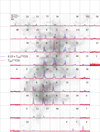 |
Fig. B.1 Spatial variation in 12CO and 13CO emission (blue and red respectively). The background is the 12CO integrated intensity. Each square shows the mean spectra within each grid position. The W(12CO)/W(13CO) line ratio for > 3σrms emission is shown in black. Note that Tmb(12CO) has been multiplied by 0.33. Large line ratios > 50 are seen when 12CO is detected but almost no 13CO. |
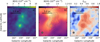 |
Fig. C.1 Estimate of molecular gas fraction in MBM12. Panel a shows total hydrogen column density from NICEST extinction maps. Panel b shows the atomic hydrogen column density from HI4PI Collaboration (2016). Contours of N(H) = [3,4,5,6,7,8] × 1021 cm−2 are shown in green. Panel c shows the molecular gas fraction from the combination of these observations with contours of fmol = [0.5,0.6,0.7,0.8]. |
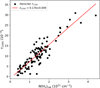 |
Fig. D.1 Dust opacity estimate at 1200 GHz for MBM12 using the column densities N(H2)cal of Remy et al. (2017) as a calibrator in the case of a molecular gas fraction fmol of 1. The resulting dust opacity is shown. |
The value of XPLMax is the maximum of the PL Range column of Table E.1, just before the excess peak (Fig. 7). Figures E.1 a and e show the three masks for the two isotopologues. We also plotted the histograms of N(H2), N(CO) and [CO/H2] for these regions (panels b−d and f−h for 12CO and 13CO respectively). Regarding the maps we note that the EX mask is always at the edge of the cloud. For 13CO it follows the order of EX → PL → LN from outside to inside the cloud. However, for 12CO, there is a filamentary structure on the inside that is PL, which is not seen in 13CO. This is likely related to 12CO transitioning to high optical depths, while 13CO is still optically thin. The N(CO) PDFs are very different between masks. The LN mask in both isotopologue has a broad lognormal distribution centred around 1017 cm−2, while the PL mask is bimodal for 12CO and single peaked for 13CO. The EX mask has the lowest peak value for both isotopologues. The abundance PDFs show mostly lognormal distributions, with a possible powerlaw at the low abundance end for 12CO, while for 13CO the three distributions are lognormal, with the peak abundance decreasing in the order LN → PL → EX. We consider these masks to segment the MBM12 map into distinct physical regions based on CO chemistry and optical depth effects. The detailed reasons why X(CO) change in these statistical behaviour requires additional investigation over multiple clouds and other spectral lines. Comparison with radiative transfer and chemistry simulations will also be helpful.
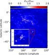 |
Fig. D.2 Dust opacity per nucleon, σν from multi-wavelength modelling for anti-centre fields from Remy et al. (2017) as a ratio of the commonly used dust opacity from Hildebrand (1983), with β = 2. The insert is a zoom-in of MBM12, with the same colour scale. |
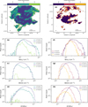 |
Fig. E.1 Single-isotopologue segmentation of MBM12 based on X(CO) PDF decomposition. Top panels: Spatial distribution of lognormal (LN, left) and power-law (PL, right) classified regions for 12CO (panels a-d) and 13CO (panels e-h), overlaid on the N(H2) map. The excess (EX) regions appear predominantly at cloud edges. Lower panels: Histograms of N(H2), N(CO), and [CO/H2] for pixels in each classification |
Appendix F Considerations when interpreting αvir
Most forms of the observational αvir for MCs are the ratio of internal kinetic energy to gravitational energy (e.g. Bertoldi & McKee 1992). There has been an ever-evolving discussion on the (ir)relevance of virial parameters. One’s interpretation of αvir varies based on whether one assumes static or dynamic MCs. Forty years ago, it was common to conclude that MCs are in virial equilibrium from the Larson σv ∝ R0.5 scaling relation, and to use that to calculate the cloud virial mass (Solomon et al. 1987; Mooney & Solomon 1988; Lis & Goldsmith 1989). From similar static assumptions, some have interpreted αvir < 1 as a sign of other supporting forces such as internal turbulence or magnetic fields (Bertoldi & McKee 1992; Kauffmann et al. 2013). Those discussed above used an assumption of virial equilibrium to either calculate masses or infer some unmeasured force. For the dynamic assumption of MCs, the value of αvir can be used as a measure of (un)boundedness of a cloud. There the assumption is that internal kinetic and gravitational energies are the only relevant energies, and so αvir > 1 − 2 can be used as a simple binary measure for gravitational boundedness. Many users of this approach do flag its tentative nature (Rosolowsky et al. 2008; Friesen et al. 2016; Friesen & Jarvis 2024; Oakes et al. 2025). Strictly speaking, this approach in particular has no way to distinguish if the cloud is gravitationally collapsing (no supporting forces), in pressure equilibrium (unobserved supporting forces), dispersing (unobserved forces stronger than gravity) or fragmenting (Chieze 1987). Virial parameters are a local measure and ignore external pressure, large-scale velocity gradients, and rotation (Ballesteros-Paredes 2006; Chevance et al. 2023). There are also observational biasing effects, such as background subtraction, sampling due to line excitation and variable emission-to-mass conversion factors that may lead to artificially small αvir (Singh et al. 2021). Some have therefore proposed alternative observational estimators of gravitational stability (Li et al. 2015; Krumholz et al. 2025). The observational virial parameter from PPV cubes is different from a 3D virial parameter in a simulation due to projection. In simulations, one can directly calculate gravitational, kinetic and magnetic energies. Some simulations of MCs suggest that observational virial parameters are not associated with cloud stability at all, due to tidal and projection effects (Dib et al. 2007; Kim et al. 2021; Offner et al. 2022; Lee et al. 2025). These considerations show that one should be upfront about assumptions when doing virial analysis, and that the conclusions from a virial analysis alone are only tentative without combination with independent measures.
All Tables
All Figures
|
Fig. 1 Left: position of MBM12 relative to the galactic disk. The colour scale shows the Planck 857 GHz dust continuum, and the contours are the neutral hydrogen column density with contours at levels [1.0, 1.2, 1.4] ×1021 cm−2 from the HI4PI all sky survey (HI4PI Collaboration 2016). The beam sizes of Planck 857 GHz (orange) and H14PI (white) are shown in the bottom left. Assuming a distance of 252 pc to MBM12 and a solar height of 20 pc above the galactic plane, the distance of MBM12 from the galactic plane is shown in white. Right: zoom-in of MBM12 with the positions of T Tauri stars from Meeus et al. (2009) shown with cyan [×] markers. The observing field of view of the TRAO and Herschel observations used in this work are shown in white and yellow, respectively. A distance scale is shown in the bottom right. |
| In the text | |
|
Fig. 2 Spatial variation in the 250 μm dust opacity in MBM12, κ1200, derived from the ratio of τ1200 and AK, accounting for the variable molecular gas fraction. The conversion assumes an extinction curve with RV = 3.1, and N(H)/Ak = 1.67 × 1022 cm−2 mag−1 (Cardelli et al. 1989; Bohlin et al. 1978; Lewis et al. 2022). Contours of κ1200 = [0.16,0.18,0.2,0.22,0.24] cm2 g−1 are overplotted. |
| In the text | |
|
Fig. 3 Mean spectra over the entire MBM12 field. The velocities of each peak are indicated. |
| In the text | |
|
Fig. 4 Integrated intensity (a and d), intensity weighted mean velocity (b and e), and intensity weighted velocity dispersion (c and f) for 12CO (top) and 13CO (bottom) for MBM12 as observed with TRAO. The sub-regions of MBM12 referenced in the text are labelled in red. |
| In the text | |
|
Fig. 5 Comparison of H2 and CO quantities observed in MBM12 with Herschel and TRAO. We compare N(H2) with CO linewidths W(CO), X-factors X(CO), 12CO excitation temperature Tex, CO column density N(CO)lte, and CO abundances [CO/H2]lte. Panels a)-c) and d)-l) have different colour scales. Panels d)-f) have linear fits shown in black lines, with the slope annotated on the respective panel. The linear striations at low N(H2) in panels j) and k) are artefacts of the sigma clipping in the W(CO) estimates. |
| In the text | |
|
Fig. 6 Top: opacity-calibrated N(H2) map from Herschel observations. Bottom: dust-opacity-calibrated N(H2) PDF with Herschel for MBM12. The Herschel map covers only the southern half of MBM12. |
| In the text | |
|
Fig. 7 Ratio of N(H2) and CO line area for 12CO and 13CO ground state rotational transitions in the southern half of MBM12. The figures are in units of XGal = 2 × 1020 cm−2 (K km s−1)−1. The beam size and linear scale are shown at the bottom left and right respectively. Contours of N(H2) are shown in red at levels of [1, 2, 5, 8, 10] × 1021 cm−2. The bottom panel shows the PDFs of X(12CO) and X(13CO). |
| In the text | |
|
Fig. 8 Carbon monoxide column density N(CO) for MBM12, derived from TRAO 12CO and 13CO (J = 1-0) observations. The map shown on the top was estimated with standard LTE assumptions to derive N(13CO) and converted to total N(CO) with the isotopologue ratio function from Szűcs et al. (2014). The bottom panel shows the PDF for the N(CO) map. |
| In the text | |
|
Fig. 9 Map of CO abundance relative to H2 column densities in the southern part of MBM12. The top panel shows N(CO) estimated from LTE assumptions. The bottom panel shows the abundance PDF. |
| In the text | |
|
Fig. 10 Hierarchical structure and virial estimates for MBM12 with 13CO (J = 1-0) observations with the TRAO. Panel a: centre velocities for dendrogram structures. The plot was made by plotting the largest-scale structures first with a single colour corresponding to their Vcen, and then the smaller-scale structures have been plotted on top. Panel b: virial parameter estimates for dendrogram structures. The plot was made in the same way as panel a, but with the colour defined by the value of αvir. Panel c: tree diagram for 13CO observations of MBM12. The tree diagram is coloured according to the value of Vcen for the structure with the same colour scale as panel a. The structures with the four largest-scales are shown in red. Panel d: tree diagram for αvir estimated with the 13CO observations of MBM12. The tree diagram is coloured according to αvir with the same colour scale as panel b. |
| In the text | |
|
Fig. 11 Scale dependence of 13CO dendrogram structures in MBM12. The colours are for the Horseshoe (blue), North Compact (green), eastern Bow (yellow), western Bow (purple), southern North Diffuse (black), and eastern North Diffuse (grey). Broken power law fits are also shown, with the respective fit values in Table 1. Vertical lines indicate the power law breaking point. The vertical axis in panels a-c (Mst/R2st) is in units of solar mass per square parsec. |
| In the text | |
|
Fig. 12 Top left: MBM12 H2 column density map. Top middle: Network of filaments reconstructed with FilDReaMS, with the largest bar width, Wb, per pixel shown. Top right: same network of filaments with the smallest Wb per pixel shown. Middle left, middle, and right: Map of the relative orientation for the smallest Wb filaments, most significant filaments across Wb, and largest Wb filaments, respectively. BPoS orientation is visualised using line integral convolution in grayscale in the background. Bottom left, medium, and right: histograms of relative orientations as a function of N(H2) for the smallest Wb filaments, most significant filaments across Wb, and largest Wb filaments respectively. |
| In the text | |
|
Fig. B.1 Spatial variation in 12CO and 13CO emission (blue and red respectively). The background is the 12CO integrated intensity. Each square shows the mean spectra within each grid position. The W(12CO)/W(13CO) line ratio for > 3σrms emission is shown in black. Note that Tmb(12CO) has been multiplied by 0.33. Large line ratios > 50 are seen when 12CO is detected but almost no 13CO. |
| In the text | |
|
Fig. C.1 Estimate of molecular gas fraction in MBM12. Panel a shows total hydrogen column density from NICEST extinction maps. Panel b shows the atomic hydrogen column density from HI4PI Collaboration (2016). Contours of N(H) = [3,4,5,6,7,8] × 1021 cm−2 are shown in green. Panel c shows the molecular gas fraction from the combination of these observations with contours of fmol = [0.5,0.6,0.7,0.8]. |
| In the text | |
|
Fig. D.1 Dust opacity estimate at 1200 GHz for MBM12 using the column densities N(H2)cal of Remy et al. (2017) as a calibrator in the case of a molecular gas fraction fmol of 1. The resulting dust opacity is shown. |
| In the text | |
|
Fig. D.2 Dust opacity per nucleon, σν from multi-wavelength modelling for anti-centre fields from Remy et al. (2017) as a ratio of the commonly used dust opacity from Hildebrand (1983), with β = 2. The insert is a zoom-in of MBM12, with the same colour scale. |
| In the text | |
|
Fig. E.1 Single-isotopologue segmentation of MBM12 based on X(CO) PDF decomposition. Top panels: Spatial distribution of lognormal (LN, left) and power-law (PL, right) classified regions for 12CO (panels a-d) and 13CO (panels e-h), overlaid on the N(H2) map. The excess (EX) regions appear predominantly at cloud edges. Lower panels: Histograms of N(H2), N(CO), and [CO/H2] for pixels in each classification |
| In the text | |
Current usage metrics show cumulative count of Article Views (full-text article views including HTML views, PDF and ePub downloads, according to the available data) and Abstracts Views on Vision4Press platform.
Data correspond to usage on the plateform after 2015. The current usage metrics is available 48-96 hours after online publication and is updated daily on week days.
Initial download of the metrics may take a while.